The Stock Market Crash and Banking Panic

Following the American Civil War, railroad construction grew dramatically.Footnote ¹⁰ The scale of railroad operations, with large fixed costs before any revenue could be obtained, meant that firms had to obtain external financing in significant quantities. Some large roads were able to issue equity, but the majority relied on loans and bonds. For example, a December 1872 Commercial and Financial Chronicle (CFC) provides information on the capital structure of 408 railroads, of which only 159 had issued equity; fewer than two dozen equities were actively traded on the New York Stock Exchange. Much of the debt of smaller firms was often placed with foreign investors, and it did not trade actively. Investors in those issues did not always see actively quoted prices for their bonds, and they may have been updated on the firm's status when (if) they received a scheduled interest payment.

Jay Cooke & Co. was one of the most important and well-known institutions and had marketed $500 million of bonds issued by the Union during the Civil War. After the war, the firm continued to handle a majority of government refunding operations. The firm also financed the construction of the Northern Pacific Railroad, which was beset with major financial difficulties. Cooke's resources diminished in 1873 as a U.S. Treasury bond issue, of which Cooke was responsible for half, sold slowly in Europe; marketing of Northern Pacific bonds was similarly difficult.

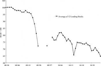
On 8 September the New York Warehouse & Security Company suspended operations because of insolvency. The company had loaned money for construction of the Missouri, Kansas, and Texas which could not be repaid. Five days later, Kenyon, Cox, & Co., of which Daniel Drew was a general partner, suspended because it could not collect on a $1.5 million railroad loan to the Canada Southern. Over the course of the week, some small financial institutions failed, and the New York and Oswego Midland Railroad failed to meet $1 million of its obligations on the seventeenth and suspended operations. On 18 September two smaller firms declared insolvency, but the major event was the closing of the venerable Jay Cooke & Co. Failure of the Northern Pacific led to the failure of its major creditor, Cooke. An index of leading stocks fell 4.8 percent that day, after falling 3 percent the day before; it had also fallen the three days prior to that. Figure 1 shows the daily closing level of the index over the September—October 1873 period.Footnote ¹¹

Figure 1

DAILY AVERAGE OF 12 LEADING STOCKS, AUGUST—OCTOBER 1873

Notes: The index is a price-weighted average of 12 regularly quoted stocks (Chicago & Northwestern, Erie, Harlem, Lake Shore, New York Central & Hudson, Ohio & Mississippi, Pacific Mail, Rock Island, St. Paul, Union Pacific, Wabash, and Western Union). Prices are last transactions each trading day, taken from various issues of the New York Times. Prices for 26 September, during the exchange closure, are midpoints of curb market prices as reported in the Commercial and Financial Chronicle.

The decline intensified the next day. Fisk & Hatch, another major firm, suspended operations, again due to calls on railroad creditors who could not pay. Runs on the Union Trust Company and Fourth National Bank were reported, as banks began refusing to certify checks from suspect banks. The secretary of the Union Trust Company vanished with $250,000 of the firm's money, increasing uncertainty. Other firms suspended payments: the New York Times lists 23 brokers who suspended on the eighteenth and nineteenth. Rumors of insolvency flew, both for names that were eventually found to be insolvent as well as solvent ones. The stock index declined 7.9 percent. Saturday morning, 20 September, was even worse. Volume was heavy on the exchange and stocks declined precipitously. The Governing Committee closed the exchange after an hour's trading, until further notice. The market had declined 11.2 percent since the previous close. Banks in New York and elsewhere suspended payments of currency.

The New York Clearing House authorized $10 million in clearinghouse certificates to settle interbank balances. While the Stock Exchange was closed, well-known banking houses continued to suspend operations as their situations became clear. The Treasury provided liquidity by purchasing $24 million in bonds and the Clearing House issued another $10 million in certificates. Ultimately, the Treasury would inject a total of $26 million into the system and approximately $25 million in clearinghouse certificates would be issued. The Stock Exchange reopened on 30 September. The banking panic peaked on 4 October, when New York City bank reserves stood at 12.8 percent. By the end of October, immediate effects of the crisis were over, and banks had resumed conversion of deposits into currency.

The Market for Privileges

An active, over-the-counter option market existed during the latter part of the nineteenth century. The structure of the market was well-defined. Wealthy individuals such as Russell Sage sold blocks of puts and calls to brokers who resold them to small speculators. This arrangement reduced counterparty credit risk, because small speculators with unknown credit were allowed only to purchase options and were required to pay for them in advance. The options were known as “privileges” because the purchaser of a call, for example, had the privilege of calling for the stock at the strike price, or not calling for it, at his option.Footnote ¹²

All options were American style and could be exercised at any time prior to expiration. There was no organized trade of previously issued options. Contemporary accounts report that options were sometimes traded after issuance, but the discussions are usually associated with potential defaults of option issuers. When an issuer could not be found to take or deliver stock, and it was suspected that he would default, the options were traded among speculators at a discount to the market value of an otherwise identical option without default risk.Footnote ¹³

On modern option exchanges, an option contract is specified with a given strike price and the option price is negotiated between buyer and seller. In 19th century option markets, this convention was reversed. Option contracts were sold for a fixed price, but the strike price was negotiated between buyer and seller. A call might be quoted as “1 1/8,” for example, meaning that the strike price for the option was $1 1/8 above the market price for the underlying. Similarly, a put quoted at “1 1/8” was understood to be struck at $1 1/8 below the market price of the underlying.

The standard option contract was for 100 shares of the underlying stock, expiring one month after issuance. The price was fixed at $106.25, or $1 per share plus commission. Some brokers advertised contracts for fewer shares at a proportional premium (for example, an option on 50 shares for $50 plus a proportional commission) or for a different term, but one month options on a round lot of stock appear to have been the focus. For example, broker indications in the 25 January 1873 CFC have the following description: “Lapsley & Bazley, Brokers, 47 Exchange place, quote stock “privileges” (signed by responsible parties), 1 per cent premium for 30 days, and 1 1/2@2 per cent premium for 60 days at prices varying from the market as follows: …”. In the same issue, an advertisement for the broker elaborates by stating “$100 and commission will purchase a first class contract, giving you the privilege of calling for or delivering (i.e., being ‘long’ or ‘short,’) 100 shares of any active stock, at any time in 30 or 60 days.”

When option quotes began appearing in the CFC in January 1873, one month options cost $100 plus commission. By mid-February 1873, Lapsley & Bazley's quotes had changed from stating “1 per cent premium” to “1@1 1/4 per cent premium.” Nonetheless, Lapsley & Bazley's text ads from mid-1873 continue to refer to $100 option prices. By January 1874, one month contracts clearly appear to have become standardized at $100 plus commission. Consistent with a nonstandardized environment for option sales in 1873, the quote ranges and price ranges may have provided some flexibility for brokers to tailor contracts to market conditions or customer requirements. For the purposes of this article, I treat all of the one month quotes as reflecting a $106.25 all-in price of an option over the entire sample period.Footnote ¹⁴

The language of the contracts was simple, as shown in this 1870s market manual example of a put:

The example highlights treatment of dividends: any dividends paid during the life of the option went to the ultimate holder of the stock. This reduced the effective strike price of the options by the amount of the dividend. Robert Merton has noted that this method of dividend protection does not exactly offset the effect of the dividend, but the resultant “mispricing” is quite small.Footnote ¹⁶

Raw Data and Implied Volatility Calculations

Indicative option quotes were published in the Commercial and Financial Chronicle most weeks from January 1873 until June 1875. Brokers provided indicative ranges at which individuals could purchase puts and calls for roughly a dozen stocks. The universe of stocks was not constant, but it generally covered the actively quoted stocks. Quotes were for the distance from the spot price at which a call or a put would be struck. Although ads for the put and call brokers continued intermittently after this period, no other systematic reporting of indicative prices appears available.

Given the contract terms, option price, stock price, and relevant interest rate, I compute a Black-Scholes implied volatility and option delta for each one-month option in the sample. I take the midpoint of the indicative strike price range as the strike price. In recent research, Kairys and Valerio interpret these quote ranges (e.g., puts quoted as 3/4@1) as bid and ask quotes. I deviate from this practice for two reasons. First, my reading of advertisements and brokerage literature suggests that the retail customers targeted in these ads would never have been offered the opportunity to write options and hence would never have seen bid quotes for options.Footnote ¹⁷

Second, while the “@” symbol is sometimes used to separate bid and ask quotes, writers during this period also used the symbol to denote approximate ranges. The following two quotes describing market conditions provide evidence for this assertion: “Money continues very easy on call loans, and the rates have ranged from 3@5 per cent….” and “The stock market has been without decided movement of importance until to-day, when a bear movement set in, led by Wabash, … which sold down to 25, and carried down the balance of the list to the extent of 1/2@2 per cent.”Footnote ¹⁸ Based on these reasons, I interpret the notation as a range of ask quotes rather than bids and asks.

Interest rates for prime commercial paper, also collected weekly from the CFC, are used as the riskless discount rates.Footnote ¹⁹ The stock price is taken as the midpoint of the daily high and low on Friday, the trading day immediately prior to publication of the paper. If the stock did not trade, the CFC reported bid and ask quotes, and I use those values. To account for the possibility of early exercise, I use a 100 step binomial tree to compute the implied volatilities and deltas. Use of the Black-Scholes model does not mean that it is assumed to be the correct valuation model, but it is used to convert option prices into a well-understood common metric.

I identify 17 stocks in the sample that generally had option quotes in the broker ads. Many of these stocks had option quotes throughout the sample, but some did not. For example, options on Chicago & Northwestern preferred stock were quoted regularly prior to the crisis, but not at all after. Options were quoted regularly on Northwestern common stock after the crisis, but not before. (Both types of equity were traded pre- and postcrisis.) Also, Boston, Hartford & Erie options were quoted regularly prior to the crisis, but not after. This stock had fallen 75 percent to $2 per share by this time. The stock was in receivership since 1872 and was being reorganized.

To facilitate comparison of the data over time, I standardize the implied volatilities for each stock to represent hypothetical 25 delta puts, 25 delta calls, and 50 delta options. Delta is the first derivative of the call price function with respect to the price of the underlying asset, and it is approximately the probability that an option will expire in-the-money. Therefore, a 25 delta put has approximately a 25 percent chance of expiring in-the-money, as does a 25 delta call. In modern OTC markets, option trades are often specified in terms of delta. So-called risk reversals are common trades including the purchase of a 25 delta call and the sale of a 25 delta put. The resulting trade is supposed to be delta-neutral: at initiation, the delta of the put offsets the delta of the call and the position value has no dependence on the value of the underlying asset.

I compute the deltas for the put and the call and assume a linear relation between deltas and implied volatilities. In other words, I assume a linear volatility skew in delta.Footnote ²⁰ I convert put deltas into call deltas and linearly interpolate to find the 25, 50, and 75 delta call volatilities. The required 25 delta put volatility equals the 75 delta call volatility. For ease of presentation, I interchangeably use the terms “at-the-money (ATM)” and 50 delta for the remainder of the article. Because puts are valuable if the underlying asset declines in price, while calls are valuable if the underlying asset rises in price, the relative valuation of the two types of options translates directly into an implicit distribution of the asset price at expiration.

If quotes are available for only the put or call, but not both, I exclude that date from the sample. For the Boston, Hartford & Erie Railroad (a low-priced, high volatility stock), the interpolated data points are sometimes negative. Of the 29 dates with put and call quotes on this stock, I eliminate data on six dates for which an interpolated volatility is less than zero.

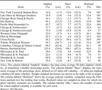
Table 1 displays the average at-the-money implied volatility and the average implied volatility skew for each stock. Also shown are the standard deviations of these series. For comparison, the table also shows the average realized volatility for each stock, computed with the Parkinson measure.Footnote ²¹ The ordering of stocks in the table reflects the typical ordering of the stocks in the newspaper.

Table 1

DESCRIPTIVE STATISTICS OF IMPLIED VOLATILITY BY STOCK

Notes:

The column labeled “Implied” displays the time-series average 50 delta implied volatility, in annualized volatility percentage points. The column labeled “Skew” displays the time-series average of the percentage skew, defined as (25 delta call volatility — 25 delta put implied volatility)/50 delta volatility. Sample standard deviations are shown to the right of the averages. The column labeled “Realized” shows the average realized volatility, computed using the Parkinson method over the trailing four weeks. Realized values are sampled on dates for which implied volatility estimates are available. The column labeled “Obs.” shows the number of dates for which implied volatility is available for each stock.

Sources:

See the text.

Aggregation and Implied Distribution Calculations

To aggregate the information from the entire set of stocks, I compute trimmed cross-sectional averages for each week in the sample. For the index of at-the-money implied volatility, the 50 delta volatility for each stock is averaged, excluding the highest and lowest values each week. The index of skew is computed as a “percentage volatility skew.” For each stock, I compute the 25 delta call volatility minus the 25 delta put volatility and then divide this value by the 50 delta volatility. Negative values mean that out-of-the money put volatility is higher than out-of-the-money call volatility, corresponding to a negatively skewed implied distribution for log returns. Percentage skews are then averaged across stocks, with the highest and lowest values trimmed.

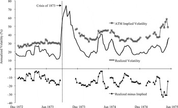
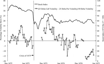
The implied volatility index is displayed in Figure 2, and the volatility skew index is displayed in Figure 3. Of the 105 weeks with option quotes in the sample, 95 of the trimmed averages represent 11 or 12 option volatilities. One week includes ten names, while the first five weeks of the sample represent seven or eight names. The smallest number of names represented is for a four week period in January and February 1875, when four names are included in the trimmed averages.

Figure 2

IMPLIED AND REALIZED VOLATILITY

Notes: The chart shows at-the-money (50-delta) implied volatility, realized volatility, and realized volatility minus implied volatility. Realized volatility is the trailing four week rolling standard deviation of stock returns, computed using the Parkinson range-based measure. Both series are equally-weighted averages of the individual stock volatilities. Averages exclude the highest and lowest component values each week.Sources: See the text.

Figure 3

PERCENTAGE VOLATILITY SKEW AND STOCK INDEX LEVEL

Notes: The stock index is a price-weighted index of 17 stocks for which option quotes are available. The volatility skew is an equally-weighted average, excluding the highest and lowest values each week, of individual implied volatility skews. Skew for each stock is computed as (25 delta call volatility — 25 delta put volatility)/50 delta volatility. A negative value indicates a negatively skewed implied distribution; a positive value indicates a positively skewed distribution.Sources: See the text.

Figure 3 also shows a price-weighted index of the 17 stocks in the option sample. The value for each stock is the midpoint of Friday's high-low range. If the high-low range is not available, but a single value is reported, I use that value. If Friday data are not available, I use the most recent available date. Note that this index is broader than the 12 stock index used in Figure 1, which focused on daily data. The index presented over the longer period includes some less active stocks, many of which did not trade every day.

Using the indexes of implied volatility levels and skews, I construct the implied distribution function for returns on a hypothetical, “typical” stock. Douglas Breeden and Robert Litzenberger have shown that the probability density function for the value of an asset at the expiration of a call option on that asset, f(S_T), is related to the call pricing function C(·) by the relation

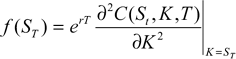
In this equation, S_t is the value of the asset at time t, K is the strike price of the option, r is the riskless discount rate, and the option expires at time T.Footnote ²² To compute f(S_T), I numerically differentiate the call pricing function for each date in the sample. Differentiation requires a continuous call pricing function, which is computed using a smoothed implied volatility method, similar to that used by Robert Bliss and Nikolaos Panigirtzoglu.Footnote ²³ I convert deltas into strikes on a 300 point grid and evaluate the Black-Scholes call pricing function using the linearly interpolated implied volatility. A logistic transform was employed to ensure sufficient gridpoints in the tails of the distribution for reliable computations. Given the numerical representation of the distribution, I convert the distribution over stock price to a distribution over log price returns, relative to the forward price. With this representation in hand, it is straightforward to integrate the function to compute desired statistics. The transformation to a return distribution facilitates interpretation of the skewness coefficient, in particular. The log return distribution is normal and symmetric under the benchmark lognormal distribution for prices, but the implied distribution can deviate from this in readily interpretable fashion.

Implied Volatility and Realized Volatility

Rational pricing of options implies cross-sectional consistency of option prices with the volatility of the underlying stocks. High volatility stocks should have higher option prices than low volatility stocks, if option prices rationally reflect the fundamentals (realized volatility). If pricing in the market for privileges simply reflects the whims of speculators looking for action, there is less reason to expect the relation. In this section, I test whether the cross-section of at-the-money implied volatility is, on average, consistent with the cross-section of realized volatility and find that it is.

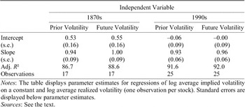
I first compute at-the-money implied volatility for each date and stock that it is feasible. On those dates, I also compute the realized volatility over the trailing four weeks using the Parkinson estimator. The statistical specification is to regress the log of the average implied volatility for a stock on the log of the average realized (trailing) volatility for that stock. The results are displayed in the first data column of Table 2 and appear highly consistent with a market that evaluated the relative risks of stocks appropriately. While the intercept is significantly larger than zero, indicating that implied volatility consistently exceeded realized volatility, the slope coefficient is significantly above zero and insignificantly different than unity.

Table 2

IMPLIED AND REALIZED VOLATILITY (dependent variable: log average at-the-money implied volatility)

Notes:

The table displays parameter estimates for regressions of log average implied volatility on a constant and log average realized volatility (one observation per stock). Standard errors are displayed below parameter estimates.

Sources:

See the text.

In the column labeled “Future Volatility,” results are displayed for the regression specification featuring the log of the average future realized volatility for each stock. In this case, parameter estimates are similar to the ones described above, although the slope coefficient is slightly closer to unity than before. The higher value is consistent with the idea that implied volatility is set in the market on a forward-looking basis and that extreme values of realized volatility are not always reflected one-for-one in implied volatility. If traders expect volatility to decline from an extremely high level after a shock, for example, they might not increase implied volatility as much as realized volatility had increased.

For comparison, the last two columns in Table 2 display regression estimates constructed using summary statistics for 25 short-term equity options over the 1991–1995 period.Footnote ²⁴ Slope estimates for the 1990s data are similar to the estimates for the 1870s. The slope coefficient is slightly smaller if trailing volatility is used in the regression, as compared to future volatility, but in both regressions the slope is insignificantly different from unity. The intercept is lower in the regression using the modern sample, reflecting the smaller gap between implied and realized volatility. I conclude that option traders in the 1870s appear to have assessed the appropriate implied volatility across stocks similarly to how option traders in the 1990s did.

Despite the strong relation in the cross-section, one could focus on the intercepts in the regressions, or the gap between implied and realized volatility, and conclude that option markets did a poor job assessing risk. The median implied volatility across stocks in the 1870s sample is 39 percent, while the median implied volatility gap (implied minus trailing realized volatility) is 14 percent. Roughly speaking, 14/39 or approximately 37/100 of the observed implied volatility was due to bias. In the modern sample, the median implied volatility across stocks is 22.9 percent, while the median implied volatility gap is 1.6 percent. Therefore, 1.6/22.9 or approximately 7/100 of the observed implied volatility was due to bias. To be convincing, a rational pricing explanation must simultaneously explain the large gap in the 1870s data and also the much smaller gap in the 1990s data.

Recent research has concluded that supply and demand pressures have a marginal effect on implied volatility beyond the impact of expected realized volatility. Nicolae Gârleanu, Lasse Heje Pedersen, and Allen Poteshman and, independently, Nicholas Bollen and Robert Whaley concluded that implied volatility is subject to buying and selling pressure (order flow).Footnote ²⁵ For example, Gârleanu et al. examined the 1996–2001 period and concluded that end users were net buyers of index options, which featured implied volatility higher than forecast realized volatility, and that end users were net sellers of single stock options, which featured implied volatility lower than realized volatility in their sample. This interpretation can readily be applied to explain the implied volatility gap during the 1870s, when a limited number of large agents sold options to small speculators who were allowed only to purchase options. I conclude that the persistent one-sidedness of the nineteenth-century equity option market explains the large gap between implied and realized volatility, but the one-way nature of trading did not eliminate the tight cross-sectional correspondence of implied and realized volatility beyond making all options somewhat “expensive.”Footnote ²⁶

Implied Volatility and Corporate Bond Spreads

I next evaluate the pricing of equity options by comparing the evolution of risks priced in the option market with the evolution of risks priced in the railroad bond market. Based on the original insights of Fischer Black, Myron Scholes, and Robert Merton, it is well known that corporate bond holders can be thought of as riskless bond holders who have sold puts to equity holders of the company.Footnote ²⁷ At maturity, bondholders receive at most the face value of the debt. If the value of the firm falls below the amount the firm owes, bondholders are entitled to the value of the company. Equivalently, holders of corporate bonds can be viewed as holding a portfolio that is long a similar riskless bond and short a put option on the firm, struck at the face value of the debt. Factors that change the value of the put therefore change the value of the risky bond's credit spread.

It is possible to test whether the pricing of the explicitly observed equity options is consistent with the pricing of the implicit options associated with credit spreads. If it is, I infer that the markets were integrated and that the participants in the two markets were pricing firm risks in similar ways. If option and bond prices reflect the same fundamentals, this is further evidence that markets were well aware of these fundamentals when pricing other assets, namely stocks.

I follow Frederick Mishkin in constructing an index of credit spreads using the yields on railroad bonds collected by Frederick Macaulay.Footnote ²⁸ For each month in the sample, the average yield of the five bonds in the lowest quarter of bond yields is subtracted from the average yield of the five bonds in the highest quarter. The bonds are all high grade, so the spread does not truly represent the difference between funding rates for high- versus low-quality issuers. Nonetheless, Mishkin concludes that the spread constructed in this fashion generally performs well.

I view the credit spread index as a put option and evaluate the sign and significance of factors that should impact the value of that option. I discuss these determinants individually. Effectively, these factors represent the first three moments of the probability distribution function of firm value.

First, Leverage. The strike price of the put is the debt level of the firm, and hence firm leverage is the ratio of strike price (face value of debt) to the price of the underlying (firm value). This is the inverse of the moneyness of an option, which is often defined as the ratio of spot price to strike price. If firm value declines relative to the face value of debt, then leverage increases and default is more likely, the value of the implicit put increases, and the credit spread increases. Leverage is computed as book value of firm debt and preferred shares divided by total firm value (book value of debt and preferred equity plus market value of common equity), averaged across all of the stocks in the option sample. Equity values are computed monthly, while debt values are linearly interpolated using approximately quarterly data as available from the CFC.Footnote ²⁹

Second, Volatility. Increased volatility of the firm value increases the likelihood of default, and hence the credit spread. I use the standard deviation of log stock returns, computed from the implied distribution of the “typical stock” at the end of the month, as a proxy for the typical firm volatility.

Third, Skewness. Increased skewness of the probability distribution of firm value decreases the likelihood of default, and hence the credit spread. As with the volatility, I compute the skewness from the implied distribution of the “typical stock” at the end of the month as a proxy for the skewness of the firm value distribution function.

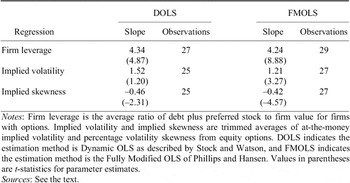
In summary, the Merton model predicts that the credit spread is positively related to leverage, positively related to equity volatility, and negatively related to skewness of the equity distribution. Table 3 displays regression results relating the credit spread index to each of the three variables. To guard against spurious inference in a short data set featuring a trend and possible nonstationarity, I employ two methodologies to estimate the relations. The left two columns of data present parameters from three regressions results based on James Stock's and Mark Watson's Dynamic OLS (DOLS) methodology, and the right two columns present results based on Peter Phillips's and Bruce Hansen's Fully Modified OLS (FMOLS) methodology.Footnote ³⁰

Table 3

INTEGRATION OF EQUITY AND BOND MARKETS (dependent variable: credit spread index between high and low grade railroad bonds)

Notes:

Firm leverage is the average ratio of debt plus preferred stock to firm value for firms with options. Implied volatility and implied skewness are trimmed averages of at-the-money implied volatility and percentage volatility skewness from equity options. DOLS indicates the estimation method is Dynamic OLS as described by Stock and Watson, and FMOLS indicates the estimation method is the Fully Modified OLS of Phillips and Hansen. Values in parentheses are t-statistics for parameter estimates.

Sources:

See the text.

There is evidence from both methods that an increase in firm leverage is associated with an increase in the credit spread, and that a decrease in skewness is associated with an increase in the credit spread. For equity volatility, the results are correctly signed for both techniques, and it is significant for the FMOLS results.

I conclude that the equity and option markets were reflecting the evolution of firm riskiness over time in ways that mirrored the conclusions of the corporate bond market. Credit spreads on railroad bonds moved in exactly the fashion predicted by modern theoretical models, relative to the information as perceived by the equity market. This effect appears in the sample despite the fact that the firms represented in the credit spread index are not the same firms as in the equity index. I interpret this as evidence in favor of integration of the bond and equity markets, as well as rationality of the option market's pricing.

Did the Option Market Expect a Crash?

Visual inspection of Figure 2 is a key first step in interpreting evidence on option market crash expectations. The figure displays the at-the-money implied volatility index and an equivalent index of trailing realized volatility, along with the difference between the two. Realized volatility is computed using the Parkinson measure over the previous four weeks of daily stock prices. At-the-money implied volatility is often used as a measure of the market consensus expected volatility over the life of the option.

The chart tells a simple story. Implied volatility always exceeded trailing realized volatility, but it roughly followed the rises and declines of realized volatility. When the market was in flux, implied volatilities increased, and when the market was quiet, option volatility tended to fall. An interesting exception to this pattern was the period prior to the 1873 crisis. From January to September, implied volatility trended upward from around 25 percent to around 30 percent, even as realized volatility declined. The gap between implied and realized volatility, which averaged around 10 percentage points over the first half of the year, settled around 15 percentage points immediately prior to the stock market crash. This value corresponds roughly to the gap between implied and realized volatility over the remainder of the sample, after the crash. Even if one discounts the entire average gap between implied and realized volatility, the gap widened prior to the crash, which is consistent with an increased perceived likelihood of substantial stock price movements.

Figure 3 displays the percentage volatility skew index over time. Negative values of this index indicate that 25 delta puts have a higher implied volatility than 25 delta calls, which can be interpreted as increased fears of downside risk (relative to the normal benchmark). Because option implied distributions reflect risk-neutralized distributions, incorporating risk and risk aversion, an increase in negative skewness could indicate either increased fears of a decline or an increase in the marginal utility of wealth in those states of the world. Similarly, increased positive skewness is often interpreted as reflecting increased likelihood of price increases in the underlying. The sign and magnitude of the implied volatility skew is often interpreted as a sentiment indicator of future movements in the underlying asset, and that is the approach taken here.

Skewness became quite positive in May 1873, providing quantitative insight into the May 1873 warnings by the Bankers' Magazine about margin loans and the “growing mania for gambling which is one of the worst features of the day.”Footnote ³¹ Skewness declined from this peak, as the market stayed roughly flat and implied volatility remained high. Immediately prior to the September crash, skewness turned negative, indicating negative sentiment and increased fears of a stock market decline. This drop occurred as the aggregate market fell slightly. It is worthwhile to note that the observations for option prices in September 1873 are for the sixth and the thirteenth, as first signs of the crisis were appearing, but before the free-fall and closure of the market. By February 1874 skewness increased again, moving upward at the same time as the stock market recovered from the crash. Skewness then declined again, apparently mirroring the market's movements to mid-1874. Finally, the option market appeared to be pricing in substantial negative skewness in the first half of 1875.

Observing the implied volatility and skewness over time is interesting and informative, but they can be difficult to reconcile. If implied volatility is increasing, but the implicit skewness is becoming more positive, is that interpreted as good or bad for equities? The level of implied volatility reflects the absolute price of equity risks, while the implicit skewness reflects the relative pricing of upside versus downside risk. The measures are not orthogonal, and the joint effects are difficult to gauge from time series charts of each. This points toward a more integrated approach.

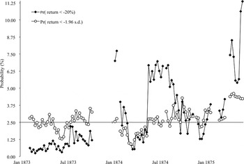
Figure 4 displays the risk neutral probability of a crash computed from option prices. At each point in time, I use the at-the-money implied volatility index and the volatility skewness index as volatility inputs to compute the risk neutral distribution of returns to a representative stock. I integrate this cumulative density function of terminal return to compute two probabilities. First, I compute the probability of a monthly log return lower than 20 percent below the forward rate (which is the mean of the risk neutral distribution of prices). Second, I compute the probability of a monthly log return less than 1.96 monthly standard deviations below the forward rate. The first measure gives a pure measure of downside risk. If this value changes, it can be because the volatility of the distribution changed, or because the skewness of the distribution changes. It intentionally aggregates the two into a number which is interpretable on its own; a similar computation was carried out by David Bates and Roger Craine in examining the probability of a tail event around the Crash of 1987.Footnote ³²

Figure 4

RISK NEUTRAL PROBABILITY OF CRASH

Notes: The estimated probability of the typical log stock return being lower than −20 percent at the end of the next month is displayed, along with the estimated probability of the return being lower than −1.96 standard deviations. Both return measures are constructed relative to the forward price, which is the mean under the risk-neutral distribution. The implied distribution for the typical stock is constructed using the at-the-money volatility and percentage volatility skew indexes constructed in the paper.Sources: See the text.

The second measure specifically focuses on skewness. It can be compared to the probability under a symmetric normal distribution, which is approximately 2.5 percent. Of course, these calculations should be taken as convenient representations of the general changes in option-implied probabilities, not as exact calculations. Looking across all stocks in the sample, the average strike price is approximately 5 percent out of the money, so extrapolating to a 20 percent change in stock prices is clearly asking quite a bit from the data.

Inspection of Figure 4 reveals a story of increasing perceived risks. As suggested earlier, the market appeared quite optimistic about stock prospects in May 1873, when the probability of a left tail event dipped dramatically, but these good feelings faded as the summer progressed. The likelihood of a lower than −20 percent return was very low during the first part of the year, but it increased over the year. There is no indication that the market factored in a substantial likelihood of a crash, but I nonetheless conclude that the market was concerned about the possibility of sharp moves to the downside and that this concern grew over the year. Investors appear to have been grown less optimistic as the year progressed. This conclusion is based on the implied distribution evidence presented in Figure 4 as well as the evidence shown in Figure 2 regarding implied and realized volatility.

When option quotes reappeared in January 1874, the market began assessing a substantial downward move as a low probability event. This corresponds to the recovery in the stock market level at this time. By mid-year, this optimism had faded as the market declined and volatility increased again. By early 1875 realized and implied volatility began trending upward, and the skewness became decidedly negative. The result was a sharp increase in the implied probability of a decline in the market. The highest probability of stock returns less than −20 percent occurred at the very end of the sample, which suggests a connection between this spike in downside risk and the stoppage of indicative quotes.

The option-implied probabilities of a crash during mid-1874, when postcrisis realized volatility peaked, are higher than during 1873. This does not invalidate the interpretation that some fear of a crash had crept into the market in 1873, but it highlights the fact that the crash fears that year, at the market-wide level, were not substantial. I do not claim that the market was a perfect forecaster, or that the crash probability peaked immediately prior to the crash. Rather, the more modest claim is that the option market perceived more risk in mid-to-late 1873 than it did in early 1873, even as the realized volatility of stocks declined. Equity, option, and bond investors generally agreed on the riskiness of the market, and they perceived the market as somewhat riskier in mid-to-late 1873 than at the start of the year.

The Domestic Environment

Matthew Simon reported that the economic environment for railroads deteriorated progressively during the early 1870s. He reported that one railroad had defaulted in each of the years 1868–1870, three defaulted in 1871, and 12 in 1872. During the first nine months of 1873, at least 35 roads defaulted. These 35 firms had bonds outstanding worth $92 million, which is comparable to $135 million outstanding for the 37 railroads defaulting prior to 1873.Footnote ³⁶ Railroads are high-fixed-cost ventures, and balance sheets were stretched thin during this period. Banks loaned money to railroads and acted to issue bonds afterwards. If the bonds could not be placed, the financial institutions retained the risk and their balance sheets deteriorated. As noted earlier, several high profile institutions failed in 1873 precisely because they were exposed to railroad debts that were not paid. This verifies the existence of Mishkin's two balance sheet factors that lead to financial crises. The fundamental economic environment led to increased leverage that caused banks to fail.

Mishkin's third factor relates to interest rate increases. Mishkin notes that the commercial paper rate increased in August 1873, verifying his prediction. Moving beyond Mishkin's analysis, it is also the case that there was deflation immediately prior to the crisis, raising the real interest rate paid by firms. From December 1872 to August 1873, the Warren and Pearson wholesale price index fell 2.9 percent; the index peaked in April 1873. This deflation may have been surprising, given the volatility of prices: the index averaged an annual decline of 8.6 percent from 1865 to 1870 but the annual inflation averaged 3.1 percent in 1871 and 1872.

Mishkin's fourth factor, the catalyst for financial crises, is the failure of high profile financial institutions. There is universal agreement that the crisis in the United States was sparked by failures of financial institutions such as Jay Cooke & Co. in September 1873.

Mishkin examined interest rates, credit spreads, and stock prices and found evidence generally supporting the asymmetric information explanation for the timing of U.S. financial crises in the nineteenth and early twentieth century. He finds little support for declining stock prices prior to the 1873 crisis. The stock index shown in Figure 3 displays a 10.4 percent decline from February 1873 to August 1873, evidence at a broad level for the predictions of his theory. In what follows, I examine prices from the equity, option, and credit markets and provide detailed evidence further supporting his propositions.

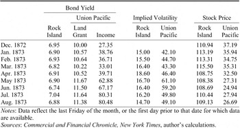
Table 4 presents evidence that money was not indiscriminately flowing into U.S. assets, bidding up prices. The results support the conclusion that any increased uncertainty in the nine months prior to the crisis was concentrated unevenly across firms. The first column shows yields for debt issued by the Chicago, Rock Island and Pacific Railroad, and the yield appears quite stable just below 7 percent. The next two columns show bond yields for Union Pacific, whose investors appear to have been less sanguine. The yield spread for Union Pacific Land Grant bonds over Rock Island bonds ended 1872 around 3 percentage points, but the spread grew to nearly 5 percentage points during the summer of 1873. The spread on Union Pacific income bonds ended 1872 around 20 percentage points and blew out to over 70 percentage points by the end of the summer.

Table 4

ASSET PRICES PRIOR TO THE CRISIS OF 1873

Notes:

Data reflect the last Friday of the month, or the first day prior to that date for which data are available.

Sources:

Commercial and Financial Chronicle, New York Times, author's calculations.

The next two columns in the table display the ATM implied volatility from Rock Island and Union Pacific stock, demonstrating that Rock Island volatility was somewhat steady around 16 percent, but that Union Pacific volatility started out higher and subsequently increased, peaking in early summer. The final two columns display prices for the two stocks, with Rock Island prices increasing a bit during the first three months of the year before dropping back to virtually the same level, whereas Union Pacific prices were declining much of the year as the firm was buffeted by the Credit Mobilier scandal. The data are representative in that several other firms in the sample had relatively stable stock prices and implied volatilities, while more speculative “fancies” such as Union Pacific, Pacific Mail, and Columbus, Chicago and Indiana Central displayed declining stock prices and increasing volatility. A coherent explanation of the crisis should incorporate this disparity of risks that the market was pricing across firms.

The previous illustration can be made more rigorous. I test whether the 12 railroad stocks in the index constructed previously in the article (excluding preferred stocks and the Boston, Hartford & Erie, which was in receivership) show a significant relation between leverage and stock returns. If investors were wary of levered stocks that were more dependent on the debt markets and more dependent on cash flow to pay debt, those stocks would have been penalized prior to the crisis. Alternatively, less levered stocks would have been rewarded with higher stock prices. This result is precisely the one found in the data. The five lowest leverage stocks (with a December 1872 debt / (debt + equity) ratio averaging 0.35) rose in price, on average, 3.3 percent from 27 December 1872 to 29 August 1873. The five highest leverage stocks (leverage of 0.81) fell 17.8 percent. A simple cross-sectional regression of stock price change over this period on December 1872 leverage yields a coefficient for leverage of −0.42 with a t-statistic of −4.38. The regression R ² is 66 percent.Footnote ³⁷ In the months prior to the crisis, equity investors penalized highly levered firms and rewarded firms with less leverage, indicating that they were wariest of highly levered, risky firms.

The prediction that credit spreads between high and low grade bonds should widen prior to a crisis, representing a relative increase in agency costs for lower quality borrowers, is not supported in Mishkin's data for the Crisis of 1873. The credit spread illustration presented above suggests that Mishkin's result is due to the coarseness of his data. As described earlier, he uses the spread between high- and low-yield railroad bonds collected by Macaulay, but these bonds represent high quality borrowers only. The finding that the yield spread between Union Pacific and Rock Island widened prior to the crisis suggests that an index constructed from a wider cross-section of bonds would resolve the anomaly.

The International Environment

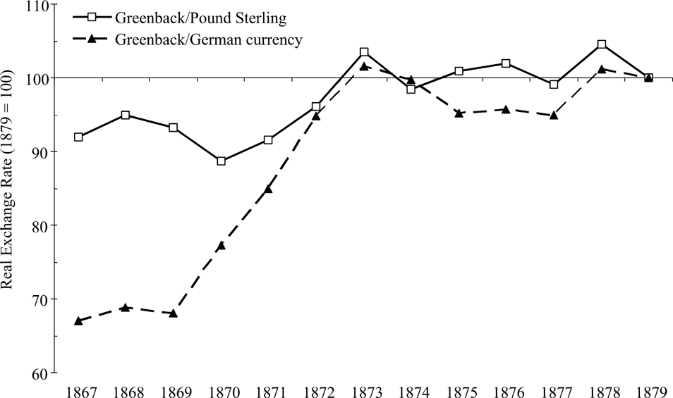
Figure 5 presents, for the years 1867–1879, estimated real exchange rates for the U.S. dollar versus the pound sterling and the German currency.Footnote ³⁸ The rates are indexed to 100 in 1879, when the United States effectively returned to a fixed exchange rate with Britain and other gold standard countries such as Germany.Footnote ³⁹ Based on the figure, I conclude that the floating greenback did not insulate the economy. The figure suggests that the German currency was significantly undervalued relative to the dollar in the late 1860s and early 1870s, with the undervaluation most extreme during the 1867–1869 period.

Figure 5

REAL EXCHANGE RATES, 1867–1879

Notes: The real exchange rate of the U.S. dollar to the British pound and to the German currency is presented in the figure. The real exchange rate is computed using wholesale price indexes.Sources: See the text.

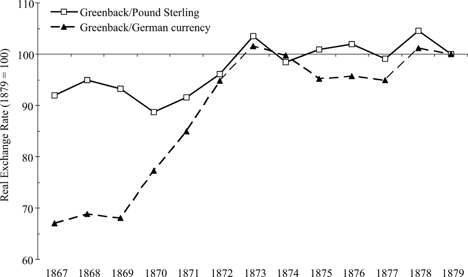
The relatively high value of the greenback during the late 1860s is consistent with significant buying pressure for U.S. securities that drove down yields on government bonds. Simon concluded that the strong demand for U.S. bonds at this time was due to a flight to security around the time of the Austro-Prussian war, the depressed state of European business activity, and the prevailing low interest rates available on the Continent. He cites contemporary estimates that U.S. government bonds held in Germany doubled from $250,000,000 in 1866 to $500,000,000 by the summer of 1868. Simon suggested that the subsequent search for yield by Continental investors led them to divert more funds to U.S. railroad investments and short-term capital in the form of call loans in New York. The Franco-Prussian War in 1870 caused a hiatus in negotiations of new loans. Nonetheless, the booming German economy absorbed much of its domestic capital available during the 1871–1873 period.Footnote ⁴⁰ The relaxation of German laws in 1870, leading to massive growth in the number of joint-stock firms in Germany, was undoubtedly a major impetus for investors there to focus on local firms rather than opaque U.S. railroads thousands of miles away.Footnote ⁴¹

Simon concludes that Continental investors began to prefer short-term call loans around this time as investors became increasingly wary of new railroad debt. His conclusion is based on anecdotal and quantitative evidence. As evidence, consider that the difference between Simon's estimate of capital imports (based on balance of payments data) and Frank Graham's estimate (based on long-term loans floated) peaks in 1872.Footnote ⁴² This suggests that Continental capital did not dry up because the boom ended, but because investors shifted to shorter duration exposure.

Kindleberger's story suggests that the indemnity payments stimulated the German economy, leading German investors to buy up assets (in Germany and elsewhere), which became overvalued by this pressure. If so, the net effect was not enough to drive up the real value of the greenback relative to the German currency. During the years of the indemnity payments the German currency became less and less undervalued relative to the greenback. In particular, this trend begins in 1870, prior to the indemnity payments. This puzzle can be resolved if we allow that investments flowed into Germany, bidding up the real value of the currency as soon as the capital markets opened up in 1870.Footnote ⁴³ It does not appear consistent with a story of flush German investors bidding up U.S. railroad investments indiscriminately. The floating greenback did not insulate the economy from the German economy, yet the German stimulus did not appear to dominate the effects on U.S. asset markets, in any case.Footnote ⁴⁴

Simon, in fact, presents evidence that U.S. bond issuers found Germany a difficult environment by 1872, as it was difficult to compete with newly available German investment opportunities. At the same time, German investors became less receptive to U.S. railroads in absolute terms. Simon cites a survey of German bankers from the first quarter of 1873, documenting that the bankers were very pessimistic about sizeable amounts of German capital becoming available for U.S. railroads. The survey concluded that “Doubtless the failure of a few properties had affected the values of the perfectly sound ones,” which is exactly the predicted effect of information asymmetry. Similarly, the American consul in Frankfurt observed in December 1872 that German investors “… can no longer be relied upon as a market for the securities of the railroad, cities, or even the states of the Union. So many railroad corporations have failed to pay their interest coupons … the buyer now considers everything American uncertain.”Footnote ⁴⁵

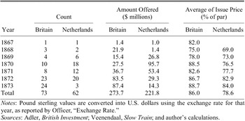
Detailed data on railroad bond offerings in Britain and the Netherlands for this period are available for analysis. Offerings in the Netherlands are taken as a proxy for offerings to all Continental investors, as many bonds were offered in several locations simultaneously. Table 5 displays summary information on offerings from 1867–1873 as collected by Dorothy Adler and Augustus Veenendaal.Footnote ⁴⁶ Several conclusions can be drawn from the table. Offerings in both countries were relatively small in the late 1860s but picked up sharply by 1870. The Dutch appear to have dropped out of the market by 1873, with offering amounts declining each year after 1870. The British, on the other hand, appear to have increased offerings in the last two years of the period. The final two columns of the table can be used to infer the quality of debt being offered in the two countries. Although both countries show a trend of increasing offering prices (and hence declining yields), the average issue price of bonds offered in the Netherlands is always lower than the price of bonds offered in Britain. Dutch investors were offered bonds with lower prices and higher yields than British investors were offered at the same time.

Table 5

U.S. RAILROAD BONDS OFFERED IN BRITAIN AND THE NETHERLANDS, 1867–1873

Notes:

Pound sterling values are converted into U.S. dollars using the exchange rate for that year, as reported by Officer, “Exchange Rate.”

Sources:

Adler, British Investment; Veenendaal, Slow Train; and author's calculations.

Further evidence on European bond holdings suggests that German and Dutch investors had put money into lower quality railroads. Contemporary estimates from late 1874 indicate that 25 percent of all U.S. railroad bonds were in default, but 40 percent of bonds held by European investors were in default. The distribution of defaults grew more lopsided as the situation unfolded. By the start of 1876, 14 percent of railroad bonds held in the United States were in default but 65 percent of foreign holdings had defaulted. Within the set of foreign investors, European investors fared much more poorly than British investors. Simon provides estimates that interest payments had been suspended on 9 percent of bonds held by Dutch investors (by face value) as of October 1873; by January 1874, over 43 percent of Dutch holdings by dollar value were in default, and over 10 percent more were expected to default.Footnote ⁴⁷

I conclude from the data that lower quality, riskier bonds were offered in the Netherlands, but that bonds offered in Britain were higher quality. Moreover, offerings to Dutch investors declined in the years before the crisis, suggesting that funding of long-term debt for lower quality, riskier railroads had dried up in the years immediately prior to the crisis. Overall capital flows did not decline as precipitously, as British investors displayed an increasing appetite for high quality railroad debt until the crash. Dutch investors had recognized in the late 1860s that they were purchasing risky bonds and priced them well below par to compensate for that risk. By the early 1870s they had perhaps learned that the risks were larger than initially expected, the returns might have been lower than initially expected, frauds were perpetrated by both American and Dutch interests, and that shorter duration exposure to U.S. railroads was prudent.Footnote ⁴⁸

Acceptable theories of the crisis should also account for the timing of events in Europe and the United States. Kindleberger suggests that the catalyst for the Vienna crash in May 1873 was underwhelming turnout for the Vienna Exposition, which opened on the first of the month. It is possible that expectations may have been reevaluated after the Exposition opened, but a focus on railroad distress in the United States seems a more compelling explanation. Continental investors held substantial amounts of U.S. bonds, many of which appear to have been low quality. Further, Continental investors were disadvantaged by the distance from and opacity of the railroads they funded. Any suspicion that the relevant firms were fraudulent, distressed, or otherwise impaired could have generated a widespread re-rating of railroad debt by European markets. As evidence of the bad facts and the introduction of uncertainty in the European marketplace in the early part of the year, consider the following April 1873 item from the CFC: “A damaging statement in regard to American railroad bonds in default for interest in Germany appeared this week in several of the daily newspapers, giving the following list of such bonds, viz.:

This was immediately contradicted as to the East Tennessee, Virginia and Georgia, the Port Royal, and the Oregon and California roads, by their officers or financial agents …”Footnote ⁴⁹

Note that these bonds generally represent smaller railroads, for which information might have been difficult to find. The fact that some of the firms were in default, whereas others technically were not, added to the uncertainty facing investors attempting to calculate the risk of their holdings. It is likely that the deteriorating balance sheets of U.S. railroads, coupled with European's difficulty in sorting out precisely what was going on with their investments thousands of miles away, was a more important determinant of the Vienna crash than the Vienna crash was for U.S. markets.Footnote ⁵⁰