2 Background: Multi-objective reinforcement learning

In this section, we provide the necessary background information on multi-objective reinforcement learning with a focus on single-policy methods.

In reinforcement learning, the agent is faced with the problem of making decisions in unfamiliar and possibly dynamic environments. In many cases there is more than one objective. Objectives may be directly related or completely independent of each other, in which case the objectives can be combined into a single objective, then the problem can be considered as a single-objective problem and a policy with the ability to maximize the combined objective should be found. If the objectives are in conflict with each other, no policy can be found that maximizes the effectiveness of all objectives. So either one of the objectives should be preferred or a compromise should be made between them. In this case, there is usually not a single optimal policy, but there is a set of optimal policies (Vamplew et al., Reference Vamplew, Dazeley, Berry, Issabekov and Dekker2011). In the case of single-objective reinforcement learning, the overall goal is to learn the optimal decisions in order to maximize a single numerical reward. These decisions are essentially actions that must be taken in specific situations in the environment. This environment is usually defined using a mathematical framework called the Markov decision process (Sutton & Barto, Reference Sutton and Barto1998). Reinforcement learning is a way to solve Markov decision problem by learning the optimal policy through interaction with the environment which results in the maximum possible reward in the long run. There is always at least one policy that is better or equal to other policies. The superiority of one policy ( $\pi $ ) over another ( ${\pi}^\prime$ ) is measured by the expected return of each.

To estimate the value of the agent being in a certain state or the value of the agent performing a particular action in a particular state, value functions are used which are functions of state-action pairs. The optimal value function for state s and the optimal value function for action a in state s are as follows:

(1) \begin{equation} V^*(s)={\mathop{\max }_{\pi } V^{\pi }\ }(s)\end{equation}

(2) \begin{align} Q^*(s)={\mathop{\max }_{\pi } Q^{\pi }}(s,a)\\ \nonumber\end{align}

During the learning process, the agent updates the value functions by receiving rewards to eventually learn the optimal policy. The Q-Learning algorithm was introduced by Watkins (Reference Watkins1989). In this algorithm, a table consisting of state-action pairs (s, a) is stored, each element of which contains an estimated value of $Q^*(s,\ a)$ . Q-values are updated according to the following formula:

(3) \begin{equation}Q_{t+1}(s,\ a)\leftarrow Q_t(s,\ a)+{\alpha }_t\ \left[R(s,\ a)+\gamma {\rm \ }{\mathop{\max }_{a^\prime} Q_t\ }(s^\prime,a^\prime)\ -\ Q_t(s,\ a)\right]\end{equation}

In the above formula $\ {\alpha }_t \varepsilon{\rm \ }\left[{\rm 0,1}\right]$ is the learning rate at time t. In each learning episode, the actions are selected according to a specific action selection strategy, and the agent goes to a new state in the environment and receives the corresponding reward, and the Q-value is updated according to the above formula. This process continues until the Q-values converge or for a certain number of episodes. If all elements of the Q-table (state-action pairs) are visited infinitely and the appropriate learning rate is selected, the estimated values of Q will converge to the optimal values (Tsitsiklis, Reference Tsitsiklis1994). In fact, the condition of convergence can be met when the difference between two updates of the same Q-value related to a specific state-action pair does not exceed a small threshold or algorithms reaches a predefined number of episodes (Sutton & Barto, Reference Sutton and Barto1998).

To model a multi-objective problem as a reinforcement learning problem, we need to define the Multi-Objective Markov Decision Process (MOMDP) in which the reward is not a single scalar but a vector of rewards. The only difference between the standard and Multi-Objective Markov Process definition is in the definition of the reward function such that for a problem with m objectives it is defined as a vector with m dimensions as follows in which $R_i(s,\ a,\ s^\prime)\ $ is the single scalar reward related to the $\textit{i}^{th}$ objective:

(4) \begin{equation}{R}({s}, {a}, {{\rm s}'}) \rightarrow {{\mathbb R}}^m \end{equation}

(5) \begin{align} R(s,\ a,\ s^\prime) = (R_1(s,\ a,\ s^\prime),\ R_2(s,\ a,\ s^\prime),\dots ,\ R_m(s,\ a,\ s^\prime))\\[3pt] \nonumber\end{align}

Expected return is also defined in terms of the vectors:

(6) \begin{equation} R_t = (R_{t{\rm 1}}{\rm ,\ }R_{t{\rm 2}}{\rm ,\dots .},R_{tm}{\rm )}\end{equation}

Each $R_{ti}$ represents the expected return for each objective which is equal to the sum of the rewards for that objective over time and is equal to following formula:

(7) \begin{equation} R_{ti}=\sum\nolimits^{\infty }_{k=0}{{\gamma }^kr_{t+k+1}}\end{equation}

Here $r_t\ $ is the reward received at time t and $0 \leq \gamma \leq 1$ is the discount factor that determines the relative importance of future rewards. The closer $\gamma $ is to 1, the more important the future rewards will be. In the case of finite problems, the sum of the observed rewards is taken into account, and in the case of infinite problems, the infinite sum is taken into account. This definition applies to both episodic and continuous problems. Episodic problems have a final state that ends the episode. After reaching the final state, the environment returns to the initial state. Continuous problems never end because there is no end to them and are not separable into smaller episodes and therefore do not have a final state, so $\gamma $ cannot be equal to one (Sutton & Barto, Reference Sutton and Barto1998).

In Multi-objective reinforcement learning the goal is to solve the Multi-Objective Markov Decision Process (MOMDP) problem and find a policy to maximize the cumulative vectorial reward, which is the reward gained during execution or as expected return.

The value function for the state s and under the policy $\pi $ is defined as follows (Moffaert, Reference Moffaert2014):

(8) \begin{align} V^{\pi }(s) &= {{\mathbf{E}}}_{\pi }\left[R_t\ \right|\ S_t=s,\ A_t=a\ ] \nonumber\\[3pt] & = {{\mathbf{E}}}_{\pi } \left[\ \sum\nolimits^{\infty }_{k=0}{\sum\nolimits^m_{i=1}{{\gamma }^kr_{ti+k+1}}} \mid S_t=s\ ,\ A_t=a\ \right] \end{align}

In above formula ${{\mathbf{E}}}_{\pi }$ represents the value of the random variable given that the agent follows policy $\pi $ . In fact, the value function is calculated as the expected vectorial return that the agent receives if it starts from state s and selects actions according to the policy $\pi $ .

The most common measure of policy optimality is called Pareto dominance and is defined as follows (Moffaert, Reference Moffaert2014):

The policy ${\pi }_1\ $ is strictly Pareto dominates ${\pi }_2$ ( ${\pi }_2 \succ {\pi }_1\ $ ) if it is strictly better on at least one objective of policy $\ {\pi }_{2\ }$ , and at the same time it is not strictly worse on the other objectives in all states. The policy ${\pi }_1$ weakly Pareto dominates ${\pi }_2$ ( ${\pi }_2 \succcurlyeq $ ${\pi }_1$ ) when there is no objective that for all states, $V^{{\pi }_1}(s)$ is better than $V^{{\pi }_2}(s)$ . The policies ${\pi }_1$ and ${\pi }_2$ are incomparable if $V^{{\pi }_1}(s)$ does not Pareto dominate $V^{{\pi }_2}(s)$ for all states and vice versa. The policy ${\pi }_1$ is non-dominated by the policy ${\pi }_2$ if it either Pareto dominate policy ${\pi }_2$ or is incomparable with that policy. Any solution that is dominated by another solution has less value and the dominant solution is preferred. Thus, Pareto optimal solutions or policies are those that are either strictly dominant or incomparable to any member of the solution set. If this procedure is applied to a set of possible solutions, a non-dominated set of solutions is obtained, which is called the Pareto front.

Multi-objective reinforcement learning algorithms are divided into two categories: single-policy and multi-policy. In this paper, since our proposed method belongs to first category, we will not discuss multi-policy algorithms and focus only on the single-policy algorithms. In the following subsections we will introduce the most common and noteworthy single-policy algorithms.

2.1 Linear scalarization

Single-policy algorithms are similar to single-objective reinforcement learning algorithms in that they learn only one optimal policy. In multi-objective algorithms, however, there are usually more optimal policies on the Pareto front, and it must be specified for the algorithm which of the optimal policies is preferable (Vamplew et al., Reference Vamplew, Dazeley, Berry, Issabekov and Dekker2011). One way to prioritize is to use a scalarization function that converts the reward into a numerical value. This leaves us with only one value function that can be achieved by one or more optimal policies. Scalarization functions are defined as follows:

(9) \begin{equation} v_w\ = f(v,w)\end{equation}

In the above formula, f is a scalarization function that converts the vector v to a scalar. These functions usually use the weight vector w to determine the relative importance of the objectives. The main drawback of single-policy algorithms is that the preference of objectives must be decided in advance. Weight changes related to objectives can cause a decrease in one objective to a very small extent but a significant increase in another objective. In fact, depending on the nature of the Pareto front, small changes in weights can cause large changes in the policy being learned, and vice versa (Vamplew et al., Reference Vamplew, Yearwood, Dazeley and Berry2008). The linear scalarization function calculates the inner product of the weight vector w and the value vector $V^{\pi }$ obtained from the learned value function:

(10) \begin{equation}V^{\pi }_w = w. V^{\pi } \end{equation}

Each element of w is a real number in the range [0,1] that indicates how much a value associated with each objective will contribute to the scalarized value. All of the weights must be positive and sum to 1. For representing the value functions in single-objective learning, the agent stores a table of values of Q(s, a) that represents the expected cumulative discounted reward associated with each pair of state s and action a in the environment. These values of Q(s, a) are updated over time using formula (3). In a multi-objective environment to learn a single-objective policy, the agent stores a Q-vector for each pair of state and action. Each Q-vector contains a Q(s, a) value for each objective. Q-vectors are updated separately for each element. For example, objective O of the Q-vector is updated using the following formula, which is used for multi-objective Q-Learning and is called the bootstrapping rule:

(11) \begin{equation}Q_o(s,\ a)\leftarrow Q_o(s,\ a)+ {\alpha }_t\ ({{\mathbf r}}_o+\gamma {\rm \ }{\mathop{\max }_{f(Q(s^\prime,a^\prime),w)} Q_o\ }(s^\prime,a^\prime)-\ Q_o(s,a))\end{equation}

In the above formula ${{\mathbf r}}_o$ is o ${}^{th}$ element of the immediate reward vector and ${\mathop{\max }_{f(Q(s^\prime,a^\prime),w)} Q_o\ }(s^\prime,a^\prime)$ regarding the scalarization function f and the weight vector w gives the maximum scalarized value in the Q vector (Moffaert, Reference Moffaert2014).

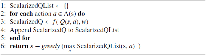
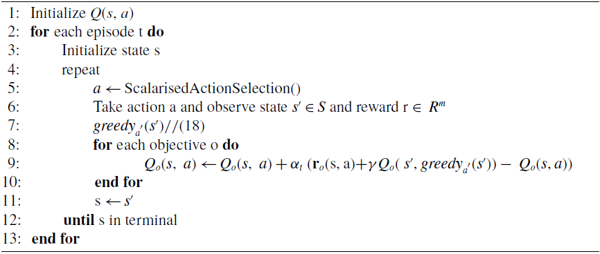
In order to describe the algorithm, the mechanism of action selection must first be specified. The exploration is done as ε -greedy, which ε indicates the randomness of the action selection and 1- ε the best action based on the greatest value of the value function and the corresponding Q-values to go to the next state. In order to be able to determine the best action to go to the next state in a multi-objective environment, the values of the Q vectors must be converted to a scalarized value. The action selection algorithm is presented in Algorithm 1. The scalarization function f which is linear, calculates the linear combination of the values of a vector with respect to the weight vector w. In fact, in the framework of the multi-objective reinforcement learning algorithm shown in Algorithm 2, it operates according to (12) and eventually based on (13) the action that has the highest weighted sum, that is, the sum of its Q-values in the state s for all objectives is greater than all other actions, is selected as the next action:

(12) \begin{equation}\mathrm{ScalarizedQ}(s,a) = (s,a). w = \sum^m_{o=1}{Q_o(s,a)}\ .w_o \\\end{equation}

(13) \begin{align}{greedy}_{a'}(s) = {\mathop{{\rm m}a{\rm x}}_{a'} \mathrm{ScalarizedQ(s,}\ a'{\rm )\ }\ }\\ \nonumber\end{align}

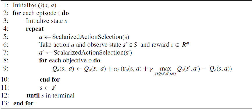
To start the algorithm, the agent is in an initial state in each episode. In the next step, the agent selects an action and by adopting that action, observes the state to which it has gone and its reward vector. Using the action selection function, and according to the observed state s $^{\prime}$ , action a $^{\prime}$ is selected and used to update the Q-table of each objective. Then for all objectives according to the reward vector obtained and the maximum scalarized value, the Q vector is updated by the scalarization function f. The agent then goes to the next state and these operations are repeated until it reaches a final state and a new episode begins. The algorithm terminates after convergence. The pseudo-code of the algorithm is given in Algorithm 2.

In the linear scalarization method, the relative importance of the objectives to each other is specified by w and should be determined before starting the learning process. From a convergence point of view, since this algorithm is based on Q-Learning and only the scalarization function is added as a mechanism for selecting action, it converges in exchange for a certain number of episodes. More theoretical details are available in Sutton and Barto (Reference Sutton and Barto1998). The Linear scalarization has simplicity and fair speed, but various articles have mentioned that this method is only able to find policies that are in the convex region of the Pareto front (Vamplew et al., Reference Vamplew, Yearwood, Dazeley and Berry2008; Roijers et al., Reference Roijers, Vamplew, Whiteson and Dazeley2013). Therefore several researchers have proposed the use of nonlinear scalarization methods. The following subsections will review some of these nonlinear approaches to scalarization.

Algorithm 1

Scalarized Action Selection (Moffaert, Reference Moffaert2014)

Algorithm 2

Scalarized Multi-Objective Q-learning (Moffaert, Reference Moffaert2014)

2.2 Threshold lexicographic Q-learning

The TLQ-Learning algorithm uses a combination of thresholding and lexicographic ordering to guide the learning process. This algorithm has the ability to define a threshold value for each objective, which is defined depending on whether the objective should be maximized or minimized. Therefore, this method is mainly suitable for situations where one objective should be maximized and at the same time constraints should be applied to other objectives. After reaching the threshold value on one objective, the agent does not continue to advance on that objective and optimizes the other objective (Gabor et al., Reference Gabor, Kalmar and Szepesvari1998).

Due to the limitations on the objectives, the definition of the value function in the action selection mechanism is defined as follows:

(14) \begin{equation} {CQ(s,a)}_i= {\min\ }({CQ(s,a)}_i,C_i)\end{equation}

The threshold value for i ${}^{th}$ objective is denoted by $C_i$ . If we have m objectives, we usually set a limit on all of them except the last objective, that is, $C_m = \infty$ . Ordering objectives also leads to ordering policies. To compare the policy $\pi $ with the policy ${\pi }^\prime$ , we first look at the first objective and choose the policy that works best for that objective. If the cumulative reward of the first objective is the same for both policies, we must compare the second objective, and so on. If the policies have the same value on all objectives, we can choose one of them arbitrarily. Given that most objectives are constrained to their threshold values, the cumulative reward for these goals will be the same for many policies. Therefore a policy can be chosen that satisfies all constraints and maximizes the last objective (Gabor et al., Reference Gabor, Kalmar and Szepesvari1998).

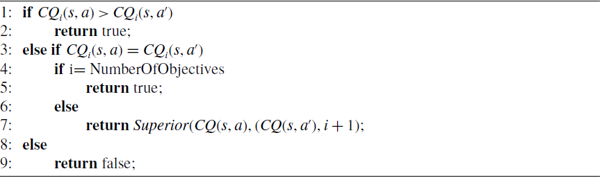
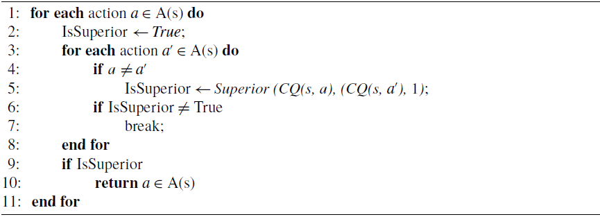
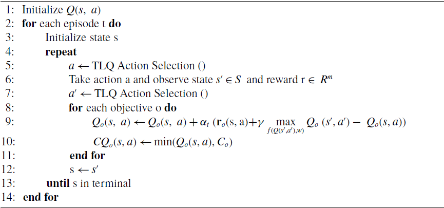
The TLQ-Learning algorithm is presented by changing the action selection mechanism of Algorithm 2. Therefore, we must first define its action selection algorithm. To do this, we need to define the Superior algorithm, which compares two operations and their value function in the form of Algorithm 3. Then we can define an action selection algorithm (Algorithm 4) that actually greedily selects action a in state s if it is superior to all other actions according to Algorithm 3. Finally, by defining these two algorithms, the TLQ can be presented in Algorithm 5. The difference between this algorithm and the Linear Scalarization is the use of a different action selection algorithm and the addition of the calculation of ${CQ}_i(s,a)$ in line 10, which is used to select the action.

The results of experiments on the Linear Scalarization and TLQ-Learning algorithms in Issabekov and Vamplew (Reference Issabekov and Vamplew2012) indicate that in problems whose structure is suitable for the TLQ-Learning method, since it can detect policies located in concave regions, it outperforms the Linear Scalarization method which is unable to detect them. The convergence of the algorithm cannot be proved formally due to nonlinearity of the scalarization function and the quality of the test results should be relied upon.

Algorithm 3

Superior (Vamplew et al., Reference Vamplew, Dazeley, Berry, Issabekov and Dekker2011)

Algorithm 4

TLQ Action Selection

2.3 Chebyshev scalarization

This algorithm is based on the $L_p$ norm. $L_p$ calculates the distance between the point x and the utopian point $z^*$ in multi-objective space. $L_p$ is defined to measure the distance of the value of the objective function f from $z^*$ as follows. Note that f is a function of solution x for each objective o:

(15) \begin{equation} L_p\ (x)={\left(\sum^m\nolimits_{o=1}{w_o}{\left|f_o(x)-\ z^*_o\right|}^p\right)}^{1/p}\end{equation}

where m is the number of objectives and $w_o$ is the weight of the objective o. Also, p is a number in the range of $[1, \infty]$ . If ${p} = \infty$ , the $L_p\ $ norm is called the weighted $L_\infty$ or the Chebyshev norm and is defined according to the following formula:

(16) \begin{equation} L_\infty(x) =\ {\mathop{\max }_{o=1\dots m} w_o\ }\left|f_o(x)-\ z^*_o\right|\end{equation}

by replacing the function $f_o(x)$ with the value of Q associated with each objective and pair of state and action, the $L_\infty$ criterion can be used as a scalarization function in the action selection mechanism in multi-objective learning. Therefore, the scalarized value of Q for state s and action a is defined as follows:

(17) \begin{equation}\mathrm{ScalarizedQ}\ (s,a) = {\mathop{\max }_{o=1\dots m} w_o\ }\left|Q(s,a,o)-\ z^*_o\right| \end{equation}

by substituting (17) instead of the scalarization function f in Algorithm 1, the action selection mechanism of the Chebyshev algorithm can be defined. The difference is the choice of the greedy action, which in the standard mode and in Algorithm 1 is the action with the maximum value, but here is the minimum value and is defined as follows:

(18) \begin{equation}{greedy}_{a^{\prime}} (s) = {\mathop{\min }_{a'} {\rm ScalarizedQ(s,}\ a'{\rm )\ }\ } \end{equation}

The goal is to get as close as possible to the utopian point $z^*$ , so we must choose the action that has the shortest distance to that point. During the learning process, the ideal point $z^*$ is constantly updated with the best value of each objective up to that point plus a constant value of $\tau \in {\mathbb R}$ and guides the learning process towards the optimal solution. This update is added to Algorithm 2. Finally, assuming that Algorithm 1 and the corresponding action selection mechanism use (17) instead of f in its line 3, the Chebyshev algorithm is defined as Algorithm 6.

Algorithm 5

TLQ-Learning

Algorithm 6

Chebyshev Scalarized Q-Learning Moffaert et al., Reference Moffaert, Drugan and Nowé2013

As any other algorithm that uses nonlinear function, the Chebyshev nonlinear function lacks the property of addition. Therefore, the Bellman equation is not established for it and it cannot be formally and theoretically proved that the Chebyshev function in combination with a learning algorithm will converge to an optimal policy (Moffaert, Reference Moffaert2014). However, in practice, performance and results of the experiments are reported to be very good and satisfactory. As stated by the original paper this approach can find policies regardless of their location and provides better coverage solutions on the front. Also it is less dependent on the weight of the objectives compared to methods that use the Linear Scalarization and due to the nonlinearity of the function used policies that are in the non-convex region can be found (Moffaert et al., Reference Moffaert, Drugan and Nowé2013).

3 Proposed model: TOPSIS Q-learning

In both multi-criteria decision-making and multi-objective reinforcement learning, prioritizing objectives and solutions is the responsibility of the user or so-called decision-maker and plays an important role in the decision-making process. In fact, by determining preferences by the user, the relative importance of objectives to each other is specified. In literature there are three ways to express preferences: prior, posterior, and interactive. Specifically in the prior method, the user sets preferences before the decision-making or learning process (Moffaert, Reference Moffaert2014). Most of the previous methods include priorities in the form of parameters in the problem, which leads the search process to a solution that satisfies these priorities. In this regard, similar to the approach taken by all the methods reviewed in Section 2 a scalarization function is used which reduces the multi-objective problem to a single-objective problem by considering the user’s preferences as a constraint in order to maintain optimality. As mentioned previously, a scalarization function is a function that converts a vector to a scalar according to a given weight vector. When the user is already aware of the priorities of the objectives in the decision-making problem, there is no need to estimate the Pareto front of the optimal solutions and the weight vectors specifies the compromised or trade-off solutions that somehow specified before the execution of the algorithm by the user. So there is an overlap between the decision-making process and multi-objective reinforcement learning. In the following, we will see how the agent in the decision-making process in the action selection mechanism can use the multi-criteria decision-making method.

We are looking for optimal solutions in MCDM problems. Although there is often no optimal solution due to conflicting objectives or criteria, an optimal solution, also called the ideal solution, is a solution in which the value of each objective is maximized simultaneously. The ideal solution is not actually achievable, but can be used as a guide for evaluating other solutions. MCDM is divided into two sub-categories: Multi-Objective Decision Making (MODM) and Multi-Attribute Decision Making (MADM). MODM includes problems in which the decision space is continuous and MADM deals with problems which have discrete decision space. In this paper, as our decision space in action selection mechanism in MORL is discrete so we use MADM to aid the decision process. The ideal solution in MADM is a hypothetical alternative whose Cartesian product consists of the values of each criterion with the highest preference in the decision matrix.

To reach a trade-off model finding a non-dominated solution which is close to the ideal solution is necessary. A non-dominated solution (also known as a Pareto-optimal solution) is a feasible solution where there is no other solution that could improve on an objective without performing worse on at least one other objective. A non-dominated solution is called a preferred solution when it is selected as the final solution using decision-maker’s preference information (Hwang & Yoon, Reference Hwang and Yoon1981).

There are some methods for MADM which process the criteria or attributes to reach a solution. Two major approaches are non-compensatory and compensatory models. Non-compensatory models are simple to use but lack ability to trade-off between criteria, that is, a decline in the value of one criterion cannot be offset by an improvement in the value of another. In contrast, compensatory models allow trade-offs between criteria. Each alternative in decision matrix with multiple criteria is assigned to a single number or score. There are three approaches to calculate this number and appropriate alternative. (1) Scoring model which selects an alternative with highest score using various weighting methods. (2) Concordance model which performs pair-wise comparisons of alternatives in order to rank them based on concordance. (3) Compromising model which selects alternative based on its closeness to the ideal solution. Since compromising model takes advantage of the concepts of ideal, non-dominated and Pareto-front solutions which are crucial concepts in MORL as well, so it seems we could apply that to assist the agent in decision-making process in action selection mechanism. One of the famous methods of this model is TOPSIS which uses ideal solution concept in its core to rank alternatives (Hwang & Yoon, Reference Hwang and Yoon1981).

3.1 TOPSIS method

Since we will use TOPSIS in the proposed model, here we introduce this multi-criteria decision-making method that was introduced in 1981 by Hwang and Yoon (Reference Hwang and Yoon1981). In this method, the m alternatives are evaluated by n criteria. In fact, a decision matrix with the form of n $\times$ m is constructed. This method is basically based on the two concepts of positive and negative ideal solution. This means that the alternative chosen must have the shortest distance from the positive ideal solution (best possible case) and the longest distance from the negative ideal solution (worst possible case). To solve the problem after forming the decision matrix, the following six steps must be followed (Hwang & Yoon, Reference Hwang and Yoon1981):

1. 1. Normalizing the decision matrix X: The matrix is normalized in the form of ${(x_{ij})}_{m\times n}$ as follows:

   (19) \begin{align}r_{ij} &= \frac{x_{ij}}{\sqrt{\sum^m_{k=1}{x^2_{kj}}}} \textit{, i}=\textit{1,2,\dots ,\,m, j}=\textit{1,2,\dots ,n} \nonumber\\\textit{R}&= {(r_{ij})}_{m\times n}\end{align}

2. 2. Calculating the weighted normalized decision matrix: We multiply the normalized decision matrix of the previous step in the diagonal matrix of weights ${{\rm W}}_{{\rm n}{\rm \times }{\rm n}}$ in the following order:

   (20) \begin{align}V &= R \times W_{n\times n} \nonumber\\[3pt] v_{ij} &= r_{ij} \cdot w_j, i=1,2,\dots ,m, j=1,2,\dots ,n\nonumber\\[3pt] w_j &= W_j/\sum\nolimits^n_{k=1}{W_k}, {j=1,2,\dots ,n,} \sum\nolimits^n_{k=1}{w_i} =1\end{align}

3. 3. Determining the positive ideal solution and the negative ideal solution:

   Positive ideal solution ( $v^+_j$ ) = vector containing the best values of each criterion of the matrix V.

   Negative ideal solution ( $v^-_j$ ) = vector containing the worst values of each criterion of the matrix V.

   The best values for positive criteria are the largest values and for negative criteria are the smallest ones, and the worst values for positive criteria are the smallest values and for negative criteria are the largest ones.

4. 4. Calculating the distance between the alternatives and the positive and negative ideals: To do this, the Euclidean distance of each alternative from the positive ideal and the negative ideal solutions must be calculated in the following order:

   (21) \begin{align}d^+_i = \sqrt{\sum\nolimits^n_{j=1}{{(v_{ij}-v^+_j\ )}^2}}, {i=1,2,\dots ,m}\\d^-_i = \sqrt{\sum\nolimits^n_{j=1}{{(v_{ij}-v^-_j\ )}^2}}, {i=1,2,\dots ,m}\nonumber\end{align}

5. 5. Determining the relative similarity of each alternative to the ideal solution:

   (22) \begin{equation} {cl}_i = \frac{d^-_i}{d^-_i+\ d^+_i}\end{equation}

6. 6. Ranking: the alternative with a larger cl is preferred.

If distance measure in TOPSIS is defined by the Manhattan distance instead of the Euclidean distance then the Simple Additive Weighting (SAW) method will be a special case of TOPSIS. For proof let assume the distance between $A_i$ and $A_k$ is defined by following formula:

(23) \begin{equation}d_{ik} = \sum\nolimits^n_{j=1}{\left|v_{ij}-v_{ij}\right|}\ \mathrm{i}, \mathrm{k} = 1,2,\dots , \mathrm{m}\ \mathrm{i} \neq \mathrm{k }\end{equation}

As Manhattan distance has the following relationship:

(24) \begin{equation}d^*_i + d^-_i = d^-_* = {K}, i = 1,2,\dots ,{m} ({K} > 0\ \textrm{and}\ \textrm{Constant})\end{equation}

So alternatives with the shortest distance to the positive ideal solution have the longest distance to the negative ideal solution. And for ${i} = 1,2,\dots ,{m}$ relative closeness can be defined as $C^*_i = d^-_i/d^-_*$ . If alternative $A^+$ is defined by $A^+=\{\ A_{i\ }| {\mathop{\max }_{} C^*_i\ } \}$ and finally it is proved (Yoon, Reference Yoon1980; Hwang & Yoon, Reference Hwang and Yoon1981):

(25) \begin{equation}A^+=\{\ A_{i\ }| {\mathop{\max }_{i} \sum\nolimits^n_{j=1}{v_{ij\ }}\ } \} = \{ A_{i\ }| {\mathop{\max }_{i} C^*_i\ } \}\end{equation}

SAW method functions exactly like Linear Scalarization to select an alternative. Both choose an alternative which has the maximum average outcome. As we stated above if we replace Euclidean distance measure with Manhattan distance, TOPSIS will be converted to SAW or weighted sum model. The critical difference between these two measures is trade-off which explained in Hwang and Yoon (Reference Hwang and Yoon1981), Keeney and Raiffa (Reference Keeney and Raiffa1976) MacCrimmon and Toda (Reference MacCrimmon and Toda1969), and MacCrimmon and Wehrung (Reference MacCrimmon and Wehrung1977) and we will review it here.

Ratio of the change in one criterion that exactly negates a change in another criterion is called trade-off or marginal rate of substitution (MRS). Contours on a given value function are called indifference curves. It is assumed each alternative located on an indifference curve is preferred equally by a decision-maker. Given the indifference curves the trade-off or MRS at any point is equal to negative reciprocal of the slope at that point. If indifference curve is defined by ${\rm f}(v_1,v_2)=\textrm{c}$ where f is a value function and c is a constant and $v_{1\ }$ and $v_{2\ }$ are coordination of a point through which curve passes. To calculate MRS we have the following:

(26) \begin{equation} \lambda = - \frac{{dv}_1}{{dv}_2} |_{{\rm (}v_{1}{\rm ,\ }v_{2\ }{\rm )}} = \frac{\partial f}{{\partial v}_2}/\frac{\partial f}{{\partial v}_1} |_{{\rm (}v_{1}{\rm ,\ }v_{2\ }{\rm )}}\end{equation}

Since value function of SAW or TOPSIS with Manhattan distance measure is equal to ${\rm f}(v_1,v_2)=v_1+v_2$ , MRS is obtained by $\lambda =1$ . So it can be concluded that trade-off (MRS) in SAW is constant between criteria and indifference curves are straight lines with the slope of −1. This type of trade-off considers local MRS as the global one as well.

To calculate trade-off in TOPSIS with Euclidean distance measure we have to calculate $\lambda $ using value function:

(27) \begin{equation}f (v_{1}, v_{2\ }) = \frac{d^-_i}{d^-_i+\ d^*_i} = \textrm{c} = \frac{\sqrt{{(v_{1-\ }v^-_1)}^2+\ {(v_{2-\ }v^-_2)}^2\ }}{\sqrt{{(v_{1-\ }v^-_1)}^2+\ {(v_{2-\ }v^-_2)}^2}+\ \sqrt{{(v_{1-\ }v^*_1)}^2+\ {(v_{2-\ }v^*_2)}^2\ }}\end{equation}

(28) \begin{align} \lambda = \frac{{d^-_i}^2(v^*_2-\ v_{2\ })+\ {d^*_i}^2 (v_{2\ }-\ v^-_2)\ }{{d^-_i}^2(v^*_1-\ v_{1})+\ {d^*_i}^2(v_{1\ }-{\ v}^-_1)} \\ \nonumber\end{align}

For the point at where distances to the positive and negative ideal solutions are the same (i.e. $d^*_i=\ d^-_i$ ) $\lambda $ and value function equal the following:

(29) \begin{equation} \lambda = \frac{\ v^*_2-\ v^-_2}{v^*_1-{\ v}^-_1}\end{equation}

(30) \begin{equation}{\rm c} d^*_i - (1 - \textrm{c}) d^-_i = 0, 0 < \textrm{c}< 1\end{equation}

As a conclusion in TOPSIS the property of diminishing MRS is in effect which allows trade-off between criteria more naturally and flexible than weighted sum method (and consequently the Linear Scalarization) that the MRS is a constant and doesn’t follow this property. Also for some specific values of relative closeness to the positive and negative ideal solutions ( $C^*_i$ ) indifference curves are convex or concave to the preference origin. The former is more common and the latter is suitable for situations in which decision-maker for any reason is inclined to negative ideal solution rather than positive one (MacCrimmon & Toda, Reference MacCrimmon and Toda1969; Hwang & Yoon, Reference Hwang and Yoon1981). Another advantage of using TOPSIS in our MORL model is that it recognizes the lack and not only the presence of criteria.

3.2 Using TOPSIS in the proposed model

In the proposed model, if we consider TOPSIS as an action selection function, the standard form of this function could be as follows:

(31) \begin{equation} topsisActionSelection\ (actions, C_1(s),\dots , C_N(s), w)\end{equation}

where actions are an array of alternatives to select, that is, the same agent’s actions, $C_1$ and $C_N$ are the criteria related to all actions in state s for the preference set 1 and preference set N respectively containing corresponding Q-values and weight preferences. That is, all weight preferences are given to the action selection function as decision criteria at once, and unlike other previous scalarization models, there is no need for the user to choose the weight preferences. w is the weight vector by which the relative importance of each of the decision criteria or weight preferences can be determined. Normally we define the TOPSIS weight vector in the uniform way (with equal weights sum to one). This function is called when the agent has to decide to select the next action. According to Section 3.1 the decision matrix is formed first, where actions are decision or selection alternatives and Q-values in state s related to different weight preferences are the decision criteria. Then steps 1 to 6 of TOPSIS Method (Section 3.1) are performed and the output of the function is the ranking of the alternatives, which is usually the alternative with the rank of 1 will be chosen. Hence the greedy action which is obtained from scalarization function is generated as follows:

(32) \begin{equation} {greedy}_a = {\mathop{\max }_{} Q_{i\ }(s,a)\ \ } i=1\dots n\end{equation}

Suppose that each of the decision criteria given to TOPSIS is a combination of objectives with different weights. In this case, each criterion can be defined as follows:

(33) \begin{align}C_j (s,a) &= {\mathop{\max }_{i} w_1Q_{1\ }(s,a),\dots ,w_iQ_i(s,a),\dots ,\ w_nQ_n(s,a)\ \ }\\[3pt] & \sum^n_{i=1}{w_i}=1 \nonumber\end{align}

Each criterion is denoted by $C_j$ and $\textrm{j}=1,2,\cdot,\textrm{m}$ is the number of criteria. The total weight of the objectives must also be equal to one. In fact, the objective that is most valuable is selected according to the state and action pair in Q table as well as its weight coefficient. Of course, this selection is updated and changed according to the change of Q-values in each episode. Also note that each of the criteria contains a different weight combination according to the objectives coefficients. In some cases, despite the use of single-policy and scalarization methods and the provision of weights before the start of the decision-making and learning process, the preferences for the user may not be completely definite or are subject to change. There has been some research on designing a framework that can include uncertainty and changes in the preferences of the objectives in the field of multi-objective reinforcement learning (Roijers et al., Reference Roijers, Zintgraf and Nowé2017, Reference Roijers, Zintgraf, Libin and Nowé2018, Reference Roijers, Zintgraf, Libin, Reymond, Bargiacchi and Nowé2020; Vamplew et al., Reference Vamplew, Issabekov, Dazeley, Foale, Berry, Moore and Creighton2017) and in this study we want to address this issue in a different way. The problem can be modeled with the help of TOPSIS as presented in the first version of the algorithm of our proposed model. As we will show in the following, a different weight combination of objectives can be created with each criterion to cover changes and uncertainty of user preferences. These weight combinations for each objective are slightly apart from each other (for example 0.1).

The user may also want to train and use the model for a specific set of weights. Each objective, that is, its Q table multiplied by related weight is given to the TOPSIS function as a criterion and finally TOPSIS algorithm carries out the operation to select the next action for the agent. Unlike the first version, which is weight-independent, the scalarization function of the second version must take into account the user’s preference weights. So the greedy action generated from scalarization function for the second version is presented as follows:

(34) \begin{equation} {greedy}_a = {\mathop{\max }_{i} w_iQ_{i\ }(s,a)\ \ } i=\ 1\dots n\end{equation}

3.3 TOPSIS Q-learning algorithm

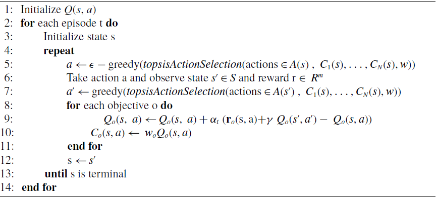
This algorithm is based on Q-Learning and its structure is similar to the Linear Scalarization, except that its action selection mechanism is replaced by TOPSIS. As mentioned earlier, in the first version of proposed algorithm, unlike other single-policy methods in which weights must be set as preferences by the user before starting the learning process, these weight combinations are automatically generated as decision criteria in the algorithm at once and simultaneously and do not need to be determined by the user, and with only one run and taking into account all these weight combinations, the solution is produced. These weights are used as Q-coefficients for the objectives to form weight preferences of the objectives associated with them. Each weight combination is considered as a decision criterion for TOPSIS so that the user can model the conditions of uncertainty and weight changes of objectives around their preferences over objectives. In the first version of the algorithm using the TOPSIS action selection mechanism, the values of the Q Table related to each objective in state s alongside corresponding weights are given to TOPSIS as a criterion for all actions in that state to select the optimal action (line 5 of Algorithm 7). Also, to update the Q table of each objective, the TOPSIS action selection mechanism is used, that is, the value of the Q table for each objective according to the received reward and towards the Q-value related to the optimal action of the next state, which is determined by TOPSIS for all objectives is updated (line 9 of Algorithm 7). An overview of the first version of the algorithm is given in the form of Algorithm 7.

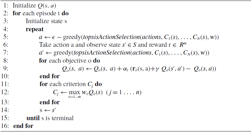
In the second version of the algorithm the agent invokes the TOPSIS function as the action selection mechanism when deciding to move to the next state. TOPSIS considers all criteria as shown in line 8 of Algorithm 8 while $\varepsilon$ -greedy selection. In fact steps 1 to 6 of Section 3.1 are performed and finally the alternative with a highest rank is selected as the preferred action and agent goes to the next state $s^\prime$ (line 9). In line 10 greedy function is applied on TOPSIS in state $s^\prime$ and action $a^\prime$ is selected to update the Q-Learning formula in line 11. The Q-values and criteria are then updated and the agent goes to the next state. The choice of learning and environment-related parameters will be discussed in Section 4. The second version of the algorithm is presented in Algorithm 8. The subtle distinction between criteria of two versions of algorithms is that the first version handles different combinations of weight preferences while the second one directly deals with the objectives. N in $C_N$ in Algorithm 7 refers to the number of combinations of weights and in Algorithm 8 it refers to the number of objectives.

Algorithm 7

TOPSIS Q-Learning – First Version

Algorithm 8

TOPSIS Q-Learning – Second Version

To prove the convergence, it should be said that although the algorithm is based on Q-Learning, but because the TOPSIS method is basically based on the concept of its distance function (i.e. calculating the distance of alternatives from the positive and negative ideal solution) and the distance function in TOPSIS is nonlinear and lacks additivity, so the Bellman equation does not hold for it. As a result, like other methods that combine nonlinear scalarization functions with Q- Learning, the convergence of the algorithm into an optimal policy is not theoretically provable and must rely on practical and experimental results.

In fact, using nonlinear scalarization functions such as Chebyshev, TLQ, etc. in combination with Q-Learning, the basic assumption in the Bellman equation, namely the property of additivity of returns, is no longer established. Therefore, there is no guarantee that the agent will converge to the optimal policy (i.e. in terms of numerical rewards during the episode). The question also arises as to whether the algorithm will converge at all in some cases where the agent meets a state again or the states and rewards are random. In general, to ensure convergence under such conditions, the agent must store the sum of the rewards it has earned so far in the current episode and in each state by adding that sum of rewards to the values of Q(s, a) and scalarization of the yielded sum in the action selection should be done. Also the decisions about Q-values should also be made based on the values of accumulated rewards and the current state (Geibel, Reference Geibel2006; Roijers et al., Reference Roijers, Vamplew, Whiteson and Dazeley2013).

4 Experiments and results

It is obvious that the research problem does not end with the presentation of the model and the model must be tested. The test is performed in different environments with parameters specific to that environment and specific configuration related to the algorithm to achieve the highest possible efficiency or the optimal solution in the solution space. In order to evaluate multi-objective reinforcement learning algorithms, the solution obtained online may be satisfactory, but not offline, and vice versa. An algorithm that is suitable for one environment may be unsuitable and ungeneralizable for another environment. Single-policy algorithms are suitable for online learning. The effectiveness of online learning can be assessed in two ways: the hypervolume of the accumulated rewards and regret measure. To use the regret measure, the Pareto front of the problem or the optimal policy must be known in advance. For many problems where the optimal policy is unknown, the hypervolume of the accumulated reward can be calculated without knowing the optimal policy. In situations where we are not aware of the Pareto front of the problem, the online hypervolume measure is the best option, but if we know the solution, the regret measure can provide more accurate information (Vamplew et al., Reference Vamplew, Dazeley, Berry, Issabekov and Dekker2011). However, the most common evaluation method in most papers is the hypervolume measure.

In the definition of hypervolume, we can say that by considering a reference point r over which the whole Pareto front (solution set S) or our estimation of the Pareto front dominates, the space between r and the Pareto front is defined as hypervolume. The more space there is, the larger the hypervolume and the better the algorithm works. The advantage of hypervolume is that it provides only a number to evaluate the quality of a set of reward vectors, and this number represents an improvement in all three characteristics of the Pareto front: accuracy, extent, and diversity. It is also the only indicator that is strictly monotonic with the Pareto dominance relationship, meaning that whenever a better solution is found or the Pareto front improves, the hypervolume value also increases.

The definition of regret in multi-objective learning is as follows:

(35) \begin{equation} {{\mathbf R}}_T=T{\rho }^*-\ \sum\nolimits^{T-1}_{t=0}{r_t}\end{equation}

where ${{\mathbf R}}_T$ is the regret vector, T is the number of time steps during which the regret measure is calculated, $r_t$ is the reward vector received at time t, and ${\rho }^*$ is the mean reward vector for following an optimal policy. Here, if the regret vector of one algorithm dominates another, the dominant algorithm is clearly in preference. There is also the issue of non-comparability here, and a method must be provided to determine which algorithm better meets the user’s preferences. Using the length of the regret vector leads to the choice of dominated policies, so the length of the nonnegative elements of the regret vector is used as follows (Vamplew et al., Reference Vamplew, Dazeley, Berry, Issabekov and Dekker2011):

(36) \begin{equation} {{\mathbf R}}_S= \sqrt{\sum\nolimits^N_{j=0}{{(max(0,{{\mathbf R}}_{T,j}))}^2}}\end{equation}

The point to be considered is to determine an appropriate member of the solution set (i.e. Pareto front) as the target policy so that the calculation of ${\rho }^*$ in formula (35) can be performed in return. The paper Vamplew et al. (Reference Vamplew, Dazeley, Berry, Issabekov and Dekker2011) suggests that single-policy algorithms should be evaluated by human agents in terms of their application, and in this context, user-based practical test methods are presented and discussed. The interested reader can refer to it for more details.

There are two approaches to examining how the algorithm has performed; one is to review the rewards collected during learning and the other is the rewards received after the completion of the learning process and the applying of the final policy by the agent. The point to be made about rewards while learning is that algorithms may produce different results depending on the extent of the search space and the rate of exploration if repeated with the same learning parameters, therefore in papers, the discussion of repeating experiments and averaging over the results has been discussed. Those rewards or solutions that dominate others on the Pareto front are selected, which are used in most papers as a criterion for judging the performance of the algorithm and eventually for evaluating the algorithm, the amount of hypervolume generated by these dominant rewards should be considered. The outcome of each complete execution of each algorithm is a set of online non-dominated rewards gathered during training (i.e. Pareto Front). But if an agent discovers a particular reward during learning that may be due to the fact it performed some random actions rather than it having actually learned a policy which would allow it to reliably achieve that reward. It is only meaningful to say an agent has found a particular reward if its offline policy actually reaches that reward. We cannot rely only on online rewards alone which could be randomly encountered during learning and they must be validated using some policy following test and finally be extracted as offline rewards. So we set the final offline rewards generated after learning process is finished as the basis for calculating the hypervolume. In fact, in our approach online rewards should be repeated in offline mode.

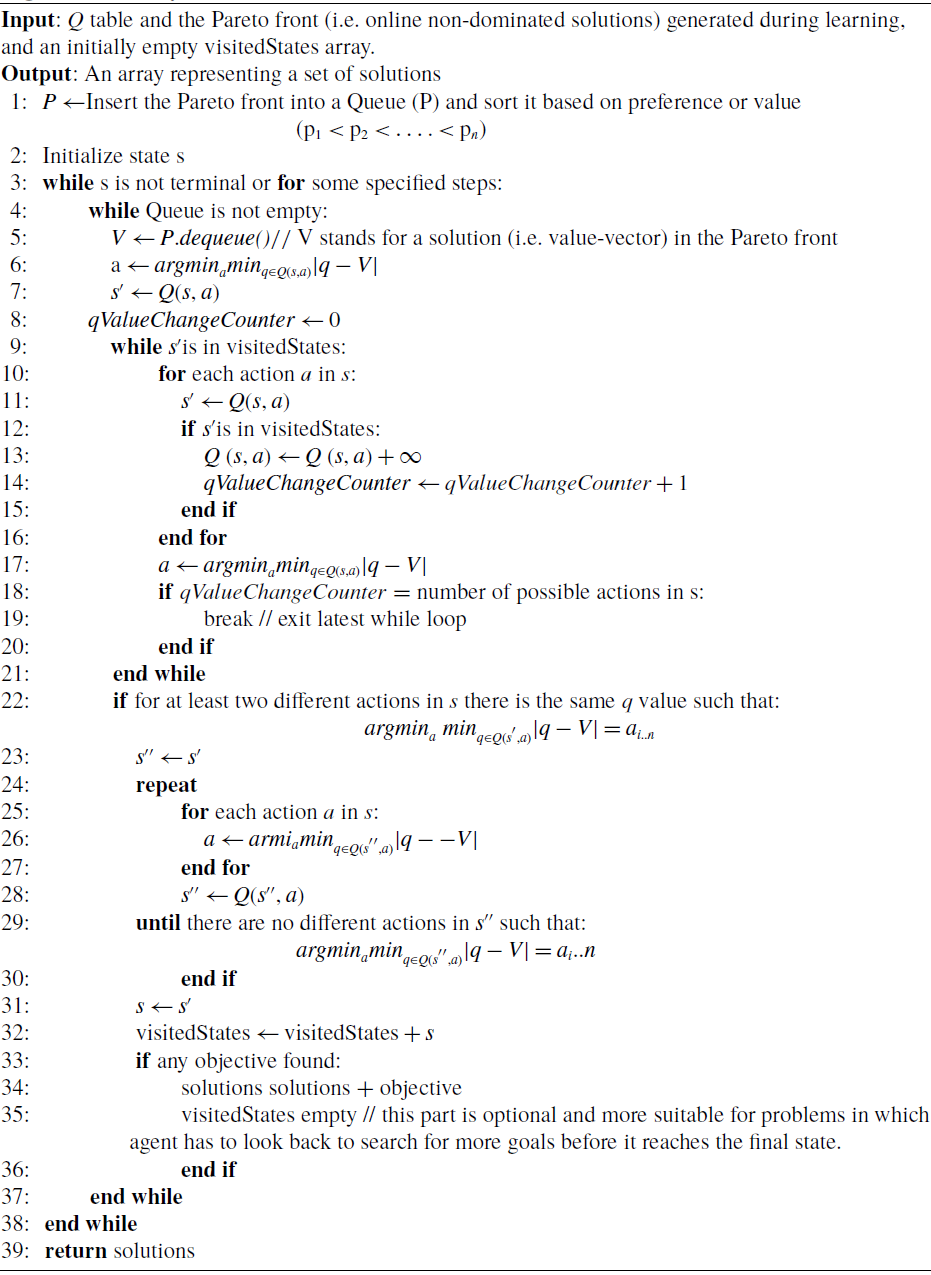
According to Moffaert and Nowé (Reference Moffaert and Nowé2014) and Roijers et al. (Reference Roijers, Röpke, Nowe and Radulescu2021), applying arg-max operator on all actions in current state is more suitable for single-objective reinforcement learning and for multi-objective learning we need to define an adapted version of greedy action selection. With inspiration of the initial part of Roijers et al. (Reference Roijers, Röpke, Nowe and Radulescu2021) which selects the action minimizing the Manhattan distance of minimum Q-value of current state and desired value vector (i.e. reward or solution vector), we developed a new algorithm to search for a policy in offline mode. As Algorithm 9 demonstrates the process, each time a value vector is extracted from queue of online generated Pareto front and after selecting next action according to above mentioned rule, agent sees potentially next state $s'$ . There are some extra operations to prevent agent to get stuck in the loop and make it to get converged. First we need to mark visited states and crossing off them from the list of states which agent will go to by assigning them a big Q-value. Lines 8 to 21 of Algorithm 9 do that. Also in research it was found that there may be some duplicate Q-values which causes agent to get stuck in the infinite loop or navigate it to a wrong direction. So lines 22 to 30 agent looks up the next states of states in which there are duplicate Q-values and continues to search if there are duplicate values in subsequent states. Finally agent goes to the next state. For some problems agent does not need to look back to gather rewards and needs to proceed in depth in search space so there is no need to gravitate toward those states which visited before, so visited states is marked for this kind of problems and line 35 which nullifies the respective array is not executed.

It is also challenging to evaluate multi-objective algorithms without using benchmark problems. Prior to the presentation of the benchmark problems, the researchers mentioned the results of problems in their papers that had nothing in common with each other and could not be compared. Also, since the Pareto Front is not specified for many problems, there is no basis for performance appraisal. Therefore, the existence of standard problems to evaluate the performance of algorithms and compare them with each other seems necessary (Vamplew et al., Reference Vamplew, Dazeley, Berry, Issabekov and Dekker2011). There are some instances of benchmark problems; here we mention two cases that the proposed model has been implemented to solve them.

Algorithm 9

Policy Search in Offline Mode

4.1 Deep sea treasure

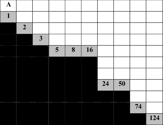
This problem and its environment, proposed by Vamplew et al. (Reference Vamplew, Dazeley, Berry, Issabekov and Dekker2011), is an episodic problem in which a submarine is looking for treasure in the deep sea. The problem has two objectives, one is to obtain more valuable treasures and the other is to minimize the time to collect those treasures. The environment of this problem is a gridworld consisting of 11 columns and 10 rows. As the distance from the initial state increases, the value of the treasures on the sea floor increases. The agent can move right, left, up, and down in this environment. With each move, the agent receives a reward vector with two members, one for the amount of treasure discovered and the other for the time. The reward for the treasure is zero where no treasure is discovered and is equal to the value of the treasure on steps where the treasure is found. The time with each move of the agent is considered as a penalty with a value of −1. The values of the other entries in the table are zero. Each episode either ends with the discovery of one of the treasures or after the agent has made the maximum allowed movement in each episode (maximum 1000 steps).

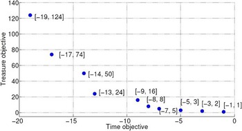
Figure 1 shows the problem environment: A represents the agent, black cells represent the seabed, and numbers in gray cells represent the value of the treasures. As Vamplew has suggested in Vamplew et al. (Reference Vamplew, Dazeley, Berry, Issabekov and Dekker2011), this problem is designed to illustrate the limitations of the scalarization methods. Figure 2 demonstrates the Pareto front of the problem and indicates that the front is globally concave.

Figure 1.

Deep sea treasure.

Figure 2.

Pareto front of deep sea treasure.

When assessing single-policy methods, they must be evaluated across a range of different weight settings. For the algorithms considered in this study, the weight for each objective lies in the range of 0 to 1, and their sum is equal to 1. So if we sample this weight space at a distance of 0.1, there are a total of 11 different sets of weight coefficients. In first version of proposed algorithm (Algorithm 9), according to (37) all 11 weight preferences are given to the algorithm as criteria together and simultaneously and there is no need for the user to specify them.

It should be noted that in linear and Chebyshev scalarization methods, the weights associated with each objective are set in the scalarization functions defined in (12) and (17) respectively:

(37) \begin{align*} {{\mathbf C}}_{{\mathbf 1}} [s,a]= MAX (0.0\quad {{\mathbf Q}}_{{\mathbf 1}} [s,a], 1.0\quad {{\mathbf Q}}_{{\mathbf 2}} [s,a])\nonumber\\[2pt]{{\mathbf C}}_{{\mathbf 2}} [s,a]= MAX (0.1\quad {{\mathbf Q}}_{{\mathbf 1}} [s,a], 0.9\quad {{\mathbf Q}}_{{\mathbf 2}} [s,a])\nonumber\\[2pt]{{\mathbf C}}_{{\mathbf 3}} [s,a]= MAX (0.2\quad {{\mathbf Q}}_{{\mathbf 1}} [s,a], 0.8\quad {{\mathbf Q}}_{{\mathbf 2}} [s,a])\nonumber\\[2pt]{{\mathbf C}}_{{\mathbf 4}} [s,a]= MAX (0.3\quad {{\mathbf Q}}_{{\mathbf 1}} [s,a], 0.7\quad {{\mathbf Q}}_{{\mathbf 2}} [s,a])\nonumber\\[2pt]{{\mathbf C}}_{{\mathbf 5}} [s,a]= MAX (0.4\quad {{\mathbf Q}}_{{\mathbf 1}} [s,a], 0.6\quad {{\mathbf Q}}_{{\mathbf 2}} [s,a])\nonumber\\[2pt]{{\mathbf C}}_{{\mathbf 6}} [s,a]= MAX (0.5\quad {{\mathbf Q}}_{{\mathbf 1}} [s,a], 0.5\quad {{\mathbf Q}}_{{\mathbf 2}} [s,a])\nonumber\\[2pt]{{\mathbf C}}_{{\mathbf 7}} [s,a]= MAX (0.6\quad {{\mathbf Q}}_{{\mathbf 1}} [s,a], 0.4\quad {{\mathbf Q}}_{{\mathbf 2}} [s,a])\nonumber\\[2pt]{{\mathbf C}}_{{\mathbf 8}} [s,a]= MAX (0.7\quad {{\mathbf Q}}_{{\mathbf 1}} [s,a], 0.3\quad {{\mathbf Q}}_{{\mathbf 2}} [s,a])\nonumber\nonumber\\[-35pt]{{\mathbf C}}_{{\mathbf 9}} [s,a]= MAX (0.8\quad {{\mathbf Q}}_{{\mathbf 1}} [s,a], 0.2\quad {{\mathbf Q}}_{{\mathbf 2}} [s,a])\nonumber\\[2pt]{{\mathbf C}}_{{\mathbf 10}}[s,a]= MAX (0.9\quad {{\mathbf Q}}_{{\mathbf 1}} [s,a], 0.1\quad {{\mathbf Q}}_{{\mathbf 2}} [s,a])\nonumber\\[2pt]{{\mathbf C}}_{{\mathbf 11}}[s,a]= MAX (1.0\quad {{\mathbf Q}}_{{\mathbf 1}} [s,a], 0.0\quad {{\mathbf Q}}_{{\mathbf 2}} [s,a])\end{align*}

In the second version of proposed algorithm (Algorithm 9), for example, if the user has a weight preference of 0.2 for the time and 0.8 for the treasure, Algorithm 8 forms two decision criteria for TOPSIS as follows:

(38) \begin{align} {{\mathbf C}}_{{\mathbf 1}} [s,a]= 0.2\quad {{\mathbf Q}}_{{\mathbf 1}} [s,a] \nonumber\\[3pt]{{\mathbf C}}_{{\mathbf 2}} [s,a]= 0.8\quad {{\mathbf Q}}_{{\mathbf 2}} [s,a]\end{align}

The two criteria $C_1$ and $C_2$ for each decision or action that the agent has to choose are thereby quantified, and as there are four actions in the DST environment, the 4 $\times$ 2 decision matrix is formed.

$Q1\ [s,\ a]$ is the value of Q table related to the time objective and associated state s and action a and $Q2\ [s,\ a]$ is the value of table Q related to the treasure objective and associated state s and action a.

In this section, we compare the performance of the TOPSIS Q-Learning algorithm with the Linear Scalarization and the Chebyshev algorithms in DST environment. It should be noted that changes in exploration rate, number of episodes and learning rate affect the results and the results may differ from what is stated in other publications. In other papers, such as Moffaert et al. (Reference Moffaert, Drugan and Nowé2013), the number of episodes was considered less, but the Pareto front did not appear in the output. Here, because we are interested in having a solution, we considered the number of episodes to be high. All three algorithms were implemented with learning parameters including number of episodes = 10 000, maximum time step per episode = 1000, learning rate $(\alpha) = 0.9$ , discount factor $(\gamma ) = 0.8$ . Exploration rate $(\epsilon)$ decays during learning meaning that the exploration rate at the beginning is 100% and it gradually decreases to zero by the end of the algorithm.

The three algorithms of Linear Scalarization, Chebyshev and TOPSIS Q-Learning were run 10 times for each of the 11 weight preferences, which is equal to 110 times. It is worth mentioning since all 11 weight preferences are injected to the first version of the TOPSIS algorithm at once and we don’t need to run algorithm for each combination of weights separately, it is significantly cost-effective. However we ran the first version of the TOPSIS as many times as other algorithms to have a fair comparison. In the first version of the TOPSIS algorithm, each weight preference uses other weights to support uncertainty and variation. The criteria for the first version of the algorithm are formed as (37) and for the second version they are like (38).

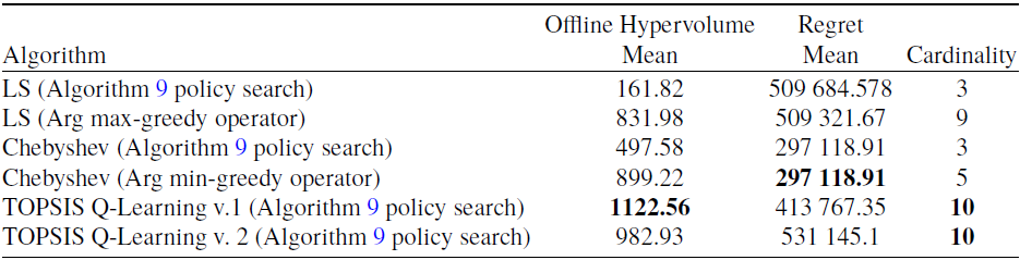
Then the hypervolume of offline rewards is calculated and averaged for the above specified number of experiments (i.e. runs). The hypervolume and also the regret mean is shown in Table 1. For the regret measure according to (35) after each episode, rewards are accumulated. Once the algorithm terminates, the accumulated reward is subtracted from the product of the total number of episodes and the optimal solution. Optimal solution is calculated as follows: first choose the maximum and minimum bounds for each objective either from true front or estimated from previous experiments, second create a hyperplane passing through the minimum and maximum bounds of the front, third calculate a point called $P_h$ on the hyperplane for a given set of preference weights and specify them as extrema of hyperplane, forth find the point $P_t$ on the Pareto front which minimizes | $P_h - P_t|$ (Vamplew et al., Reference Vamplew, Dazeley, Berry, Issabekov and Dekker2011).

Table 1.

Statistics of average performance of algorithms in DST environment

Table 2.

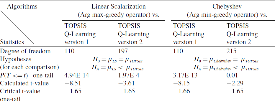
T-test for comparing LS and Chebyshev algorithms average offline hypervolumes with TOPSIS Q-Leaning algorithms in DST environment

In order to include all weights in the regret measure, the first version of the TOPSIS algorithm was run for all 11 weights so that all weights were taken into account in calculating the amount of the regret and especially the mean reward of each optimal solution defined in the regret formula.

Table 1 shows the average performance of the algorithms. Since LS and Chebyshev algorithms indicated poor hypervolume results with Algorithm 9 policy search, their greedy operators also have been included. It can be seen that both versions of the TOPSIS algorithms have higher values of hypervolume than the other two algorithms. But in terms of the regret measure Chebyshev algorithm outperformed the other two algorithms. In the case of cardinality both TOPSIS versions found maximum possible solutions in the Pareto front considering the total runs of the experiments.

In order to be able to infer the results of Table 1 statistically, we can use the t-test to compare the means of the hypervolumes and the regrets of the algorithms to see if there is a significant difference between them. The results of t-test related to comparisons of best hypervolume values of the Linear Scalarization and the Chebyshev algorithms (i.e. acquired by the greedy operators) with two versions of the TOPSIS Q-Learning algorithm are presented in Table 2. 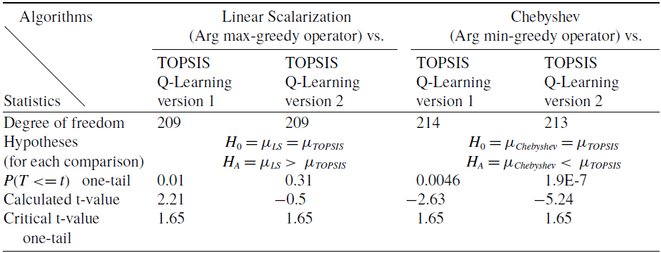As shown in Table 2 null hypothesis ( ${{\rm H}}_0$ ) is considered as the equality of means of the hypervolumes of the LS and the TOPSIS Q-Learning, and alterative hypothesis ( ${{\rm H}}_{{\rm A}}$ ) is the assumption of superiority or inferiority of TOPISIS Q-Learning algorithms against LS or Chebyshev algorithms and the same definition also applies to Table 3 and for the regret values. Our significance level is $\alpha =0.05$ and according to t-test procedure if p-value (p-value is the probability that the results obtained from our data occurred by chance) is less than $\alpha $ or absolute value of calculated t-value is greater than critical t-value, the null hypothesis is rejected and according to the alternative hypothesis, it can be statistically inferred that the mean of the hypervolume of the compared algorithms is significantly less than TOPSIS Q-Learning. The same principle applies to Table 3 for the regret measure. As it can be seen in Table 2 absolute values of all calculated t-values are greater than corresponding critical t-values and consequently all p-values are less than corresponding $\alpha = 0.05$ , so null hypothesis is rejected and we can infer that both versions of the TOPSIS Q-Learning algorithms performed significantly better than the other two algorithms in terms of the hypervolume mean. Table 3 demonstrates that since the absolute value of calculated t-value related to comparison of the Linear Scalarization and first version of TOPSIS algorithm is greater than its corresponding critical t-value and p-value of t-test is less than $\alpha= 0.05$ , null hypothesis is rejected and it can be inferred the average regret values of first version of the TOPSIS algorithm is significantly less than the Linear Scalarization algorithm. But about comparison of second version of the TOPSIS Q-Learning and the Linear Scalarization there is no significant difference between regret values of these algorithms considering lacking enough evidence to reject the null hypothesis. In the case of comparison of the Chebyshev algorithm with both versions of the TOPSIS Q-Learning, null hypothesis is rejected because as can be seen in the Table 3 absolute values of calculated t-values are greater than critical t-values and p-values are less than $\alpha = 0.05$ , so according to alternative hypothesis ( $H_A= {\mu }_{Chebyshev}<\ \ {\mu }_{TOPSIS\ }$ ) Chebyshev algorithm has much less regret values.

Table 3.

T-test for comparing LS and Chebyshev algorithms average regret with TOPSIS Q-Learning algorithms in DST environment

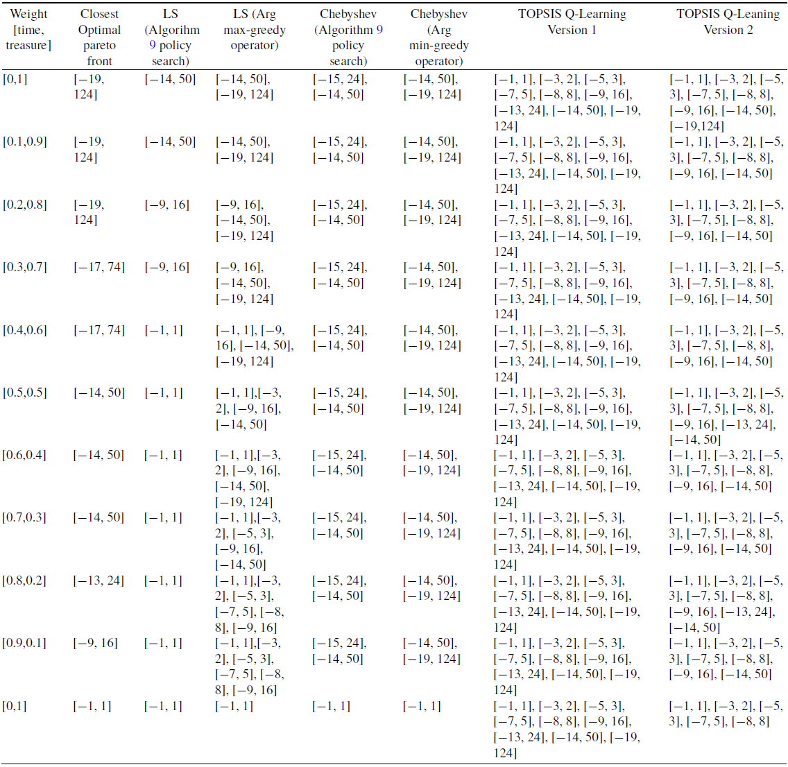
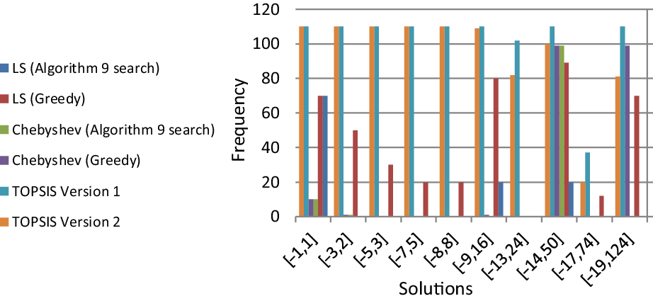
As mentioned before it is necessary for the agent to replicate the results achieved during learning in offline mode to ensure that the rewards are nonrandom and obtained policy is reliable. Even though in some runs of LS and TOPSIS algorithms more rewards have been acquired, in Table 4 offline results which occurred in every run of the algorithms have been presented and more details has been provided in Figure 3.

Table 4.

Offline results occurred in every run of all algorithms in DST environment

Figure 3.

Chart of frequency of all offline results discovered after learning process is finished in DST environment.

As it can be seen in Table 4 and Figure 3 LS algorithm could not find any desirable solution with Algorithm 9 policy search except for weight [0,1]. But with greedy operator it found all solutions except [−13, 24]. Solution with the value [−17, 74] is absent from Table 4 because it failed to be present in all runs of a specific weight. LS is able to find closest optimal Pareto front alongside other solutions at all weights except [0.3, 0.7], [0.4, 0.6], and [0.8, 0.2].The Chebyshev with Algorithm 9 search policy finds closest optimal policy only at weights [0.5, 0.5], [0.6, 04], [0.7, 03] and [0,1]. The Chebyshev with greedy policy could not find solution corresponding with weights [0.3, 07], [0.4, 0.6], [0.8, 0.2], [0.9, 0.1]. As it is observable in Figure 3 both Chebyshev experiments failed to generate different optimal results but [−14, 50] and [−19, 124]. The TOPSIS Q-Learning version 1 managed to find all optimal policies except for weights with values [0.3, 07] and [0.4, 0.6]. The algorithm also finds all other solutions except [−17, 74] alongside the closest optimal solution in every run of the experiments. Figure 3 demonstrates the TOPSIS Q-learning version 1 could find all optimal solutions during the experiments, although it found [−17, 74] less than the others because this reward did not occur in every run. The TOPSIS Q-Learning version 2 is unable to reach the optimal solution in every run at weights [0.1, 0.9], [0.2, 08], [0.3, 0.7], and [0.4, 0.6], as it can be seen in Figure 3 the algorithm found all solutions but [−17, 74] generated considerably less than the others. Looking at Figure 3 it can be said that in terms of spread among the solution space, the TOPSIS Q-learning version 1 has been more successful than the other algorithms as corresponding hypervolume value as a reflector of diversity in the Pareto front confirms this claim as well and all solutions but [−17, 74] are generated almost equally.

In order to ensure that the deepest treasure is found, the exploration parameter must be set to a high value number. In the experiment performed in Vamplew et al. (Reference Vamplew, Issabekov, Dazeley, Foale, Berry, Moore and Creighton2017), the exploration rate ( ${\rm{\varepsilon }} = 0.8$ ) or higher is used, which is decayed during learning. It should be mentioned these results are related to the TLQ algorithm, but the authors of the article observed similar results for the LS algorithm (Roijers et al., Reference Roijers, Zintgraf and Nowé2017). Therefore, if the exploration is not sufficient enough for the algorithm to find the most valuable treasure located in the convex area of the Pareto front, the algorithm will converge to one of the available solutions in the concave region. But it should be noted that the solutions located in the concave region are not really optimal, because the agent has not actually succeeded in finding the original optimal solution, which is located in a convex hull and is the most valuable. At the same time, the solution found is not entirely reliable, because the agent may reach the same solution in the concave region in a percentage of the tests, while ideally always converges to that truly optimal solution.

4.2 Resource gathering

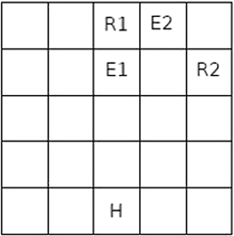
The environment of the problem as shown in Figure 4 is a table with 5 rows and 5 columns. The agent is in the home location and is allowed to move one of the four directions up, down, left, and right at any time. The resources that are gold and gem here are in specific places in the table, and the task of the agent is to collect one or both of the resources and return home. The agent receives a (+1) reward for each resource it returns home with.

Figure 4.

Resource gathering problem environment (Gabor et al., Reference Gabor, Kalmar and Szepesvari1998). H = home, R1 = gold resource, R2 = gem resource E1& E2 = enemy.

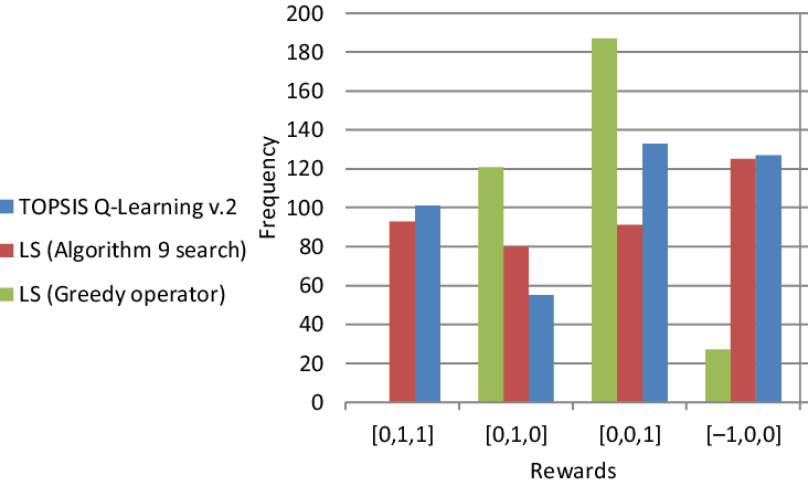
There are also two locations in the environment where the enemy may attack the agent with a 10% probability. In case of an attack, the agent loses a resource if it has any and is sent home with a penalty of −1. The reward vector is created as [attack, gold, gem] that there will be four possible states when returning to the home and a zero reward state [0, 0, 0] in other time steps (Gabor et al., Reference Gabor, Kalmar and Szepesvari1998):

• – [−1, 0, 0]: Agent being attacked

• – [0,0,1]: Return to the home with gold and without gem

• – [0,0,1]: Return to the home with gem and without gold

• – [0,1,1]: Return to the home with both gold and gem

This problem is mostly continuous and non-episodic in nature (Vamplew et al., Reference Vamplew, Dazeley, Berry, Issabekov and Dekker2011) but since all rewards are concentrated in the home location, its structure can be considered and implemented episodically.

Most of the researches discuss the total of rewards taken while learning and discovering the optimal policies to reach the resources. In the implementation of the algorithm, according to what was suggested in some papers, the total reward received during each episode is divided by the number of allowed steps in each episode (here the number of allowed steps is considered 100). Given that the number of possible combinations of weight preferences for the problem with 0.1 distances between them is 64, we are interested to use the TOPSIS Q-Learning version 2 to apply each specific weight preference of the entire objective space to the problem. For example if the preference of the first objective, that is, the probability of the enemy not attacking, is assumed to be 0.1 and the preference of the second and third objectives, that is, gold and gem to be equal to 0.1 and 0.8 respectively, criteria will be like as follows:

(39) $$\matrix{ {{{\bf{C}}_{\bf{1}}}[s,a] = {\rm{ }}\underline {0.1} \;{{\bf{Q}}_{\bf{1}}}[s,a]} \hfill \cr {{{\bf{C}}_{\bf{2}}}[s,a] = {\rm{ }}\underline {0.1} \;{{\bf{Q}}_{\bf{2}}}[s,a]} \hfill \cr {{{\bf{C}}_{\bf{3}}}[s,a] = {\rm{ }}\underline {0.8} \;{{\bf{Q}}_{\bf{3}}}[s,a]} \hfill \cr } $$

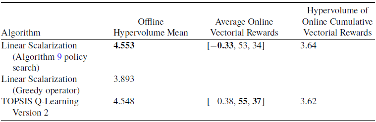
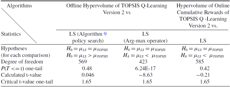
In this section, the TOPSIS Q-Learning algorithm is compared only with the LS algorithm and the comparison with the Chebyshev algorithm is omitted, because in Van Moffaert’s doctoral dissertation, a comparison was made between the Linear Scalarization and the Chebyshev algorithms and it has been observed that Linear Scalarization has been more successful in terms of obtaining the hypervolume as well as in terms of optimal policies (Moffaert, Reference Moffaert2014). According to a report in the same study, the Chebyshev algorithm was not able to discover a policy that could collect both gold and gem sources, while as we will see, both the TOPSIS and the Linear Scalarization algorithms (with Algorithm 9 policy search) are able to do that. Performance result of the TOPSIS Q-Learning algorithm is presented in Table 5. Different weight preferences are given to the second version of the TOPSIS Q-Learning algorithm as decision criteria analogous to relations defined in (39). The hypervolume measure whose reference point is [−2, −1, −1] was applied to final offline rewards to compare two algorithms performance. Also, because the use of the regret measure and determining the maximum and minimum bounds for each objective in a three-dimensional environment is more complex than the two-dimensional environment presented in the paper of Vamplew et al. (Reference Vamplew, Dazeley, Berry, Issabekov and Dekker2011) it was not used for the problem. Instead, the hypervolume was calculated for cumulative online reward vectors to assess algorithms online performance.

Table 5.

Average performance of algorithms in resource gathering problem

Table 6.

T-test for statistically comparing Linear Scalarization algorithm average offline and online hypervolume with TOPSIS Q-Leaning algorithm in DST environment

Both Algorithms were run 10 times for each weight preference set in which their elements sum equals to 1 and each weight element is greater than zero, so total number of runs would be 320. Both algorithms were run with the following learning parameters. Number of episodes = 100, maximum steps per episode = 100, learning rate ( $\alpha $ ) = 0.1, discount factor ( $\gamma $ ) = 0.95, exploration rate (ε) = 0.9. As demonstrated in the Figure 5, LS with greedy operator gained minimum penalty rewards, that is, [−1, 0, 0] and maximum gem reward but it could not obtain rewards containing both gold and gem. LS with Algorithm 9 policy search managed to discover [0,1,1] reward including gold and gem at the same time. The TOPSIS Q-Learning gained the most penalties and the least solo gold rewards. But it obtained maximum rewards of gems and dominated reward, that is, [0,1,1] compared to LS.

Figure 5.

Chart of frequency of offline rewards for TOPSIS Q-Learning and Linear Scalarization in resource gathering problem.

The hypervolume of offline rewards calculated after complete execution of the algorithms for above specified experiment repeat times is presented in Table 5. It can be seen here that unlike the DST environment, the LS algorithm performed better with Algorithm 9 policy search compared to using the greedy operator. The LS algorithm has a larger hypervolume with a small difference compared to the TOPSIS Q-Learning. So we should refer to t-test to see how significant this comparison is. The average vectorial rewards show that the TOPSIS Q-Learning algorithm has performed better than the Linear Scalarization in gaining gold and gem resources, although earning more rewards comes at a higher cost meaning receiving more penalties and gaining returns of [−1, 0, 0] during learning. However, to ensure that the relationship follows Pareto dominance, the hypervolume has been calculated in Table 5 and it shows LS has a slightly larger hypervolume. But considering p-value and calculated t-value, null hypothesis is not rejected and t-test proves this difference is not significant. So these algorithms are almost on the same level in terms of online performance.

The t-test was performed with the significance level ( $\alpha )$ of 0.05. According to the p-value of the LS implemented with Algorithm 9 policy search which is greater than $\alpha $ and absolute value of calculated t-value which is smaller than critical t-value, null hypothesis is not rejected and we can conclude that the TOPSIS Q-Learning and the LS have the close performance in terms of average offline hypervolume in resource gathering environment. The TOPSIS Q-learning outperformed the LS greedy version according to p-value and calculated t-value.

Declaration of competing interests

The authors declare that they have no known competing financial interests or personal relationships that could have appeared to influence the work reported in this paper.