2.1 DNS of temporal transition in channel flow

The three-dimensional incompressible Navier–Stokes (NS) equations with an external force are solved in a rectangular channel with sides $L_{x}=5.61$ , $L_{y}=2$ and $L_{z}=2.99$ in the streamwise $x$ -, the wall-normal $y$ - and the spanwise $z$ -directions, respectively. The velocity $\boldsymbol{u}=(u,v,w)$ is non-dimensionalized by the bulk velocity 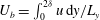$U_{b}=\int _{0}^{2\unicode[STIX]{x1D6FF}}u\,\text{d}y/L_{y}$ with the channel half-height $\unicode[STIX]{x1D6FF}=1$ . The time-dependent external force $\boldsymbol{f}(t)$ is equal to the wall-friction stress at each time step, so that the flow maintains a constant mass flux in the streamwise direction with $U_{b}\approx 1$ .

The NS equations are solved by the Fourier–Chebyshev pseudo-spectral method (Kim, Moin & Moser Reference Kim, Moin and Moser1987). Non-slip conditions are applied at the walls at $y=0$ and $y=2\unicode[STIX]{x1D6FF}$ , and periodic boundary conditions are applied in the streamwise and spanwise directions. A two-dimensional and a pair of three-dimensional Tollmien–Schlichting (TS) waves are imposed on the initial laminar Poiseuille flow to trigger the K-type transition. The streamwise wavenumber of all the TS waves is $k_{x}=2\unicode[STIX]{x03C0}/L_{x}=1.12$ , and the spanwise wavenumber of the three-dimensional waves is $k_{z}=2\unicode[STIX]{x03C0}/L_{z}=2.1$ . Thus, the computational domain contains one wavelength of the initial TS waves. We remark that the present computation domain is large enough to investigate the vortical structures in the late transition before reaching the fully developed turbulent state.

The numerical solver and initial disturbances used in the DNS have been described in detail in Zhao et al. (Reference Zhao, Xia, Shi, Xiao and Chen2014, Reference Zhao, Yang and Chen2016). After the flow reaches the fully developed turbulent state, the wall-friction Reynolds number $Re_{\unicode[STIX]{x1D70F}}=u_{\unicode[STIX]{x1D70F}}\unicode[STIX]{x1D6FF}/\unicode[STIX]{x1D708}=207.8$ is calculated, where $\unicode[STIX]{x1D708}$ is the kinetic viscosity and $u_{\unicode[STIX]{x1D70F}}=\sqrt{\unicode[STIX]{x1D70F}_{w}/\unicode[STIX]{x1D70C}}$ denotes the wall-friction velocity, with the wall shear stress $\unicode[STIX]{x1D70F}_{w}$ and the density $\unicode[STIX]{x1D70C}$ . The number of grids in all the directions are $N_{x}=384$ , $N_{y}=385$ and $N_{z}=384$ . The mesh sizes in wall units in the streamwise and spanwise directions are $\unicode[STIX]{x0394}x^{+}=3.04$ and $\unicode[STIX]{x0394}z^{+}=1.62$ , respectively, and the distance of the first grid point from the wall is $\unicode[STIX]{x0394}y_{w}^{+}=0.00695$ , which can obtain a highly resolved vorticity field. Here, the superscript ‘ $+$ ’ denotes a non-dimensional quantity scaled by the viscous length scale $\unicode[STIX]{x1D6FF}_{\unicode[STIX]{x1D708}}=\unicode[STIX]{x1D6FF}u/\unicode[STIX]{x1D708}$ .

2.2 VSF method for wall-bounded flow

The VSF $\unicode[STIX]{x1D719}_{v}$ is defined to satisfy the constraint $\unicode[STIX]{x1D74E}\boldsymbol{\cdot }\unicode[STIX]{x1D735}\unicode[STIX]{x1D719}_{v}=0$ , so that every isosurface of $\unicode[STIX]{x1D719}_{v}$ is a vortex surface consisting of vortex lines. The numerical methods for solving the VSF evolution equations are described in detail in Yang & Pullin (Reference Yang and Pullin2011). In the two-time approach, each time step is divided into prediction and correction steps. In the prediction step, the temporary VSF $\unicode[STIX]{x1D719}_{v}^{\ast }$ is evolved in physical time $t$ as a Lagrangian scalar as

where $\boldsymbol{u}$ is the velocity field from DNS. In general, the temporary $\unicode[STIX]{x1D719}_{v}^{\ast }$ deviates from an accurate VSF owing to the breakdown of the Helmholtz vorticity theorem in viscous flow. Then, in the correction step, $\unicode[STIX]{x1D719}_{v}^{\ast }$ is transported in pseudo-time $\unicode[STIX]{x1D70F}$ as

along the frozen vorticity field $\unicode[STIX]{x1D74E}$ at a fixed physical time to project the temporary VSF on the desired accurate VSF, with the initial condition $\unicode[STIX]{x1D719}_{v}(\boldsymbol{x},t;\unicode[STIX]{x1D70F}=0)=\unicode[STIX]{x1D719}_{v}^{\ast }(\boldsymbol{x},t)$ . Finally, $\unicode[STIX]{x1D719}_{v}^{\ast }$ in (2.1) is updated by $\unicode[STIX]{x1D719}_{v}(\boldsymbol{x},t;\unicode[STIX]{x1D70F}=T_{\unicode[STIX]{x1D70F}})$ from (2.2) for each physical time step, where $T_{\unicode[STIX]{x1D70F}}$ is a pseudo-time period that is typically less than 100 times the physical time step size.

The scalar equations (2.1) and (2.2) were advanced in $t$ and $\unicode[STIX]{x1D70F}$ , respectively, using the third-order total-variation-diminishing Runge–Kutta method and the convection terms were treated by the fifth-order weighted essentially non-oscillatory (WENO) scheme (Jiang & Shu Reference Jiang and Shu1996). The numerical diffusion in the WENO scheme can serve as a numerical dissipative regularization for (2.1) and (2.2).

Zhao et al. (Reference Zhao, Yang and Chen2016) suggested that the isosurface of the initial VSF $\unicode[STIX]{x1D719}_{v0}$ should be a stream surface other than a vortex surface in a transitional wall flow. Considering the plane Poiseuille flow or any other simple shear flow as $\boldsymbol{u}_{0}=(h(y),0,0)$ , the initial VSF should be set as $\unicode[STIX]{x1D719}_{v0}=f(y)$ , where $h(y)$ and $f(y)$ are arbitrary smooth functions of $y$ . The isosurfaces of such $\unicode[STIX]{x1D719}_{v0}$ are streamwise–spanwise planes and stay invariant in the laminar plane Poiseuille flow.

We propose the criteria to determine the wall-boundary conditions for the VSF equations (2.1) and (2.2). First, the isosurface of the VSF at the wall should be identical to the wall, so that the velocity and vorticity on the wall cannot change the VSF. Second, there should be no flux of the VSF through the wall to ensure that the scalar is conserved in the computation domain. Based on these criteria, the Neumann boundary condition is selected as $\unicode[STIX]{x2202}\unicode[STIX]{x1D719}_{v}/\unicode[STIX]{x2202}y|_{y=0,L_{y}}=0$ , where $y=0$ and $y=L_{y}$ are the wall locations of a channel flow. Then we can set the initial VSF as $\unicode[STIX]{x1D719}_{v0}=1-\cos (\unicode[STIX]{x03C0}y/L_{y})$ . Isosurfaces of $\unicode[STIX]{x1D719}_{v0}$ with $0\leqslant \unicode[STIX]{x1D719}_{v0}\leqslant 1$ represent the initial vortex surfaces from the bottom wall for $\unicode[STIX]{x1D719}_{v0}=0$ to the midplane at $y=L_{y}/2$ for $\unicode[STIX]{x1D719}_{v0}=1$ within the lower half the channel.

In general, the computed $\unicode[STIX]{x1D719}_{v}$ cannot be exact, and the deviation of isosurfaces of $\unicode[STIX]{x1D719}_{v}$ from vortex surfaces is quantified by the cosine of the angle between the vorticity $\unicode[STIX]{x1D74E}$ and the scalar gradient $\unicode[STIX]{x1D735}\unicode[STIX]{x1D719}_{v}$ as $\unicode[STIX]{x1D706}_{\unicode[STIX]{x1D714}}\equiv \unicode[STIX]{x1D74E}\boldsymbol{\cdot }\unicode[STIX]{x1D735}\unicode[STIX]{x1D719}_{v}/(|\unicode[STIX]{x1D74E}||\unicode[STIX]{x1D735}\unicode[STIX]{x1D719}_{v}|)$ (see Yang, Pullin & Bermejo-Moreno Reference Yang, Pullin and Bermejo-Moreno2010; Yang & Pullin Reference Yang and Pullin2011). The VSF scalar is calculated on the uniform grids $N_{x}^{v}\times N_{y}^{v}\times N_{z}^{v}=768\times 769\times 768$ , with $\boldsymbol{u}$ and $\unicode[STIX]{x1D74E}$ interpolated onto the grids for the VSF calculation. 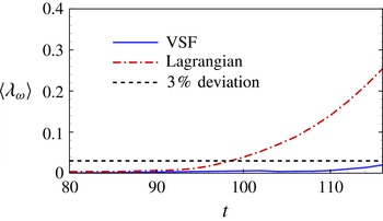The temporal evolution of the averaged deviation $\langle \unicode[STIX]{x1D706}_{\unicode[STIX]{x1D714}}\rangle$ is shown in figure 1, where $\langle \cdot \rangle$ denotes the volume average. The deviation in the evolution of the Lagrangian scalar field with the VSF initial condition in Zhao et al. (Reference Zhao, Yang and Chen2016) is also presented for comparison, which can be large during vortex reconnection owing to the violation of the Helmholtz theorem. In contrast, the deviation of the VSF calculation is below $3\,\%$ , which is much less than the Lagrangian result. Therefore, the present VSF calculation with the proposed wall-boundary conditions can provide a relatively accurate VSF in the transitional channel flow. Additionally, the accuracy of the VSF calculation can be further improved by increasing the grid resolution of the VSF with additional computation costs (Yang & Pullin Reference Yang and Pullin2011).

Figure 1.

Temporal evolution of $\langle \unicode[STIX]{x1D706}_{\unicode[STIX]{x1D714}}\rangle$ , where $\unicode[STIX]{x1D706}_{\unicode[STIX]{x1D714}}$ is the cosine of the angle between the vorticity $\unicode[STIX]{x1D74E}$ and the scalar gradient. Solid line: VSF scalar $\unicode[STIX]{x1D719}_{v}$ ; dash-dotted line: the Lagrangian scalar; dashed line: the 3 % level.

3.1 Visualization of vortex reconnection

We extract the isosurfaces of the VSF to study the evolution of vortex surfaces in the late stage of transition. In the earlier linear instability and weakly nonlinear instability stages (Herbert Reference Herbert1988; Kachanov Reference Kachanov1994) before $t=100$ , the initial disturbances gradually amplify, but no obvious vortical structure occurs before the strong nonlinear interactions of instability modes at around $t=85$ . 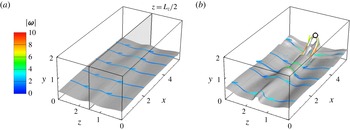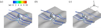Evolving from the initial vortex sheets parallel to the wall, the vortex surfaces display significant deformation from the late transition stage. Before vortex reconnection, the evolutionary geometry of the isosurface of $\unicode[STIX]{x1D719}_{v}=0.2$ in figure 2 is similar to that of the corresponding material surface in Zhao et al. (Reference Zhao, Yang and Chen2016). The vortex surface evolves through a triangular bulge at $t=100$ into a hairpin-like structure at $t=108$ , and a secondary hairpin-like structure begins to form at the upstream of the primary one. The tip of the triangular bulge and the head of the hairpin-like structure are located at the spanwise midplane, because the imposed TS waves and evolving vortical structures are symmetric with respect to the plane at $z=L_{z}/2$ (Klebanoff, Tidstrom & Sargent Reference Klebanoff, Tidstrom and Sargent1962).

Figure 2.

Temporal evolution of the isosurface of the VSF with $\unicode[STIX]{x1D719}_{v}=0.2$ , (a) $t=100$ ; (b) $t=108$ . Vortex lines are integrated from the surfaces, and colour-coded by the magnitude of vorticity $|\unicode[STIX]{x1D74E}|$ . The spanwise symmetric plane is shown by the translucent plane-cut at $z=L_{z}/2$ . The open circle indicates the position of $d_{min}$ .

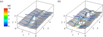
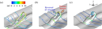
Since the significant vortex reconnection is expected to occur near the centre of the channel where two lifted vortical structures from opposite halves of the channel appear to collide (Zhao et al. Reference Zhao, Yang and Chen2016), the isosurface of $\unicode[STIX]{x1D719}_{v}=0.55$ remote from the wall is shown in figure 3. As the hairpin-like vortical structure from the lower half of the channel is lifted into the upper half, the vortex lines at its ‘head’ are surrounded by vortex lines with opposite directions pointing into or out the spanwise symmetric plane. In figure 3(a), the vortex lines reconnect with the opposite vortex lines at the position marked by the open circle at $t=110$ , and a pair of tube-like structures are attached to the hairpin-like structure. In figure 3(b), at a later time $t=114$ , the hairpin-like structure deforms remarkably, and the vorticity magnitude is significantly intensified near the reconnection position due to the stretching and twisting of vortex tubes. The large-scale, tube-like vortical structures can be further stretched and twisted into small-scale structures, resulting in the final transition to turbulence. This scenario of scale cascade is similar to the observation of the VSF evolution in the Taylor–Green flow (Yang & Pullin Reference Yang and Pullin2011).

Figure 3.

Temporal evolution of the isosurface of the VSF with $\unicode[STIX]{x1D719}_{v}=0.55$ , (a) $t=110$ ; (b) $t=114$ . Vortex lines are integrated from the surfaces, and colour-coded by $|\unicode[STIX]{x1D74E}|$ . The open circle indicates the reconnection position identified by $d_{min}\approx 0$ .

Figure 4.

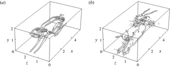
Isosurfaces of the swirling strength $\unicode[STIX]{x1D706}_{ci}$ with 20 % of the maximum value, (a)  $t=110$ ; (b) $t=114$ .

For comparison, the Eulerian vortical structures are extracted by the isosurfaces of the swirling strength $\unicode[STIX]{x1D706}_{ci}$ , which is the imaginary part of the complex eigenvalue of the velocity gradient tensor (Zhou et al. Reference Zhou, Adrian, Balachandar and Kendall1999). Although the cores of the hairpin-like structures in figure 4 are identified, the isosurfaces of $\unicode[STIX]{x1D706}_{ci}$ and other Eulerian-based vortex identification methods (not shown) cannot accurately characterize the reconnections at $t=110$ and $t=114$ as those identified by the VSF in figure 3. Compared with the reconnection of vortex surfaces or lines shown by the VSF, the visual ‘breakdown’ of the Eulerian vortical structures at $t=114$ is elusive in terms of the physics of scale cascade in fluids.

In order to further investigate the detailed process of the reconnection of vortex surfaces and lines, we zoom in the isosurfaces of the VSF at different time instants around $t=110$ in figure 5. At $t=109.6$ , the vortex line from the upper half channel is very close to the isosurface of the VSF with $\unicode[STIX]{x1D719}_{v}=0.55$ , but there is no topological change in vortex surfaces and lines. At $t=110$ , the vortex lines begin to reconnect near the location identified by the open circle in figure 5(b) on the spanwise symmetric plane, and the tube-like structures rolled up from the upper half are attached to the hairpin-like structure. At $t=110.4$ , the tube-like structures are stretched downwards, and then are rolled up and twisted into the structures shown in figure 3(b).

Figure 5.

Details of the isosurface of the VSF with $\unicode[STIX]{x1D719}_{v}=0.55$ , (a) $t=109.6$ ; (b) $t=110$ ; (c) $t=110.4$ . Vortex lines are integrated from the surfaces, and colour-coded by $|\unicode[STIX]{x1D74E}|$ . The open circle indicates the reconnection position identified by $d_{min}\approx 0$ .

Moreover, three different isosurfaces of the VSF at $t=110$ are shown in figure 6 to display the complex vortical structures during vortex reconnection. These isosurfaces beneath the isosurface of $\unicode[STIX]{x1D719}_{v}=0.55$ in figure 3 are close to the wall and show different topologies of the vortex surfaces initially at different wall distances. The isosurface of $\unicode[STIX]{x1D719}_{v}=0.25$ shows the core of the primary hairpin-like vortex with strong vorticity on the attached vortex lines. The isosurface of $\unicode[STIX]{x1D719}_{v}=0.37$ contains a reversed secondary $\unicode[STIX]{x03A9}$ -shaped structure with weak vorticity, which is lifted through two ‘legs’ of the primary hairpin by the induced velocity of the ‘legs’. The vortex lines on the reversed $\unicode[STIX]{x03A9}$ -shaped structure can reconnect at its ‘neck’ to form ring-like vortex lines near the head of the primary hairpin in figure 6(c), and they gradually vanish, perhaps owing to viscous dissipation.

Figure 6.

Different isosurfaces of the VSF at $t=110$ , (a) $\unicode[STIX]{x1D719}_{v}=0.25$ ; (b) $\unicode[STIX]{x1D719}_{v}=0.37$ ; (c) $\unicode[STIX]{x1D719}_{v}=0.4$ . Vortex lines are integrated from the surfaces, and colour-coded by $|\unicode[STIX]{x1D74E}|$ . The arrows indicate different directions of movement of the typical vortical structures.

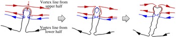
A schematic diagram of the process of vortex reconnection based on the typical vortex lines extracted from the VSF isosurfaces at $t=108$ , $t=110$ and $t=112$ is presented in figure 7. Two types of reconnection based on the viscous cancellation of vorticity vectors with opposite signs (Kida & Takaoka Reference Kida and Takaoka1994) are identified by the red and blue vortex lines, respectively. One is the reconnection of the red vortex lines at the ‘hairpin head’ and the relatively straight vortex lines from the opposite half of the channel. The lines are cut at the spanwise symmetric plane and then become two branches in the left and right halves of the channel. The other is the reconnection of the ‘legs’ of a $\unicode[STIX]{x03A9}$ -shaped vortex line. The blue line breaks at the ‘neck’ and generates a vortex ring and a long helical vortex line. Finally, the geometry of the vortex lines after reconnection can become very convoluted under their interactions and self-induced motions.

Figure 7.

A schematic diagram of the process of vortex reconnection. The skeleton of the evolving vortex surface is presented by typical vortex lines marked by different colours. The extracted vortex lines from left to right are attached on the VSF isosurfaces at $t=108$ , $t=110$ and $t=112$ , respectively. The reconnection events are marked by the dashed arrows.

3.2 Quantification of vortex reconnection

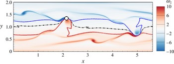
Based on the VSF evolution, we develop two quantitative methods to identify the incipient vortex reconnection. The first method is the separation distance between the vortical structures, which is natural to identify vortex reconnection. Hussain & Duraisamy (Reference Hussain and Duraisamy2011) defined the location of the vortex tubes as the centroid of the area where the vorticity magnitude is larger than a certain value. Nevertheless, the isosurface of vorticity magnitude or other Eulerian vortex identification methods are challenging to accurately characterize reconnection in shear flows as shown in figure 4.

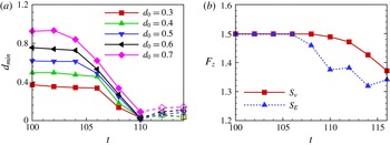
On the other hand, the isosurfaces of the VSF naturally provide the location of vortex surfaces. We use the minimum distance $d_{min}$ between a pair of vortex surfaces with $\unicode[STIX]{x1D719}_{v}=L_{y}/2\pm d_{0}$ to quantify the vortex reconnection of the evolving vortex surfaces from the opposite halves of the channel, where $d_{0}>0$ is a half of the distance between the wall-parallel vortex sheets at the initial laminar state. The temporal evolution of $d_{min}$ is shown in figure 8(a). The positions of $d_{min}$ on vortex surfaces are marked by the open circle in figures 2(b) and 3(a). In figure 8(a), $d_{min}$ decreases for all the vortex pairs due to the elevation of hairpin-like structures, and $d_{min}$ reaches the minimum at $t=110$ , which is defined as the reconnection time $t_{R}$ , which agrees with the visualizations in figures 2 and 3. In figure 9, the reconnection location with $d_{min}\approx 0$ is marked by the open circle, where different vortex surfaces converge. After the reconnection at $t_{R}\approx 110$ , $d_{min}$ is calculated from the new structures after topological changes rather than the original vortex surfaces, and it is presented by the dashed lines.

Figure 8.

Quantification of vortex reconnection, (a) the minimum distance $d_{min}$ between a pair of vortex surfaces $\unicode[STIX]{x1D719}_{v}=L_{y}/2\pm d_{0}$ ; (b) the vorticity flux $F_{z}$ through a certain region on the spanwise symmetric plane, where $S_{v}$ denotes the region between two vortex surfaces with $\unicode[STIX]{x1D719}_{v}=0$ and $\unicode[STIX]{x1D719}_{v}=L_{y}/2$ , and $S_{E}$ denotes the half-plane between $y=0$ and $y=L_{y}/2$ .

Figure 9.

Contour of the spanwise vorticity $\unicode[STIX]{x1D714}_{z}$ on the symmetric plane-cut at $z=L_{z}/2$ at $t=110$ . The black dash-dotted line shows the isoline of $\unicode[STIX]{x1D719}_{v}=L_{y}/2$ , and the red and blue solid lines represent the isolines of $\unicode[STIX]{x1D719}_{v}=L_{y}/2-0.45$ and $\unicode[STIX]{x1D719}_{v}=L_{y}/2+0.45$ , respectively. The open circle indicates the reconnection position identified by $d_{min}\approx 0$ .

Moreover, the evolution of the vorticity flux through a symmetric plane between a pair of reconnecting vortices can also quantify vortex reconnection (see Melander & Hussain Reference Melander and Hussain1989). We select the $x$ – $y$ plane-cut at $z=L_{z}/2$ as the symmetric plane, as presented in figure 2(a), and calculate the vorticity flux $F_{z}\equiv \int _{S}\unicode[STIX]{x1D714}_{y}\,\text{d}S$ through a certain region $S$ on the plane.

The temporal evolution of the vorticity flux $F_{z}$ is shown in figure 8(b). The red solid and blue dashed lines represent $F_{z}$ calculated through $S_{v}$ , the region enclosed by the bottom wall and the isoline of $\unicode[STIX]{x1D719}_{v}=L_{y}/2$ , and $S_{E}$ , the half-plane between $y=0$ and $y=L_{y}/2$ , respectively. According to the Helmholtz vorticity theorem, $F_{z}$ through $S_{v}$ , rather than $S_{E}$ , is conserved in inviscid flows. In figure 9, the dash-dotted isoline of $\unicode[STIX]{x1D719}_{v}=L_{y}/2$ can clearly divide the symmetric plane into two regions with opposite spanwise vorticity. Thus, $F_{z}$ calculated through $S_{v}$ is almost conserved before $t_{R}\approx 110$ in figure 8, and begins to decrease at $t_{R}\approx 110$ . This also indicates the incipient vortex reconnection at $t_{R}$ and the subsequent vortex reconnections after $t_{R}$ , because the viscous cancellation causing the separation of vortex lines at the spanwise symmetric plane can largely reduce $F_{z}$ , as illustrated in figure 7. On the other hand, $F_{z}$ calculated through the Eulerian half plane $S_{E}$ decreases earlier than the actual reconnection time, because the hairpin-like structures with negative $\unicode[STIX]{x1D714}_{z}$ lifted from the upper half can enter the region $S_{E}$ .

Therefore, the VSF facilitates the identification of the reconnection time via two different methods – $d_{min}$ and $F_{z}$ through $S_{v}$ . Both methods find that the incipient reconnection time is around $t=110$ in the present flow, which is consistent with the visualizations in § 3.1.

3.3 Vortex reconnection and the surge of wall friction

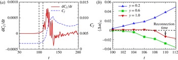
The temporal evolution of the wall-friction coefficient $C_{f}\equiv 2\unicode[STIX]{x1D70F}_{w}/(\unicode[STIX]{x1D70C}U_{b}^{2})$ and its temporal derivative $\text{d}C_{f}/\text{d}t$ is shown in figure 10(a), with the wall shear stress $\unicode[STIX]{x1D70F}_{w}\equiv \unicode[STIX]{x1D70C}\unicode[STIX]{x1D708}(\unicode[STIX]{x2202}\langle u\rangle _{xz}/\unicode[STIX]{x2202}y)|_{y=0}$ , where $\langle \cdot \rangle _{xz}$ denotes the average over the $x$ – $z$ plane. The increase of $C_{f}$ begins at $t=100$ with a relatively slow growth rate, and then it increases sharply after the identified reconnection time $t_{R}\approx 110$ .

Figure 10.

Vortex reconnection and the surge of wall friction, (a) temporal evolution of the wall-friction coefficient $C_{f}$ (dash-dotted line) and its temporal derivative $\text{d}C_{f}/\text{d}t$ (solid line); (b) temporal evolution of the averaged streamwise velocity change $\langle \unicode[STIX]{x0394}u\rangle _{xz}$ .

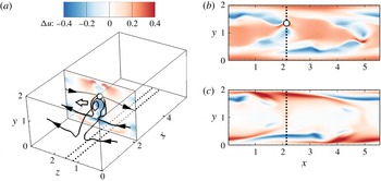
The increasing wall friction is mainly caused by the induced motion of vortical structures, as the ejection and sweep events in wall-bounded turbulent flows (Adrian Reference Adrian2007). The contours of the streamwise velocity change $\unicode[STIX]{x0394}u\equiv u-u_{0}$ are shown in figure 11(a), with the typical vortex lines and the induced velocity vector near the hairpin-like structure. Here, $u_{0}$ denotes the initial streamwise velocity in the initial laminar state. At the reconnection time $t_{R}\approx 110$ , the hairpin-like vortex lines and the vortex ring can induce a negative streamwise velocity from the Biot–Savart law, which behaves as a semipermeable membrane to partially block the flow near the centre of the channel. Subsequently, the near-wall streamwise velocity increases in general to maintain a constant mass flux with $U_{b}=1$ in figures 11(b) and11(c).

Figure 11.

Contours of the streamwise velocity change $\unicode[STIX]{x0394}u$ at $t=110$ . (a) Translucent contour on the $x$ – $z$ plane-cut at the reconnection position marked by the open circle. Typical vortex lines are shown by the black solid lines, the induced velocity near the ‘hairpin head’ is marked by the open arrow, and the positions of the $x$ – $y$ plane-cuts in (b) and (c) are marked by the black dotted lines; (b) contour on the spanwise symmetric plane at $z=L_{z}/2$ ; (c) contour on the plane-cut near the ‘hairpin leg’.

The temporal evolution of the averaged streamwise velocity change $\langle \unicode[STIX]{x0394}u\rangle _{xz}$ is presented in figure 10(b). At the late stage of transition, the induced motion of the vortical structures causes an increase of $\langle \unicode[STIX]{x0394}u\rangle _{xz}$ near the wall at $y=0.2$ and a decrease of $\langle \unicode[STIX]{x0394}u\rangle _{xz}$ remote from the wall at $y=0.6$ . It is interesting that $\langle \unicode[STIX]{x0394}u\rangle _{xz}$ at the midplane at $y=L_{y}/2$ hardly changes until $t_{R}\approx 110$ . During vortex reconnection, the geometric change of reconnecting vortex lines and the strong intensification of the vorticity magnitude, as shown in figures 3 and 11, significantly decelerate the fluids near the centre of the channel and indirectly cause a sudden increase of the wall friction in this incompressible, constant mass-flux channel flow.

Furthermore, the concurrence of vortex reconnection and the surge of wall friction is also validated in other transitional channel flows with different initial disturbances by varying the magnitudes and wavenumbers of the initially imposed TS waves. We observe similar vortex reconnection of the hairpin-like vortex lines and the vortex lines from the opposite half of the channel. The reconnection times are varied, but the sudden increases of wall friction consistently begin at the reconnection times in different flow cases.