Introduction

Ice surface temperature controls the rate of sea-ice growth, and thus is a critical parameter for sea-ice modeling and climate studies. Little effort has been directed to the retrieval of the sea ice surface temperature in the Arctic, an area where the first effects of a changing climate are expected to be seen. The reason is not one of methodology, but rather our limited knowledge of atmospheric temperature, humidity, and aerosol profiles, the microphysical properties of polar clouds and ice crystal fogs, and the spectral characteristics of the wide variety of surface types found there. Such applications require frequent sampling over large areas. NOAA Advanced Very High Resolution Radiometer (AVHRR) thermal imagery can provide ice-pack surface skin temperatures under clear-sky conditions in a manner similar to that used operationally to estimate sea-surface temperatures. When clouds are present, the AVHRR-derived temperatures represent a mixture of surface and cloud-top temperatures, depending on the cloud fraction and cloud optical depth. Brightness temperatures recorded by passive microwave sensors are a function of physical temperature at frequency-dependent depths in the snow/ice column and, in general, are much less affected by atmospheric water. Passive microwave data also supply information on ice concentration and a first-order estimate of the proportion of first-year and multi-year ice.

Snow/ice temperatures as estimated from both AVHRR and passive microwave data are functions primarily of physical temperature, emissivity, ice concentration, and ice thickness. Penetration depth in the snow/ice column increases as microwave frequency decreases. Thus, the microwave temperatures represent the physical temperature and emissivity at different depths in the ice pack (including snow on the ice surface), whereas the AVHRR-derived values represent surface or very-near-surface temperatures. The key variables in the temperature calculations are the emissivities of different surface types at the microwave frequencies, the mix of surface types in the sensors’ fields-of-view, and atmospheric effects at the AVHRR frequencies. By combining passive microwave data with AVHRR imagery, we increase the number of variables available to address the unknowns in the surface temperature problem.

Our objectives are to use physical surface temperatures derived from AVHRR imagery (T_s(AVHRR)) combined with Defense Meteorological Satellite Program (DMSP) Special Sensor Microwave/Imager (SSM/I) passive microwave data to convert AVHRR-derived surface temperature T_s(AVHRR) (which includes a mixture of temperatures of water and ice within the field-of-view) to ice surface temperature T_ice(AVHRR) ; and to use the resulting T_ice(AVHRR) to convert the passive microwave brightness temperatures T_B to physical, passive microwave-derived surface temperature T_ice(PM) (or, at specific frequencies, T_ice(19V), T_ice(37V), T_ice(85H) ). In addition, since T_s(AVHRR) may actually represent both surface and atmospheric temperatures depending on cloud cover, while the SSM/I data at 19 and 37 GHz are considerably less affected by atmospheric conditions, we investigate whether the combination of T_ice(AVHRR) and T_ice(PM) can be used as a crude discriminator of cloud cover.

Data

AVHRR data were extracted from an image set prepared by the Naval Research Laboratory (Reference Fetterer and HawkinsFetterer and Hawkins, 1991). These data consist of AVHRR Local Area Coverage imagery calibrated and mapped to a polar stereographic grid of nominal 1 km cell size co-registered to the DMSP SSM/I brightness temperature grid format used to archive SSM/I data (NSIDC, 1990). The images are visually screened to minimize cloudy images in the archive, but no cloud masking is performed. Images for 1 March, 17 March, 23 March, 1 December and 2 December 1989 covering portions of the Beaufort Sea were extracted and converted to T_s(AVHRR) using the procedure described below. Each AVHRR image was resampled to a grid cell size of 25 km to match the SSM/I grid.

Concurrent SSM/I 19 GHz vertically polarized (19V), 37 GHz vertically polarized (37V), and 85 GHz horizontally polarized (85H) brightness temperatures were extracted from the daily gridded SSM/I images archived on CD-ROM (NSIDC, 1990). Total ice concentration and multiyear ice percentages were calculated using a version of the NASA Team Algorithm (Reference Gloersen and CavalieriGloersen and Cavalieri, 1986) and tie points supplied by NSIDC with the CD-ROMs. The 85H data (originally 12.5 km × 12.5 km) and the ice concentration output (50 km × 50 km) were resampled to match the 25 km cell size of the 19V and 37V grids. These gridded data consist of averaged samples for all orbits during a 24 h period, whereas the AVHRR data used are for individual orbits. Thus, some error in combining the SSM/I and AVHRR data is introduced due to the time-averaging involved.

Methodology

Physical temperature retrieval from AVHRR

The general approach to estimating surface temperature is to relate satellite observations to surface-temperature observations with a regression model. Lacking sufficient observations however, satellite radiances or brightness temperatures can be modeled by application of the radiative-transfer equation. This “forward model” approach is commonly used for retrieval of sea surface temperature. A means to correct for the atmospheric attenuation of satellite-measured clear sky brightness temperatures in the split-window thermal channels of the AVHRR sensors on-board three of the NOAA series satellites has been developed and is detailed in Reference Key and HaefligerKey and Haefliger (1992). These corrections are specified for three different “seasons” (summer, winter, and transition between winter and summer) and as a function of satellite viewing angle, and are expected to be applicable to the perennial ice pack in the central Arctic Basin. In this analysis it is assumed that a valid cloud-clearing method exists and that only clear sky radiances are being examined. The cloud-clearing problem in polar satellite data is not trivial, however. For a review of polar cloud detection algorithms, see Reference Key and BarryKey and Barry (1989) and Reference Sakellariou, Leighton and LiSakellariou and others (1992).

For the retrieval of the snow/ice surface temperature a multi-channel algorithm that uses empirical relationships to correct for water vapor absorption is employed:

(1)

where T₄ and T₅ are the satellite-measured brightness temperature (K) in the AVHRR thermal channels and θ is the sensor scan angle. The coefficients are determined through a least-squares regression procedure, where surface temperatures are regressed against modeled brightness temperatures. To model radiances in the AVHRR thermal channels, daily temperature and humidity profiles collected by rawinsonde from a Soviet ice island (NP-26), located at approximately 85° N, 170° W during 1983–87 are used to describe atmospheric conditions in each season for input to the LOWTRAN 7 radiative transfer model (Reference KneizysKneizys and others, 1988). Radiances are modeled for sensor scan angles from 0° to 60° in 10° increments. The appropriate sensor response function is applied to the calculated radiances, and radiances are then converted to brightness temperatures. Atmospheric chemical composition, background tropospheric and stratospheric aerosols for the subarctic winter and summer models are used, since no such information is available from the ice islands. The optical properties of Arctic haze have not been extensively measured; model calculations (Reference Blanchet and ListBlanchet and List, 1983) show that the volume extinction coefficient of Arctic haze is generally of the same order of magnitude as that of the tropospheric aerosols. Therefore, the use of tropospheric background aerosols is appropriate.

Concerning surface characterization, directional surface emissivities for snow are modeled as in Reference Dozier and WarrenDozier and Warren (1982). These emissivities are then integrated with the sensor response function for each channel. The skin temperature for each temperature profile is assigned a series of values during the month to which the profile belongs. An energy balance model (Reference MaykutMaykut, 1982) is used to determine these surface temperatures, based on the observed range of shelter temperatures and wind speeds (the mean ± 1 standard deviation) in the ice island data for each month. Overall, the accuracy of the estimated surface temperatures is approximately 0.1 K (Key and Haefliger, 1992). This value will be slightly larger in practice, since the sensor noise and model bias have not been taken into account.

As noted earlier, the AVHRR temperatures represent the integrated temperatures of all the surfaces within the field-of-view. Over pack ice, the resulting surface temperature can thus be a mixture of the surface temperatures of thick ice, thin ice and open water. Since we are primarily interested in the surface temperatures of the ice itself, we can combine T_s(AVHRR) and the SSM/I-derived ice concentrations to determine T_ice(AVHRR), where:

(2)

T_water the physical temperature of open water, is taken to be a salinity-adjusted 271.2 K. C_tot is the total ice concentration estimated from the SSM/I data. This approach ignores the effects of thin ice, but should be valid as a first approximation. At the thermal wavelengths considered here, we assume emissivities to be unity for both ice and water. For typical mid-winter ice concentrations and temperatures, a 5% error in C_tot yields an error in T_ice(AVHRR) of about 1 K.

Passive microwave-derived temperatures and emissivities

Since T_ice(AVHRR) is a skin or very-near-surface temperature, emissivities affecting T_ice(AVHRR) are not the same as the emissivities affecting the passive microwave T_B, due to the penetration depth at the passive microwave frequencies. We can consider our calculated emissivities as “effective” emissivities, ε′, that yield the appropriate skin temperature relative to the passive microwave T_B.

To calculate the physical temperature at the radiating layer from passive microwave data, we expand on the approach described by Reference Cavalieri, Gloersen and CampbellCavalieri and others (1984):

(3)

where f represents a particular frequency and polarization, ε is the radiating-layer emissivity, C is ice concentration, T_B is brightness temperature, fy represents first-year ice, and my represents multi-year ice. T_PM is the temperature of the radiating layer whereas T_ice(AVHRR) (and T_ice(PM) derived later) is a skin temperature. By including the different ice types, we can estimate T_PM at finer spatial resolution by using higher frequencies (compared to T_PM estimated using lower frequencies, since spatial resolution increases as frequency increases) where the variation in emissivity between first-year and multi-year ice is significant. The limitations of this simple method are that the emissivities and concentrations of the different ice types and open water must be provided. Since the NASA Team Algorithm operates essentially independently of physical temperature (Cavalieri and others, 1984) the derived concentrations are valid for our purpose. The largest sources of error lie in the emissivities and in the algorithm-derived multi-year ice concentration. A per cent error in emissivities translates into an equivalent per cent error in T_ice(PM). We therefore need to consider how to estimate the emissivities and how to minimize the error due to uncertainties in the C_my.

Since at microwave frequencies, ε = T_B/T_PM, we can estimate an “effective” emissivity, ε′, using T_B and T_ice(AVHRR), bearing in mind that T_ice(AVHRR) represents clear-sky surface temperatures. The relationship between the passive microwave-derived skin temperature, T_ice(PM), the effective emissivity and the brightness temperature T_B is now T_ice(PM) = Τ_B/ε′. However, ε′ differs for first-year and multi-year ice, with the difference being greatest at higher frequencies. If we choose only areas that have ice concentrations close to 100% and accept the NASA Team Algorithm’s output, we can reduce the equation to two unknowns, that can be solved as a set of simultaneous equations given multiple observations. We selected T_s(AVHRR) for a relatively clear-sky region in the 1 December AVHRR temperature image and used the corresponding ice concentration image to select only those pixels with C_tot greater than or equal to 99%. Based on these samples and solving Equation (4) yields the emissivities in Table 1. We reiterate that the estimate of multi-year ice concentration from the NASA Team Algorithm (e.g. the tie points used to represent the different ice types) defines the relationship between effective emissivity and ice type mixture. Thus, if T_ice(AVHRR) is available, the calculation of surface temperature from the SSM/I data is independent of the actual emissivity of the ice.

(4)

Table 1.

Effective emissivities, ε′, estimated using T_ice(AVHRR), SSM/I-derived concentrations, and Equation (4)

Fig. 1.

“Effective” emissivity at 19V, 37V and 85H versus multi-year ice concentration, for total ice concentrations of 99–100%. Emissivities are derived from AVHRR ice surface temperatures relative to the multi-year ice percentage estimated using the NASA Team Algorithm.

The high values for ε′ at 19V likely reflect the greater penetration depth at this frequency, since temperatures deeper in the ice or at the snow/ice interface are likely to be higher than the skin temperatures, given the typical winter conditions of heat conduction from the ocean upward through the ice column. As expected, the difference in emissivity between ice types increases with frequency due to volume scattering. Since we know that one of the largest sources of error in our approach is the potential error in the estimated multi-year ice percentage, the effect of this error on the ice temperature retrievals can be minimized by using the 19 GHz data.

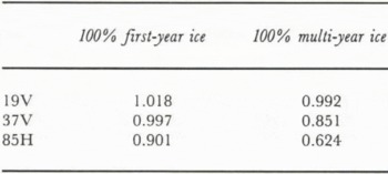
Using data from a region that appears to be relatively cloud-free in the 1 December image, we illustrate the frequency relationship between emissivity and multi-year ice percentage for near-100% ice cover more clearly in Figure 1. In addition to showing the change in emissivity with frequency, this plot suggests a second approach to calculate ε′ — simply fitting a line through each frequency’s data. The resulting equations are shown on the figure. Using these relationships, we arrive at the set of ε′ listed in Table 2. Both sets of ε′ are similar. Subsequent calculations of T_ice(PM) (e.g., T_ice(19V), T_ice(37V), and T_ice(85H) ) from the SSM/I data use the emissivities in Table 1.

Table 2.

Effective emissivities for 100% first-year ice and 100% multi-year ice estimating using a linear fit of ε′ vs multi-year ice percentage

Results

T_ice(AVHRR) and T_ice(19V) for 1 December and 2 December are shown in Figure 2. T_ice(AVHRR) shows greater spatial variability, with some patterns suggestive of cloud cover, whereas T_ice(19V) show an overall smoother transition of temperatures. In general, the microwave-derived temperatures are lower than the AVHRR temperatures, with the difference increasing as ice temperature decreases. Since lower ice temperatures are typically associated with a greater percentage of multi-year ice, this difference may be due to an overestimate of multi-year ice emissivity. The difference may also be due to thin cloud cover or ice fog that is hard to detect by eye in the AVHRR imagery. In a few locations, just north of Point Barrow in the southern Beaufort Sea for example, T_ice(19V) is higher than T_ice(AVHRR) suggesting that these are regions of high, cold cloud. Alternatively, these locations may have been closer to true “clear sky” conditions than the locations used to select clear-sky tie points, resulting in estimated effective emissivities that are too low. T_ice(37V) are nearly identical to T_ice(19V), while T_ice(85H) show much more variability, due most likely to a combination of greater sensitivity to surface scattering and to atmospheric emissions. Since 85H has the shallowest penetration depth of the SSM/I frequencies, some of the variation may also reflect spatial variations in skin temperature, as opposed to the temperatures sensed at 19 and 37 GHz which, due to the greater penetration depths at these frequencies, will have a dampened spatial and temporal response compared to skin temperatures.

Fig. 2.

Temperatures derived from AVHRR data for 1 December 1989 (a), 2 December 1989 (b). Surface temperatures derived from SSM/I 19V for 1 December 1989 (c) and 2 December 1989 (d). The area shown is a polar stereographic projection covering the western Arctic. Isotherm intervals are K. Land is masked out as black in the AVHRR and the SSM/I data, and the missing data zone around the pole is masked out as cross-hatching in the SSM/I data. Locations of sample transects (transects A and B) are shown by the heavy dashed lines labeled “A” and “B” in Figure 2c.

National Meteorological Center monthly mean surface air temperatures tend to be about 240 Κ north of about 77° in December and 235–240 K in March (Reference Parkinson, Comiso, Zwally, Cavalieri, Gloersen and CampbellParkinson and others, 1987) in the western Arctic. A summary of Soviet drifting station data from the Canada Basin show mean air temperatures of 242 Κ in March and 244 Κ in December while drifting buoy temperatures are typically about 5 Κ higher (Maslanik, unpublished data). Given the fact that radiative cooling of the ice surface will yield lower skin temperatures compared to air temperatures, the remotely-sensed surface temperatures are not unreasonable. A more direct comparison of T_ice(19V), T_ice(37V) and T_ice(AVHRR) is shown in the transect plots in Figures 3 and 4 for the December and March images. The microwave-derived temperatures show virtually no change along the transect from 1 December to 2 December, while considerable change is apparent in T_ice(AVHRR), again most likely due to changes in cloud cover and atmospheric water content, and possibly to surface warming due to enhanced downwelling longwave radiation beneath the cloud cover. T_ice(19V) and T_ice(37V) show a realistic decrease northward and toward the Canadian Archipelago, with the same general pattern along part of the T_ice(AVHRR) transect. The pattern of T_ice(AVHRR) in the northern portions of the grids — particularly the spatial pattern and the day-to-day changes such as the 14 Κ decrease at transect location 75 from 1 December to 2 December — suggest that the positive temperature bias between T_ice(AVHRR) and T_ice(19V) and T_ice(37V) may be due to cloud cover rather than differences in surface temperatures as estimated using the different imagery. However, we have no independent and reliable cloud information available to verify this. Differences in T_ice(19V) and T_ice(AVHRR) for 1 March, 17 March and 23 March are shown in Figure 4. The change in T_ice(19V) over time in the south suggest a possible decrease in surface air temperature over time, with little change further northward, while T_ice(AVHRR) shows a greater variability consistent with transient cloud cover. It is also possible that the radiating temperature of the ice pack itself might be changing over time due to ridging or snowfall. To examine further the differences between the AVHRR and passive microwave-derived temperatures and the relationship to cloud cover, we compare the image of T_ice(AVHRR) (Fig. 5a) and the image resulting from T_ice(AVHRR) − T_ice(19V) (Fig. 5b) for 1 December 1989. Figure 5a and b show spatial patterns typical of cloud cover. In Figure 5b, T_ice(AVHRR) is typically greater than T_ice(19V) by an average of about 2 Κ in the areas that have the appearance of cloud.

Fig. 3.

Comparison of T_ice(AVHRR) (— line), T_ice(19V) (– · – line), and T_ice(37V) (– … – line) for 1 December 1989 (a) and 2 December 1989 (b) along transect A in Figure 2.

Fig. 4.

Temperatures along transect Β in Figure 2 for 1 March, 17 March and 23 March 1989. Solid line is T_ice(19V), dashed line is T_ice(AVHRR). Dates for each transect are shown (e.g. “1” = 1 March, etc.).

The fact that some cloud might be delineated in this way does not, however, imply that having T_ice(PM) provides a general solution to the polar cloud detection problem. The accuracy of threshold-based cloud retrievals (e.g. all pixels that have temperatures above/below the surface temperature plus some ofTset) using T_ice(PM) depends on the error in T_ice(PM) and the temperature difference and sign of the difference between clouds and the surface. This case study presents a method for deriving T_ice(PM), but considerably more work is needed to estimate the accuracy of the method. Regarding the cloud and surface temperature relationships, in the December data examined here, apparent cloud cover (based on manual interpretation of spatial patterns in the AVHRR temperatures) has a broad temperature range, both colder and warmer than the surface. The amount of cloud that would go undetected using a simple thresholding procedure depends obviously on the temperature differential between cloud and surface, and on the error margin of T_ice(PM). Additionally, warm surface features such as leads and polynas may be falsely labeled as cloud. It is also important to point out that the relationship between the radiating temperature within the snowpack versus the skin temperature is complex, and few data exist to test the stability over time and space of the “clear-sky” tie points used here.

The problems noted above do not imply that passive microwave-derived surface temperatures are not useful for cloud detection algorithms. On the contrary, determining the surface temperature is the crucial step in the procedure. However, it is also clear that in the polar regions, having the surface temperature alone is generally not enough to map cloud cover, and that temporal and possibly textural characteristics must also be examined (see, for example, Key and Barry, 1989 and references therein).

Fig. 5.

Image of AVHRR temperatures (a) and the image resulting from T_ice(AVHRR) minus T_ice(19V) (b). Examples of apparent clouds (based on manual interpretation of T_ice(AVHRR) are labeled. The temperature range in (b) is about 35 K. Geographic area shown is the same as that in Figure 2.

Conclusions

We demonstrate how AVHRR and passive microwave imagery can be used to: (1) adjust AVHRR- derived temperatures to yield ice-only temperatures; (2) “calibrate” the passive microwave data to permit the calculation of ice pack temperatures from the microwave brightness temperatures; and (3) provide an additional tool for cloud mapping during winter. The most direct uses for microwave-derived temperatures may be in ice modeling, as a way to validate energy-balance calculations of snow/ice interface temperatures and surface temperatures, and also as a tool to refine passive microwave classifications of ice type. We have no means to determine absolute accuracy of the remotely sensed temperatures derived here, although comparison to climatological data suggest that the temperatures are reasonable. A more precise comparison is planned using single-orbit SSM/I data combined with buoy and ice station observations, and with data collected during the 1992 Seasonal Sea Ice Monitoring and Modelling Site (SIMMS) field program.

Acknowledgements

This work was supported by NASA grants NAGW-2158 and NAGW-2407 (University of Washington subcontract No. 721566). We thank Florence Fetterer and Jeff Hawkins for providing the AVHRR imagery, the National Snow and Ice Data Center for the SSM/I data, and Micaela Reddy for drafting assistance.