


Impact Statement
The Arctic is undergoing substantial transformation due to climate change, with consequences that are already visible at local and global scales. Melt ponds, which are puddles of water that form on summer sea ice, play an important role in regulating the Arctic’s energy balance. Accurately representing melt ponds alongside sea ice and open water in observations is essential to improve climate model parameterizations. This research advances the availability of melt pond observations and segmentation algorithms, supporting more accurate monitoring of Arctic sea ice conditions and contributing to a deeper understanding of the processes driving Arctic climate change.
1. Introduction
The Arctic region is warming at a rate three to four times faster than the global average (Stocker, Reference Stocker2014; Rantanen et al., Reference Rantanen, Karpechko, Lipponen, Nordling, Hyvarinen, Ruosteenoja, Vihma and Laaksonen2022). Since the beginning of satellite observations about 50 years ago, Arctic sea ice extent has declined by about 12.7% per decade during the summer months (Meier and Stroeve, Reference Meier and Stroeve2022), and projections indicate that the Arctic Ocean may become seasonally ice-free before the middle of this century (Notz and Stroeve, Reference Notz and Stroeve2018). These transformations have profound local impacts on communities and ecosystems (Hovelsrud et al., Reference Hovelsrud, Poppel, Van Oort and Reist2011; Saros et al., Reference Saros, Anderson, Juggins, McGowan, Yde, Telling, Bullard, Yallop, Heathcote, Burpee, Fowler, Barry, Northington, Osburn, Pla-Rabes, Mernild, Whiteford, Andrews, Kerby and Post2019; Luo et al., Reference Luo, Luo, Dai, Xiao, Simmonds, Hanna, Overland, Shi, Chen, Yao, Duan, Liu, Zhang, Xu, Diao, Jiang and Gong2024) and may further influence weather variability in the mid-latitudes (Francis and Vavrus, Reference Francis and Vavrus2015; Cohen et al., Reference Cohen, Zhang, Francis, Jung, Kwok, Overland, Ballinger, Bhatt, Chen, Coumou, Feldstein, Gu, Handorf, Henderson, Ionita, Kretschmer, Laliberte, Lee, Linderholm, Maslowski, Peings, Pfeiffer, Rigor, Semmler, Stroeve, Taylor, Vavrus, Vihma, Wang, Wendisch, Wu and Yoon2020). Despite their importance, there are significant knowledge gaps about the polar regions, primarily due to missing observations and limited process understanding (Meredith et al., Reference Meredith, Sommerkorn, Cassotta, Derksen, Ekaykin, Hollowed, Kofinas, Mackintosh, Melbourne-Thomas, Muelbert, Ottersen, Pritchard, EAG, Pörtner, Roberts, Masson-Delmotte, Zhai, Tignor, Poloczanska, Mintenbeck, Alegría, Nicolai, Okem, Petzold, Rama and Weyer2019; Li et al., Reference Li, Guo, Cheng, Song, Ran, Feng, Che, Li, Wang, Duan, Shangguan, Chen, Jin, Deng, Su and Cao2025). One major uncertainty arises from the insufficient representation of small-scale surface processes, such as melt ponds, in larger-scale climate assessments.
1.1. Melt ponds on Arctic sea ice
Melt ponds are puddles of water that form on sea ice when temperatures exceed the freezing point of water during the summer months, causing the snow on the sea ice to melt and meltwater to accumulate in sea ice depressions. They are primarily observed on Arctic sea ice and rarely form in the Antarctic (Andreas and Ackley, Reference Andreas and Ackley1982). Melt ponds play a critical role in the Arctic energy balance. Due to their optical properties, they absorb significantly more sunlight than the white sea ice and snow (Fetterer and Untersteiner, Reference Fetterer and Untersteiner1998; Perovich et al., Reference Perovich, Grenfell, Light and Hobbs2002a; Grenfell and Perovich, Reference Grenfell and Perovich2004; Nicolaus et al., Reference Nicolaus, Gerland, Hudson, Hanson, Haapala and Perovich2010). This leads to an acceleration of the melting process of ice beneath ponds, which is estimated to be two to three times faster than that of bare ice (Fetterer and Untersteiner, Reference Fetterer and Untersteiner1998). A phenomenon called ice-albedo feedback (Curry et al., Reference Curry, Schramm and Ebert1995). This also means that the initial formation of melt ponds is accompanied by a rapid increase in their size, which can range from square centimeters to square kilometers (Perovich et al., Reference Perovich, Tucker and Ligett2002b). The extent of melt ponds is then mainly limited by the sea ice surface topography. On deformed sea ice with high surface roughness, melt pond coverage is limited to the “valleys” (typical coverage of 20 to 30% and approximately 60% maximum coverage), whereas on very smooth sea ice like landfast ice, large surface fractions (almost 80%) can be covered by melt ponds (Landy et al., Reference Landy, Ehn and ShieldsMand Barber2014). Melt ponds also increase the light transmittance from the surface to the ocean, with implications for the under-ice ecosystem (Light et al., Reference Light, Grenfell and Perovich2008; Nicolaus et al., Reference Nicolaus, Katlein, Maslanik and Hendricks2012; Katlein et al., Reference Katlein, Arndt, Belter, Castellani and Nicolaus2019).
Despite their important contribution to the sea ice-albedo feedback, surface heat budget, and mass balance of sea ice, most existing studies rely on large-scale datasets that primarily distinguish between sea ice and open water, leading to substantial uncertainties in model projections (Flocco et al., Reference Flocco, Schroeder, Feltham and Hunke2012; Hunke et al., Reference Hunke, Hebert and Lecomte2013). Addressing these gaps requires high-resolution observations that enable the parameterization of melt ponds alongside the sea ice and open water classes (Zhang et al., Reference Zhang, Schweiger, Webster, Light, Steele, Ashjian, Campbell and Spitz2018; Diamond et al., Reference Diamond, Schroeder, Sime, Ridley and Feltham2024).
1.2. Earth observation of melt ponds
1.2.1. Observation systems
Melt ponds can be observed using different means. Numerous studies are based on in-situ measurements, which offer high-precision data and serve as a foundation for understanding various underlying processes (e.g., Eicken et al., Reference Eicken, Grenfell, Perovich, Richter-Menge and Frey2004; Polashenski et al., Reference Polashenski, Perovich and Courville2012; Landy et al., Reference Landy, Ehn and ShieldsMand Barber2014). However, the remoteness of the Arctic Ocean makes these measurements rare and limited to small, localized regions.
Satellite-based observations are the only method that can cover the entire Arctic region on a regular basis, but the resolution of space-based melt pond retrievals is often compromised. For example, Moderate Resolution Imaging Spectrometer (MODIS), which provides daily complete coverage of the Arctic region, is constrained by a spatial resolution of 250 m–1 km (e.g., Tschudi et al., Reference Tschudi, Maslanik and Perovich2008; Rösel and Kaleschke, Reference Rösel and Kaleschke2011). This presents a challenge in accurately acquiring data at the individual pond level. Higher-resolution satellite imagery, such as that provided by Sentinel-2 (10 m spatial resolution, 6–7 day revisit time), has been employed in some studies (e.g., Niehaus et al., Reference Niehaus, Spreen, Birnbaum, Istomina, Jäkel, Linhardt, Neckel, Fuchs, Nicolaus, Sperzel, Tao, Webster and Wright2023). However, because of limitations in the acquisition area and duty cycle per orbit, such higher-resolution data do not cover the entire Arctic. Furthermore, all satellite observations in the visible and infrared domain are hampered by clouds, which cause large gaps in the observations.
Aerial imagery, obtained from aircraft such as planes, helicopters, or unmanned aerial vehicles (UAVs), often serves as an intermediary between local in-situ measurements and broad satellite observations. Airborne measurements enable the acquisition of regional information over areas up to several hundred square kilometers. They have the advantage of flexibility, as they can be targeted to specific areas of interest, and cloud cover can be avoided by flying below the clouds. Moreover, they can be utilized as a means of validating satellite retrievals, given that higher spatial resolution can often be attained and multiple sensors can be operated in parallel (e.g., Istomina et al., Reference Istomina, Heygster, Huntemann, Schwarz, Birnbaum, Scharien, Polashenski, Perovich, Zege, Malinka, Prikhach and Katsev2015; Wang et al., Reference Wang, Su, Landy, Leppäranta and Guan2020; Niehaus et al., Reference Niehaus, Spreen, Birnbaum, Istomina, Jäkel, Linhardt, Neckel, Fuchs, Nicolaus, Sperzel, Tao, Webster and Wright2023).
1.2.2. Thermal infrared radiometry
Previous methods that use aircraft or satellites to acquire melt pond data mainly rely on observations within the visible electromagnetic spectrum, that is, mainly photographs in RGB format (e.g., Perovich et al., Reference Perovich, Tucker and Ligett2002b; Lu et al., Reference Lu, Li, Cheng, Lei and Zhang2010; Wright and Polashenski, Reference Wright and Polashenski2018). These optical images are valuable because they capture surface structures in three spectral channels, where such features are especially distinguishable. However, the quality of the images depends on the time of day and the prevailing sunlight conditions. The presence of shadows, variable illumination, and extensive cloud cover (which is typical of the Arctic region) present challenges in the retrieval of melt ponds from optical imagery.
Here, we will extend the modality available for melt pond detection utilizing thermal infrared (TIR) imagery. Thermal infrared radiometers are instruments that measure the thermal radiation emitted from the Earth’s surface. This radiation can be translated into surface temperature (Thielke et al., Reference Thielke, Huntemann, Hendricks, Jutila, Ricker and Spreen2022). TIR measurements are less contingent on light conditions, thereby enabling data retrieval when the sun is low on the horizon. Furthermore, TIR is capable of identifying the locations of former melt ponds during the winter months when they are frozen and obscured by snow (Thielke et al., Reference Thielke, Fuchs, Spreen, Tremblay, Birnbaum, Huntemann, Hutter, Itkin, Jutila and Webster2023).
To date, there has been no investigation into the potential of TIR images for the detection of melt ponds. As infrared cameras can be readily deployed during helicopter campaigns, we expect that TIR in conjunction with optical sensors will be a viable method to supplement data in low-light conditions. Samples of these data are displayed in Figure 1.
Melt ponds, sea ice, and open water captured at two locations by two different sensors. For each location, images from both sensors were acquired simultaneously (in the same second). Top row: Thermal infrared (TIR) imagery, where brighter colors indicate warmer surface temperatures. Bottom row: Corresponding optical images shown for visual reference. The TIR images reveal the temperature variability among surface types that complicates classical segmentation approaches. In the top-left TIR image, melt ponds and open water appear brighter (warmer) than the darker sea ice, whereas in the top-right image, some melt ponds appear brighter and others darker (colder) than the surrounding ice. Location: Fram Strait region. Date: 18 July 2022 (AWI PS131/02, Kanzow, Reference Kanzow, Bornemann and Sawadkuhi2023).

Figure 1. Long description
The top row contains two TIR images where brightness indicates surface temperature. The top-left panel, at latitude 81.6093 and longitude 7.7926, shows dark sea ice floes with bright, warm melt ponds and open water channels. The top-right panel, at latitude 81.2958 and longitude 7.6167, shows a different thermal signature where some melt ponds are bright while others are darker than the surrounding grey ice.
The bottom row contains two corresponding VIS images for visual reference. The bottom-left panel shows large, fractured light-grey ice floes separated by black open water, with numerous small, dark-greenish melt ponds scattered across the ice surfaces. The bottom-right panel shows a similar scene of fragmented ice floes and melt ponds, providing a high-contrast optical baseline for the thermal data above.
1.3. Semantic segmentation of surface types
To quantify melt ponds from image acquisitions, the images must be divided into different surface classes. This is achieved through semantic segmentation, where each pixel is assigned a label that identifies its surface type. Existing approaches for melt pond detection can be broadly classified into two categories: (1) pixel-based and (2) object-based segmentation.
Pixel-based methods assume that the reflectance values across multiple spectral bands are indicative of the class of a given pixel. Many approaches using optical imagery are based on thresholding, where specific value ranges are set within each band to classify pixels into different surface types (e.g., Tschudi et al., Reference Tschudi, Curry and Maslanik2001; Perovich et al., Reference Perovich, Tucker and Ligett2002b; Inoue et al., Reference Inoue, Curry and Maslanik2008; Lu et al., Reference Lu, Li, Cheng, Lei and Zhang2010; Krumpen et al., Reference Krumpen, Haas, Hendricks, Hölemann, Kalmbach and Gerdes2011; Huang et al., Reference Huang, Lu, Lei, Xie and Li2016; Niehaus et al., Reference Niehaus, Spreen, Birnbaum, Istomina, Jäkel, Linhardt, Neckel, Fuchs, Nicolaus, Sperzel, Tao, Webster and Wright2023). Other approaches have employed supervised machine learning techniques, such as random forests, to classify optical data at the pixel level (e.g., Fuchs, Reference Fuchs2023b).
In contrast, object-based segmentation seeks to group multiple pixels into meaningful objects. For instance, Miao et al. (Reference Miao, Xie, Ackley, Perovich and Ke2015) and Wright & Polashenski (Reference Wright and Polashenski2018) initially applied edge detection and watershed operators to delineate segments. Subsequently, these segments were classified using a random forest classifier based on manually defined spectral, spatial, and texture features.
A requirement for these pixel- and object-based methods is that every single pixel can be assigned to one specific class. For object-based methods, an object like a melt pond has to consist of several pixels to leverage the spatial information. These conditions are not met for satellite data of lower resolution (
$ >100 $
 m), such as MODIS on Aqua and Terra satellites, or OLCI on Sentinel-3 satellites, where individual ponds can be smaller than the resolution of a pixel. Here, physical (Istomina et al., Reference Istomina, Heygster, Huntemann, Schwarz, Birnbaum, Scharien, Polashenski, Perovich, Zege, Malinka, Prikhach and Katsev2015) or machine learning methods (Rösel and Kaleschke, Reference Rösel and Kaleschke2011) have to be applied to the measured spectrum to retrieve melt pond fraction (MPF) per pixel. As the dataset introduced in this study has a resolution of 1 m and can therefore fully resolve melt ponds larger than one square meter, such approaches are not discussed further here.
The aforementioned methods are not applicable to TIR images for the following reasons:
-
• Temperature variability: The surface temperature of different surface types is subject to considerable temporal and spatial fluctuations in the Arctic summer. As the salinity of the ocean lowers its freezing point to around $ -1.8 $
 °C (de Vernal, Reference de Vernal and Gornitz2009), sea ice can sometimes be warmer or colder than the surrounding open water when temperatures are close to freezing in the summer. This variability makes it difficult to use pixel-based approaches for segmenting TIR measurements (Figure 1, top row).
-
• Low contrast: In TIR, the delineation of melt ponds suffers from low-gradient edges and blurred boundaries, which can result from haze, small temperature differences, and smooth temperature transitions between surface types (Figure 1, top right). This challenges object-based approaches that are sensitive to noise.

1.4. Deep learning for semantic segmentation
In the past few years, deep learning models have been increasingly applied to semantic segmentation through the use of neural networks that automatically extract high-level features from images. These features subsequently inform the classification process.
A wide range of model architectures are based on convolutional neural networks (CNNs) that slide learnable filters across the image dimensions to aggregate local information. Long et al. (Reference Long, Shelhamer and Darrell2015) leveraged CNNs for image segmentation with variable input sizes by introducing fully convolutional networks (FCNs), which employ convolutional and upsampling layers after feature extraction to predict a dense image output. Popular advancements of the FCN model include U-Net (Ronneberger et al., Reference Ronneberger, Fischer, Brox, Navab, Hornegger, Wells and Frangi2015) and UNet++ (Zhou et al., Reference Zhou, Rahman Siddiquee, Tajbakhsh, Liang, Stoyanov, Taylor, Carneiro, Syeda-Mahmood, Martel, Maier-Hein, Tavares, Bradley, Papa, Belagiannis, Nascimento, Lu, Conjeti, Moradi, Greenspan and Madabhushi2018), which use skip connections to improve pixel positioning. Zhao et al. (Reference Zhao, Shi, Qi, Wang and Jia2017) employed pyramid pooling for multi-scale feature extraction with the pyramid scene parsing network (PSPNet). Further, DeepLabV3+ (Chen et al., Reference Chen, Zhu, Papandreou, Schroff, Adam, Ferrari, Hebert, Sminchisescu and Weiss2018) combines pyramid pooling with an encoder-decoder structure to produce refined segmentation maps from context-rich representations.
More recently, transformer-based methods are used for semantic segmentation. Transformer-based models rely on attention mechanisms that model the dependencies between different image regions, aimed at capturing more global image context. Prominent examples include Vision Transformer (ViT)-based architectures that process images as a sequence of smaller patches (Dosovitskiy et al., Reference Dosovitskiy, Beyer, Kolesnikov, Weissenborn, Zhai, Unterthiner, Dehghani, Minderer, Heigold, Gelly, Uszkoreit and Houlsby2020; Strudel et al., Reference Strudel, Garcia, Laptev and Schmid2021; Xie et al., Reference Xie, Wang, Yu, Anandkumar, Alvarez and Luo2021). Kirillov et al. (Reference Kirillov, Mintun, Ravi, Mao, Rolland, Gustafson, Xiao, Whitehead, Berg, Lo, Dollár and Girshick2023) introduced Segment Anything (SAM) as the first foundation model for image segmentation. Its efficacy has been shown across a range of tasks, including remote sensing (Osco et al., Reference Osco, Wu, de Lemos, Gonçalves, Ramos, Li and Junior2023).
A limitation of deep learning models is that their performance relies on large amounts of training data, which requires labor-intensive manual labeling. This challenge has motivated various approaches to reduce labeling demands, such as semi-supervised learning, which uses both labeled and unlabeled data for training. For instance, Dynamic Mutual Training (DMT) has proven to be highly effective for segmentation tasks (Feng et al., Reference Feng, Zhou, Gu, Tan, Cheng, Lu, Shi and Ma2022; Peláez-Vegas et al., Reference Peláez-Vegas, Mesejo and Luengo2023). DMT is a pseudo-labeling method based on mutual learning, in which model disagreement is used to identify low-quality pseudo-labels. Another common strategy to address limited data is to pre-train the network’s feature extractor on a large dataset and then fine-tune the model on a smaller downstream dataset in a second step. This is often achieved by using pre-training datasets of natural images, for example, ImageNet (Deng et al., Reference Deng, Dong, Socher, Li, Li and Li2009), which provides a considerable amount of labeled data. In remote sensing, such extensive pre-training datasets remain scarce (Yuan et al., Reference Yuan, Shi and Gu2021). However, there are significant differences between these image domains. ImageNet contains RGB images of natural objects, including dogs and cars, taken from scenic viewpoints. In contrast, remote sensing images are captured from an overhead perspective across a range of geographical locations and spectral bands. This poses challenges for knowledge transfer (Rolf et al., Reference Rolf, Klemmer, Robinson and Kerner2024). Despite these differences, some research indicates that pre-training on ImageNet can still benefit downstream tasks in remote sensing (Hu et al., Reference Hu, Xia, Hu and Zhang2015; de Lima and Marfurt, Reference de Lima and Marfurt2019).
The objective of this paper is to present a new dataset of airborne TIR images and a method for the segmentation of these images into distinct surface types. During summer, the surface of the Arctic Ocean consists of three main surface types: melt ponds, sea ice, and open water (Wright and Polashenski, Reference Wright and Polashenski2018; Wright et al., Reference Wright, Polashenski, McMichael and Beyer2020). These classes have the strongest influence on surface albedo and thus play a key role in governing the surface energy balance of the Arctic Ocean. The resulting segmentation maps allow the derivation of geophysical parameters of primary scientific interest such as fractional surface coverage, melt pond size, and floe size distribution. The main contributions of this paper are as follows:
-
• For the first time, a TIR dataset acquired from a helicopter is provided for surface class segmentation into melt ponds, sea ice, and open water. Alongside this dataset, we make available 21 hand-labeled surface class annotations.
-
• We fine-tuned several segmentation architectures, including U-Net, UNet++, PSPNet, DeepLabV3+, and SwinTransformer, as well as two SAM-based networks, on this data. We also test pre-training weights from different natural image and remote sensing datasets.
-
• We test alternative loss functions and class balancing strategies that adjust the precision/recall trade-off of the predictions and enable user-specific fine-tuning.
-
• We evaluate the generalizability of individual predictions and out-of-distribution flights conducted over thin clouds and landfast ice.
-
• We apply the best-performing segmentation model to classify TIR images from multiple helicopter flights and present the resulting regional surface fractions.
Section 2 presents the data, while Section 3 introduces the methodology in more detail. The results are presented in Section 4 and discussed in Section 5.
2. Data
2.1. Study area and inventory
The dataset presented in this study consists of helicopter-borne TIR imagery captured by a VarioCAM HD head 680 camera produced by InfraTec. This camera records broadband infrared radiation within the 7.5 to 14
$ \mu $
 m range (Thielke et al., Reference Thielke, Huntemann, Hendricks, Jutila, Ricker and Spreen2022). The data were collected as part of the research icebreaker Polarstern PS131 ATWAICE campaign (Kanzow, Reference Kanzow, Bornemann and Sawadkuhi2023), which covered the marginal ice zone of the Fram Strait region (Figure 2). The campaign took place in July and August of 2022, when melt pond coverage is at its peak (Perovich et al., Reference Perovich, Tucker and Ligett2002b; Niehaus et al., Reference Niehaus, Spreen, Istomina and Nicolaus2025). A total of 16 helicopter flights were conducted at an altitude of approximately 300 m. The images were preprocessed following Thielke et al. (Reference Thielke, Huntemann, Hendricks, Jutila, Ricker and Spreen2022), including image gradient and drift correction. The resulting dataset contains images with a spatial resolution of about 1 m and a temporal resolution of one second, resulting in datasets containing 1000 to 6000 images with overlap for each flight.
Geographic location of the data collection in the Fram Strait region between Greenland and Svalbard (upper part of map). The red line marks the track of expedition PS131. Image source: Kanzow (Reference Kanzow, Bornemann and Sawadkuhi2023).
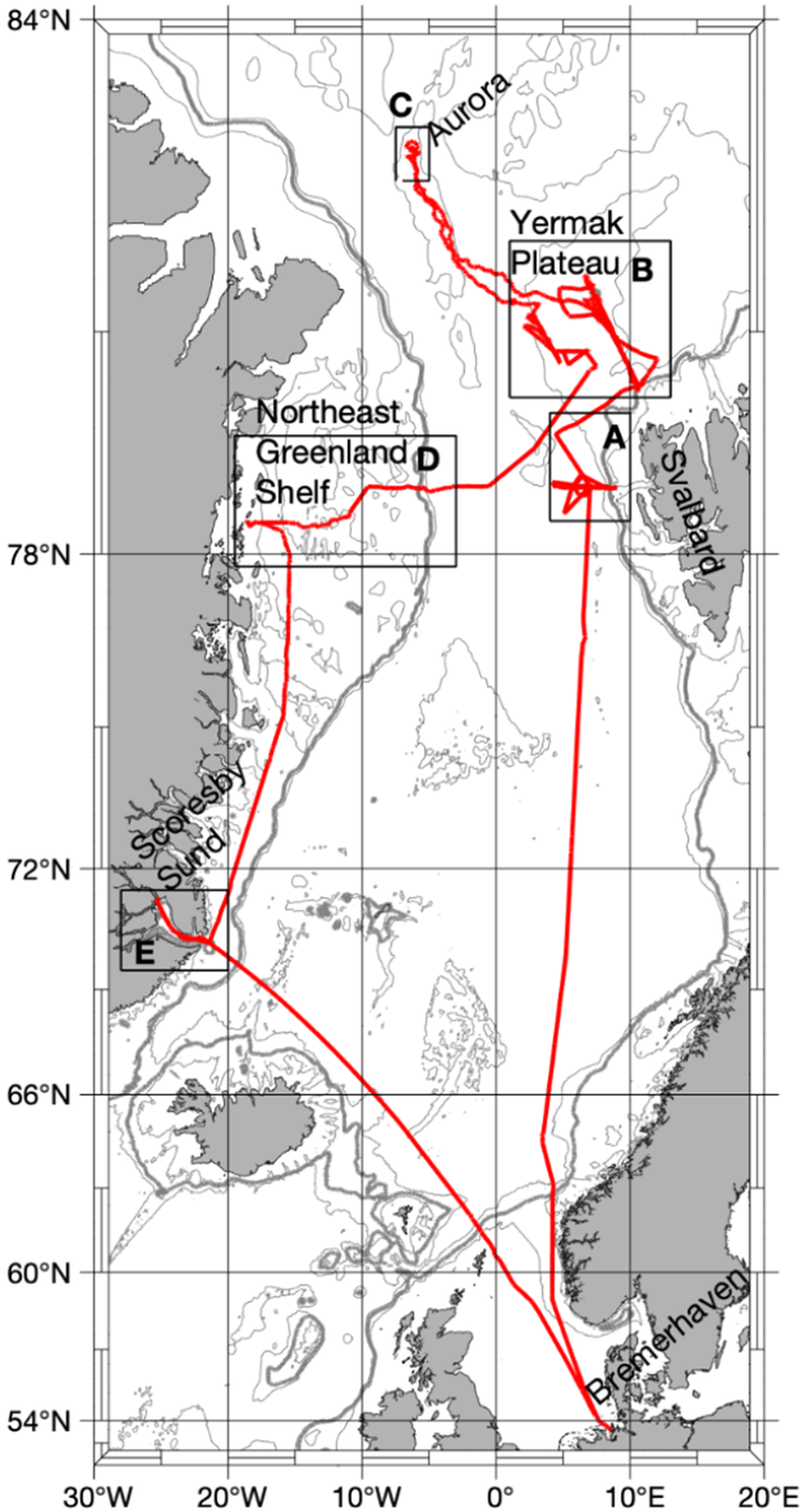
Figure 2. Long description
A geographical map with a latitude range from 54 degrees North to 84 degrees North and a longitude range from 30 degrees West to 20 degrees East. A solid red line represents the track of expedition PS131.
Starting in the South at Bremerhaven, Germany, the track moves North through the Norwegian Sea. At approximately 78 degrees North, the track enters the Fram Strait region between Greenland to the West and Svalbard to the East.
Five specific study areas are marked with black rectangular boxes and letter labels.
• Area A is located West of Svalbard.
• Area B is located North of Area A on the Yermak Plateau.
• Area C is the northernmost point of the track, labeled Aurora, located near 83 degrees North.
• Area D is located to the West on the Northeast Greenland Shelf.
• Area E is located further South along the Greenland coast at Scoresby Sund.
The track forms a large loop connecting these points, with a long transit line returning South-Southeast from Scoresby Sund back toward the European mainland.
Data is stored in NetCDF4 file format, with each image comprising
$ 640\times 480 $
 pixels and a single temperature channel. We also converted brightness temperature to surface temperature by dividing by a constant emissivity of 0.996. The data is made publicly accessible via the Pangaea data center (Reil et al., Reference Reil, Huntemann and Spreen2024).
2.2. Dataset creation for training and evaluation
To generate datasets for training and performance evaluation, we manually annotated 21 images from flight 7 (17 July 2022), 9 (18 July 2022), 10 (19 July 2022), 11 (19 July 2022), and 16 (30 July 2022) (see Table 3.4.2 in Kanzow, Reference Kanzow, Bornemann and Sawadkuhi2023). We excluded the remaining flights from labeling due to quality issues and ambiguities for the human annotator. The problems were caused by clouds or water vapor between the helicopter-mounted sensor and the surface, or artifacts caused by the EM-bird instrument, which was towed beneath the helicopter for several flights and appeared within the sensor’s field of view. While in principle, lower-quality flights could be included in the training and flagged accordingly, the primary limitation for the total number of annotated samples was the time-consuming annotation process, and not the availability of unlabeled samples. Because the selected high-quality flights covered a wide range of surface conditions, we restricted manual labeling to this subset.
To avoid redundancies caused by spatially overlapping images, images with sufficiently distant timestamps were selected. We verified by manual inspection that the images contained no duplicate areas. The labeled dataset includes various surface conditions, such as the different temperatures, sizes, and shapes of ice floes and melt ponds, as determined by visual inspection of high-quality flights. Low-quality images were discarded by hand.
We labeled each of the 21 selected images pixel-wise by hand into one of three categories: melt pond, sea ice, or open water. This was done using the pencil and filling tool of GIMP 2.10 (The GIMP Development Team, 2019). To reduce annotation uncertainty, we inspected optical images recorded at the same second with a Canon EOS-1D Mark III 14 mm camera on the same helicopter (Kanzow, Reference Kanzow, Bornemann and Sawadkuhi2023) and discussed the remaining uncertainties with domain experts. Uncertainty at class boundaries was not encoded explicitly in the labeling process. Instead, edge ambiguities due to low contrast were addressed by evaluating a loss formulation that reduces the influence of boundary pixels on model optimization (see Section 4.4). For each image, the annotation process took multiple hours.
The resulting labeled dataset is highly class-imbalanced, with the class proportions in the training data being melt pond: 0.129, sea ice: 0.651, and open water: 0.220. This imbalance reflects the natural distribution of surface types in the study area but makes it challenging for a machine learning model to achieve consistent accuracy across classes. The following sections emphasize strategies to mitigate some of these effects.
To estimate the model’s ability to generalize to flights not included in the training and test datasets, two additional flights representing realistic distribution shifts were selected. These flights are referred to as “out-of-distribution” (OOD) and are flight 13 (24 July 2022), which contains hazy images due to thin clouds, and flight 17 (8 August 2022), which was conducted later in the season over landfast ice with snow covering the ice floes. Under these conditions, melt ponds are expected to differ visually from those included in the training process. As the OOD estimation methodology does not require labeling, all images from the respective flights were incorporated (5180 for flight 13 and 5725 for flight 17). Overlaps within the images of the OOD flights are not accounted for because aggregation metrics are used (see Section 3.4).
2.3. Data preprocessing for segmentation
To train and evaluate the segmentation models, the original image geometry in the x and y dimensions is used without georeferencing, to avoid quality loss due to resampling. To prepare the data for input into the segmentation models, the temperature values were converted into grayscale PNG images. Additionally, to eliminate distortions at the image boundaries, the images were center-cropped to
$ 480\times 480 $
 pixels (see Figure 3). As the segmentation models are pre-trained on RGB input, the channel dimension is copied to a dimension of three to maintain consistent input shapes. The data type is also converted from int32 to float32. To simulate changes in flight orientation, we applied flipping and rotation augmentation with a probability of 0.5 each and used nearest interpolation for rotation to preserve the mask values. We tested other augmentation techniques, such as random cropping, sharpening/blurring, and adding Gaussian noise, to simulate changes in flight altitude and atmospheric effects. However, we found that this did not improve performance.
Visualization of how we crop TIR images to reduce lens distortions at the image boundaries. The white square indicates the image portion used for model training (
$ 480\times 480 $
 ). The lens distortion is roughly the same in both directions and increases the further away from the optical center.

3. Methods
3.1. Model architecture and pre-training choices
Several commonly used semantic segmentation architectures for remote sensing applications are evaluated (Hoeser et al., Reference Hoeser, Bachofer and Kuenzer2020). These include U-Net (Ronneberger et al., Reference Ronneberger, Fischer, Brox, Navab, Hornegger, Wells and Frangi2015) and UNet++ (Zhou et al., Reference Zhou, Rahman Siddiquee, Tajbakhsh, Liang, Stoyanov, Taylor, Carneiro, Syeda-Mahmood, Martel, Maier-Hein, Tavares, Bradley, Papa, Belagiannis, Nascimento, Lu, Conjeti, Moradi, Greenspan and Madabhushi2018), a U-Net variant designed to better capture fine-grained image details, such as small-scale melt ponds. PSPNet (Zhao et al., Reference Zhao, Shi, Qi, Wang and Jia2017) and DeepLabV3+ (LC Chen et al., Reference Chen, Zhu, Papandreou, Schroff, Adam, Ferrari, Hebert, Sminchisescu and Weiss2018) are also tested, which use pyramid pooling to capture contextual information, such as surrounding sea ice structures. For all CNN-based methods, a ResNet34 (He et al., Reference He, Zhang, Ren and Sun2016) backbone is used, following common practice in Earth observation applications (Hoeser et al., Reference Hoeser, Bachofer and Kuenzer2020). Given the recent success of transformer-based segmentation, the following are also included: SwinTransformer (Liu et al., Reference Liu, Lin, Cao, Hu, Wei, Zhang, Lin and Guo2021) with a SwinB backbone and two architectures derived from the SAM model (Kirillov et al., Reference Kirillov, Mintun, Ravi, Mao, Rolland, Gustafson, Xiao, Whitehead, Berg, Lo, Dollár and Girshick2023). These are AutoSAM (Hu et al., Reference Hu, Xu and Shi2023) with a ViT-B backbone and SAM2-UNet (Xiong et al., Reference Xiong, Wu, Tan, Li, Tang, Chen, Li, Ma and Li2024) with a Hiera backbone. AutoSAM is used instead of the original SAM since it does not require input prompts for fine-tuning and supports multiclass segmentation. As SAM2-UNet was originally designed for binary segmentation, we modified the last convolutional layer of the decoder to output three classes. For a more detailed description of the model architectures, we refer to the Supplementary Material and the original publications.
To address the limited size of the labeled dataset, pre-trained model versions with publicly available weights are used (where the availability of pre-training weights varies depending on the backbone). For all CNN-based architectures, we test initialization using weights pre-trained on the ILSVRC-2012 ImageNet dataset (Deng et al., Reference Deng, Dong, Socher, Li, Li and Li2009), which contains high-resolution RGB images of natural objects. For remote sensing-specific pre-training, we include AID (Xia et al., Reference Xia, Hu, Hu, Shi, Bai, Zhong, Zhang and Lu2017) and RSD46-WHU (Long et al., Reference Long, Gong, Xiao and Liu2017; Xiao et al., Reference Xiao, Long, Li, Wei, Tang and Liu2017), two aerial scene classification datasets containing categories such as farmland, forest, or bare land. SwinTransformer is tested with ImageNet and the aerial RGB version of Satlas pre-training (Bastani et al., Reference Bastani, Wolters, Gupta, Ferdinando and Kembhavi2023). For the SAM-based models, we use their original pre-training datasets: SA-1B (Kirillov et al., Reference Kirillov, Mintun, Ravi, Mao, Rolland, Gustafson, Xiao, Whitehead, Berg, Lo, Dollár and Girshick2023) with automatically generated masks of natural objects for SAM, and SA-V (Ravi et al., Reference Ravi, Gabeur, Hu, Hu, Ryali, Ma, Khedr, Rädle, Rolland, Gustafson, Mintun, Pan, Alwala, Carion, Wu, Girshick, Dollár and Feichtenhofer2024) for SAM2-UNet.
3.2. Implementation and training details
Following the original implementations, we normalize model inputs using ImageNet statistics. Only in the case of AutoSAM, we apply simple min–max scaling because it outperformed normalization based on either SA-1B or ImageNet statistics in initial experiments.
For fine-tuning, we tested updating all model weights versus training only the decoder while freezing the encoder. For CNN-based models and SAM2-UNet, fine-tuning both the encoder and decoder yielded better results than freezing the encoder. In contrast, for AutoSAM, freezing the encoder outperformed full fine-tuning.
As the loss function, we use a linear combination of categorical cross-entropy and Dice loss (Milletari et al., Reference Milletari, Navab and Ahmadi2016), weighted by inverse class frequency. Loss function ablations are reported in Section 4.2 and in the Supplementary Material. We tuned additional model hyperparameters and found that a learning rate of 0.0005 is optimal for all CNN-based models and AutoSAM, and 0.0001 for SAM2-UNet and SwinTransformer. In most cases, the Adam optimizer and a batch size of four should be used. We provide details in the Supplementary Material.
We trained the models on an NVIDIA GPU Tesla T4 with 16 GB of RAM for 150 epochs, as convergence was observed at this point. All training was conducted using PyTorch (Paszke et al., Reference Paszke, Gross, Massa, Lerer, Bradbury, Chanan, Killeen, Lin, Gimelshein, Antiga, Desmaison, Köpf, Yang, DeVito, Raison, Tejani, Chilamkurthy, Steiner, Fang, Bai and Chintala2019). For CNN-based methods, we utilized implementations of the publicly available segmentation models library (Iakubovskii, Reference Iakubovskii2019). We used the Weights & Biases dashboard (Biewald, Reference Biewald2020) for performance monitoring.
3.3. Evaluation metrics and data splits
A neural network trained on a highly imbalanced dataset may easily ignore minority classes. However, the melt pond class is of primary scientific interest. Therefore, we focus the main evaluation on melt pond performance, rather than averaged metrics that may be dominated by the majority classes, sea ice and open water.
For model selection, melt pond intersection over union (IoU) is used as a general metric to assess segmentation performance. We also report precision (the ability of the model to reject false melt pond pixels), recall (the ability of the model to recover true melt pond pixels), the receiver operating characteristic (ROC) curve, and the area under the ROC curve (ROC-AUC). ROC curves assess a model’s ability to rank positive class instances relative to negative class instances and are useful in analyzing models with high class imbalance (Bradley, Reference Bradley1997). Since the ROC curve is a binary metric, we define a class-specific ROC curve by treating the class of interest as the “positive” class and combining the other two classes into the “negative” class. Depending on the downstream application, different metrics may be prioritized; thus, we report results for the sea ice and open water classes in the Supplementary Material, and users can adjust and retrain models according to their desired trade-off.
To address different objectives and account for limited labeled data, we train models under different setups:
-
• For robust performance estimation, we performed 3-fold cross-validation and report average results (Sections 4.1 and 4.2). Main results use a fixed random seed (42) for comparability across experimental settings. To assess variability across training runs, we retrained the top three models with five different seeds and report the mean and standard deviation.
-
• To visually inspect predictions and compare them to target labels, we manually split the labeled dataset into 11 training and 10 test images. This setup is referred to as the validation model and analyzed in Section 4.3.
-
• To assess generalizability beyond the labeled dataset, we retrained the model on all labeled images. We then estimated performance on 20 unlabeled images from the same helicopter flights (non-overlapping with the labeled set) and on the OOD flights described in Section 2.2. We will refer to this setup as the inference model.
3.4. Measuring distribution shift
As performance cannot be directly quantified on unlabeled images, we estimate model generalization using feature similarity and model confidence. These estimates are then used to make assumptions about the performance of individual images in Section 4.3 and OOD flights in Section 4.5. To measure feature similarity, we use the feature extractor of the best-trained model to obtain the deepest feature representation. Image-wise estimates are obtained by pooling feature maps over individual images and computing the cosine similarity between image features and the mean feature vector of the respective training dataset. Flight-wise estimates are obtained by aggregating features over the entire dataset and comparing them to the pooled training set using (the inverse of the Fréchet distance). Model confidence is measured by computing per-class estimates as the mean softmax probability over all pixels predicted as that class.
Both feature similarity and model confidence have been shown to correlate with OOD performance in remote sensing transfer learning (Fuller et al., Reference Fuller, Millard and Green2022). The significance of the correlation between feature similarity and model performance for the data domain presented here is confirmed in Section 4.3.
4. Results
4.1. Model choice
When different model architectures are compared, UNet++ pre-trained on AID attains the highest performance, with a melt pond IoU of 0.482 (Table 1). SwinTransformer is the second-best architecture, achieving a melt pond IoU of 0.47 when pre-trained on ImageNet. By contrast, PSPNet is the least effective model, with a melt pond IoU of 0.365 when pre-trained on RSD46-WHU. The SAM-based architectures perform second to last, with AutoSAM pre-trained on SA-1B achieving a melt pond IoU of 0.408 and SAM2-UNet pre-trained on SAM2 achieving a melt pond IoU of 0.436.
Validation results for different model architectures and pre-training datasets reported with respect to the melt pond class. Bold values indicate the best performance for each evaluation metric. Results are averaged based on 3-fold cross-validation and based on a fixed seed of 42.

Table 1. Long description
The table consists of five columns: Model (architecture—pre-training), IoU (melt pond), Precision (melt pond), Recall (melt pond), and ROC-AUC (melt pond).
Key data rows include:
* AutoSAM—none: 0.220, 0.365, 0.353, 0.768.
* AutoSAM—SA-1 B: 0.411, 0.496, 0.726, 0.922.
* SAM2- UNet—none: 0.391, 0.432, 0.737, 0.893.
* SAM2- UNet—SAM2: 0.436, 0.508, 0.790, 0.918.
* U-Net—none: 0.299, 0.474, 0.580, 0.869.
* U-Net—ImageNet: 0.450, 0.556, 0.729, 0.913.
* U-Net—RSD46- WHU: 0.417, 0.549, 0.697, 0.903.
* U-Net—AID: 0.455, 0.572, 0.726, 0.919.
* PSPNet—none: 0.292, 0.388, 0.607, 0.843.
* PSPNet—ImageNet: 0.332, 0.364, 0.816 (bold), 0.878.
* PSPNet—RSD46- WHU: 0.365, 0.393, 0.776, 0.871.
* PSPNet—AID: 0.360, 0.396, 0.745, 0.868.
* DeepLabV3+—none: 0.295, 0.332, 0.720, 0.826.
* DeepLabV3+—ImageNet: 0.350, 0.420, 0.652, 0.862.
* DeepLabV3+—RSD46- WHU: 0.427, 0.468, 0.757, 0.907.
* DeepLabV3+—AID: 0.444, 0.547, 0.703, 0.906.
* UNet++—none: 0.375, 0.537, 0.652, 0.907.
* UNet++—ImageNet: 0.479, 0.547, 0.756, 0.921.
* UNet++—RSD46- WHU: 0.460, 0.541, 0.727, 0.909.
* UNet++—AID: 0.486 (bold), 0.563 (bold), 0.760, 0.925 (bold).
* SwinTransformer—none: 2.4e minus 05, 0.067, 2.1e minus 05, 0.488.
* SwinTransformer—ImageNet: 0.470, 0.513, 0.775, 0.921.
* SwinTransformer—Satlas: 0.465, 0.526, 0.726, 0.909.
For all architectures, pre-training shows significant gains compared to training the model with randomly initialized weights. Although pre-training on remote sensing datasets is generally more beneficial than pre-training on ImageNet, this relationship does not hold for SwinTransformer. Among remote sensing pre-training datasets, AID appears to be superior, except for PSPNet, where RSD46-WHU achieves higher performance.
Our robustness analysis reveals that, while the multi-seed mean slightly differs from the single-seed results, model rankings remain consistent (Table 2).
Performance variability analysis across training runs with different seeds, reported with respect to the melt pond class for the best three models. For the best three models in terms of IoU, the models were retrained for five different seeds and the mean and standard deviation are reported. All training runs are based on 3-fold cross-validation.

Table 2. Long description
The table consists of three columns and four rows including the header.
Column headers from left to right are:
1. Model architecture―pre-training.
2. Mean plus or minus SD (I oU) (melt pond).
3. Seed-42 result (I oU) (melt pond).
Data rows are as follows:
- Row 1: UNet++―AID. Mean plus or minus SD is 0.478 plus or minus 0.007. Seed-42 result is 0.486.
- Row 2: UNet++―ImageNet. Mean plus or minus SD is 0.469 plus or minus 0.012. Seed-42 result is 0.479.
- Row 3: SwinTransformer―ImageNet. Mean plus or minus SD is 0.467 plus or minus 0.004. Seed-42 result is 0.470.
4.2. Quantitative analysis
The melt pond ROC curve for the best model of each architecture is located close to the upper left corner, with slightly lower curves for PSPNet and DeepLabV3+ (Figure 4). All models achieve high ROC-AUC values, with UNet++-AID performing best, supporting our model choice. These results indicate that the models can separate true positive melt pond pixels well from sea ice and open water pixels (the models assign a higher probability to true positives than to negatives for the melt pond class). Despite these findings, we observe relatively low precision and IoU values, and slightly higher recall values. Hence, in the actual classifications (after applying the argmax function to the softmax probabilities), the melt pond class tends to be overestimated. The row-normalized confusion matrix shows the proportion of true and false predictions given the actual classes: melt ponds and background (sea ice and open water) (Table 3). The matrix reflects that the model is able to recover the combined sea ice and open water class better than the melt pond class. Table 4 shows strong class-varying behavior to the detriment of the melt pond class. For example, UNet++ pre-trained on AID predicts the sea ice class with an IoU of 0.764, whereas the melt pond IoU is considerably lower at 0.486. To mitigate the effects of class imbalance, we explore alternative loss functions (class-weighted Focal loss (Lin et al., Reference Lin, Goyal, Girshick, He and Dollár2017) and a linear combination of Focal and Dice losses). For the Focal loss component, we set
$ \gamma $
 to two, as recommended by the original authors (Lin et al., Reference Lin, Goyal, Girshick, He and Dollár2017) and
$ \alpha $
 to the inverse class frequency of the training data. Table 5 reveals that while Focal Dice loss can slightly increase precision, it reduces recall and melt pond IoU. Conversely, pure Focal loss slightly increases recall, but to the detriment of precision. We observe that removing class weighting from the loss term (unweighted Dice CE) increases precision by a larger factor; however, recall, ROC-AUC, and IoU stay below the class-weighted baseline. As an additional balancing strategy, we explore oversampling training patches that contain melt ponds. This approach does not consistently improve performance, which we hypothesize is due to either reduced spatial context or due to the duplication of data samples without providing useful new feature information to the model. Full details and results are provided in the Supplementary Material, together with remaining loss function ablations.
Melt pond ROC curves for the best model of each architecture tested. To obtain a binary outcome, the melt pond class is treated as “positive” and the sea ice and open water classes are combined into one “negative” class. The curves are interpolated across three folds to get a representative estimate. The standard deviation across folds is shown in the legend.

Figure 4. Long description
The line graph plots the True Positive Rate on the y-axis against the False Positive Rate on the x-axis, both ranging from 0.0 to 1.0.
* A dashed black diagonal line represents Random Guessing, extending from the origin (0,0) to the top-right corner (1,1).
* Seven colored curves arc toward the top-left corner, indicating high model performance.
* The curves are ordered in the legend with their Area Under the Curve (AU C) and standard deviation:
1. UNet++ - AID (blue): AUC = 0.925 plus or minus 0.052.
2. AutoSAM - SA-1 B (pink): AUC = 0.922 plus or minus 0.039.
3. SwinTransformer - ImageNet (red): AUC = 0.921 plus or minus 0.053.
4. U-Net - AID (orange): AUC = 0.919 plus or minus 0.056.
5. SAM2-UNet - SA-V (brown): AUC = 0.918 plus or minus 0.030.
6. DeepLabV3+ - AID (purple): AUC = 0.906 plus or minus 0.059.
7. PSPNet - RSD46-WH U (green): AUC = 0.871 plus or minus 0.062.
The green curve (PSPNet) shows a noticeably lower trajectory compared to the other six models, which are tightly clustered near the top-left corner.
Confusion matrix for UNet++ pre-trained on AID. Reported is a binarized version of melt pond versus rest, normalized per row.

Table 3. Long description
The table consists of two columns for predicted outcomes and two rows for actual outcomes.
Row 1, Predicted positive and Predicted negative.
Row 2, Actual positive: 0.76 for predicted positive and 0.24 for predicted negative.
Row 3, Actual negative: 0.09 for predicted positive and 0.91 for predicted negative.
Performance variability analysis across different classes reported for the top three models. Results are averaged based on 3-fold cross-validation.

Table 4. Long description
The table consists of five columns: Model (architecture―pre-training), IoU (melt pond), IoU (sea ice), IoU (open water), and IoU (mean).
Row 1: UNet++―AID. Melt pond: 0.486. Sea ice: 0.764. Open water: 0.660. Mean: 0.637.
Row 2: UNet++―ImageNet. Melt pond: 0.479. Sea ice: 0.754. Open water: 0.638. Mean: 0.624.
Row 3: SwinTransformer―ImageNet. Melt pond: 0.470. Sea ice: 0.766. Open water: 0.641. Mean: 0.626.
Validation results for different loss functions reported on the best model architectures and pre-training combinations. “Dice ce” refers to the linear combination of Dice and cross-entropy loss. Unless stated otherwise, we weight the loss terms by inverse class frequency in the training dataset. Results are averaged based on 3-fold cross-validation. Bold values indicate the best performance for each evaluation metric.
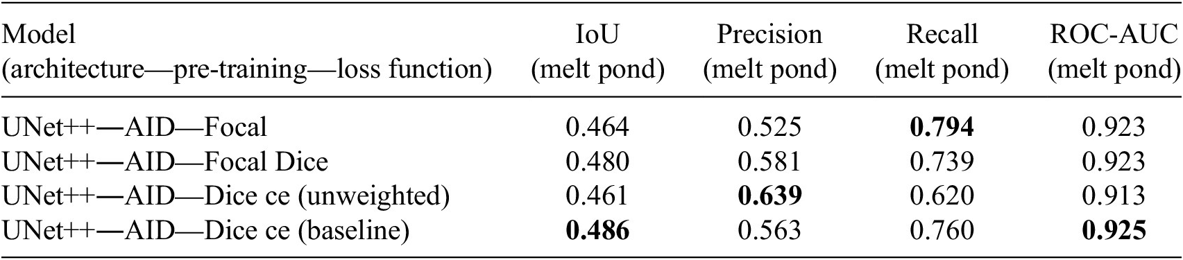
Table 5. Long description
The table consists of five columns and five rows.
Column headers from left to right are: Model (architecture―pre-training―loss function), IoU (melt pond), Precision (melt pond), Recall (melt pond), and ROC-AUC (melt pond).
Row 1: UNet++―AID―Focal. IoU 0.464, Precision 0.525, Recall 0.794 (bold), ROC-AUC 0.923.
Row 2: UNet++―AID―Focal Dice. IoU 0.480, Precision 0.581, Recall 0.739, ROC-AUC 0.923.
Row 3: UNet++―AID―Dice ce (unweighted). IoU 0.461, Precision 0.639 (bold), Recall 0.620, ROC-AUC 0.913.
Row 4: UNet++―AID―Dice ce (baseline). IoU 0.486 (bold), Precision 0.563, Recall 0.760, ROC-AUC 0.925 (bold).
4.3. Analysis of individual predictions
In the following, the predictions of UNet++ pre-trained on AID for individual validation samples are analyzed using the validation model setup. Figure 5 shows model predictions along with their corresponding reference labels and performance measures. We refer to individual images in the figures as samples and identify them by the numbers displayed above each column. Overall, UNet++ successfully captures diverse surface types across varying size, shape, and temperature contrast (e.g., samples 12, 16, and 18). The model performs best on images with large ice floes and well-separated surface classes (e.g., samples 3 and 10). Per-image melt pond IoU values highlight large performance variability across samples, with the best image reaching 0.712 IoU and the lowest scoring 0.076. We observe that the lowest scores are reached by images with small ice floes (samples 6, 7, and 9). Several common error patterns can be observed. Open-water gaps between adjacent floes are frequently misclassified as melt ponds (samples 6, 7, and 9), and the interiors of correctly delineated ponds are sometimes predicted as open water (samples 2, 8, and 20). Melt ponds located at floe edges are also partly misclassified as open water (samples 2 and 8). The error maps in Figure 5 visually reflect the melt pond overestimation found in Section 4.2.
UNet++ prediction results on the validation images reported in Section 3.3. Rows from top to bottom: input images, manual annotations, error map (shows melt pond false positives in red and melt pond false negatives in blue), predictions. Black: melt pond, gray: sea ice, white: open water. Note that while the error map gives a sense of the error patterns, the absolute number of errors is dependent on the occurrences of melt ponds, which shift across the images. The metrics of individual validation samples are reported underneath the respective columns: melt pond IoU (upper number) and feature similarity between the pooled image features and the mean feature vector of the training dataset (lower number).

Figure 5. Long description
The grid is organized into four rows across ten numbered columns.
* Row 1: Input images showing aerial TIR views of sea ice and melt ponds.
* Row 2: Manual annotations where black represents melt ponds, gray represents sea ice, and white represents open water.
* Row 3: Error maps on a black background. Red areas indicate melt pond false positives, and blue areas indicate melt pond false negatives.
* Row 4: UNet++ model predictions using the same black, gray, and white color scheme as the manual annotations.
Beneath each column are two performance metrics. The top number is the melt pond IoU and the bottom number is the feature similarity. From column 1 to 10, the values are:
* Column 1: 0.352 and 0.783.
* Column 2: 0.647 and 0.886.
* Column 3: 0.706 and 0.845.
* Column 4: 0.428 and 0.824.
* Column 5: 0.513 and 0.755.
* Column 6: 0.173 and 0.74.
* Column 7: 0.076 and 0.6.
* Column 8: 0.435 and 0.836.
* Column 9: 0.235 and 0.752.
* Column 10: 0.712 and 0.813.
The last row of Figure 5 shows the cosine similarity between the prediction features and the features of the training set of the validation model. Correlating feature similarity with the respective melt pond IoU reveals a strong positive relationship (Pearson correlation: r = 0.802, Spearman’s rank correlation:
$ \rho $
 = 0.77). This suggests that feature similarity provides a reasonable proxy for expected model performance on unseen images. To make this statement more robust across different training datasets, we perform 3-fold cross-validation and apply the same analysis on the respective validation images and their respective training sets. We find strong positive relationships between feature similarity and performance across all folds (Pearson averaged across folds using Fisher z-transformation: r = 0.72, Spearman’s rank averaged across folds using Fisher z-transformation:
$ \rho $
 = 0.70).
Figures 6 and 7 show predictions of the inference model on images not contained in the labeled dataset. We observe visually improved performance, particularly under challenging image conditions (e.g., sample 24 versus sample 7). These results suggest that model accuracy can be further enhanced with additional labeled training data. The cosine similarity is computed between the individual test images and the training set of the inference model. Results indicate a larger distribution shift for images with small ice floes (samples 12, 25, 26, 27, 30) and higher similarity for images with larger ice floes (samples 14, 15, 21, 28, 29).
UNet++ prediction results on unseen images not contained in the training and validation sets. The feature similarity of each image to the mean feature vector of the training dataset is reported under each respective column (cosine similarity). The images are from the same flights as the labeled data.

Figure 6. Long description
The grid consists of ten vertical columns labeled 11 through 20 at the top.
Top Row: Input images showing grayscale aerial TIR views of sea ice and melt ponds.
Bottom Row: Ten segmented versions of the images above. These predictions use a three-tone color scheme: gray for sea ice, black for melt ponds, and white for open water.
Cosine Similarity Scores: Located at the bottom of each column, representing the feature similarity to the training dataset mean:
Column 11: 0.996
Column 12: 0.990
Column 13: 0.989
Column 14: 0.997
Column 15: 0.997
Column 16: 0.996
Column 17: 0.995
Column 18: 0.996
Column 19: 0.994
Column 20: 0.975
Additional UNet++ prediction results on unseen images not contained in the training and validation sets. The feature similarity of each image to the mean feature vector of the training dataset is reported under each respective column (cosine similarity). The images are from the same flights as the labeled data.

Figure 7. Long description
The grid consists of 20 panels total. The top row contains TIR input images labeled 21 through 30 from left to right. The bottom row shows the corresponding UNet++ prediction results for each image, where features are segmented into distinct black (melt ponds), gray (sea ice), and white (open water) regions.
Below each column is a cosine similarity value representing feature similarity to the training dataset mean. From left to right, the values are:
* Column 21: 0.998
* Column 22: 0.994
* Column 23: 0.993
* Column 24: 0.996
* Column 25: 0.988
* Column 26: 0.991
* Column 27: 0.989
* Column 28: 0.997
* Column 29: 0.997
* Column 30: 0.984
4.4. Label uncertainty
Figure 5 reveals that some of the overestimation of melt ponds occurs at class boundaries, likely due to annotation uncertainty caused by mixed pixels and limited image resolution. Inspired by Bressan et al. (Reference Bressan, Junior, Martins, de Melo, Gonçalves, Freitas, Ramos, Furuya, Osco, de Andrade Silva, Luo, Li, Garcia and Gonçalves2022), we test a method of addressing label uncertainty by reducing the loss weight of pixels close to class boundaries during training. Specifically, we use the Canny edge detector to identify class boundaries in the labels and compute the Euclidean distance of each pixel to its nearest boundary. We exponentially decay these distances by a factor of three and invert them so that pixels closer to class boundaries receive lower weights. This weighting map is then multiplied by the existing class-wise weights in the loss function. Since the Dice cross-entropy loss does not support pixel-wise weighting, we use Focal Dice loss instead. Compared to the baseline Focal Dice training, pixel distance weighting increases precision but reduces recall and melt pond IoU without significantly affecting boundary errors during prediction (Table 6 and Figure 8).
Results of pixel distance loss compared to baseline, reported using 3-fold cross-validation.

Table 6. Long description
The table consists of five columns: Model (architecture—pre-training—loss function), IoU (melt pond), Precision (melt pond), Recall (melt pond), and ROC-AUC (melt pond).
Row 1: UNet++—AID—Focal dice with pixel distance weights. Values are IoU 0.453, Precision 0.592, Recall 0.683, and ROC-AUC 0.921.
Row 2: UNet++—AID—Focal dice (baseline). Values are IoU 0.48, Precision 0.581, Recall 0.739, and ROC-AUC 0.923.
From left to right: Prediction made by a model trained with pixel distance loss, corresponding error map, prediction made by a model without pixel distance loss (the baseline), corresponding error map. The error maps show melt pond false positives in red and melt pond false negatives in blue.

Figure 8. Long description
The figure consists of four square panels arranged horizontally.
* The first panel on the far left shows a prediction from a model trained with pixel distance loss. It features a grayscale map of sea ice with white, gray, and black regions representing different surface types.
* The second panel is the error map for the first model. Against a black background, it displays cyan and red clusters. Cyan represents melt pond false negatives, and red represents melt pond false positives. The red clusters are relatively small and sparse.
* The third panel shows the prediction from the baseline model trained without pixel distance loss. The visual structure is similar to the first panel but with slight variations in the boundaries of the white and gray regions.
* The fourth panel on the far right is the error map for the baseline model. Compared to the second panel, this map shows a higher density of red clusters, indicating a larger number of melt pond false positives when pixel distance loss is not utilized.
4.5. Out-of-distribution generalizability
To test the capability of the model to generalize to flights that were acquired under different conditions, we apply distribution shift measures to the OOD flights described in Section 2.2. The same analysis is applied to the unlabeled test set (Figures 6 and 7), which is referred to as the in-domain set since the images have been sampled from the same flights as the training images. We do not compare against the labeled validation set reported in Figure 5, as these images are predicted using a model trained on less data and thus not directly comparable.
Table 7 reveals that flight 13 exhibits the highest Fréchet similarity to the training data, followed by the in-domain test set and then flight 17. This ranking is consistent with the model’s confidence for the melt pond class. Visual examples from flight 13 illustrate reasonable performance in hazy conditions, with some regions of the images showing overestimation of the open water class (Figure 9). Conversely, Figure 10 shows substantial prediction uncertainty over landfast ice. However, the decrease in Fréchet similarity between the in-domain set and flight 17 is small compared to the significant qualitative degradation. This suggests that the similarity measure does not accurately reflect the extent of this distribution shift.
Assessment of two out-of-distribution flights compared to the in-domain test set. Feature similarity (sim.) is measured as the inverse of Fréchet distance. Per-class confidence (conf.) refers to the mean softmax probability of the predicted class, averaged over all pixels belonging to that class.

Table 7. Long description
The table consists of five columns and four rows including the header.
Column headers from left to right are: Data subset, Feature sim. (Fréchet), Conf. (melt pond), Conf. (sea ice), and Conf. (open water).
Row 1 (In-domain test set): Feature similarity 0.479. Confidence scores are 0.781 for Melt pond, 0.938 for Sea ice, and 0.862 for Open water.
Row 2 (24 July 2022 flight 13): Feature similarity 0.519. Confidence scores are 0.805 for Melt pond, 0.920 for Sea ice, and 0.862 for Open water.
Row 3 (08 August 2022 flight 17): Feature similarity 0.460. Confidence scores are 0.753 for Melt pond, 0.912 for Sea ice, and 0.835 for Open water.
Image samples from flight 13 conducted on 24 July 2022, and predictions with the inference model.

Figure 9. Long description
The multi-panel layout consists of two rows.
Top Row: Five aerial TIR images showing sea ice with melt ponds.
Bottom Row: Five segmented prediction maps corresponding to the input images above. Melt ponds are displayed in black, sea ice in gray and open water in white..
The model predictions in the bottom row precisely trace the boundaries and melt ponds seen in the TIR imagery above.
Image samples from flight 17 conducted on 8 August 2022, and predictions with the inference model.

Figure 10. Long description
The top row contains five aerial TIR showing sea ice.
The bottom row contains five corresponding inference model predictions. These panels use a three-color segmentation scheme consisting of black (melt ponds), gray (sea ice), and white (open water) to map the features from the top row. The model predictions do not match with the input images shown above, indicating that the model struggles to make accurate predictions in these cases.
4.6. Downstream application
The trained model is now applied to a larger set of TIR images from complete helicopter flights to obtain melt pond information on a regional scale. Different melt pond parameters can be derived from the segmentation maps. Important for melt pond studies are the fractions of the different surface components, namely MPF, sea ice fraction (SIF), and open water fraction (OCF). The fractions of these surface components determine, for example, the albedo of the surface and thus affect the energy balance (see Section 1.1).
MPF, OCF, and SIF for each image of the TIR datasets are computed using the following equations:


Here, MP corresponds to the number of melt pond pixels within an image, SI to the number of sea ice pixels, and OC to the number of open water pixels in an image. The segmentation model provides a probability score for each class at each pixel location. For each pixel, we use the probability score of its assigned class to compute an overall mean probability for the image. We then filter out images where this average probability is
$ <0.88 $
 , retaining only high-quality data from the helicopter flights. The threshold was chosen as an initial means to filter low-confidence predictions, based on the observed range of mean probabilities across flights (0.88–0.91). Future work could refine this choice to balance data quality and coverage.
Figure 11 shows a map of the derived MPF for the five helicopter flights from the ATWAICE campaign (Kanzow, Reference Kanzow, Bornemann and Sawadkuhi2023) used to create the labeled dataset. We can see that the MPF generally increases from the marginal ice zone (MIZ) toward the inner ice pack. Only for the flight on 17 July, there is high MPF at the ice margins, in an area of very low ice concentration and very small ice floes (shown as ice-free in the sea ice concentration map of 19 July in Figure 11). There is also significant small-scale variability in all regions. A comparison of the results from different flights shows that the flights of 17, 18, and 19 July have a similar MPF distribution. However, they were also performed in a similar region. For the flight on 30 July, MPF is overall higher than for the earlier flights. This is reasonable, as melting continued throughout the summer. The flight on 30 July was also conducted in a different region, which may further explain the differences in MPF, as sea ice conditions were different.
Map of classified melt pond fraction (MPF) for five helicopter flights during the Polarstern ATWAICE campaign. The flights shown here were conducted on four days in July 2022 as indicated in the map. The background shows sea ice concentration for 19 July 2022 (www.seaice.uni-bremen.de, Spreen et al., Reference Spreen, Kaleschke and Heygster2008). The northern edge of Svalbard can be seen in the lower right corner of the map.

Figure 11. Long description
A geographical map of the Arctic region between 80 and 82 degrees North and 0 to 15 degrees East. The background shows sea ice concentration in shades of white and blue. A legend in the top right corner defines Melt Pond Fraction, or MP F, using a color scale from dark green for 0 to 0.03 to dark red for 0.27 to 1.
Five distinct flight paths are plotted as colored dots.
* In the Northwest, a flight on 17/07 shows a linear path with MPF values mostly in the light green to yellow range, 0.09 to 0.15.
* To the East of that, a flight on 18/07 follows a zig-zag pattern with higher concentrations of orange and red dots, indicating MPF values between 0.18 and 0.27, particularly at its northernmost and southernmost turns.
* Centrally located, a flight on 19/07 shows two short parallel tracks dominated by green and yellow dots.
* In the Southwest, a flight on 30/07 forms a large triangular loop. The western leg is mostly yellow and orange, while the eastern leg shows a concentration of dark red dots near the 81 degree North line.
A scale bar in the bottom left indicates 0 to 75 kilometers. The landmass of Svalbard is visible in the bottom right corner.
We further test the quality of the classification results by splitting the labeled dataset of 21 images into 11 images used for training and the remaining 10 images as reference (considered as truth), as done for the validation model. We train the model and compare the predicted MPF, OCF, and SIF values with the “true” values from the reference dataset.
Table 8 shows the results of this comparison: the model significantly overestimates MPF (
$ +0.11 $
 ), slightly underestimates OCF (
$ -0.04 $
 ), and slightly overestimates SIF (
$ +0.04 $
 ). These results are consistent with the melt pond overestimation observed in Section 4.2. Melt pond classification from visible images has uncertainties of the same order of magnitude, but biases are usually lower (Fuchs, Reference Fuchs2023a).
Fraction values reported on the validation dataset described in Section 3.3, which is composed of 10 diverse images from five helicopter flights. MPF: melt pond fraction; OCF: ocean fraction; SIF: sea ice fraction.

Table 8. Long description
The table consists of four columns and three rows. The header row contains the following column titles: MP F, OC F, and SI F.
Row 1, labeled True, contains the following values:
* MPF: 0.147
* OCF: 0.243
* SIF: 0.757
Row 2, labeled Predicted, contains the following values:
* MPF: 0.253
* OCF: 0.202
* SIF: 0.798
Initialisms are defined as MPF for melt pond fraction, OCF for ocean fraction, and SIF for sea ice fraction.
Note that the model used for the helicopter flights shown in Figure 11 uses all 21 labeled images for training. Using all 21 images for training generally improves the model (compare Figure 5 (only 11 training images) with Figures 6 and 7 (all 21 training images)). Thus, the results in Table 8 are a lower bound for the classification quality, and the actual model performance should be even better.
In summary, the model can provide regional MPF from airborne TIR images with an uncertainty of about 11%. Regional gradients in MPF can be observed in the Fram Strait region in 2022 (Figure 11). In addition, the dataset shows a lot of MPF variability on small spatial scales. Such information is important for the evaluation of satellite-derived MPF, which usually cannot provide such a high spatial resolution as the 1 m dataset presented here.
5. Discussion
The segmentation of sea ice surface classes from summer TIR imagery is a particularly challenging task. The data is characterized by low contrast, labeling uncertainty, and high class imbalance. This means that a certain degree of uncertainty remains inherent to the data, which limits the overall accuracy that can be achieved. Nevertheless, this study demonstrates that deep learning methods can successfully discriminate between sea ice surface types, thereby enabling the use of TIR data in subsequent scientific analyses. Applications of the data and classifications are already being planned, demonstrating their scientific value for the sea ice community. In the following sections, we discuss the results and outline directions for future work.
5.1. Model choice and quantitative analysis
The superior performance of UNet++ in comparison to multi-scale architectures such as PSPNet suggests that fine-grained feature extraction is beneficial for the segmentation of melt ponds. The suboptimal results obtained with PSPNet may be attributed to the inability of multi-scale pooling to sufficiently account for these details. There is no clear evidence indicating whether CNN- or transformer-based methods are more beneficial; for example, both UNet++ and SwinTransformer perform well.
Pre-training on remote sensing data (AID) is advantageous for the downstream task. We consistently observe an improvement of at least one remote sensing pre-training dataset over ImageNet pre-training for all architectures, except SwinTransformers. This aligns with Rolf et al. (Reference Rolf, Klemmer, Robinson and Kerner2024), who argued that incorporating remote sensing-specific characteristics into pre-training can improve downstream performance. Since this study only tests SAM-based architectures with natural pre-training, an interesting future direction is to pre-train these models on remote sensing data to see if their performance improves.
The high class imbalance in the training data negatively affects the models’ ability to perform consistently across classes, resulting in an overestimation of the melt pond class. Despite lower scores on final classification metrics, the fact that the minority class (melt pond) obtains high ROC-AUC values reflects that the models are able to separate melt pond instances from non-melt pond instances. Nevertheless, they fail to classify them correctly under the current decision threshold and instead learn to better classify the majority classes (sea ice and open water). We apply an initial test to adjust per-class decision thresholds, which can improve precision by more than 0.06 with no significant change to the melt pond IoU. Further exploration of this approach will be of particular interest to users seeking high precision. Full details are provided in the Supplementary Material.
We also find that an unweighted loss function yields higher melt pond precision. This indicates that including class weights in the loss term results in overcompensation for the melt pond class. For applications requiring higher precision, users can further adjust the class weights in the loss term. The finding that Focal loss, which operates at the pixel level, performs worse than a combination of pixel- and region-level loss functions indicates that incorporating spatial context is beneficial for the task.
5.2. Generalizability
The model presented here generally performs better on images with larger ice floes and shows greater uncertainty on smaller ones. It performs reasonably on hazy images but requires retraining for applications over landfast ice.
Within the labeled dataset, the correlation assessments of this study support previous findings of Fuller et al. (Reference Fuller, Millard and Green2022) that feature similarity correlates with model performance. However, applying feature similarity measures to hazy images produces unexpectedly high values. For landfast ice images, both feature similarity and model confidence are lower than for the in-domain dataset, consistent with poor visual results, although the drop in segmentation quality is more pronounced. These results suggest that feature similarity and model confidence capture some types of domain shifts but may miss task-relevant differences. They can serve as efficient initial indicators of generalizability, but visual inspection remains essential. Future work could explore domain similarity measures that better capture task-specific features.
5.3. Limitations and future work
One limitation of this study is the small amount of labeled training data, which likely limits model performance. To reduce the need for annotating more TIR images and with regard to the large unlabeled dataset available, future work could explore semi-supervised approaches (e.g., Zhu and Goldberg, Reference Zhu and Goldberg2022). In the Supplementary Material, we conduct initial experiments using the DMT algorithm, which demonstrate that semi-supervised training can improve melt pond IoU by about 4% and show promise for future research. Additionally, the annotation process could be presented as a data challenge at machine learning conferences, provided that evaluations are carefully conducted using expert labels. Other directions include super-resolution and multi-source training approaches. Using the RGB information of optical sensors as additional training data is expected to be particularly useful. This is currently being challenged by the different geometries of the sensor types, which require image registration.
Further evaluation is needed to assess the generalizability of the model. This is currently limited by the availability of reference datasets. It will be essential to collect additional data from diverse geographical regions and ice regimes. Many individual factors may influence the geometry of melt ponds, such as ice type. Melt ponds tend to be interconnected on first-year ice, while the ice topography can enforce more variable structures on multiyear ice, for example, when bounded by ridges. Similarly, larger area fractions may be covered by melt ponds on first-year ice, because it is usually flatter than multiyear ice, which is more deformed. This may restrict generalizability, especially as climate change progresses and larger areas of the Arctic are covered by first-year ice rather than multiyear ice. However, the relationship between MPF and ice type is complex and not fully understood (Niehaus et al., Reference Niehaus, Spreen, Istomina and Nicolaus2025). It is also important to collect more data from various stages of melt pond evolution, as melt pond coverage fluctuates throughout the season (Landy et al., Reference Landy, Ehn and ShieldsMand Barber2014; Webster et al., Reference Webster, Rigor, Perovich, Richter-Menge, Polashenski and Light2015; Niehaus et al., Reference Niehaus, Spreen, Istomina and Nicolaus2025), and especially the early and late parts of the season are not covered by the dataset. Similar campaigns with the TIR VarioCAM measurement system are planned and can be used to address this need in future studies.
Another limitation is that the model is trained and tested on the original image geometry without georeferencing (see Section 2.3), which implies slight distortions at image boundaries. How much this affects the fractional results reported in Section 4.6 is not further tested here.
5.4. Downstream applications
The resulting TIR segmentations can be used to complement optical data in the analysis of melt pond coverage. In a future study, the MPF results can be compared with classifications of visible imagery collected simultaneously during the helicopter flights. A first visual comparison reveals that there are differences in the representation of melt ponds in TIR compared to optical imagery. For instance, a greater number of melt ponds can be observed in optical imagery. The reasons for this are not further analyzed here.
Other potential pathways include the validation of TIR satellite data for melt pond detection (Thielke et al., Reference Thielke, Huntemann, Hendricks, Jutila, Ricker and Spreen2022). The dataset can also be explored to reveal thermal properties of melt ponds on a regional scale. The full potential of the dataset is to be explored in future work.
6. Conclusion
This work presents a dataset of helicopter-borne TIR images of melt ponds on Arctic sea ice and evaluates deep learning models for surface-type segmentation. Among the tested architectures, UNet++ pre-trained on AID achieved the best performance, with a melt pond IoU of 0.486, precision of 0.563, and recall of 0.760. For the sea ice and open water classes, the model reached IoUs of 0.764 and 0.660, respectively. On the validation dataset, we observed an overestimation of MPF by 11% (bias) and lower uncertainties of about 4% for sea ice and open water fractions. The automated workflow, including data processing, classification, and fraction calculation, is made publicly available.
Abbreviations
- CNN
-
convolutional neural network
- DMT
-
dynamic mutual training
- FCN
-
fully convolutional network
- IoU
-
intersection over union
- MIZ
-
marginal ice zone
- MLP
-
multi-layer perceptron
- MODIS
-
moderate resolution imaging spectrometer
- MPF
-
melt pond fraction
- OCF
-
open water fraction
- OOD
-
out-of-distribution
- PSPNet
-
pyramid scene parsing network
- ROC
-
receiver operating characteristic
- ROC-AUC
-
receiver operating characteristic area under the curve
- SAM
-
segment anything
- SIF
-
sea ice fraction
- TIR
-
thermal infrared
- UAV
-
unmanned aerial vehicle
- ViT
-
vision transformer
Open peer review
To view the open peer review materials for this article, please visit http://doi.org/10.1017/eds.2026.10072.
Supplementary material
The supplementary material for this article can be found at http://doi.org/10.1017/eds.2026.10072.
Acknowledgements
We are grateful to Ulf Krumnack, who supervised M.R.’s bachelor’s thesis that preceded this work. We would like to thank Anthony Fuller and Francis Pelletier for their insightful comments. Our thanks also go to the entire Remote Sensing of Polar Regions group at IUP Bremen, as well as to Julia Kaltenborn, for insightful discussions. We thank all persons involved in the Polarstern ATWAICE campaign (Kanzow, Reference Kanzow, Bornemann and Sawadkuhi2023), and here especially the pilots, the sea ice team onboard, and Gerit Birnbaum for the helicopter work support. We thank the journal editor and the reviewers for their comments and feedback, which helped to improve the manuscript.
We acknowledge the use of GitHub Copilot (free version), DeepL Write (free version), and ChatGPT (free version) to optimize specific code functions, correct grammatical errors, and rephrase parts of the text. The outputs were thoroughly validated and the authors take full responsibility for the final content. The tools were not used to generate facts or citations.
Author contributions
Conceptualization: G.S., M.R.; Data curation: G.S., L.B., M.H.; Funding acquisition: G.S.; Investigation: G.S., M.R.; Methodology: D.W., M.R.; Software: M.H., M.R.; Supervision: D.W., G.S.; Writing original draft: M.R.; Writing review and editing: G.S., M.H., D.W., L.B. All authors approved the final submitted draft.
Competing interests
The authors declare none.
Data availability statement
The helicopter data that support the findings of this study are openly available on PANGAEA at https://doi.pangaea.de/10.1594/PANGAEA.971908. Replication code, training data, and fraction results can be found on GitHub: https://github.com/marlens123/tir_surface_segmentation.
Ethics statement
The research meets all ethical guidelines, including adherence to the legal requirements of the study country.
Funding statement
This research was supported by grants from the Deutsche Forschungsgemeinschaft (DFG, German Research Foundation) through the Transregional Collaborative Research Center TRR 172 “ArctiC Amplification: Climate Relevant Atmospheric and SurfaCe Processes, and Feedback Mechanisms (AC)
$ {}^3 $
 ” (project number 268020496). The work was also supported by a fellowship from the German Academic Exchange Service (DAAD).












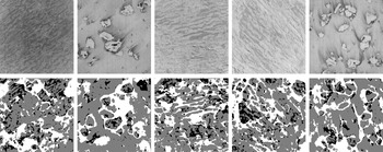




 Open access


Comments
17 November 2024
Subject: Submission of Manuscript Titled “Deep Learning for the Detection of Melt Ponds on Sea Ice from Airborne Infrared Images”
Dear Members of the Editorial Team,
I am pleased to submit our manuscript, titled “Deep Learning for the Detection of Melt Ponds on Sea Ice from Airborne Infrared Images” for consideration in Environmental Data Science.
We believe this research contributes to the ongoing advancements in environmental data science and offers practical insights for researchers working with melt pond data. We believe this work will be of particular interest for readers focused on polar regions, climate science, deep learning applications, and remote sensing.
This manuscript has not been published or submitted elsewhere, and all authors have approved the submission to Environmental Data Science. Additionally, we have adhered to your guidelines on formatting and submission.
Thank you for considering our submission. I look forward to the possibility of collaborating with you and your reviewers to further refine our work.
Sincerely,
Marlena Reil
marlena1@gmx.de