

1. Introduction
Early experiences and psychosocial stimulation during early childhood (i.e., the first 5 years of life) are crucial determinants of better outcomes in subsequent stages of life (Nores et al., Reference Nores, Vázquez, Gustafsson-Wright, Osborne, Cuartas and Lambiris2024). Basic stimulation activities (playing, reading and singing with a child) can improve a child’s ability to think, communicate and connect with others (Black et al., Reference Black, Walker, Fernald, Andersen, DiGirolamo, Lu, McCoy, Fink, Shawar, Shiffman, Devercelli, Wodon, Vargas-Barón and Grantham-McGregor2017). As such, one public policy response to achieve this goal has been to invest in early childhood development programs, particularly parenting programs. Home visits by community workers to local families are a promising way to deliver parenting programs, given their success in improving parenting practices and child development (Berlinski & Schady, Reference Berlinski and Schady2015; IDB, 2024; Nores et al., Reference Nores, Vázquez, Gustafsson-Wright, Osborne, Cuartas and Lambiris2024). In general, these visits aim to encourage stimulating activities, good health practices and positive disciplinary strategies within the home, resulting in an improvement in environmental quality and, therefore, in children’s cognitive and socioemotional development.
A small-scale home visiting program in Jamaica targeted at children 6–24 months achieved short-term impacts on cognition and language and longer-term effects on education, behaviors, employment and earnings (Gertler et al., Reference Gertler, Heckman, Pinto, Chang, Grantham-McGregor, Vermeersch and Wright2021), while a recent meta-analysis on 18 replications of this model showed large child development impacts in pilot studies.Footnote 1
In Latin America (LAC), the Jamaican model has been adapted and gradually scaled up in half a dozen countries, showing positive impacts that decrease with scale. In Colombia, for example, the model was integrated into the existing national conditional cash transfer program Familias en Accion. The initial impacts on cognition (0.26 standard deviations (SD)) and receptive language (0.22 SD) after 24 months of home visits were calculated to fill a third of the gap in cognition between children living in an extremely disadvantaged environment and children living in middle-class families in Bogota (Attanasio et al., Reference Attanasio, Fernandez, Fitzsimons, Grantham-McGregor, Meghir and Rubio-Codina2014). Yet, they faded away after 2 years (Andrew et al., Reference Andrew, Attanasio, Fitzsimons, Grantham-McGregor, Meghir and Rubio-Codina2018).
This model was further adapted later to be implemented nationwide in Peru and evaluated using a randomized controlled trial (RCT). After 3 years of operation, the Peruvian Cuna Más program was delivering weekly home visits to over 67,000 vulnerable pregnant women and children under age 3 years in rural areas. Evaluation findings showed impacts on development of 0.10 SD after 2 years of intervention (Araujo, Marta, et al., Reference Araujo, Marta, Grantham-McGregor, Fabiola, Rubio-Codina and Schady2021). Since then, the Jamaica curriculum – now known as Reach Up and Learn (RU) – has been adapted in Ecuador to strengthen a long-standing nationwide family support program, and in Panama to reach vulnerable Indigenous populations. Various elements of the RU training and supervision packages have also been used in other low- and middle-income countries (LMICs), including Nicaragua, Panama, Ecuador and the Brazilian cities of Fortaleza, São Paolo and Boa Vista (Jervis et al., Reference Jervis, Coore-Hall, Pitchik, Arnold, Grantham-McGregor, Rubio-Codina and Baker-Henningham2023; IDB, 2024), becoming the gold standard of home-visiting programs in LMICs.
Understanding the benefits and costs of early childhood development (ECD) programs is crucial when choosing which policies to implement, as some programs have greater benefit–cost (BC) ratios than others: BC ratios of home visits at scale in LMICs range from 5.4 in Peru (Araujo, Rubio-Codina, & Schady, Reference Araujo, Rubio-Codina and Schady2021) to 11.7 in Nicaragua (Lopez Boo et al., Reference Lopez Boo and Kamei2025), while for at-scale childcare, they have been calculated to be 6.2 in Nicaragua (Hojman & Lopez Boo, Reference Hojman and Lopez Boo2022). On the other hand, BC ratios for preschool programs range from 3.4 in Colombia (Berlinski & Schady, Reference Berlinski and Schady2015), 11 in Argentina (National Bureau of Economic Research, Reference Berlinski, Cruces, Galiani, Gertler and Gonzalez2025) and 18 in Mozambique (Bassi et al., Reference Bassi, Besbas, Dinarte, Ravindran and Reynoso2025). It is, however, important to note that positive impacts on child development outcomes for childcare appear to emerge only under two conditions: when service quality is relatively high, and when services are targeted at vulnerable populations. As this article focuses on LMICs, the relevant literature is largely encouraging – rigorous at-scale trials generally report positive effects (Hojman & Lopez Boo, Reference Hojman and Lopez Boo2022). In higher-income contexts, however, childcare has been shown to have no effect or even negative effects, particularly in large-scale studies of high-quality provision for children aged 0–2 years. Evidence of null or adverse impacts comes from Italy (Carta & Rizzica, Reference Carta and Rizzica2018; Fort et al., Reference Fort, Ichino and Zanella2020), Quebec (Baker et al., Reference Baker, Gruber and Milligan2008, Reference Baker, Gruber and Milligan2019) and Denmark (Gupta, Reference Gupta and Simonsen2010). Crucially, negative impacts tend to appear among better-off target populations – as observed in the Quebec and Italy studies – and in contexts where the quality of alternative care at home (the counterfactual) is high relative to that of the program itself.
Both benefit–cost ratios and internal rates of return require either longitudinal surveys or administrative data in adulthood to know long-run impacts of early childhood interventions. Otherwise, assumptions about the long-term impacts of such interventions will be needed on how, for instance, the short-run impact (e.g., in standard deviations) translates into wage increases (Kline & Walters, Reference Kline and Walters2016). However, very few studies analyze long-term benefits in terms of completed education, health, crime and labor income, and all come from rich countries (Heckman et al., Reference Heckman, Hyeok Moon, Pinto, Savelyev and Yavitz2010; Havnes & Mogstad, Reference Havnes and Magne2011).
More recently, García et al. (Reference García, Heckman, Ermini Leaf and Prados2020) investigate the social benefits and costs of two related ECD programs implemented in North Carolina for highly vulnerable children: The Carolina Abecedarian Project (ABC) and the Carolina Approach to Responsive Education (CARE). Both programs were evaluated through randomized controlled trials (RCTs), launched in the 1970s, and followed participants through age 30 years. Their analysis yields one of the most widely cited figures in the ECD literature: a tax-adjusted internal rate of return (IRR) of 13.7% per annum and a 7.3 benefit–cost ratio.
The main contribution of this study is to leverage existing longitudinal data – collected at ages 22 and 31 – from an RCT of a home-visiting ECD program in Jamaica to calculate its IRR and benefit–cost ratio. In doing so, it fills an important gap in the literature: to our knowledge, this is the first IRR estimate derived from an LMIC setting, extending the evidence base beyond the high-income country context in which most prior estimates – including the ABC/CARE and other landmark US studies – have been generated. To assess the reliability of our findings, we conduct a range of robustness checks, including sensitivity analyses on key assumptions. We further estimate the IRR separately by gender, shedding light on the heterogeneity of returns and allowing for a direct comparison with evidence from the United States, where male and female returns to early childhood investment have been shown to differ substantially (Heckman et al., Reference Heckman, Hyeok Moon, Pinto, Savelyev and Yavitz2010; García et al., Reference García, Heckman, Ermini Leaf and Prados2020).
2. The Jamaica early childhood stimulation intervention study
The Jamaican home visiting program was designed in the 1970s and 1980s and aimed to build parents’ skills to promote child development outcomes. The intervention study was conducted in 1987–1989 and involved 129 chronically malnourished children 9–24 months old from poor neighborhoods in Kingston. Their enrollment was conditioned on stunting due to its correlation with poor cognitive development (Gertler et al., Reference Gertler, Heckman, Pinto, Zanolini, Vermeerch and Walker2014). The 129 children were stratified by age and gender, then, within each stratum, they were randomly assigned to one of four groups: (1) psychosocial stimulation (N = 32); (2) nutritional supplementation (N = 32); (3) both psychosocial stimulation and nutritional supplementation (N = 32); and (4) a control group that received neither (N = 33). The intervention lasted 2 years, and children in all groups were granted access to free health care. The nutritional intervention applied to groups 2 and 3, which consisted of a weekly supply of nutritional supplements. The psychosocial stimulation intervention was applied to groups 1 and 3, which consisted of weekly 1-hour free home visits with a curriculum designed to develop child cognitive, language, fine-motor and socioemotional skills (more detailed information about the intervention can be found in Walker et al. (Reference Walker, Powell and Grantham-McGregor1990)).
During these visits, a community health workerFootnote 2 engaged mothers to interact with their children. The main goal of these visits was to improve the quality of mother–child interactions. An initial evaluation of the program showed benefits on overall development of 13.4 IQ points or 0.88 standard deviations (SDs) – after 24 months of home visits (Grantham-McGregor et al., Reference Grantham-McGregor, Powell, Walker and Himes1991). These impacts translated to better academic attainment, reduced depression, less violent behavior and earnings that were around 24.6% higher when participants were 22 years old, and 45% higher at age 31 years (Gertler et al., Reference Gertler, Heckman, Pinto, Zanolini, Vermeerch and Walker2014, Reference Gertler, Heckman, Pinto, Chang, Grantham-McGregor, Vermeersch and Wright2021; Walker et al., Reference Walker, Chang, Vera-Hernandez and Grantham-McGregor2011).
Today, the Reach Up program is a play-based intervention based on the Jamaican curriculum and relying on additional materials to support program implementation (e.g., adaptation, training and supervision). Designed for delivery by facilitators who have finished primary school, at minimum, and emphasizing interactions, RU has been replicated in several LMICs and has consistently shown short-term benefits on cognition and language (Grantham-McGregor & Smith, Reference Grantham-McGregor and Smith2016; Jervis et al., Reference Jervis, Coore-Hall, Pitchik, Arnold, Grantham-McGregor, Rubio-Codina and Baker-Henningham2023).Footnote 3 Even if evidence on medium-term benefits of these experiences is generally not yet available, the program is still a source of inspiration for many parenting programs in LMICs.
3. Methods
To estimate IRR for social interventions, one should assign dollar net values to social outcomes (e.g., reduced crime, improved health and higher future earnings) so they can be discounted to the present and compared to costs like a standard financial IRR (Nas, Reference Nas2016). Due to the simplicity of this approach, it has been commonly used for estimating the profitability of social programs and interventions. Heckman et al. (Reference Heckman, Hyeok Moon, Pinto, Savelyev and Yavitz2010), for example, estimated the IRR of the High Scope Perry Preschool Program, an early intervention program targeted toward disadvantaged African American children.
To estimate the IRR of the Jamaican Home Visit program (Grantham-McGregor et al., Reference Grantham-McGregor, Powell, Walker and Himes1991), our approach will then rely on the traditional Net Present Value (NPV) calculation of benefits. Based on Gertler et al. (Reference Gertler, Heckman, Pinto, Chang, Grantham-McGregor, Vermeersch and Wright2021) that did not find significant impacts of the nutritional component of the intervention, we also combined the stimulation-only arm and the stimulation-and-nutrition arm for the benefits, but the costs are only derived from the stimulation-only treatment arm.
Using the program costs data published in Zhou et al. (Reference Zhou, Heckman, Liu, Lu, Chang and Grantham-McGregor2023) and wage impacts estimated by Gertler et al. (Reference Gertler, Heckman, Pinto, Zanolini, Vermeerch and Walker2014, Reference Gertler, Heckman, Pinto, Chang, Grantham-McGregor, Vermeersch and Wright2021), we estimated the IRR following García et al. (Reference García, Heckman, Ermini Leaf and Prados2020). The formal definition can be written as follows:

where CF t is the Cash Flow at period t, and It is the initial investment (I 0 = I 1 = $48,962 and I t ≥ 2 = 0; see the next section for how we calculated the $48,962 figure for the initial investments).
3.1. Costs
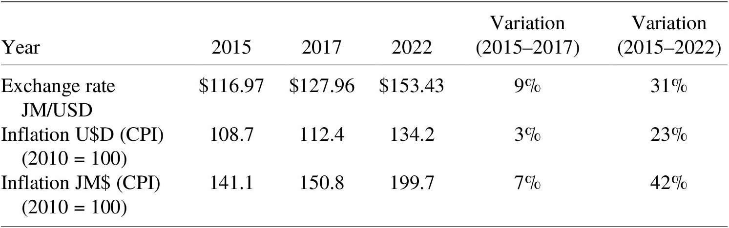
Table 11 in Zhou et al. (Reference Zhou, Heckman, Liu, Lu, Chang and Grantham-McGregor2023) reports the costs of the Jamaican Home Visit program in 2015 US dollars. The original costs of the program were expressed in 1988 Jamaican dollars and were adjusted for inflation and exchange rate variations. Using the exchange rate and consumer price index data from the World Bank, we further adjusted the Zhou et al. (Reference Zhou, Heckman, Liu, Lu, Chang and Grantham-McGregor2023) values to 2017 US dollars (see Appendix A for details on costing adjustments to 2017 USD). Table 1 reports the breakdown of total program cost per year per child. The yearly cost of the program was $48, 962.56 US dollars; since the whole intervention lasted 2 years, the total cost was $97,925 US dollars.Footnote 4
Annual program costs Jamaican Home Visit program (stimulation arms)

Table 1. Long description
Reports 2017 USD program costs. Total annual cost: $48,962.56 ($777.18 per child). Fixed costs: $16,381.87 ($260.03 per child), comprising expert fee $12,579.39 ($199.67) and supplies/facilities $3,802.48 ($60.36). Variable costs: $32,580.69 ($517.15 per child), comprising personnel cost $30,439.39 ($483.16) and toy-making/materials $2,141.30 ($33.99).
a Values expressed in 2017 US dollars based on Zhou et al. (Reference Zhou, Heckman, Liu, Lu, Chang and Grantham-McGregor2023). N = 63 children from groups (1) and (3) of RCTs that received stimulation (64–1 child lost to follow-up).
3.2. Benefits
3.2.1. Earnings
Benefits estimation was based on previous impact evaluations of the program. We did not forecast life-cycle earnings, but we rather used Gertler et al. (Reference Gertler, Heckman, Pinto, Zanolini, Vermeerch and Walker2014, Reference Gertler, Heckman, Pinto, Chang, Grantham-McGregor, Vermeersch and Wright2021) that estimated the effect of the program on different labor market indicators as input. Due to data constraints, in this article we solely focus on the wage impacts. The first long-run impact evaluation found that participants’ earnings increased by 24.6% by age 22. Earnings were 37% higher by age 31 in the second long-run evaluation.
Using these results, we estimated an income stream based on the following assumptions, several of which are subsequently subject to sensitivity analyses:
-
1. Participants started working at the age of 20 and retired at 65, which yields a 46-year working life.
-
2. During the first 11 years of working life, the participants earn a wage 24.6% higher than the control group; by the age of 31 and until they retire, the wage premium rises to 37%.
-
3. The benchmark wage is the control group wage reported in previous studies adjusted by inflation and exchange rates to 2017 US dollars.
-
4. The income stream is a constant value with the exception of a discrete jump at age 31. We include a linear trend growth in the sensitivity analysis.
-
5. Impact estimates already account for labor force participation rate and unemployment rate.
3.2.2. Forecasting other life-cycle benefits
Forecasting other life-cycle benefits is usually done when evaluating the impact of ECD programs due to the wide range of benefits from early intervention. Heckman et al. (Reference Heckman, Hyeok Moon, Pinto, Savelyev and Yavitz2010) do this for the Perry program evaluation: they account for crime reduction benefits and discuss other potential program impacts that are not easily quantified, including the utility of committing crime, leisure, marital and parental outcomes, the program’s contribution to child care, wealth accumulation, social life, improved health and longevity and potential intergenerational effects of the program. Following similar methods, García et al. (Reference García, Heckman, Ermini Leaf and Prados2020) include health improvement effects, crime reduction and parental labor income as non-income-related benefits of The Carolina Abecedarian Project and the ABC/CARE. For the Jamaica study, we are unfortunately unable to take this approach due to the lack of data on adult outcomes related to health, mental health and crime, as well as the methodological challenges associated with monetizing these outcomes.
4. Results and sensitivity analysis
Table 2 presents the benefit–cost ratios from the Jamaica study under different discount rates and wage return assumptions, both including and excluding the costs of schooling.
Benefit–cost ratio Jamaican home visit program (ratio and 90% CI for wage impacts): full time versus all types of jobs

Table 2. Long description
At discount rates 2%–12%, reports BC ratios and 90% CIs for Return 1 (full-time jobs) and Return 2 (all jobs), with and without schooling costs. Return 1 BC ratio falls from 18.8 (2%) to 0.6 (12%); with schooling costs, from 10.6 to 0.7. Return 2 BC ratio falls from 19.5 to 0.7; with schooling costs, from 11.0 to 0.7. IRR: 11.2% for Return 1 (90% CI 0.0%–14.5%; 10.4% with schooling costs); 11.6% for Return 2 (90% CI 3.4%–14.6%; 10.7% with schooling costs). Monthly control-group income (2017 USD): Return 1, $307.63 before age 31 and $363.83 from 31; Return 2, $254.39 before age 31 and $363.83 from 31.
a Return 1: 24.6% earnings impact up to age 31 years (estimated return for full-time jobs derived from Gertler et al., Reference Gertler, Heckman, Pinto, Zanolini, Vermeerch and Walker2014), followed by a 37% impact thereafter (Gertler et al., Reference Gertler, Heckman, Pinto, Chang, Grantham-McGregor, Vermeersch and Wright2021).
b Return 2: 35% earnings impact up to age 31 years (estimated return for all types of jobs derived from Gertler et al., Reference Gertler, Heckman, Pinto, Zanolini, Vermeerch and Walker2014), followed by a 37% impact thereafter (Gertler et al., Reference Gertler, Heckman, Pinto, Chang, Grantham-McGregor, Vermeersch and Wright2021).
c Calculation of mean income for control group based from Table 1, row1, column 2 of Gertler et al. (Reference Gertler, Heckman, Pinto, Zanolini, Vermeerch and Walker2014) and Table 1, row 2, column 3 of Gertler et al. (Reference Gertler, Heckman, Pinto, Chang, Grantham-McGregor, Vermeersch and Wright2021).
Our preferred specifications are presented in bold.
We use two wage returns that stem from variations in the estimated impact on earnings across different age brackets of the income stream. Because we are unable to forecast life-cycle earnings directly, Return 1 assumes a constant 24.6% earnings impact up to age 31 (i.e., the estimated return for full-time jobs derived from taking the log transformation of the treatment effect on average log earnings reported in Table 1, row 1, column 2 of Gertler et al., Reference Gertler, Heckman, Pinto, Zanolini, Vermeerch and Walker2014), followed by a constant 37% impact thereafter (based on Gertler et al., Reference Gertler, Heckman, Pinto, Chang, Grantham-McGregor, Vermeersch and Wright2021). For more details on the calculation of the average wage impact, see Appendix C. On the other hand, Return 2 assumes a 35% impact (i.e., log transformation on the treatment effect on average log earnings in Table 1, row 1, column 1 in Gertler et al., Reference Gertler, Heckman, Pinto, Zanolini, Vermeerch and Walker2014) up to age 31 because it includes all types of jobs, not exclusively full-time jobs, also followed by a 37% impact thereafter.
Note that these calculations assume constant incomes for both the treatment and control group, with a discrete jump happening at different rates for both groups at age 31.Footnote 5
We are unfortunately unable to construct confidence intervals for our IRR estimates given the lack of access to microdata; however, in an attempt to provide ranges for our estimates, Table 2 also presents confidence interval (CI) estimations, based on the 95% confidence intervals of the treatment effect on wages for ages 22 and 31. Treatment effects confidence intervals are not reported in the original papers, so we based our estimates on the reported sample size, t-stat (when reported), and estimated effects on wages in Gertler et al. (Reference Gertler, Heckman, Pinto, Zanolini, Vermeerch and Walker2014, Reference Gertler, Heckman, Pinto, Chang, Grantham-McGregor, Vermeersch and Wright2021).
For Gertler et al. (Reference Gertler, Heckman, Pinto, Zanolini, Vermeerch and Walker2014), sample size and treatment effects are reported, so we estimated the t-stat assuming a t-distribution with a two-sided tail. Once we estimate the t-stat, the calculation of the standard deviation, standard error and confidence intervals (CIs) can be easily obtained. Using this one-sided 95% CI (which is equivalent to a two-sided 90% confidence interval for symmetric distributions), we calculate the CI for the impacts of Returns 1 and 2. We find that the mean IRR for Return 1 is 11.2%, with a range between 0% and 14.5%, while for Return 2 the mean is 11.6%, with a range between 3.4% and 14.6%. Both estimates fall ~2 percentage points below the 13.7% IRR reported by García et al. (Reference García, Heckman, Ermini Leaf and Prados2020) for the Abecedarian project.Footnote 6
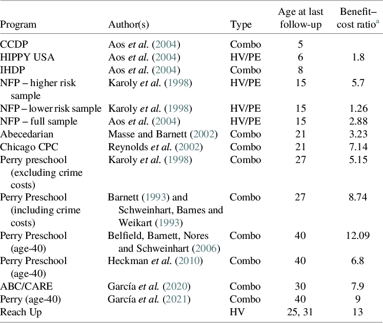
Additionally, at a conservative discount rate of 3%, the benefit–cost ratio is 12.8 (13.4 using Return 2), compared to 4.5 (4.8 using Return 2) at a moderate discount rate of 6%. We further compare our benefit–cost ratio estimates with a full list of benefit–cost ratios from the literature in Table B1 (Appendix B) and show that the Jamaican benefit–cost ratio is greater than any other estimate in the literature, including the latest estimate for Perry (García et al., Reference García, Bennhoff, Leaf and Heckman2021), which stands at 9, and an older estimate for Perry at age 40 (Belfield et al., Reference Belfield, Nores, Barnett and Schweinhart2006), which stands at 12.9. It is important to note that in Belfield et al. (Reference Belfield, Nores, Barnett and Schweinhart2006), most program gains come from reduced crime among males, which further suggests that our estimates are conservative. Moreover, when comparing our estimates with the benefit–cost ratio based only on earnings benefits from these two studies, the benefit–cost ratios are 4.25 for Perry (age 40) based on Table 9 in Belfield et al. (Reference Belfield, Nores, Barnett and Schweinhart2006) and 3.0 for the Abecedarian (Table 3, García et al., Reference García, Bennhoff, Leaf and Heckman2021). Our preferred analysis accounts for future schooling costs associated with the documented improvements in schooling trajectories. Gertler et al. (Reference Gertler, Heckman, Pinto, Chang, Grantham-McGregor, Vermeersch and Wright2021) found a treatment effect of 0.77 additional years of education for the whole sample (0.25 for men and 1.33 additional years for women). We therefore estimate the cost of one additional year of schooling using the per-capita expenditure figures reported by the Jamaican Ministry of Education, Skills, Youth and Information, finding that both BC ratios and IRR decrease, as shown in Table 2 (see Appendix D for details): estimates of the IRR including schooling cost are 10.4% with a 90% CI of (−3.5% to 13.9%) and a 10.7% (0.77% to 14.0%) IRR for returns 1 and 2, respectively.
Sensitivity analysis: varying returns based on different samples (full time non migrants, all types of jobs nonmigrants)

Table 3. Long description
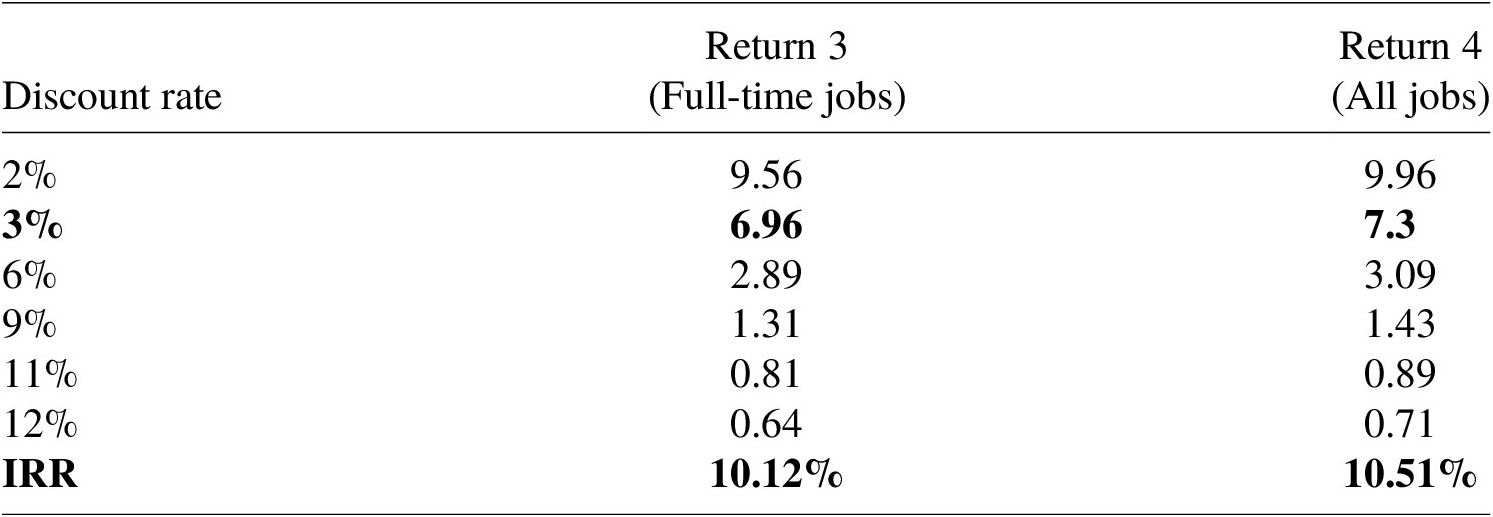
Return 3 (full-time jobs, non-migrant sample) BC ratio falls from 9.56 (2%) to 0.64 (12%), IRR 10.12%. Return 4 (all jobs, non-migrant sample) BC ratio falls from 9.96 to 0.71, IRR 10.51%.
Our preferred specifications are presented in bold.
4.1. Sensitivity analysis
We conduct a sensitivity analysis accounting for the diversity of possible subsamples and returns combinations (Table 3) and for different labor market entry ages and retirement ages (Table 4). Throughout these analyses, we present results across five discount rates (2%, 3%, 6%, 9% and 12%), as BC ratios are sensitive to the choice of discount rate and always take into account the estimates from the last column for each Return from Table 2 (e.g., with schooling costs).
Sensitivity analysis: different labor market entrance and retirement ages

Table 4. Long description
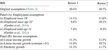
Original assumptions: IRR 10.4% (Return 1), 10.7% (Return 2). Panel A (employment assumptions): employed since age 18 → 11.1%/11.6%; employed since age 22 → 9.8%/10.1%; employed until age 31 only (no extrapolation) → 7.4%/8.2%. Panel B (income assumptions): linear income growth to retirement → 11.3%/11.5%; linear growth until 31 then constant → 11.0%/10.7%; elasticity growth specification → 11.3%/11.7%.
a An additional sensitivity analysis could have been conducted by adding up to two extra earnings data points for ages 18–22, drawn from the first, current and last job modules in Gertler et al. (Reference Gertler, Heckman, Pinto, Zanolini, Vermeerch and Walker2014) questionnaire. We did not pursue this, however, for two reasons: (i) treatment effects on first job earnings were nonsignificant (Table S6, Gertler et al., Reference Gertler, Heckman, Pinto, Zanolini, Vermeerch and Walker2014), and (ii) last and current job also coincide for the majority of the sample. No other data point can be added from the second follow-up (Gertler et al., Reference Gertler, Heckman, Pinto, Chang, Grantham-McGregor, Vermeersch and Wright2021), as only one earnings observation was collected at age 31.
For Return 3, we again employ the full-time jobs sample up to age 31, but beyond age 31 we apply the estimated effect derived from the nonmigrant sample (42%) rather than the full sample. Return 4 is analogous to Return 3 but encompasses all types of jobs in the initial years. Across all specifications, the IRR estimates are robust to variations in sample composition and returns definition, ranging from 10.12% to 10.51%.
Table 4 presents the IRR estimates under alternative employment assumptions (Panel A) and income stream specifications (Panel B, see Appendix C). In our original specifications in Tables 2 and 3, we assumed that employment began at age 20, while the first observed income data point in the Jamaica follow-up survey is at age 22. We also assumed a two-tranche constant impact. In Table 4, we present: (a) a start age of 18 (the standard assumption in the literature; (b) employed beginning at age 22 (the age at which observed income data are available for this sample); (c) employed until age 31 (the most conservative assumption); row (d) and (e) estimates assume a linear income growth under different specifications; and (f) where results are based on an elasticity of income growth.
Turning to the results, assuming employment begins at age 20 rather than 22 (row b) implies a slightly larger IRR (10.4% and 10.7%, compared to 9.8% and 10.1%, respectively). If we limit the analysis to the available data from the two adult follow-up surveys without extrapolating income trends, the IRR estimate is 7.4% for Return 1 and 8.2% for Return 2 (row c). Note that this assumption is particularly conservative, as it implies no income imputation beyond age 31, yet still yields a high IRR. Turning to Panel B of Table 4, we find that if the income stream continues to grow at the same rate until age 65, the IRR would be 11.3% and 11.5% for Returns 1 and 2, respectively (row d). Under the assumption that linear earnings growth occurs only until age 31, after which the income stream remains constant, the IRR is 11.0% and 10.7% (row e). Finally, under the elasticity growth specification, the results are broadly similar; differences arise from the interplay between the varying evolution patterns of income and the discount rate. Income accruing at later ages is heavily discounted, resulting in a smaller present value of benefits.
5. Discussion and gender effects
Gertler et al. (Reference Gertler, Heckman, Pinto, Zanolini, Vermeerch and Walker2014, Reference Gertler, Heckman, Pinto, Chang, Grantham-McGregor, Vermeersch and Wright2021) reported a substantial increase in labor income that drives the high IRR estimates reported in this article. Furthermore, the cost of the Jamaica Home Visiting Program is relatively low compared to similar programs with long-run follow-ups, such as the Abecedarian Project in the United States, even though the cost is slightly higher than other programs in LAC: specifically, the reported yearly cost per child for Jamaica was $777 US dollars, while the moderate-scale pilot of RU in Colombia costed 500 USD per child per year and the large-scale RU program in Peru costed 300 USD per child per year. However, a direct comparison of the Colombia and Peru data with the Jamaican IRR is not feasible, as neither the Colombia nor Peru trials include a longitudinal follow-up of participants in adulthood. Moreover, given the lack of medium-run impacts in Colombia, the likelihood of detecting an impact on wages is low. Finally, the fact that the IRR in Jamaica is similar to that of the Abecedarian – a more intensive and expensive program – is consistent with the finding that the BC ratio for the Jamaica RU program is among the largest not only when compared to the Abecedarian, but also relative to most other programs as shown in Table B1 in Appendix B.
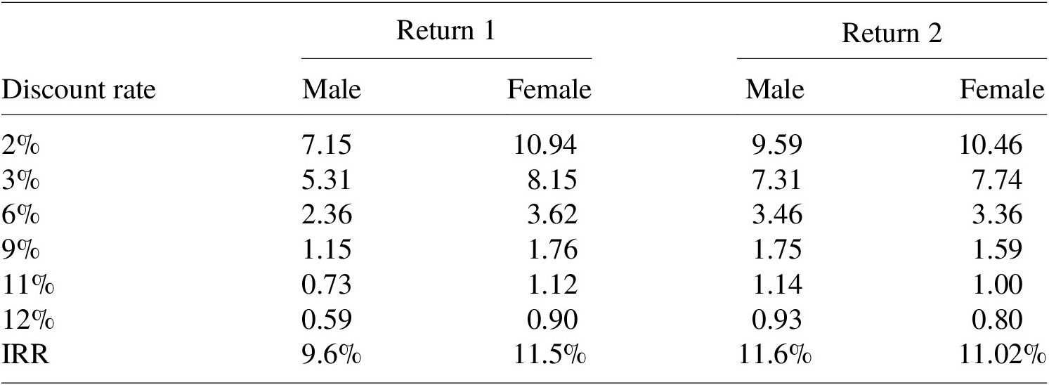
Exploiting the data available in Gertler et al. (Reference Gertler, Heckman, Pinto, Zanolini, Vermeerch and Walker2014, Reference Gertler, Heckman, Pinto, Chang, Grantham-McGregor, Vermeersch and Wright2021), we also estimate differences in the IRR by gender, considering school costs as in Table 2. Taking Returns 1 and 2 as the benchmark, we calculate the IRR for males, considering that the program impact on earnings by the age of 31 was ~27% (and 8% thereafter) for Return 1.Footnote 7 For Return 2, we considered all types of jobs return until participants were 31 years old, implying a 55% impact on wages (followed by the same 8% thereafter).Footnote 8 For females, the wage premium is 40% and 34% for Returns 1 and 2, respectively, and is subsequently estimated to be ~70% (Gertler et al., Reference Gertler, Heckman, Pinto, Chang, Grantham-McGregor, Vermeersch and Wright2021).Footnote 9 Table 5 presents the estimated IRR for each return by gender.
Benefit–cost ratio and IRR by gender

Table 5. Long description
Return 1: male BC ratio falls from 7.15 (2%) to 0.59 (12%), IRR 9.6%; female BC ratio falls from 10.94 to 0.90, IRR 11.5%. Return 2: male BC ratio falls from 9.59 to 0.93, IRR 11.6%; female BC ratio falls from 10.46 to 0.80, IRR 11.02%. Women’s IRR exceeds men’s in both returns, most markedly at low discount rates.
Under the Return 1 assumptions, men’s average estimate yields an IRR of 9.6%, while women’s is 1.9 percentage points higher (11.5%). This is not consistent with the gender differential in the IRR found in García et al. (Reference García, Heckman, Ermini Leaf and Prados2020) for the Abecedarian program, where returns are higher for men. In the Abecedarian US sample, the gender differential is driven by the stronger health effects for men, who experience considerably more positive outcomes – especially in cardiovascular and metabolic conditions compared to women – as well as substantially larger effects on savings related to avoided criminal behavior. However, our estimates include neither the impacts of the Jamaica Home Visiting program on health nor crime.Footnote 10
6. Conclusion
In summary, our method yields an IRR of 10.4–10.7% for the Jamaican early childhood stimulation intervention, based on the labor market benefits reported in Gertler et al. (Reference Gertler, Heckman, Pinto, Zanolini, Vermeerch and Walker2014, Reference Gertler, Heckman, Pinto, Chang, Grantham-McGregor, Vermeersch and Wright2021), the cost estimates in Zhou et al. (Reference Zhou, Heckman, Liu, Lu, Chang and Grantham-McGregor2023) and our own calculations and assumptions. After conducting various sensitivity analyses – considering different samples used for the analysis, varying ages of labor force entry and exit, and different discount rates – we conclude that our estimated IRR is robust. Under a range of plausible assumptions, the internal rate of return of the program is estimated to fall between 7.4% and 11.7% on average, with higher returns for girls. These estimates demonstrate the social profitability of the Jamaica Home Visit Program.
Despite its simplicity and robustness, the analysis in this article has several limitations that should be addressed in further research. Relying on metadata from previous studies (rather than original micro-data) limits our ability to estimate confidence intervals for the IRR. In addition, not forecasting other life-cycle benefits likely leads to an underestimation of the IRR, since – due to data limitations – we do not account for nonmonetary benefits such as improvements in health, reductions in crime and broader social effects.
Given the high levels of crime in Jamaica and the evidence from the Perry program in the United States – where most program gains stem from reduced crime among males – it is likely that we are underestimating the true IRR. Moreover, the program was targeted to a disadvantaged population in Kingston, Jamaica. Generalizing these findings to other populations will require additional longitudinal studies of ECD interventions that follow children into adulthood.
Appendix A: Details on inputs used to adjust from Zhou et al. (Reference Zhou, Heckman, Liu, Lu, Chang and Grantham-McGregor2023) to 2017 USD
Exchange rate and Consumer Price Index (CPI) evolution

Table A1. Long description
JM$/USD exchange rate: $116.97 (2015), $127.96 (2017, +9% vs. 2015), $153.43 (2022, +31% vs. 2015). US CPI (2010 = 100): 108.7, 112.4 (+3%), 134.2 (+23%). Jamaican CPI (2010 = 100): 141.1, 150.8 (+7%), 199.7 (+42%). Source: World Bank Data.
Source: World Bank Data.
Appendix B: Benefit–Cost ratios: US programs compared with Jamaica
The following table (Table B1) is an adaptation and update of Table 4.4 of Karoly, Kilburn and Cannon (Reference Karoly, Kilburn and Cannon2005) that presents the benefit–cost analysis of a variety of US ECD programs.
Benefit–cost ratios compilation from existing literature

Table B1. Long description
CCDP (Aos et al., 2004, combined, age 5, no ratio reported); HIPPY USA (Aos et al., 2004, home visiting/parent education, age 6, ratio 1.8); IHDP (Aos et al., 2004, combined, age 8, no ratio); NFP higher-risk sample (Karoly et al., 1998, home visiting/parent education, age 15, ratio 5.7); NFP lower-risk sample (Karoly et al., 1998, age 15, ratio 1.26); NFP full sample (Aos et al., 2004, age 15, ratio 2.88); Abecedarian (Masse and Barnett 2002, combined, age 21, ratio 3.23); Chicago CPC (Reynolds et al., 2002, combined, age 21, ratio 7.14); Perry Preschool excluding crime costs (Karoly et al., 1998, combined, age 27, ratio 5.15); Perry Preschool including crime costs (Barnett, 1993; Schweinhart, Barnes & Weikart, 1993, age 27, ratio 8.74); Perry preschool age 40 (Belfield, Barnett, Nores & Schweinhart, 2006, age 40, ratio 12.09); Perry Preschool age 40 (Heckman et al., 2010, age 40, ratio 6.8); ABC/CARE (García et al., 2020, combined, age 30, ratio 7.9); Perry age 40 (García et al., 2021, combined, age 40, ratio 9); Reach Up – the Jamaica program studied in this paper (home visiting, ages 25 and 31, ratio 13).
Note: Author’s compilation adapted from Karoly, Kilburn and Cannon (Reference Karoly, Kilburn and Cannon2005), but including more recent studies. Programs without b/c ratio estimation are due to negative or null benefits (see Karoly, Kilburn and Cannon (Reference Karoly, Kilburn and Cannon2005) for more detailed information). Karoly, Kilburn and Cannon (Reference Karoly, Kilburn and Cannon2005) summarized the literature from several interventions: for example, they revise work from Aos et al. (2004) who conducted a benefit–cost analysis for the Home Instruction Program for Preschool Youngsters, for the Nurse Family Partnership program. Aos et al. (Reference Aos, Lieb, Mayfield, Miller and Pennucci2004) also conducted benefit–cost ratio analysis for the Comprehensive Child Development Program (CCD) and the Infant Health and Development Program. They also include the analysis of CARE Abecedarian Program (Masse and Barnett, Reference Masse and Barnett2002), the Chicago CPC program Reynolds et al. (Reference Reynolds, Temple, Robertson and Mann2002) and several studies for the Perry Preschool Program, conducted by Karoly et al. (Reference Karoly, Greenwood, Everingham, Houbé, Kilburn, Rydell, Sanders and Chiesa1998), Barnett (Reference Barnett1993), Schweinhart, Barnes and Weikart (Reference Schweinhart, Barnes and Weikart1993) and the age-40 follow-up, by Belfield et al, (Reference Belfield, Nores, Barnett and Schweinhart2006). For our analysis, we also include three updated studies, two for the Perry Preschool Program (Heckman et al., Reference Heckman, Hyeok Moon, Pinto, Savelyev and Yavitz2010; García et al., Reference García, Bennhoff, Leaf and Heckman2021) and one for a pair closely related programs implemented in North Carolina: The Carolina Abecedarian Project (ABC), and the Carolina Approach Responsive Education (CARE), conducted by García et al. (Reference García, Heckman, Ermini Leaf and Prados2020). BC ratio based only on earnings for the two most influential studies are 4.25 for Perry (age 40) based on Table 9 from Belfield et al. (Reference Belfield, Nores, Barnett and Schweinhart2006) and 3 for the Abecedarian (García et al., Reference García, Bennhoff, Leaf and Heckman2021).
Appendix C: Construction of main wage estimates of the paper
Based on Gertler et al. (Reference Gertler, Heckman, Pinto, Zanolini, Vermeerch and Walker2014, Reference Gertler, Heckman, Pinto, Chang, Grantham-McGregor, Vermeersch and Wright2021), we construct four alternative returns that we present in Tables 2 and 3 of the main text.
Return 1 assumes a constant 24.6% earnings impact (constructed from Gertler et al., Reference Gertler, Heckman, Pinto, Zanolini, Vermeerch and Walker2014 as explained below) up to age 31 years followed by a 37% constant impact thereafter (based on Gertler et al., Reference Gertler, Heckman, Pinto, Chang, Grantham-McGregor, Vermeersch and Wright2021).
From Table 1, row 1, column 2 in Gertler et al. (Reference Gertler, Heckman, Pinto, Zanolini, Vermeerch and Walker2014) pasted below as Figure C1, we use the estimated treatment effect of 0.22 for full-time jobs. Since coefficients are expressed in log earnings, we take a log transformation to obtain the appropriate percentage impact on earnings as follows:

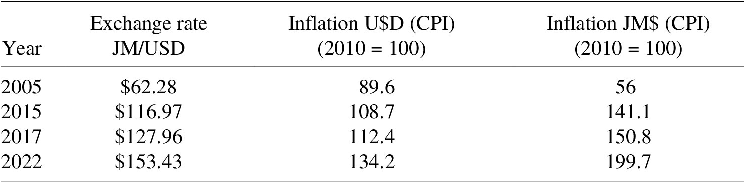
As stated above, the Return 1 specification assumes that the treatment and control groups remain constant until age 31. For computing the yearly incomes until age 31 for both groups, we use the control mean of 9.59 reported in Table 1 from Gertler et al. (Reference Gertler, Heckman, Pinto, Zanolini, Vermeerch and Walker2014) (row 4, column 2). Since 9.59 is expressed in log monthly earnings in 2005 Jamaican dollars, we need to update this value using the variation of Jamaica CPI and the JM$/US$ exchange rate. We constructed Table C1 using World Bank data to clarify our calculations.
Table 1 from Gertler et al. (Reference Gertler, Heckman, Pinto, Zanolini, Vermeerch and Walker2014).
Source: Gertler et al. (Reference Gertler, Heckman, Pinto, Zanolini, Vermeerch and Walker2014)

Figure C1. Long description
Reproduced table reports treatment effects on average log earnings at age 22. All job types: effect 0.30 (single p = 0.01, stepdown p = 0.02), control mean 9.40, N = 109. Full-time job: effect 0.22 (p = 0.04/0.04), control mean 9.59, N = 105. Non-temporary job: effect 0.39 (p = 0.01/0.02), control mean 9.67, N = 82. Combined rank mean: effect 0.09 (p = 0.04), N = 109. Statistically significant results shown in bold. Source: Gertler et al. (2014).
Jamaican and US CPI and exchange rate (2005–2022)

Table C1. Long description
JM$/USD exchange rate: $62.28 (2005), $116.97 (2015), $127.96 (2017), $153.43 (2022). US CPI (2010 = 100): 89.6, 108.7, 112.4, 134.2. Jamaican CPI (2010 = 100): 56, 141.1, 150.8, 199.7. Source: authors’ elaboration based on World Bank data.
Source: authors elaboration based on World Bank data.
We expressed the 9.59 control mean reported in Gertler et al. (Reference Gertler, Heckman, Pinto, Zanolini, Vermeerch and Walker2014) as US$ 2017 as follows:
-
1. First, we take an inverse log transformation on the reported control mean of 9.59 to express it in 2005 Jamaican dollars:

-
2. Then we update the earnings value using Jamaican inflation estimated as

Multiplying the value obtained in step 1 by the inflation (
$ {\pi^{JM}}_{2005-2017} $
 ), we obtain control mean earnings expressed in 2017 Jamaican dollars

-
3. Finally, to express the control mean earnings in US$ 2017, we use the value obtained in step 2 and the 2017 JM$/US$ exchange rate

-
4. Once we have the estimated control mean earnings in US$ 2017 (obtained in step 3), we can estimate the treatment mean earnings by multiplying the control mean earnings by the percentage change of 24.6% calculated before.

Now, the difference implies a
$ \mathrm{US}{\$}_{2017} $
 75.70 impact per month for the treatment group until age 31 (
$ \mathrm{US}{\$}_{2017}908.4 $
 per year).
Then, for ages 31 and above, we use Gertler et al. (Reference Gertler, Heckman, Pinto, Chang, Grantham-McGregor, Vermeersch and Wright2021) estimates. Specifically, for return 1, we used the effect size reported in Table 1, row 2, column 5 (0.37). Now, taking this value, we replicate the procedure done for the initial segment of the income stream. The only step we do not replicate in this case is the log transformation of the coefficient, since we take the 37% as the percentage change.
Our first step, in this case, is to take an inverse log transformation of the reported control mean (not the coefficient) in Table 1, row 2, column 3 of Gertler et al. (Reference Gertler, Heckman, Pinto, Chang, Grantham-McGregor, Vermeersch and Wright2021) to transform the monthly log earnings into monthly earnings in 2015 US dollars (as specified in Gertler et al., Reference Gertler, Heckman, Pinto, Chang, Grantham-McGregor, Vermeersch and Wright2021).

-
1. In this case, first we will transform the US$ 2015 to JM$ 2015 using the 2015 exchange rate (116.97 JM$/US$ according to World Bank data).

-
2. Next, we update this value using the Jamaican CPI between 2015 and 2017. That yields an inflation of 6.87%

-
3. Finally, we recover the 2017 US dollar value using the 2017 JM$/US$ exchange rate.

-
4. Once we have the estimated control mean earnings in 2017 US dollars (obtained in step 4), we can estimate the treatment mean earnings by multiplying the control mean earnings by the percentage change of 37% reported in Table 1 of Gertler et al. (Reference Gertler, Heckman, Pinto, Chang, Grantham-McGregor, Vermeersch and Wright2021) (see Figure C2).

Now, the difference implies a
$ \mathrm{US}{\$}_{2017}134.62 $
 impact per month for the treatment group for ages 31 and above (
$ \mathrm{US}{\$}_{2017}\mathrm{1,615} $
 per year).
Table 1 of Gertler et al. (Reference Gertler, Heckman, Pinto, Chang, Grantham-McGregor, Vermeersch and Wright2021).

Figure C2. Long description
Reproduced table reports treatment effects on log daily wage, log monthly earnings, and a rank-mean index for the full sample, non-migrant sample, female sample, and male sample, with control means, percentage change, effect size, t-statistics, and asymptotic/permutation p-values. Full sample: log monthly earnings +39% (effect size 0.37, single p = 0.05). Female sample: log monthly earnings +71% (effect size 0.70, single p = 0.03), significant results in bold. Male sample: smaller, mostly non-significant effects. Source: Gertler et al. (Reference Gertler, Heckman, Pinto, Chang, Grantham-McGregor, Vermeersch and Wright2021).
Using these values, we constructed the following table to clarify the wages used to compute the income stream for each group (Table C2).
Control and treatment income in US$ 2017

Table C2. Long description
Before age 31 (Gertler et al. Reference Gertler, Heckman, Pinto, Zanolini, Vermeerch and Walker2014): control $307.63, treatment $383.33. From age 31 (Gertler et al. Reference Gertler, Heckman, Pinto, Chang, Grantham-McGregor, Vermeersch and Wright2021): control $363.83, treatment $498.45.
For alternative income streams specifications, we define the elasticity growth alternative as

Where
$ \eta $
 es the income-age elasticity defined as

Equations (C1) and (C2) refer to the calculation method of the income used to compute the benefits for income stream in row (f) of Table 4.
C.1. Calculation of CI of the wage treatment effects
For the calculation of confidence intervals based on Gertler et al. (Reference Gertler, Heckman, Pinto, Zanolini, Vermeerch and Walker2014, 2021), we use the sample size and p-value reported in Table 1 of Gertler et al. (Reference Gertler, Heckman, Pinto, Zanolini, Vermeerch and Walker2014) and the sample size, p-value and t-stat reported in Table 1 of Gertler et al. (Reference Gertler, Heckman, Pinto, Chang, Grantham-McGregor, Vermeersch and Wright2021).
For Gertler et al. (Reference Gertler, Heckman, Pinto, Zanolini, Vermeerch and Walker2014), we assume a one-tail t distribution and calculate the t-stat using the reported p-value (0.04) and the N-2 degrees of freedom (N = 105 based on the full time jobs sample size reported). Once we have the estimated t-stat (−1.768), we divide the reported treatment effect (TE = 0.22) by the absolute value of the t-stat to obtain the standard error (0.1244). With the SE, we estimate the margin error (ME) for a 90% confidence interval, multiplying the SE by the critical t-value corresponding to 90% confidence using the sample size (for the degrees of freedom N-2). Then, the confidence intervals become:

For Gertler et al. (Reference Gertler, Heckman, Pinto, Chang, Grantham-McGregor, Vermeersch and Wright2021) the procedure is the same, but we do not need to estimate the t-stat because it’s already reported in their Table 1. In Gertler et al. (Reference Gertler, Heckman, Pinto, Chang, Grantham-McGregor, Vermeersch and Wright2021), the reported p-value and t-stat correspond to a one-sided test with 95% confidence, which is equivalent to a two-sided 90% confidence interval for symmetric distributions.
Appendix D: Incorporating the schooling costs to the IRR estimation
An additional analysis consists of accounting for future schooling costs associated with the documented improvements in schooling trajectories. Gertler et al. (Reference Gertler, Heckman, Pinto, Chang, Grantham-McGregor, Vermeersch and Wright2021) found a treatment effect of 0.77 additional years of education for the whole sample (0.25 for men and 1.33 additional years for women). We therefore estimate the cost of an additional schooling year using the per-capita school expenditures reported by the Jamaican Ministry of Education, Skills, Youth and Information.
First, we obtained per capita schooling costs from the website of the Jamaican Ministry of Education, Skills, Youth and Information (MOEY). In order to assume a conservative scenario, we use an average between the minimum and maximum values reported by the MOEY. According to Gertler et al. (Reference Gertler, Heckman, Pinto, Chang, Grantham-McGregor, Vermeersch and Wright2021), the control mean of education years is 10.69 (Table 2, row 1, column 3) and the estimated treatment effect is 0.77 for the full sample (Table 2, row1, column 4). The 10.69 years of education of the control mean corresponds to high school, so we use the average (between the minimum and maximum values reported) high school funding per capita per year cost reported by the MOEY (JM$489,680).
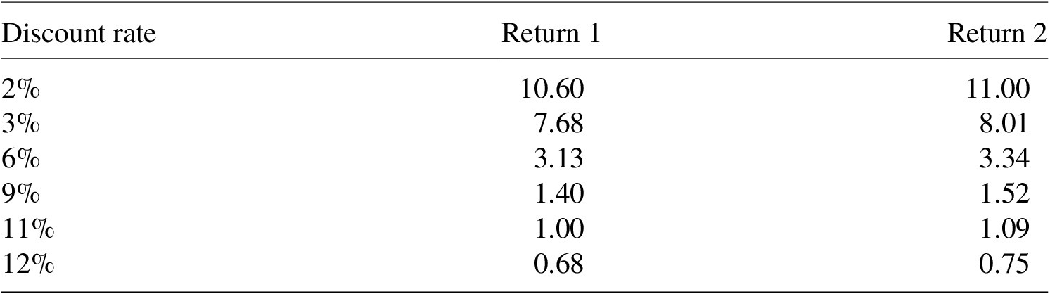
Since the reported per capita cost is in 2024 Jamaican dollars, we have to take it to US$ 2017 as we did with the benefits. First, we transform it into JM$ 2017 using the 2017 and 2024 Jamaican CPI reported by the World Bank data. This transformation yields a per capita cost of 2017 JM$ 329,365. Next, we transform it into US dollars using the 2017 JM$/US$ exchange rate as before (US$ 2,445). We also adjust this value using the variation of the GDP per capita in 2021 constant PPP dollars between 2000 and 2024 (17.3% increase); this yields an annual per capita cost of US$ 2,085. Finally, to compute schooling costs based on the program’s treatment effect on years of schooling, we adjust the US$2,085 by multiplying it by the reported treatment effect (0.77), which corresponds to the additional years of schooling attributable to the program. This yields a cost of US$1,605 per child. We incorporate this cost (as a negative flow) in the 16th year of the income stream (elementary school in Jamaica is mandatory starting at 5 years old, and adding 10.69 + 0.77 years will mean higher educational costs from age 16). Final estimates yield an adjusted IRR of 10.37% for return 1 and 10.74% for return 2. Table 1 presents the adjusted (and much lower) BC ratio estimates.
Adjusted BC ratio estimates including schooling costs

Table D1. Long description
BC ratio falls from 10.60 (Return 1) and 11.00 (Return 2) at a 2% discount rate to 0.68 and 0.75 at 12%. Adjusted IRR: 10.37% (Return 1), 10.74% (Return 2).






 Open access

