Implication
The prototype of a multi-Kinect system is presented that captures 3D data of dairy cows in motion for health monitoring. When fully developed, it will provide an inexpensive means of automated early lameness detection and livestock monitoring, thereby helping to increase animal welfare. The large amount of recorded data will provide a solid basis for scientific analyses and can help to deepen the understanding of connections between traits and genetics. Object recognition and methods to analyze the animals’ surfaces from the 3D data are important developmental steps that are approached using the wavelet transform.
Introduction
Several camera-based studies were conducted over the last years yielding high rates of correct classification in lameness detection in dairy cows. Song et al. (Reference Song, Leroy, Vranken, Maertens, Sonck and Berckmans2008), Pluk et al. (Reference Pluk, Bahr, Poursaberi, Maertens, Van Nuffel and Berckmanns2012) and Viazzi et al. (Reference Viazzi, Bahr, Schlageter-Tello, Van Hertem, Romanini, Pluk, Halachmi, Lokhorst and Berckmans2013) used digital 2D cameras to record walking cows from the side at distances of 3 to 6 m and analyzed step overlap, fetlock joints’ angles or back posture. There were also several camera-based studies dealing with body condition score (BCS) determination. Azzaro et al. (Reference Azzaro, Caccamo, Ferguson, Battiato, Farinella, Guarnera, Puglisi, Petriglieri and Licitra2011) used linear and polynomial kernel principal analysis to reconstruct cows’ shapes. Bercovich et al. (Reference Bercovich, Edan, Alcahantis, Moallem, Parmet, Honig, Maltz, Antler and Halachmi2012) presented BCS-prediction models that were based on five anatomical points. In both studies the animals were observed from a top view position using 2D cameras. The definition of ‘image background’ is complicated by changes in scenery and light when using 2D cameras for image acquisition according to Van Hertem et al. (Reference Van Hertem, Alchanatis, Antler, Maltz, Halachmi, Schlageter-Tello, Lokhorst, Viazzi, Romanini, Pluk, Bahr and Berckmans2013). Therefore, Halachmi et al. (Reference Halachmi, Klopcic, Polak, Roberts and Bewley2013) conducted tests with thermal images acquired from the animals’ backs. They estimated the BCS by fitting parabolae to the cows’ shapes fully automated. Another means of overcoming problems with image segmentation are 3D cameras. The distinction between image back- and foreground is easier because the relative distances of all pixel from the camera are known. Images of dairy cows’ rear views were captured for BCS estimation in Krukowski (Reference Krukowski2009) with a hand held Time-Of-Flight (TOF) 3D camera while the animals stood still. Additionally, an automated system for backfat thickness (BFT) determination based on a TOF camera mounted in top view position was presented in Salau et al. (Reference Salau, Haas, Junge, Bauer, Harms and Bieletzki2014, 1) and Weber et al. (Reference Weber, Salau, Haas, Junge, Bauer, Harms, Suhr, Schönrock, Rothfuß, Bieletzki and Thaller2014). The BFT was estimated reaching 0.96 correlation between the backfat thickness measured with a diagnostic ultrasound device and the estimator. TOF cameras measure ‘depth’ by calculating the phase shift between emitted infrared light and its reflection. As the phase shifts of several light signals were summed up to gather one measurement, the depth values were prone to motion artifacts (Hansard et al., Reference Hansard, Lee, Choi and Horaud2012). Additionally, large differences in depth measurements depending on the fur color occurred (Salau et al., Reference Salau, Bauer, Haas, Thaller, Harms and Junge2015). Viazzi et al. (Reference Viazzi, Bahr, Van Hertem, Schlageter-Tello, Romanini, Halachmi, Lokhorst and Berckmans2014) compared the Microsoft KinectFootnote 1 3D camera mounted in top view position to a 2D camera in side view position with regard to their applicability in lameness detection. Afterwards, the algorithms were improved and the classification results were optimized in Van Hertem et al. (Reference Van Hertem, Viazzi, Steensels, Maltz, Antler, Alchanatis, Schlageter-Tello, Lokhorst, Romanini, Bahr, Berckmans and Halachmi2014). The Kinect uses the measurement principle ‘Structured Light’ (Andersen et al., Reference Andersen, Jensen, Lisouski, Mortensen, Hansen, Gregersen and Ahrent2012). Distances between camera and objects are calculated from deformations in a predefined infrared pattern projected onto the scenery. Since depth values are determined from single signals, motion artifacts are no longer a problem. But the Kinect camera has technical difficulties, as well. No depth value can be calculated between the light dots of the infrared pattern projected by the Kinect camera, which leads to a coarser depth resolution with increasing distance from the camera (Andersen et al., Reference Andersen, Jensen, Lisouski, Mortensen, Hansen, Gregersen and Ahrent2012). Furthermore, Hansard et al. (Reference Hansard, Lee, Choi and Horaud2012) stated, that material properties strongly correlate to depth accuracy, and that both depth measurement principles had difficulties with various surfaces. The next generation of the Microsoft Kinect depth sensor is a TOF camera with significantly improved sensor and higher resolution (Lau, Reference Lau2013). It has not been available for data collection in this study.
Livestock holders require a low-cost system that allows simultaneous and reliable monitoring of multiple parameters and easily fits into existing barn passages. The latter implying that installations with a distance of several meters between cow and camera are inapplicable for the majority of dairy farms. The focus of the aforementioned studies was either on body condition or lameness. Currently, a system aiming to be applicable for both monitoring purposes and comprising six Microsoft Kinect cameras is being developed by the credited institutions. Important feasibility steps have been handled and the applicability for the desired monitoring purposes has been shown in Salau et al. (Reference Salau, Haas, Junge, Bauer, Harms and Bieletzki2014, 2). The process of partitioning an image into regions according to predefined characterizing properties is called segmentation. In Salau et al. (Reference Salau, Haas, Junge, Bauer, Harms and Bieletzki2014, 2) first steps to segment the Kinect recordings with respect to the image region containing the moving object captured by the system referred to as foreground and the standstill scenery referred to as background were presented. Object recognition and surface analysis are important next work items. The human ability to visually capture a scenery and distinguish between a multitude of objects is adjustable to translations, rotations and variations in shape and scale. For camera-based systems this object recognition, that is identifying a specific object in an image, is still a difficult and time consuming task. The depth value-based segmentation used in Salau et al. (Reference Salau, Haas, Junge, Bauer, Harms and Bieletzki2014, 2) is to be refined, and the object ‘cow‘ should be reliably recognized and distinguished from ‘non cow‘ objects like persons. With this objective, this study presents wavelet-based classifiers. Different computer configurations were compared regarding the wavelet analysis. The Kinect delivers depth information on the animal’s surface. As it is intended to use the system for monitoring later on, analysis of recorded surfaces, that is curvature changes or deformations, is a promising way to gather information on the animals. The present study evaluates wavelet analysis as a tool for such surface analysis.
Material and methods
Microsoft Kinect, hardware and recording
The Microsoft Kinect camera is a combination of an RGB camera and a depth sensor. The first acquires color images, the latter depth-data using the ‘Structured Light’ principle of measurement, where an infrared emitter projects a pattern of laser points whose deformation is detected by the infrared sensor and used to compute depth values. The Kinect camera has a 57° horizontal field of view (FOV) and 43° vertical FOV. The depth images have a maximal resolution of 640×480 pixel and can be acquired at up to 30 frames/s. The six cameras were simultaneously recording depth images that were stored in binary video streams. Interferences can occur in this setting, because the Kinect cameras detect overlapping patterns of other cameras which can lead to erroneous depth measurements as addressed in paragraph Prototype. For Kinect cameras to be recognized individually by a single computer, each camera needs to be connected to its own USB controller. When multiple cameras are used, simultaneous recording and data saving, synchronization of cameras and data assembling need to be handled. Alpha software for recording was developed based on the ‘SimpleViewer’ example from the OpenNI-projectFootnote 2 (OpenNI, 2013) since no suitable and readily available software could be found (Salau et al., Reference Salau, Haas, Junge, Bauer, Harms and Bieletzki2014, 2). A computer with an AMD FX-8350 CPU clocked at 4.0 GHz on an ASUS M5A99FX PRO R2.0 mainboard and Kingston Value RAM ECC-DDR3 clocked at 1.6 GHz (PC3-12800) was equipped with USB cards to accommodate six Kinect cameras. The six binary streams were stored in pairs on three 2 TB hard disks allowing 7.5 h of continuous recording of depth data. All calculations concerning the wavelet transforms as well as verification of the classifiers’ results were carried out on an AMD Phenom II X6 1100 T with 3.3 GHz and 16 GB RAM. The computational times of the wavelet transforms were calculated for the computer equipped and used for recording (4.0 GHz), because a real time application including the wavelet transforms is aspired. Additionally, they were calculated for the computer used later on for the calculations performed on recorded sequences (3.3 GHz).
Prototype
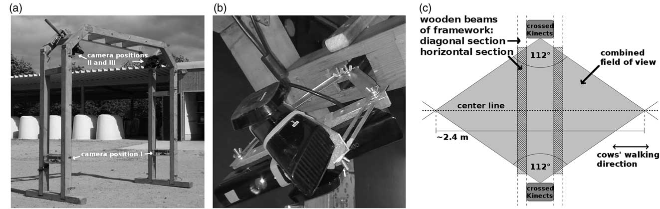
The prototype comprised the wooden framework shown in Figure 1a. Its total height was 2.18 m and its total width 2.25 m. The passage height was 2.08 m and the passage width 2.05 m. It had two connected arcs that were 0.32 m apart to leave room for cameras and cables and stood on two wooden beams. The two sides of the frame were each equipped with three Kinect cameras. One of them was mounted ~0.6 m above ground facing inwards with line-of-sight (LOS) parallel to the ground. As a protection from dirt and moisture, it was installed in a casing made of transparent acrylic glass that was not causing any loss in depth measurement accuracy. This side view camera was directly facing its counterpart on the other side but when a cow passed the infrared pattern of the opposite camera was occluded by the animal. Therefore, interferences were prevented. The remaining two cameras were mounted about 1.95 m above ground with a metal mounting bracket in the diagonal corner parts of the frame. They were attached to the bracket in a crossed fashion top-to-top with an angle of ~56° between their fronts (Figure 1b). This resulted in a combined horizontal FOV of 112° including an overlap of 2°, so that interferences occurred only in a negligibly fraction. The cameras were facing towards the floor at an angle of 45° in diagonal top view position so that the whole area between a cow’s back and its claws was in the FOV. The combined horizontal FOVs of all four top view cameras from both sides intersected in a rhombus with a center line of roughly 2.40 m (Figure 1c), allowing the acquisition of image sequences that show complete animals for three to five steps. As it was the case with the side view cameras, any occurring interferences between the top view cameras from opposite sides of the system were prevented when an animal walked through the framework, as it occluded the infrared pattern from the opposite cameras view.
Prototype. A frame made of wood was constructed and six Kinect cameras were mounted (a). Each side was equipped with three cameras. One of those was mounted horizontally about 0.6 m above ground facing inwards (position of camera I). The other two were fixated top-to-top (b), with an angle of ~56° between them, in the diagonal corners of the frame (position of cameras II and III), facing the passing animals in diagonal top view. A schematic representation of the recording’s setting (c) illustrates their combined horizontal field of view (FOV): The FOV (112° from both sides) overlapped in a rhombus with ≈2.4 m diagonal. The multi-Kinect-system observed several steps of cows walking on the center line (dotted).

Data collection
Data sets for developmental purposes used in this feasibility study were recorded at the cattle show ‘Neumünster am Abend’ (23 January 2014). It took place at Neumünster, Germany, and was organized by Rinderzucht Schleswig-Holstein eG. Cows were guided through the framework once led in halter when they were recorded. Arbitrary recordings of only Holstein–Friesian cows were chosen for analyses. The identities of the animals were irrelevant in this study, as not the distinction between individuals was aspired, but the system should be trained to recognize cows.
Three image sequences recorded by a sideview camera and three image sequences recorded by a topview camera were chosen from this development data set. All six sequences showed a person leading a cow by rope. In total three Holstein–Friesian cows were involved corresponding to three pairs of related sideview and topview sequences. The number of images gathered per cow/person was not constant, as the walking speed differed. The sequences were chosen to start two images before and end two images after cow or leading person were captured by the cameras. All images in between were considered for analysis. As an exception, the images showing both a cow and a person are excluded from the classification whether a pixel is located on a cow’s or a person’s surface (compare paragraph Classifiers). The sequences recorded by topview cameras showed person and cow diagonally from above. Depending on how far cow or person have walked through the framework, the person’s torso and the cow’s head, back, pelvis, tail or udder from behind could be seen. The sequences recorded by sideview cameras showed the person’s legs and the cow’s legs, udder and lower rump, again depending on cow’s or person’s relative position to the framework. In Supplementary Material S1 an example video footage is provided. Two sideview and two topview sequences were declared learning sequences. The remaining two (one sideview and one topview sequence) were used as test sequences later on. All sequences had been segmented into fore- and background in advance (Salau et al., Reference Salau, Haas, Junge, Bauer, Harms and Bieletzki2014, 2). The results had been visually checked and refined. Furthermore, digital lists which images in the sequences showed a cow or a person, respectively, had been compiled by visual inspection.
Wavelet transform applied to Kinect recordings and calculated criteria
This study focusses on the application of two-dimensional wavelet transform to data recorded with the Microsoft Kinect. The theoretical details on the method of wavelet analysis are described in Supplementary Material S2 or could be found in literature (Daubechies, Reference Daubechies1990; Louis et al., Reference Louis, Maaß and Rieder1998; Bergh et al., Reference Bergh, Ekstedt and Lindberg2007).
A goal was to provide wavelet-based classifiers to support foreground definition and object recognition. For this purpose, the wavelet that fits the given data best and an appropriate decomposition level had to be specified. Four differently shaped wavelets were chosen (Figure S2.2 in Supplementary Material S2): the haar wavelet, Daubechies No.2 (db2), the Symlet wavelet No.3 (sym3) and the biorthogonal 1.5 wavelet (bior1.5). The functions wavedec2.m and wrcoef2.m (MATLAB, Inc. The MathWorks, 2007a; Wavelet Toolbox, Misiti et al., 2014) were applied. To compare how well the wavelets fitted the given type of data, wavelet transforms up to the maximally possible decomposition level given the size of the image (MATLAB function wmaxlev.m) were performed. An approximation of the original image was calculated using these results (Supplementary Material S2, Equation S2.2). The squared pixelwise differences between original and the approximated signal were calculated and their maximal value (MS: Maximum of Squares) as well as their sum (SS: Sum of Squares) were determined. For the haar and the bior1.5 wavelets a mean computational time per image was determined on 644 images chosen from sideview and topview sequences.
Application of the two-dimensional wavelet transform using one level of decomposition resulted in three matrices Dh, Dv and Dd per image holding the values of reconstructed details in horizontal, vertical and diagonal direction. The matrices were of the same size as the original image. Additionally, all absolute details were summed up: DAll:=|Dh|+|Dv|+|Dd|. Using the information, whether a pixel belongs to the image fore- or background (see paragraph Data collection), the absolute values of the details in Dh (respectively Dv, Dd and DAll) were for every image averaged within those image regions:
 $${\rm AvAbsDet}^{{\rm h}} ({\rm foregr}.)\,\colon\,{\equals}{{\sum_{{(i_{x} ,i_{y} )}} \left| {{\rm D}^{h} (i_{x} {\rm ,}i_{y} )} \right|} \over {{\rm No}.(i_{x} ,i_{y} )}},(i_{x} {\rm ,}i_{y} )\,\colon\,{\rm foreground}\,{\rm pixel}$$
 $${\rm AvAbsDet}^{{\rm h}} ({\rm backgr}{\rm .})\,\colon\,{\equals}{{\sum_{{(i_{x} ,i_{y} )}} \left| {{\rm D}^{h} (i_{x} ,i_{y} )} \right|} \over {{\rm No}{\rm .}(i_{x} ,i_{y} )}},(i_{x} {\rm ,}i_{y} )\,\colon\,{\rm background}\,{\rm pixel}$$
The Averaged Absolute Detail values (AvAbsDet) for the other types of details were named AvAbsDetv(fore/backgr.), AvAbsDetd(fore/backgr.), AvAbsDetAll(fore/backgr.). They were calculated according to equations (1) and (2). For all four types of details the AvAbsDet-values of the two learning sequences recorded by the sideview camera were fused to one data set for statistical analysis. The same was done with the values of the two learning sequences recorded by the topview camera. This resulted in vectors (AvAbsDeth/v/d/All(foregr.)img)img in sequence of averaged details from the images’ foreground and vectors (AvAbsDeth/v/d/All(backgr.)img)img in sequence of averaged details from the images’ background for sideview as well as topview sequences.
Additionally, the vectors (AvAbsDeth/v/d/All(foregr.)img)img in sequence of averaged foreground details were each split up into two subvectors according to the lists of images showing a person or a cow (see paragraph Data collection): (AvAbsDeth/v/d/All(foregr.)img)img shows COW and (AvAbsDeth/v/d/All(foregr.)img)img shows PERSON. This resulted in one vector of averaged details calculated from a person’s surface and one vector of averaged details calculated from a cow’s surface for both camera view points.
Classifiers
Two types of binary classifiers were implemented in MATLAB and applied to the test sequences. At first, the reconstructed details were used to distinguish between pixel belonging to the image fore- and background. At second, the details were used to decide whether a foreground pixel belongs to a cow’s or a person’s surface. For both classifier types four versions were implemented, each using a different type of details (Dh, Dv, Dd, DAll). From the learning sequences mean values for the background (mean(((AvAbsDet(backgr.)img)img)) and foreground details (mean((AvAbsDet(foregr.)img)img)) were calculated for Dh, Dv, Dd and DAll. Series of thresholds ranging from zero to mean(((AvAbsDet(backgr.)img)img) were used to perform pixelwise classifications between fore- and background. Similarly, thresholds ranging from zero to mean((AvAbsDet(foregr.)img)img) were used for the decision, if a pixel belongs to a cow’s or a person’s surface. This was done within both test sequences and for all four types of details.
The pixelwise decisions between fore- and background made by the wavelet-based classifier were compared to the former segmentation results via computer. Similarly, the lists which images in the test sequences showed a cow or a person (paragraph Data Collection) were used to check the wavelet-based classifications concerning a pixel’s location. Images showing a cow AND a person or none of them were not included in the evaluation of these classifications’ results.
For every used threshold the numbers of pixel classified as true positive (TP), true negative (TN), false positive (FP) and false negative (FN) were derived from the results of both types of classifiers. This led to pairs of values for sensitivity:=TP/(TP+FN) and specificity:=TN/(TN+FP) varying with the thresholds. Plotting the sensitivity values against 1-specificity values, gives a monotonously increasing curve, called Reciever Operation Characteristic (ROC) curve (Bradley, Reference Bradley1997). The Area Under ROC Curve (AUC) serves as a measure for the performance of binary classifiers. ROC curves were plotted for all classifiers, and AUC values were calculated.
Statistical methods
The Statistics Toolbox of MATLAB (Inc. The MathsWorks, 2007b) was used to perform all statistical calculations.
For all four wavelets and both camera viewpoints sample size, minimal and maximal value, mean and standard deviation for the AvAbsDet-values determined from the four learning sequences were calculated. QQ-plots were plotted and inspected visually to compare the quantiles of the data’s distribution against the quantiles of a normal distribution. A two-sample F-test was performed to check for variance homogeneity between fore- and background details. Equality of means in fore- and background details was tested with a parametric two-sample t-test. When homogeneity of variance could not be guaranteed, it is called the Behrens–Fisher problem (Dudewicz et al., Reference Dudewicz, Ma, Mai and Su2007), and the premises of the t-test do not hold. In those cases Welch’s t-test (Welch, Reference Welch1947) was performed to compare the means in fore- and background details. The Welsh’s t-test delivers an approximate solution to the Behrens–Fisher problem, by using a test statistic, which shows an approximate Student’s t-distribution under the null hypothesis. Its number of degrees of freedom was approximated by Satterthwaite’s formula (Allwood, Reference Allwood2008). Levels of significance as well as 95% confidence intervals were calculated. The effect size η 2=t 2/(t 2+dof) (t 2: test statistic, dof: degrees of freedom) was calculated, if a significant effect could be stated by the t-test.
For the averaged details of person’s surface and cow’s surface the same descriptive statistics and, in addition, the median were calculated. Median-test and Wilcoxon-rank-sum-test (Wilcoxon, Reference Wilcoxon1945) were performed on the averaged detail values grouped according to whether cow or person was in the image foreground. The level of significance was calculated while running the Wilcoxon-rank-sum-test. For the significant effects stated by the Wilcoxon-rank-sum-test the effect size η 2 was calculated by dividing the test statistic by the degrees of freedom.
For the comparisons between fore- and background as well as between person’s and cow’s surface boxplots were generated.
Results
Selecting wavelets and decomposition level
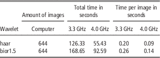
The measures of differences MS and SS (Materials and methods, Wavelet transform applied to Kinect recordings and calculated criteria) are given in Table 1 for all used wavelets. Beyond this point no more results for the db2 or sym3 wavelet are presented. As other aspects seemed more important to be illustrated for the readers’ understanding, no QQ-plots are displayed (examples of QQ-plots are provided in Supplementary Figures S1). Their inspection led to the insight that the AvAbsDet-values (equations (1), (2)) could be considered normally distributed for decomposition levels one and two, but the quantiles of the AvAbsDet-values diverged from the quantiles of the normal distribution when the decomposition level rose. Additionally, with higher decomposition levels the number of cases without significant differences between image fore- and background details increased. Therefore, further results’ presentation is limited to decomposition level 1. The computational times of the wavelet transforms are displayed in Table 2 in comparison between the two used computers (3.3 and 4.0 GHz). For the computer with 3.3 GHz, the mean computational time per image for the haar wavelet was only 77% of the time needed for the transformation of one image using the bior1.5 wavelet. For the faster computer the percentage even dropped to 64%.
Reconstruction errorsFootnote a for all four wavelets and for the sequences recorded in sideview and topview

a Depicted are the maximal value (MS: Maximum of Squares) and the sum (SS: Sum of Squares) of the squared pixelwise differences between reconstructed image and original image.
Computational times for the haar and the bior1.5 wavelet calculated on two separate computers (3.3 and 4.0 GHz) on 644 images chosen from sideview and topview sequences

Statistical results concerning the detail values
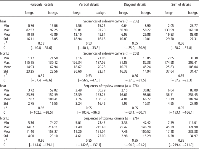
The sideview and topview sequences consisted of 208 and 276 images in total, respectively. Table 3 presents the descriptive statistics for the AvAbsDet-values calculated from decomposition level one. (The respective descriptive statistics calculated from decomposition level two can be found in Supplementary Table S1.) The differences between fore- and background means were significant for both wavelets and sideview as well as topview sequences. The effect sizes η 2 were high (η 2⩾0.5) for the sideview sequences and very high (η 2=0.95) for the topview sequences.
Descriptive statistics for the absolute values of horizontal, vertical, diagonal and summed details for every image averaged within image fore- and backgroundFootnote a

a Details were calculated from transformations with the haar and the bior1.5 wavelet at first decomposition level. The differences in means in image fore- and background were analyzed by performing a t-test. The significance levels were <0.001. Columns 2 and 3, 4 and 5, 6 and 7, and 8 and 9 belong to the horizontal, vertical, diagonal and summed details, whereas within each type of details the first column presents the descriptive statistics for the fore- and the second column presents the descriptive statistics for the background pixel. η 2 and CI denote effect sizes and boundaries of 95% confidence intervals, respectively. The table’s cells for η 2 and CI span across the two columns holding the values of the groups in comparison.
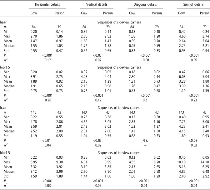
The sideview sequences contained 84 images showing a cow and 79 images showing a person. For the topview sequences there were 143 cow images and 43 person images. In Table 4 the descriptive statistics for the AvAbsDet-values are displayed in comparison between images with cows and persons. (The respective descriptive statistics calculated from decomposition level two can be found in Supplementary Table S2.) Except for the diagonal details calculated using the haar wavelet on the topview sequences the medians concerning the cows’ and the persons’ surfaces differed significantly. The effect sizes showed different behavior between wavelets in sideview sequences. Nearly disjoint ranges in η 2 could be observed, as η 2 varies between 0.02 and 0.17 for the haar wavelet and between 0.17 and 0.28 for the bior1.5 wavelet. The effects for the haar wavelet were small (η 2=0.02, vertical details), small to medium (η 2 between 0.07 and 0.09, diagonal and summed details) or medium (η 2⩾0.17, horizontal details) according to Cohen (Reference Cohen1988). The effect sizes with the bior1.5 wavelet were generally higher and indicated medium effects (η 2⩾0.17, vertical details), medium to large effects (η 2 between 0.2 and 0.23, diagonal and summed details), and large effects (η 2⩾0.28, horizontal details). It has to be noticed, that with both wavelets the smallest values for η 2 were observed for the vertical details and the largest η 2 values could be found for horizontal details. When it came to the effect sizes belonging to the topview sequences, the bior1.5 wavelet was no longer superior, as all effects were small (η 2 between 0.02 and 0.06).
Descriptive statistics for the averaged absolute values of horizontal, vertical, diagonal and summed details concerning the analysis of differences in cows’ and persons’ surfacesFootnote a

a Wavelet decompositions were calculated using haar and bior1.5 wavelet at first decomposition level. N.S. indicates no significant differences in medians. P and η 2 denote Wilcoxon-rank-sum tests’ significance levels and effect sizes.
In Supplementary Figure S2 examples of boxplots were provided.
Binary classifiers
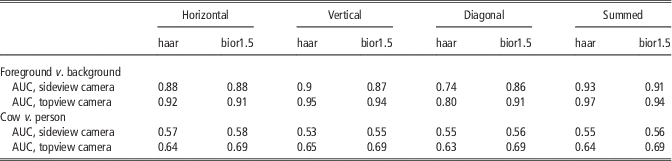
The binary classifiers’ evaluations by AUC values are given in Table 5.
Area under ROC curve (AUC) values for binary classifiers based on reconstructed wavelet detailsFootnote a

a The AUC values for classifiers that distinguish between image fore- or background and cows’ or persons’ surfaces are presented in the rows 1 to 5 and 6 to 10, respectively. Classifiers were based on horizontal details (columns 2, 3), vertical details (columns 4, 5), diagonal details (columns 6, 7) and the sum of all details (columns 8, 9) reconstructed from wavelet transforms using the haar and the bior1.5 wavelet with one level of decomposition. Classifiers were tested using sequences recorded from cameras in sideview (rows 4, 9) and topview (rows 5, 10).
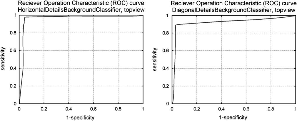
When it comes to distinguishing between fore- and background, the first thing to notice is, that the AUC values calculated from classifying the topview test sequence were higher than the AUC values from the sideview test sequence. Nearly all AUC values were ⩾0.86. The classifier based on transformation with the haar wavelet was superior to the classifier based on transformation with the bior1.5 wavelet. An exception were the diagonal details, where the classifier based on the haar wavelet showed considerably lower AUC values (0.74 in sideview, 0.8 in topview) than with the other types of details (⩾0.88 in sideview, ⩾0.92 in topview). The classifier based on the bior1.5 wavelet also had its lowest values (0.86 in sideview, 0.91 in topview) with the diagonal details, but the differences in comparison with horizontal and vertical details (0.87 and 0.88) in sideview are negligible. In topview the AUC value concerning the horizontal details even coincided with the diagonal details’ AUC value. The classifier based on the bior1.5 wavelet thus showed a more homogenous behavior in AUC values, whereas the haar wavelet-based classifier clearly had a weak spot when it came to diagonal details. Concerning both wavelets, the classifiers implemented using the sum of all details had the highest AUC values (0.93 and 0.93 in sideview, 0.97 and 0.94 in topview). Figure 2 exemplarily presents ROC curves for the haar wavelet-based classifier distinguishing between image fore- and background. Chosen were the illustrations of sensitivity and 1-specificity values evaluated from the topview test sequence and concerning the horizontal and the diagonal details. The ROC curves for the binary classifiers based on a transformation with the bior1.5 wavelet are comparable and their courses mirror the associated AUC values given in Table 5.
Reciever Operation Characteristic (ROC) curves for binary classifiers based on reconstructed wavelet details. The thresholds were equidistantly chosen between zero and mean(((AvAbsDet(backgr.)img)img). For this series sensitivity:=TP/(TP+FN) and specificity:=TN/(TN+FP) were calculated from the classifiers’ results, and the sensitivity values were plotted against the 1-specificity values. Exemplary ROC curves for the results of the classifiers used on the topview test sequence are presented. The classifiers were based on the horizontal and diagonal details calculated from wavelet transforms of one decomposition level using the haar wavelet.

The classifiers deciding whether a pixel belongs to a cow’s or a person’s surface, showed much smaller AUC values. For the sideview sequences, the highest values were found with the horizontal details (0.57 with the haar wavelet, 0.58 with the bior1.5 wavelet). The lowest AUC value was 0.53 (vertical details, haar wavelet) and all other AUC values were 0.55 (haar wavelet) or 0.56 (bior1.5 wavelet). They show a very uniform behavior, and the classifiers were only little superior to the random decision represented by AUC value 0.5. For the topview sequences, the classifiers performed more successfully. Concerning the haar wavelet the AUC values ranged from 0.63 (diagonal details) to 0.65 (vertical details). All AUC values for the bior1.5 wavelet-based classifier were 0.69.
Discussion
Selecting wavelets and decomposition level
The choice of a suitable wavelet is an important but not easy task. Several studies have been analyzing which wavelet was best used for a specific type of data (Megahed et al., Reference Megahed, Moussa, Elrefaie and Marghany2008; Mohd Tumari et al., Reference Mohd Tumari, Sudirman and Ahmad2013). But it has not been this study’s goal to find the most suitable wavelet for the analysis of Kinect recordings among the wide range of wavelet families provided by the MATLAB Wavelet Toolbox. With wavelet transform leading to promising results in these applications, a detailed specification could be carried out as future work. Therefore, the wavelets under comparison here were chosen with regard to preliminary considerations. According to Kiencke et al. (Reference Kiencke, Schwarz and Weickert2008), it is of advantage when the signals energy is preserved by the wavelet transform. This is guaranteed by using orthogonal wavelets (Farge, Reference Farge1992). Therefore, a selection of orthogonal (haar, db2, sym3) and a biorthogonal wavelet (bior1.5) were considered. The biorthogonal wavelets use differently shaped functions for decomposition and reconstruction (Supplementary Material S2, Figure S2.2). The functions used for decomposition and reconstruction are related by duality, that is they are not only both orthogonal wavelets but orthogonal to each other (Louis et al., Reference Louis, Maaß and Rieder1998; Bergh et al., Reference Bergh, Ekstedt and Lindberg2007). The haar wavelet was the same as db1 but differed from db2 in shape, had no sharp edges and it was the only not continuous wavelet chosen for the comparison. The Symlet sym3 differed from db2 in shape and in the number of oscillations. The comparison between these four wavelets is discussed below. It turned out, that the piecewise constant or smooth wavelet functions were chosen for further analysis (haar, bior1.5). Therefore, no higher order members of the Daubechies, Symlet and biorthogonal family or any member of the Coiflet family were analyzed, as they all strongly oscillate.
To specify the most suitable wavelet among the four wavelets in comparison, measures were introduced, how well they matched the given data. An approximation to the original image was constructed from the results of wavelet transforms to the maximal level. Comparing this approximated image to the original was a way to measure the loss of information caused by describing the data via the scaled and shifted wavelet and scaling function. All reconstruction errors were very small, but the values for db2 or sym3 wavelet exceeded the ones of the haar and the bior1.5 wavelet by six to eight decimal powers, concerning both MS and SS (Maximum and Sum of Squares, Materials and methods, Wavelet transform applied to Kinect recordings and calculated criteria). The haar wavelet often shows good reconstruction properties, because wavelet and scaling function were (piecewise) constant functions (Figure S2.2 in Supplementary Material S2). With constant functions most data can be approximated at least satisfactorily. The bior1.5 wavelet uses piecewise constant functions for reconstruction and corresponding rounded versions for decomposition. The db2 and sym3 wavelets and their scaling functions are roughly shaped compared to the bior1.5 wavelets and scaling functions. The depth values depend on the position of the pattern’s dots relative to each other (Lau, Reference Lau2013). They are thus not calculated from one spot, but little areas of the scenery illuminated by the infrared pattern. This might be a reason, why piecewise constant functions were more suitable to match the Kinect recordings than functions with sharp edges. The decision between the haar and the bior1.5 wavelet could not be made in conclusion. The reconstruction errors of haar and bior1.5 wavelet were similarly small and significant differences between image fore- and background details could be observed for both of them. On the one hand, the haar wavelet exhibited two cases concerning the first two decomposition levels (Table 4, Supplementary Table S2) where the effect of the species had not been significant, whereas considering the bior1.5 wavelet the medians differed significantly in any case. Also the AUC values of the bior1.5 wavelet-based classifiers (Table 5) concerning the decision whether a pixel is positioned on a cow’s or a person’s surface were larger than the haar wavelet-based classifiers’ AUC values. On the other hand, computational times should be kept small to make integration in a real time application possible, and the haar wavelet needed only 64% of the computational time. Additionally, the haar wavelet-based classifiers distinguishing between image fore- and background showed higher or equal AUC values for all types of details except the diagonal details. Since the AUC values calculated for the diagonal details were with both wavelets smaller than for the remaining types of details, in a future implementation this type of details is unlikely to be used. With horizontal, vertical or sum of details the haar wavelet-based classifier performed superior to the classifier based on the bior1.5 wavelet. The results gained from this study implicated, that the bior1.5 wavelet should be used on the recordings from the cameras in topview position. When it comes to the topview sequences, all classifiers relating to the image region performed very well and the AUC values for the bior1.5 wavelet-based classifiers to distinguish between species were higher than the corresponding AUC values for the haar wavelet. As for the sideview sequences the performances did show more homogeneous behavior, the haar wavelet should be used to save computational time. The practicability of both wavelets will have to be tested in the implementation of further methods.
Object recognition
An image region is a nonempty part of the image chosen according to a predefined property. In the present study the image regions foreground, which contained objects recorded while moving through the frame (Figure 1), and background, which contained the standstill scenery, were considered. Values of averaged absolute details were calculated from fore- as well as background for every image. It had been observed in advance, that the details’ values’ range per image was very wide. Significant differences in mean were to be expected, because in illustrations the values observed in the image background were so large, that the variation in detail values in the foreground could not be properly displayed (Figure S2.3 in Supplementary Material S2). For all types of details, the sizes of the image region’s effect were high. The Kinect camera’s accuracy in depth measurement decreases with increasing distance from the camera (Andersen et al., Reference Andersen, Jensen, Lisouski, Mortensen, Hansen, Gregersen and Ahrent2012), because the radii of the infrared pattern’s cones increase (Lau, Reference Lau2013). Additionally, a larger part of the scenery is presented by each pixel. The image therefore contains more noise in those regions. As the details’ values represent the high frequency parts in the image (Farge, Reference Farge1992; Kaur and Mehra, Reference Kaur and Mehra2010), they show higher values with increasing distance from the camera. This effect was even higher in topview sequences than in sideview sequences. Theoretically, the LOSs of the Kinect cameras in sideview position were parallel to the ground and the cameras could see further than the Kinect cameras in topview position, whose LOSs intersected with the ground. But the Kinect camera discarded all erroneous depth values, thus all values for pixel representing points too far away to deliver reliable depth measurement, were set to zero (Andersen et al., Reference Andersen, Jensen, Lisouski, Mortensen, Hansen, Gregersen and Ahrent2012; Lau, Reference Lau2013). For this reason, a part of the background did not have to be considered in the sideview recordings since the pixel values were invalid, whereas for the topview cameras a higher number of valid background pixel existed. This might be a reason, why differences in distances from the camera between passing cow and scenery behind the animal were thus more considerable in the topview than the sideview cameras’ LOSs. Additionally, the cows were passing the topview cameras with larger distance than the sideview cameras, because those were mounted in the upper part of the framework. This resulted in larger effects of the image region when it came to the cameras in topview position. There were two types of ‘image background’ concerning the sideview cameras in the presented prototype: At first, there were the opposite wooden beams of the framework and walls or objects in about the same distance from the camera (Material and methods, Prototype, Figure 1). At second, there were the floor areas within the passage. Parts of the floor were technically nearer to the camera than a passing cow. As part of the standstill scenery those are considered image background as well. Here, also, an increased noise level could be observed (Figure S2.3 in Supplementary Material S2). It has to be considered, that this part of the scenery could be seen not only by the Kinect camera itself but by the Kinect camera from the opposite side as well even when a cow walked through the passage (Figure 1 and S2.3 in Supplementary Material S2). The occurring interferences (Material and methods, Prototype) might be one reason for higher detail values. Another reason for a less accurate representation of the ground’s surface in comparison to the passing cow’s surface might be that the ground’s surface was parallel to the camera’s LOS. The infrared pattern hit the cow perpendicularly and produced clearly bounded dots on its surface, so depth values could be determined precisely. The ground was hit by the cones of the projected pattern in a very steep angle making the localization of the pattern’s dots and hereby the calculation of depth values difficult.
Concerning the recordings made from sideview position, the second type of image background complicated the segmentation based on comparison with an averaged image of the empty scenery or depth values. In Salau et al. (Reference Salau, Haas, Junge, Bauer, Harms and Bieletzki2014, 2) segmentation was achieved by averaging a predefined number of images of the scenery without any moving objects. Afterwards, the difference between every sequential image and this averaged background image was analyzed to specify the moving objects. In addition, Salau et al. (Reference Salau, Haas, Junge, Bauer, Harms and Bieletzki2014, 2) applied upper and lower thresholds for the distance from the camera, in order to lose pixel showing too high or too low depth values to belong to the image foreground. The considerable variation in floor areas often averaged to unreliable values. When an image was compared to this averaged background, the noise in the floor areas often exceeded the depth value differences caused by a moving object. Additionally, the floor areas showed similar depth values as the cows’ claws touching the ground. In previous attempts leftovers of floor areas in the segmented images had been the result. For reliable claw determination and gait analysis a refinement of these segmentation results was needed. Due to the wavelet transform’s properties to describe the high frequency parts in the image, the classifier to distinguish between image regions performed very well. An exception was the classifier based on the diagonal details calculated from the transform with the haar wavelet. A reason for this might be that the two-dimensional haar wavelet and scaling function were assembled from horizontal plane pieces whose edges are parallel to the image edges. The description of the diagonal components in the high frequency parts might be less exact.
With regard to all camera positions, the segmentation steps based on depth values and differences to an averaged background image came with the problem that they could not distinguish between cows and other objects that were moving and had a similar distance to the cameras. In modern cow barns with freely moving cows (Tucker et al., Reference Tucker, Weary and Fraser2004) it could not always be avoided, that also stable personnel is captured by camera-based monitoring systems. In addition, it would be time consuming and expensive, if animal holders had to view the recordings, in order to detect the cows before animal-related information could be computed. To widen the aspired system’s applicability as a full time monitoring solution, the possibility to automatically distinguish between cows and other objects had to be provided. Supplementary methods were needed to handle the decision about the recorded objects’ nature. Examples (Figure S2.3 in Supplementary Material S2) suggested, that the averaged absolute wavelet details could be used for this as well, because the details in the cow’s and the person’s region were displayed with different colors, indicating that the values differed. This could be expected, as fur and clothing or human skin exhibit different surface structures, and according to Hansard et al. (Reference Hansard, Lee, Choi and Horaud2012) depth measurement accuracy significantly depends on the material. Therefore, the details in the foreground regions were examined closer. As no influence was taken, which image showed a person or a cow, the numbers of cow and person images were unbalanced for the topview sequences. Therefore, the median seemed to be the more suitable measure of center. Apart from two exceptions both concerning the haar wavelet, all detail values’ medians differed significantly (Table 4). Regarding the sideview sequences, both wavelets showed the same ranking in detail types according to effect sizes η 2. The η 2 values concerning the haar wavelet covered a much wider relative range (0.02 to 0.2=10×0.02) than concerning the bior1.5 wavelet (0.15 to 0.31≈2×0.15). AUC values indicate, that most classifiers performed slightly better than a randomly made decision, that would correspond to AUC=0.5 (Fawcett, Reference Fawcett2006). For the topview sequences, the AUC values of the bior1.5 wavelet-based classifiers were clearly superior, but the effect sizes did not systematically exceed the effect sizes belonging to the haar wavelet’s details. For the haar wavelet the medians in details are larger for the cows’ surfaces than the persons’ surfaces. For the bior1.5 wavelet the medians were larger for cows regarding sideview recordings and larger for persons regarding topview recordings. An explanation for these remarkable medians might be found in further analyses regarding the combination of the bior1.5 wavelet’s characteristics and the perspective from diagonal topview position. The largest effects on details’ medians related to the sideview sequences and both wavelets corresponded to the highest AUC values for the concerning binary classifiers. Apart from that, the AUC values did not mirror the effect sizes. Since variance inhomogeneities (Material and methods, Statistical methods) indicate differences in the variation on the surfaces of the recorded objects, classification results might in future work be improvable by using the details’ variances as additional decision criterion.
A possibility for wavelet transform’s application in surface analysis
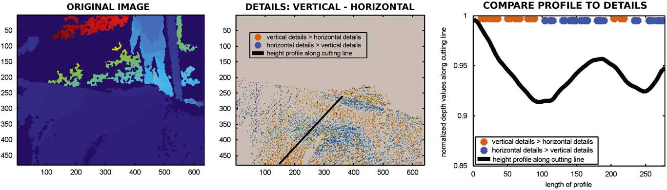
Apart from the object recognition application presented in this study, wavelet transforms were used in the definition of feature point detectors and descriptors, and thus played an important role in feature matching (Szeliski, Reference Szeliski2011) which could serve as basis for point cloud matching algorithms. Therefore, the suitability of two dimensional wavelet transform could go beyond preprocessing purposes. As Figure 3 shows exemplarily for the depth map of a passing cow recorded from topview, wavelet analysis might be a tool to determine the sign of the surface’s curvature. The details were calculated from a level one haar wavelet decomposition.
An example for possible future analyses of cows’ surfaces using wavelet transform. The left illustration is an original depth map showing shoulders and back of a passing cow. It was recorded by a Kinect camera in topview position. The mid illustration presents a matrix with the pixelwise differences in vertical (Dv) and horizontal (Dh) details calculated from a level 1 decomposition using the haar wavelet: Dv-Dh. The gray areas denote the image background set to zero. Surface points where the difference ‘vertical-horizontal details’ is positive were marked orange, whereas the pixel colored in blue mark points where the difference ‘vertical-horizontal details’ is negative. The black line indicates a cutting line. The height profile through the cow’s surface along that cutting line is presented in the right illustration. The difference in detail values along that cutting line are additionally presented as orange and blue dots in the right illustration.

A height profile was taken along the black line in the mid illustration. The decreasing parts of the height profile (Figure 3, right) corresponded to decreasing distances to the camera and thus reflected concave behavior of the surface, that is the surface arched towards the camera. On the opposite, increasing parts of the profile reflected convex surface behavior, that is the surface arched away from the camera. The orange pixel in the mid illustration of Figure 3 belonged to surface points where the values of the vertical details exceeded the values of the horizontal details. With this example, these areas roughly coincided with the decreasing parts of the height profile. At the blue pixel the horizontal details were greater than vertical details. These areas mainly corresponded to increases in the profile.
In Weber et al. (Reference Weber, Salau, Haas, Junge, Bauer, Harms, Suhr, Schönrock, Rothfuß, Bieletzki and Thaller2014) the distortion of the cow’s surface was introduced as a criterion for changes in body condition. Findings on concave and convex areas of the cow’s surfaces could thus be used in the analysis of dairy cows’ body condition to describe how sunken relevant areas of the animal’s body were. The next development steps will include further research on how information on the animal can be extracted from splitting up its surface into high and low frequency parts. Like in the object recognition application the problem of image noise might be turned into a method for analysis.
Conclusion
A prototype for a multi-Kinect-system has been introduced. Two-dimensional wavelet transforms have been applied to Kinect recordings of walking cows. The haar and the bior1.5 wavelet have been found superior for the analysis of this kind of data. Horizontal, vertical and diagonal details and the sum of all details have been examined within the image regions fore- and background. Additionally, the same was done for surfaces of cows and persons (as parts of foreground). Significant differences in mean, respectively, median have been discovered. A binary classifier that successfully distinguished between fore- and background pixel was presented and will in future work be used to refine the depth value-based segmentation results. Furthermore, a classifier to decide about a pixel’s location on a cow’s or a person’s surface was implemented whose performance needs improvement. The preferably perfect recognition and segmentation of an object in images recorded by multiple cameras from different viewpoints is an important basis for correctly merging this data. Meaningful ground work concerning the development of a recording unit which provides information on the whole animal was carried out. Additionally, wavelet transform applications seem to be promising tools not only for the preprocessing steps but also regarding the extraction of information on the recorded animal itself.
Acknowledgements
Gratitude is expressed to Rinderzucht Schleswig-Holstein eG for advice and financial support as well as to TiDa Tier and Daten GmbH.
Supplementary Material
To view supplementary material for this article, please visit http://dx.doi./org/10.1017/S1751731116000021