Nomenclature
-
 ${h_i}$
-
altitude of the trajectory point in the
$i$
-th step -
${h^{\ast}}$
-
the target altitude
-
${h_0}$
-
the initial altitude
-
${r_i}$
-
the reward for the
$i$
-th trajectory point -
$m$
-
the total steps of the trajectory or the number of trajectory points
-
$R$
-
the total reward for the trajectory
-
${\rm{\Delta }}{r_i}$
-
change of the
$i$
-t-step reward when trajectory changes -
$\varepsilon $
-
the acceptable deviation interval
-
${r_c}\!\left( i \right)$
-
the function of absolute error for evaluating the
$i$
-th step -
${r_{sc}}\!\left( i \right)$
-
the proposed fast-settling and low-deviation function for evaluating the
$i$
-th step -
${R_{sc}}$
-
the fast-settling and low-deviation function for evaluating the whole trajectory
-
${R_{mo}}$
-
the multi-objective function for evaluating the whole trajectory
-
${r_s}$
-
the function for evaluating settling time of the trajectory
-
${\bf{F}}$
-
force on the wing-in-ground craft
-
${\bf{M}}$
-
moment on the wing-in-ground craft
-
${{\bf{l}}_i}$
-
the vector of the vortex segment for the
$i$
-th panel -
${{\bf{V}}_\infty }$
-
the freestream velocity vector
-
${{\bf{v}}_i}$
-
the local velocity disturbance for the
$i$
-th panel -
${\bf{u}}$
-
velocity vector
-
${\dot{\bf u}}$
-
acceleration vector
-
${{\bf{g}}^{\bf{n}}}$
-
the acceleration of gravity
-
${\bf{C}}_{\bf{g}}^{\bf{b}}$
-
transformation matrix og coordinate frames
-
${\bf{I}}$
-
moment of inertia
-
$c$
-
the chord length of the wing
-
$k$
-
the weight of multi-objective reward function
-
$F$
-
vertical force
-
$v$
-
vertical velocity
-
${v_0}$
-
initial vertical velocity
-
$a$
-
vertical acceleration
- WIG
-
wing-in-ground craft
- ST
-
settling time
- IAE
-
integrated absolute error
- AE
-
absolute error
- RT
-
rising time
- OS
-
overshoot
- SSE
-
steady-state error
- PID
-
proportional-integral-derivative
- ISE
-
integral square error


Greek symbol
-
$\lambda $
-
exponential base
-
$\rho $
-
air density
-
${{\rm{\Gamma }}_i}$
-
the strength of the vortex for the
$i$
-th panel -
$\omega $
-
angle velocity vector
-
$\dot \omega $
-
angle acceleration vector


1.0 Introduction
Wing-in-ground craft (WIG) typically achieve optimal cruising efficiency at a specific altitude. WIG must adjust its altitude when encountering obstacles or transitioning to a mission-specific altitude. This manoeuvre, whether climbing to a higher altitude before the obstacle, or descending back to a lower one after the obstacle, or adjusting to the target altitude according to mission requirements, must be executed efficiently. A key performance criterion for this manoeuvre is to minimise the time taken to approach the target altitude and achieve stabilisation. In the context of the altitude-change manoeuvre analysed in this work, the WIG’s longitudinal response can be modeled as a second-order system, with its performance characterised by metrics such as rise time (RT), settling time (ST), overshoot (OS), steady-state error (SSE), absolute error (AE) and the integrated absolute error (IAE). Specifically, ST denotes the time taken to transition to the target altitude without further fluctuations. AE measures the deviation from the current altitude to the target one, and IAE represent the sum of AE for the whole trajectory. To meet rapid stabilisation demands, minimising ST is prioritised. So, the ideal trajectory should have the shortest possible ST, like
 $b$
,
 $c$
or
 $d$
instead of
 $a$
shown in Fig. 1. However, simply minimising ST alone can increase risks such as wave impacts or collisions against obstacles, because some trajectories may exhibit great deviations before reaching ST. For example, in Fig. 1, trajectory
 $d$
has a larger IAE, although its ST is same with
 $b$
and
 $c$
. Thus, the WIG’s planning favours trajectory with smaller IAE like
 $c$
, and even
 $b$
. Therefore, trajectory planning must balance two objectives: achieving minimal settling time for the transition and minimising trajectory deviations during the transition.
Multiple trajectories of a WIG during its adjustment to the target flight altitude.

In previous studies on WIGs’ altitude change, Daniel [Reference Daniel1] establishes a control system that controls the elevator and adjusts the flying altitude until the ideal level is reached and maintain it, using a sensor for accurate altitude measurements and feedback to the control loop. Patria et al. [Reference Patria, Rossi, Fernandez and Dominguez2] use nonlinear model predictive control (MPC), standard linear quadratic regulator (LQR) and its adaptive counterpart, respectively, to operate a WIG craft when flying over obstacle. Mei et al. [Reference Mei, Su, Shan, Yu and Wang3] numerically investigate the performance of different high precision height control systems based on proportional-integral-derivative (PID) controllers under various altitude disturbances. In addition, some studies [Reference Hu, Zhang, Ding, Jiao, Zhang and Zhang4–Reference Zhang, Hu, Zhang, Zhang and Wang6] have carried out trajectory planning for the WIG to adjust its altitude, aiming to reduce overshoot, meet various flight requirements and minimise vertical velocity during landing. However, there are few studies further constraining trajectory performance during the altitude adjustment process, which is the core focus of this study.
In earlier studies on trajectory planning for second-order responses, researchers typically incorporated combinations of metrics like RT, ST, OS and IAE into reward functions. Each metric is assigned an independent coefficient or just the constant 1. Researchers either set specific coefficient values to obtain desired trajectories or compared different coefficient configurations to approximate target trajectories. Chen and Sun [Reference Chen and Sun7] incorporate ST of the flexible beam into multi-objective optimal design, to suppress the unwanted vibrations of the beam, and other objective includes OS, peak time and IAE. They compare the results when the different object reaches the minimum. Aghaei et al. [Reference Aghaei, Onat, Eksin and Guzelkaya8] use Q-learning algorithm, a reinforcement learning technique to tune the parameters of the input-output membership functions of fuzzy logic controllers, which balance the integral square error (ISE) and ST. Their simulation shows that OS and ST are decreased in a considerable manner. Praveena et al. [Reference Praveena and Mishra9] raise a multi-objective function for minimum peak OS, shortest ST and stability of system, which maintains good equilibrium between frequency changes and transient oscillations in different test cases. Chehardoli [Reference Chehardoli10] takes the maximum OS, ST and a stability index into the multi-objective function, and assigns three positive real weights to them respectively. It aims for the internal stability, string stability and safety of adaptive cruise control in the presence of measurement and parasitic delays. Cojuhari et al. [Reference Cojuhari, Fiodorov, Izvoreanu and Moraru11] construct the fitness function based on the imposed performance to the control system as OS, ST and RT for tuning of the PID controller to the model of object with second and third order inertia. G. and Sonoli [Reference G. and Sonoli12] establish the multi-objective function for torque minimisation with reduction of ST of speed, and assign two weight values for these objective items. Simulation shows the improvement of ST, RT and OS. Zahir et al. [Reference Zahir, Alhady, Wahab and Ahmad13] use ST, RT, percentage of OS and SSE to form the multi-objective function, with weights added into these parameters based on the performance requirement. Results shows that performance parameter works. Ekinci et al. [Reference Ekinci, Izci and Hekimoglu14] raise a time domain multi-objective function that includes maximum OS, steady-state error, RT and ST, to design a fractional-order PID for speed control system in DC motor. Better performance such as less OS, less RT, less ST, high gain and phase margins with high bandwidth are observed after simulations. Elsisi et al. [Reference Elsisi, Tran, Hasanien, Turky, Albalawi and Ghoneim15] construct an effective time-domain multi-objective function to ensure good performance for the automatic voltage regulator by minimising the voltage maximum OS and ST. Results show the improvement of the voltage response. Elsisi et al. [Reference Elsisi, Zaini, Mahmoud, Bergies and Ghoneim16] introduce the multi-objective function for minimisation of OS, steady-state error and ST in a co-ordinated way, and give weights to them for the robot-manipulator controller track different trajectories. It shows the best performance compared to the other techniques. Ghosh et al. [Reference Ghosh, Ray, Nurujjaman and Jamshidi17] design different time-domain multi-objective functions, which includes maximum OS, steady-state error and ST, to show the robustness of the proposed method in the uncertain system. Can and Ercan [Reference Can and Ercan18] establish the fitness function including OS, RT, ST and steady-state error, compared with fitness functions of mean-square-error, root-mean-square-error and sum-square-error. The study states the design of an optimised controller compared with manually tuned controller methods to show the improvement on the trajectory tracking performance of the quadrotor. Cárdenas et al. [Reference Cárdenas, Carrero, Camacho and Calderón19] incorporate ST, OS and steady-state error into multi-objective function as performance evaluation. They attach a control effort parameter to the multi-objective function. It turns out the best performance for these factors. Cui et al. [Reference Cui, Yan, Huangfu, Yang and Zhang20] design the potential reward function based on the track error. They introduce two parameters for subgoals and three parameters for the specific situation. Various parameter adjustments are tested to examine their effects. Rahayu et al. [Reference Rahayu, Ma’arif and Cakan21] take different methods to tune PID controller parameters for DC motors. Different combinations of gain show different performance of RT, ST and OS. Samuk and Çakır [Reference Samuk and Çakır22] construct the objective function that consists of ISE, IAE, integral of time multiplied by absolute error, integral of time squared multiplied by error, maximum percentage OS and ST. Two weights are attached to OS and ST items, and the performance of different weighting pairs are compared. Abualigah et al. [Reference Abualigah, Izci, Ekinci and Zitar23] design the objective function for the aircraft pitch control system, which includes SSE, OS, ST, RT and a balancing factor. It facilitates the optimisation of the PID controller with filtering mechanism controller parameters to meet predefined system performance. Romasevych et al. [Reference Romasevych, Loveikin and Krushelnytskyi24] consider the objective function that includes the terminal criterion, the criterion intended for the condition of no OS and ST. They conduct a comparison study of control system outcomes.
However, there is generally no detailed guidance or methodology for determining appropriate weight values. These approaches, which coordinate metric priorities through multi-objective reward functions, require trial-and-error adjustments of coefficient configurations to identify suitable settings, giving rise to time-consuming and labor-intensive problem. The objective of this paper is to design a general reward function that first prioritises minimising ST and then IAE, without relying on human-defined weight tuning.
To ensure that the WIG can quickly adjust to the target altitude and maintain it without further changes, while minimising deviation from the target altitude during the transition, a reward function is proposed. The function minimises the settling time, while achieving the minimum integrated absolute error during altitude transition, to plan the fast-settling and low-deviation trajectory without parameter tuning.
Next, the proposed reward function is introduced. Then, a mathematical proof is provided to demonstrate that this reward function satisfies the requirements. The deep reinforcement learning algorithm used for verification is briefly introduced, followed by the WIG model and case for altitude adjustment. The performance of the proposed reward function and conventional multi-objective reward functions under these conditions is compared and analysed, and conclusions are drawn based on the analysis. For the convenience of this study, the time elapsed during the motion is replaced with the number of time steps.
2.0 Reward shaping
2.1 Form
To form the gradient that reduces the difference from the current altitude to the target one, the absolute error is employed to evaluate each trajectory point, that is taken as AE function. The proposed reward function’s form integrates an adjustment term related to ST into the AE function when no deviation occurs. The function is formulated as a discontinuous function, where the reward for the
 $i$
-th trajectory point is evaluated as
 \begin{align} {r_i} = r\!\left( {{h_i}} \right) = \left\{ \begin{array}{l@{\quad}l} 1 - {\rm{min}}\!\left( {{\rm{max}}\!\left( {\left| {\dfrac{{{h_i} - {h^{\ast}}}}{{{h^{\ast}} - {h_0}}}} \right|\!,0} \right)\!,1} \right)\!, & {h_i} \ne {h^{\ast}}\\[10pt]{\lambda ^{i - 1}}, & {h_i} = {h^{\ast}}\end{array} \right. \end{align}
where
 ${h_0}$
represents the initial altitude,
 ${h^{\rm{{\star}}}}$
is the target altitude and
 ${h_i}$
is the altitude of the current trajectory point in the
 $i$
-th step. The function
 ${y_i} = {\rm{min}}\!\left( {{\rm{max}}\!\left( {{x_i},0} \right),1} \right)$
is a threshold function, where if
 ${x_i} \gt 1$
, the function output is 1, and if
 ${x_i} \lt 0$
, the function output is 0. If
 $0 \le {x_i} \le 1$
, the function output is
 ${x_i}$
itself. When the altitude deviates from the target altitude (
 ${h_i}$
 $ \ne {h^{\rm{{\star}}}}$
), the reward is calculated based on the AE function. The AE reward for each trajectory point is constrained within [0,1), where a value closer to 1 indicates a trajectory point closer to the target altitude.
 $\lambda $
is an exponential base greater than 2. When there is no deviation (
 ${h_i}$
=
 ${h^{\rm{{\star}}}}$
), the reward is calculated based on the current step number
 $i$
.
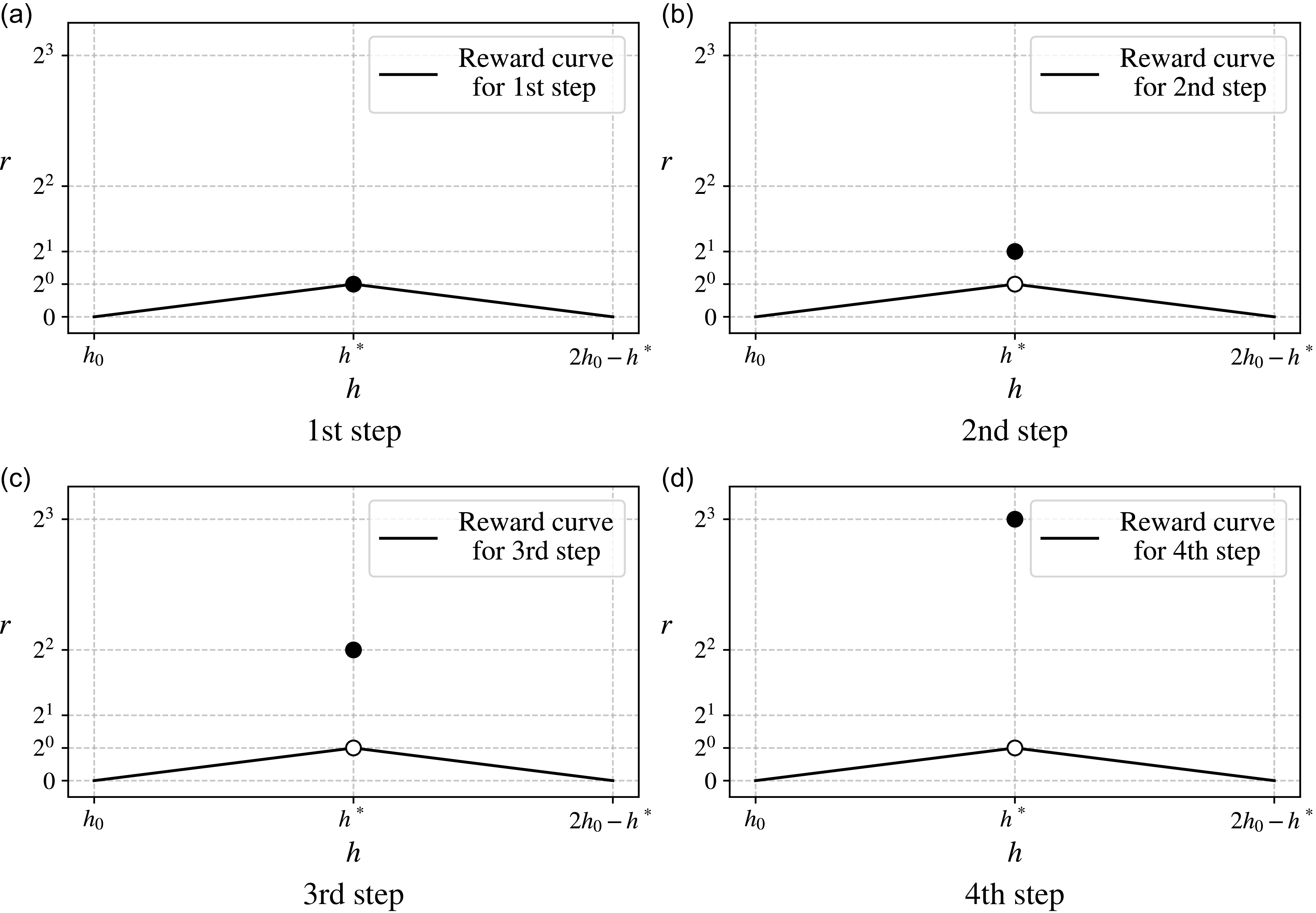
For each trajectory point’s reward function, Fig. 2 shows the reward curves for trajectory points from step 1 to step 4. The 2D visualisation resembles a projection from the z-axis. The x-axis represents the step number, the y-axis shows the altitude and a heat map illustrates the reward distribution. This modification better demonstrates how rewards vary with different altitudes across various steps. When the trajectory point deviates from the target altitude (
 ${h_i}$
 $ \ne {h^{\rm{{\star}}}}$
), the reward is determined by AE function, represented as continuous straight lines. When the trajectory point matches the target altitude (
 ${h_i}$
=
 ${h^{\rm{{\star}}}}$
), the reward abruptly switches to a discontinuous value calculated using an exponential term based on the current step number
 $i$
.
Reward function curves for evaluating trajectory point performance within the first four steps.

By formulating the reward functions of first four steps as a continuous sequence in Fig. 3, it can be observed that when the trajectory point deviates from the target altitude, the reward assessment for each step is similar. However, when the trajectory point does not deviate from the target altitude, the reward value increases exponentially with the increase in the number of steps, and this exponential growth is evident.
The reward exponentially grows with step number when no deviation occurs.

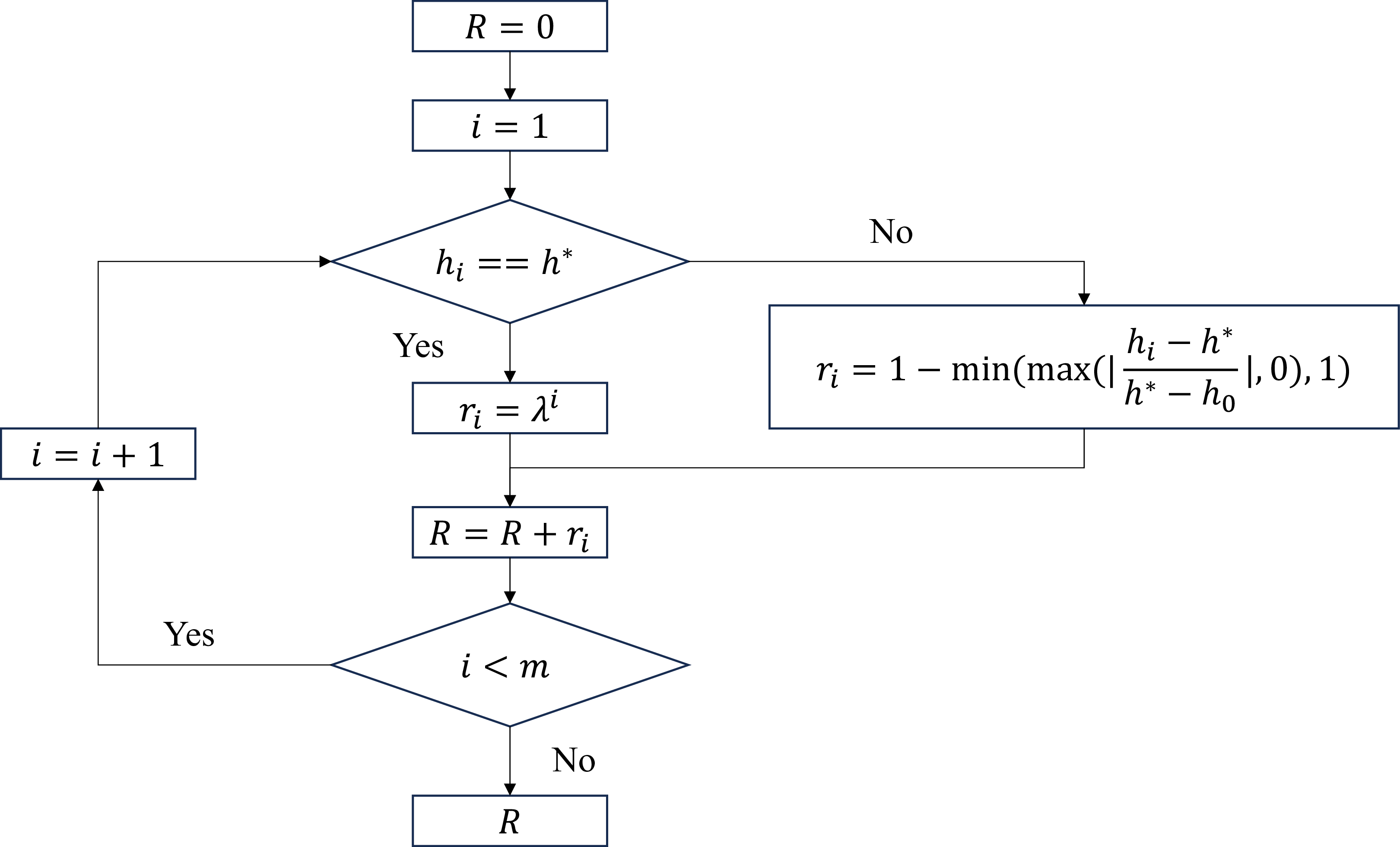
By combining the single-step reward function, if the WIG’s trajectory consists of
 $m$
steps totally, the total trajectory reward
 $R$
can be calculated as
 $R = \sum {_{(i = 1)}^m} \,{r_i}$
, and this process can be demonstrated in a flowchart in Fig. 4.
Flowchart for evaluating the total trajectory reward.

2.2 Mathematical proof
The objective is to design a reward function that prioritises minimising ST first and IAE second, without parameter tuning. Since the AE reward has an upper bound, we can set a lower bound for ST-related rewards to ensure ST takes precedence over IAE. A proof by contradiction is used.
2.2.1 Formulation
If only the
 $m$
-th step (final step) matches the target altitude (
 ${h_i}$
=
 ${h^{\rm{{\star}}}}$
), ST will be
 $m$
. If trajectory points of
 $m$
-th and (
 $m$
−1)-th step remain on target, ST becomes (
 $m$
−1). Extending this logic: if the trajectory matches the target altitude for (
 $m-s$
) consecutive steps before termination, ST decreases as
 $m$
increases. The final step
 $m$
-th must satisfy
 ${h_i}$
=
 ${h^{\rm{{\star}}}}$
to minimise ST, making it the highest priority. Subsequent steps, such as (
 $m$
−1)-th, (
 $m$
−2)-th, are prioritised in reverse order, with previous steps (e.g. 1st step) having the lowest priority. This reasoning ensures that trajectory adjustments prioritise minimising ST by sequentially enforcing alignment from the final step backward.
Since the non-deviation state at
 $m$
-th step is of utmost importance, adjustments to altitude trajectory points from 1st step to (
 $m$
−1)-th step should prioritise maintaining the non-deviation state at step
 $m$
. Specifically, the total reward loss caused by adjustments of 1st step to (
 $m$
−1)-th step must be smaller than the reward gain from adjusting
 $m$
-th step to non-deviation state. This ensures optimisation tools like deep reinforcement learning can search for trajectories with higher rewards, driving the trajectory toward the non-deviation state at
 $m$
-th step. Thus, the inequality must hold as:
 \begin{align} {\sum_{(n = 1)}^{(n = m - 1)}} |\Delta {r_n}| \lt {(\Delta {r_m})^*} \end{align}
where
 ${\rm{\Delta }}{r_n}$
denotes the reward change caused by adjusting the altitude of the trajectory point at
 $n$
-th step. The adjustment can result in total of
 $A_2^2$
= 4 kinds of possible state transition, where the state can either deviate or remain non-deviating.
 ${\rm{\Delta }}{r_m}$
represents the reward gain from adjusting
 $m$
-th step from a deviated to a non-deviated state. The left-hand side of the inequality quantifies the cumulative reward loss from trajectory adjustments at 1st to (
 $m$
−1)-th step, while the right-hand side represents the reward gain from trajectory adjustments at
 $m$
-th step. Given the diverse state transition possibilities at each step and the various distributions of trajectory points in non-deviating states, the values on both sides of the inequality lies within a specific range. To ensure the inequality holds, the maximum value of the left side should be less than the minimum value of the right side. The maximum value of the left side of the inequality (2) can be derived as:
 \begin{align} \max\!\left( \sum_{n=1}^{n = m - 1} \left| \Delta r_n \right| \right)&= \sum_{n=1}^{n = m - 1} \max\!\left( \left| \Delta r_n \right| \right) \nonumber \\[3pt] &= \sum_{n=1}^{n = m - 1} \max\!\left( \lambda^{n-1}- \left(1 - \min\!\left(\max\!\left(\left| \frac{h_i - h^*}{h^* - h_0} \right|\!, 0\right)\!, 1\right)\right)\right) \nonumber \\[3pt]&= \sum_{n=1}^{n = m - 1} \lambda^{n-1}.\end{align}
The minimum value of the right side of the inequality (2) can be deduced as:
 \begin{align}\begin{array}{ll}{{\rm{min}}\!\left( {{{\left( {{\rm{\Delta }}{r_m}} \right)}^{\ast}}} \right)} & = {\rm{min}}\!\left( {{\lambda ^{m - 1}} - \left( {1 - {\rm{min}}\!\left( {{\rm{max}}\!\left( {\left| {\dfrac{{{h_i} - {h^{\ast}}}}{{{h^{\ast}} - {h_0}}}} \right|\!,0} \right)\!,1} \right)} \right)} \right)\\[11pt]& = {\lambda ^{m - 1}} - 1 \end{array} \end{align}
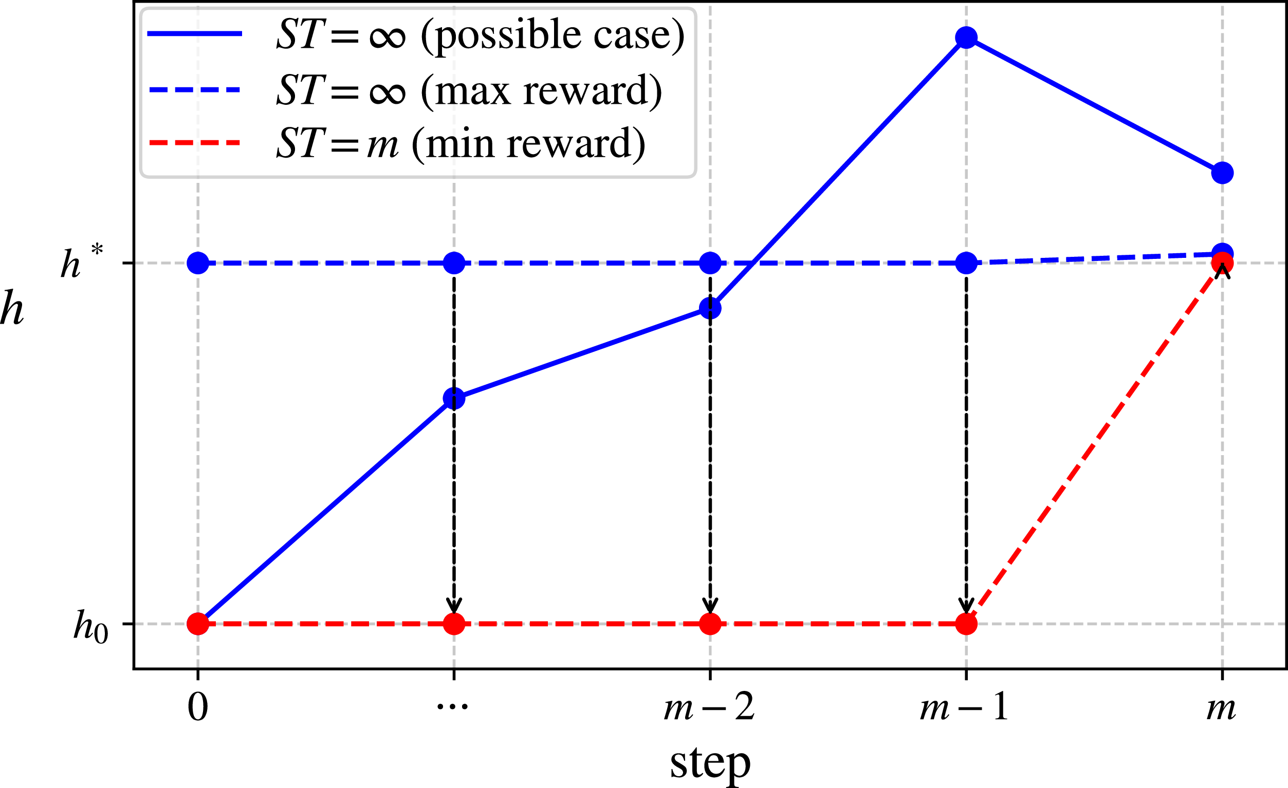
A schematic illustration can help explain the physical meaning. In Fig. 5, the blue dashed line represents the trajectory where ST does not exist (denoted as
 $\infty $
), achieving the maximum reward value. Except for the last trajectory point, which is slightly deviating from the target altitude, the reward value is
 $0.\dot 9$
that asymptotically approaches 1, all other trajectory points remain non-deviating, with reward values calculated as the exponential value
 ${\lambda ^{n - 1}}$
for the
 $n$
-th step.
Trajectory whose ST does not exist with maximum reward and trajectory whose ST =
 $m$
with minimum reward.

The red dashed line represents the trajectory where ST =
 $m$
, achieving the minimum reward value. Except for the last point, which remains non-deviating at the target altitude with a reward value of
 ${\lambda ^{\left( {m - 1} \right)}}$
, all other trajectory points are deviating and remain the initial altitude, with rewards equal to zero.
The black dashed arrows indicate the change at each step for these two extreme cases. The goal is to transform ST from non-existence to ST =
 $m$
, i.e. to reduce ST. The reward changes from 1st to (
 $m$
−1)-th step represent a loss, corresponding to the left side of the inequality (2), while the reward change for the last trajectory point represents a gain, corresponding to the right side of the inequality. To achieve this transition, the gain should logically exceed the loss.
In practice, since the WIG is underactuated, the current state affects the state that can be reached in the next step. Therefore, when adjusting one trajectory point, the other points also tend to change accordingly. In most cases, it is difficult to achieve the two extreme scenarios described above. The solid blue line represents a realistic possible trajectory in Fig. 5.
2.2.2 Feasibility
To guaranteed:
 \begin{align} \mathop \sum \limits_{n = 1}^{n = m - 1} {\lambda ^{n - 1}} \lt {\lambda ^{m - 1}} - 1 \end{align}
The right-hand side is a geometric sequence with common ratio
 $\lambda $
, first term
 ${\lambda ^{m - 2}}$
, and number of terms
 $\left( {m - 1} \right)$
. Its sum is:
 \begin{align}S = \frac{{{\lambda ^{m - 1}} - 1}}{{\lambda - 1}},{\rm{\;\;\;\;}}\lambda \ne 1 \end{align}
So the inequality becomes:
 \begin{align}{\lambda ^{m - 1}} - 1 \gt \frac{{{\lambda ^{m - 1}} - 1}}{{\lambda - 1}} \end{align}
Therefore, when
 $\lambda \gt 2$
, the inequality (2) holds. In practical scenarios, such as the underactuated nature of the WIG discussed in the engineering context, reaching the considered boundaries is often challenging. Therefore, the actual benefit is likely underestimated, while the loss is overestimated. As a result, the condition generally holds even when the exponential base value equals 2. Thus,
 $\lambda \geqslant 2$
, the inequality (2) is valid.
2.2.3 Extension
After ensuring that the final step, the
 $m$
-th step, does not deviate from the target altitude, the remaining problem is how to prevent the (
 $m$
−1)-th trajectory point from deviation. Building on the preceding analysis, it can be proven likewise that:
 \begin{align} \mathop \sum \limits_{n = 1}^{n = m - 2} \!\left| {{\rm{\Delta }}{r_n}} \right| \lt \left( {{\rm{\Delta }}{r_{m - 1}}} \right) \end{align}
which ensures that the reward gain for the (
 $m$
−1)-th trajectory point not deviating from the target altitude exceeds the loss from any adjustments in the previous
 $m$
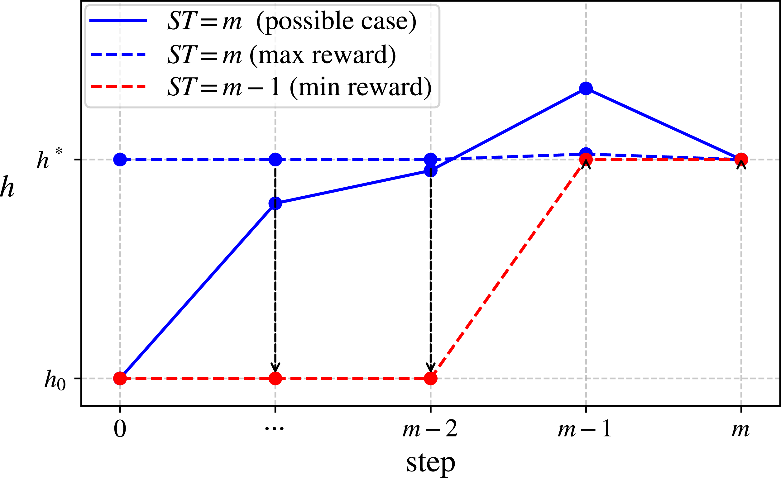
−2 steps. The physical meaning is illustrated in Fig. 6, depicting extreme cases where the trajectory is ST =
 $m$
with maximised reward, and ST =
 $m$
−1 with minimised reward. While both trajectories exhibit no deviation at the final trajectory point, the former only deviates slightly at the (
 $m$
−1)-th trajectory point, whereas the latter deviates at all trajectory points except the (
 $m$
−1)-th trajectory point. The inequality (8) guarantees that the performance of the first
 $m$
−2 trajectory points can be sacrificed to facilitate the transition of the (
 $m$
−1)-th trajectory point toward not deviating from the target altitude. By extension, this kind of inequality allows sequential adjustment of trajectory points from the end backward, gradually aligning them with the target altitude.
Trajectory whose ST =
 $m$
with maximum reward and trajectory whose ST =
 $m$
–1 with minimum reward.

3.0 Validation
3.1 Reward functions
In practical engineering applications, an acceptable deviation interval
 $\varepsilon $
is defined around the target value. When the WIG’s altitude falls within this interval, it is considered to have reached the target altitude. Based on this, the reward function proposed in this study can be modified as:
 \begin{align}{r_{sc}}\!\left( i \right) = \left\{ \begin{array}{l@{\quad}l}{r_c}\!\left( i \right), & {}{\left| {{h_i} - {h^{\ast}}} \right| \gt \varepsilon }\\[4pt]{\lambda ^{i - 1}}, {}&\left| {{h_i} - {h^{\ast}}} \right| \le \varepsilon \end{array} \right. \end{align}
where
 ${r_c}\!\left( i \right)$
is the AE function defined as:
 \begin{align}{r_c}\!\left( i \right) = 1 - {\rm{min}}\!\left( {{\rm{max}}\!\left( {\left| {{\rm{\;}}\frac{{\left| {{h_i} - {h^{\ast}}} \right| - \varepsilon }}{{\left| {{h^{\ast}} - {h_0}} \right|}}}\! \right.,0} \right)\!,1} \right) \end{align}
The total reward for the complete trajectory is:
 \begin{align} {R_{sc}} = \mathop \sum \limits_{i = 1}^m {r_{sc}}\!\left( i \right) \end{align}
For comparison, the conventional multi-objective function evaluates the AE reward at each step and assesses the entire trajectory for ST. The total reward for the complete trajectory is expressed as:
 \begin{align} {R_{mo}} = \mathop \sum \limits_{i = 1}^m {r_c}\!\left( i \right) + k \, {\ast} \, {r_s} \end{align}
where the first term, sum of
 ${r_c}$
for all deviated trajectory points represents the IAE, and the second term represents the ST. The two terms are related by the weight
 $k$
, which can be adjusted to balance their relative importance in the reward function.
 ${r_s}$
measures the ST of the trajectory:
 \begin{align}{r_s} = {\rm{min}}\!\left\{ {\left. {n \in \mathbb{N}} \right|\mathop {{\rm{sup}}}\limits_{i \geqslant n,i \le m} \left| {{h_i} - {h^{\ast}}} \right| \le \varepsilon } \right\} \end{align}
where sup is the abbreviation for ‘supremum’, representing the least upper bound.
 $\mathbb{N}$
denote the set of positive integers.
3.2 Method
Deep reinforcement learning is employed to optimise the trajectory by evaluating its reward value, seeking the one with the maximum reward, thereby obtaining the optimal trajectory and verifying whether the reward function meets the design expectation. It learns an optimal policy through continuous interaction, maximising the cumulative reward to address high-dimensional problems that are difficult to handle with conventional methods. Accordingly, in this study, the WIG continuously attempts to adjust its trajectory to seek one that achieves the maximum reward (Fig. 7). The specific algorithm used is proximal policy optimisation (PPO) [Reference Schulman, Wolski, Dhariwal, Radford and Klimov25], a policy gradient method that balances exploration and exploitation in reinforcement learning, which is implemented with the open-source code [Reference Liu, Li, Wang and Zheng26].
Deep reinforcement learning for the WIG to search the optimal trajectory.

The computation was performed on hardware comprising an AMD Ryzen 5 5600G 3.9 GHz processor with 16 GB DDR4 2666 MHz RAM. Each iteration required approximately 4 GB of RAM and took about 20 seconds to complete.
Regarding training stability, a three-phase hyperparameter scheduling strategy was implemented: Phase 1 (learning rate: 5e-5, entropy coefficient: 0.01) continued until no reward improvement was observed for 1,000 consecutive iterations; Phase 2 (learning rate: 1e-5, entropy coefficient: 0.005) proceeded until 1500 iterations without improvement; Phase 3 (learning rate: 1e-6, entropy coefficient: 0.0025) continued until 2,000 iterations showed no further enhancement. The progressively reduced learning rate ensured convergence stability, while the decreasing entropy coefficient effectively balanced exploration and exploitation.
To ensure robustness, eight independent trials with different random seeds are conducted for each case. In addition to the presentation of the highest-reward trajectory as the primary result, a statistical analysis of altitude data is performed at each waypoint. The 25th–75th percentile range is calculated to demonstrate the distribution encompassing 50% of the optimised results.
3.3 Settling time
3.3.1 WIG model
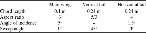
The case is about a small WIG’s altitude change in the longitudinal plane, its model and coordinate frames for motion description, grid for aerodynamic calculation and kinetic analysis are shown in Fig. 8. Table 1 summarises the geometric configuration of the wing components for the WIG. It has three degrees of freedom: horizontal and vertical translations, and pitch. The two control inputs are the elevator deflection and throttle. The state variables include displacement, pitch angle, linear velocity, angular velocity, linear acceleration and angular acceleration. Among these, the flight altitude is extracted. The dynamic and kinematic models for calculating the WIG’s motion response are referenced from the study [Reference Hu, Zhang, Ding, Jiao, Zhang and Zhang4, Reference Hu, Li, Zhang and Zhang5].
Geometric parameters of wing parts in the WIG

The virtual small WIG and its coordinate frames.

The WIG’s aerodynamics is simulated by vortex lattice method, and the ground effect is simulated by image method. A vortex element and a corresponding control point are assigned to each panel. The total force
 ${\bf{F}}$
and moment
 ${\bf{M}}$
with respect to the origin are obtained by summing the individual contributions from all vortex elements, as:
 \begin{align} {}&{{{\bf{F}}_i} = \rho {{\rm{\Gamma }}_i}\!\left( {{{\bf{V}}_\infty } + {{\bf{v}}_i}} \right) \times {{\bf{l}}_i}} \nonumber \\[3pt]&{{\bf{F}} \, \,= \mathop \sum \limits_{i = 1}^N {{\bf{F}}_i}} \nonumber \\[3pt] {}&{{\bf{M}} = \mathop \sum \limits_{i = 1}^N {{\bf{F}}_i} \times {{\bf{r}}_i}} \end{align}
where
 $\rho $
is the air density.
 ${{\rm{\Gamma }}_i}$
denotes the strength of the vortex,
 ${{\bf{l}}_i}$
represents the vector of the vortex segment oriented transversely,
 ${{\bf{V}}_\infty }$
is the freestream velocity vector, and
 ${{\bf{v}}_i}$
indicates the local velocity disturbance at the midpoint of the vortex segment.
Regarding the aerodynamics of the WIG, when an elevator deflection
 $\delta $
is executed during flight, the forces acting on the vehicle, as depicted in Fig. 8, can be decomposed into two distinct components. The first component consists of the aerodynamic forces and moment applied to the entire craft: lift
 ${F_L}$
, drag
 ${F_D}$
and pitching moment
 $M$
. These represent the resultant forces and moment at the centre of gravity, derived from the combined contributions of the horizontal stabiliser (lift
 ${F_{L,h.s}}$
, drag
 ${F_{D,h.s}}$
, pitching moment
 ${M_{h.s}}$
), the vertical tail (lift
 ${F_{L,v.t}}$
, drag
 ${F_{D,v.t}}$
, pitching moment
 ${M_{v.t}}$
) and the main wing (lift
 ${F_{L,m.w}}$
, drag
 ${F_{D,m.w}}$
, pitching moment
 ${M_{m.w}}$
). The second component is the thrust
 $T$
generated by the propulsion system. Therefore, the total resultant forces and moment acting on the WIG craft within this planar force system are expressed as:
 \begin{align}\begin{array}{l} {}{{F_x} = {F_D} + T \cdot {\rm{cos}}\!\left( \alpha \right)}\\[6pt] {}{{F_z} = {F_L} + T \cdot {\rm{sin}}\!\left( \alpha \right)}\\[6pt] {}{{M_y} = M + T \cdot {L_2}}\end{array} \end{align}
where
 $\alpha $
denotes the pitch angle during actual flight operations, and
 ${L_2}$
represents the vertical distance between the centre of gravity
 $CG$
and the line of action of the thrust force when the pitch angle is
 ${0^ \circ }$
. Then, the WIG’s aerodynamics will be fed into the its motion simulation as:
 \begin{align}\begin{array}{l} {}{{\dot{\bf u}} = {\bf{u}} \times \omega + {\bf{C}}_{\bf{g}}^{\bf{b}} \cdot \left( {\frac{{\bf{F}}}{m} + {{\bf{g}}^{\bf{n}}}} \right)}\\[10pt] {}{\dot \omega = {{\bf{I}}^{ - 1}}\left( { - \omega \times {\bf{I}}\omega + {\bf{M}}} \right)}\end{array} \end{align}
where
 ${\bf{F}}$
is [
 ${F_x}$
,0,
 ${F_z}$
] and
 ${\bf{M}}$
is [0,
 ${M_y}$
,0].
 ${\bf{u}}$
,
 $\omega $
are line and angle velocity, and
 ${\dot{\bf u}}$
and
 $\dot \omega $
are the corresponding accelerations.
 $m$
represents mass of the WIG, and
 ${{\bf{g}}^{\bf{n}}}$
signifies the acceleration of gravity.
 ${\bf{C}}_{\bf{g}}^{\bf{b}}$
is the coordinate frames’ transformation matrix.
 ${\bf{I}}$
denotes moment of inertia.
For the current validation scenario, the initial altitude of the WIG is
 ${h_0}{\rm{\;}}$
= 0.3
 $c$
, and the target altitude is
 ${h^{\rm{{\star}}}}$
= 0.6
 $c$
, where
 $c$
is the chord length of the wing,
 $c$
= 0.4 m. The entire trajectory consists of 24 steps, with each time step lasting 0.02 s. When measuring settling time, the acceptable deviation is
 $\varepsilon {\rm{\;}}$
=
 ${10^{ - 3}}\left| {{h^{\rm{{\star}}}} - {h_0}} \right|$
. The acceptable deviation parameter
 $\varepsilon $
is selected in this study to reduce computational costs associated with high-dimensional problems while maintaining adequate validation of the algorithm’s performance. For practical WIGs’ applications, the allowable deviation should be determined based on specific performance requirements, while also considering sensor errors (including altitude measurement inaccuracies) and sampling rate limitations.
The elevator’s deflection
 $\delta $
is constrained by both the deflection angle limits of
 $ \pm {10^ \circ }$
and the angle-of-attack limits of
 $ \pm {10^ \circ }$
. Assuming the current pitch angle is
 ${\alpha _c}$
, with horizontal and vertical velocities denoted as
 ${V_x}$
and
 ${V_y}$
respectively, the corresponding quasi-static angle-of-attack is
 ${\alpha _q}$
=
 ${\rm{arctan}}\!\left( {{V_y}/{V_x}} \right)$
. Thus, the feasible range for the elevator deflection falls within the interval [max(
 $ - {10^ \circ } - {\alpha _c} - {\alpha _q}$
,
 $ - {10^ \circ }$
), min(
 ${10^ \circ } - {\alpha _c} - {\alpha _q}$
,
 ${10^ \circ }$
)] to prevent flow separation and stall. The other control input is engine thrust, and its maximum is
 $T$
= 7.06 N.
In practical engineering applications, factors such as sensor noise (which affects state acquisition accuracy), actuator delays (impacting timely control output), model uncertainties (causing deviations between expected and actual actions), and safety constraints (further limiting the manoeuvrability of the underactuated WIGs) do indeed introduce significant challenges. While these external constraints are not explicit requirements of the core algorithm proposed in this study, the algorithm’s performance is undoubtedly influenced by these practical factors. Typically, when the effects of such practical factors are modeled as Gaussian distributions, the proposed method would yield a single trajectory that maximises the expected reward in a statistical sense under such distributions. Provided these practical factors are appropriately modeled without ambiguity, the proposed method guarantees a unique solution.
3.3.2 Result
Conventional multi-objective function approaches typically involve testing multiple weight values through trial and error, to ensure the trajectory appear the smallest ST and the smallest IAE during the state transition. In this study, the weight
 $k$
is respectively set to multiple values between 0 and
 ${10^2}$
for constructing different reward functions.
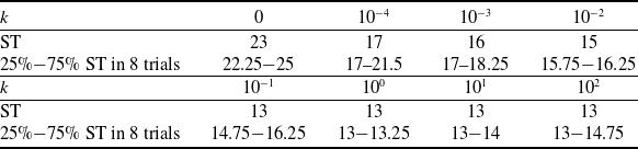
To demonstrate the statistical significance of the deep reinforcement learning results, the 25th–75th percentile range is now displayed for each trajectory point based on eight training runs, indicating that 50% of the learning outcomes fall within this range. The resulting trajectories obtained via deep reinforcement learning are shown in Figs 9 and 10. Table 2 summarises their ST performance, including the 25th−75th percentile range of ST data from eight optimisation trials. Figure 9 presents a composite view of all trajectories, while Fig. 10 displays a magnified view of the trajectories corresponding to increasing weight value
 $k$
in ascending order, to highlight specific details. It can be found that as the weight of ST term increases, ST decreases gradually until stabilising at 13 steps.
Settling time (ST) of trajectories by multi-objective reward functions with varying
 $k$

Overall trajectories by multi-objective reward functions
 ${R_{mo}}$
with varying
 $k$
.

Magnified views of trajectories by multi-objective reward functions
 ${R_{mo}}$
with varying
 $k$
.

In the proposed reward function,
 $\lambda $
is required to be at least 2.
 $\lambda $
is sequentially set as 2, 3, 4 in
 ${r_{sc}}$
to construct the reward functions and put into the deep reinforcement learning for the corresponding trajectories, as shown in Fig. 11. The first two subfigures illustrate all trajectories overlaid in a single plot, whereas the following subfigures provide zoomed-in views of trajectory segments corresponding to progressively increasing base value
 $\lambda $
. Table 3 compares the settling time of trajectories achieved by the proposed reward function across different parameter configurations. It can be found that when
 $\lambda \geqslant 2$
, the corresponding trajectories stabilise at the 13-th step.
Overall and magnified views of trajectories by the proposed reward function
 ${R_{sc}}$
with varying
 $\lambda $
.

Unlike the conventional multi-objective function approach which requires multiple adjustments to the weight
 $k$
, the proposed reward function can directly reach the extreme without trial-and-error iterations. The three trajectories of
 $\lambda = 2$
,
 $\lambda = 3$
and
 $\lambda = 4$
should theoretically be identical, because under the same condition that ST has been minimised, the trajectory points before ST are guided solely by AE function. However, the resulting trajectory points do not perfectly coincide. The reason is that the WIG’s state space is very complex. Due to limited computational resources, deep reinforcement learning performs a limited search, making it challenging to achieve the globally maximum reward. Nevertheless, the trend of overall ST minimisation remains consistent. Therefore, a simpler example with a smaller state space is used in subsequent verifications to minimise IAE.
Settling time (ST) of trajectories by the proposed reward functions with varying
 $\lambda $

3.3.3 Notes
For the conventional approach, achieving the target trajectory requires a trial-and-error process of adjusting the weighting coefficient across values such as
 $k = 0$
,
 $k = {10^{ - 4}}$
,
 $k = {10^{ - 3}}$
,
 $k = {10^{ - 2}}$
,
 $k = {10^{ - 1}}$
,
 $k = {10^0}$
and
 $k = {10^1}$
and
 $k = {10^2}$
. As
 $k$
increases, the trajectory gradually evolves and stabilises at the target. This process exemplifies the time-consuming tuning that conventional methods require. In stark contrast, the proposed method directly generates this target trajectory without the need for any iterative parameter adjustments, thus eliminating this costly trial-and-error phase.
Optimisation iteration counts for trajectory generation by multi-objective
 ${R_{mo}}$
and the proposed
 ${R_{sc}}$
reward function

Figure 12 comparatively plot altitude-distance trajectories by multi-objective
 ${R_{mo}}$
and the proposed
 ${R_{sc}}$
reward function in the spatial domain. The core objective of the proposed method is not primarily to achieve the fastest possible obstacle avoidance, but rather to prioritise rapid stabilisation at the target altitude (minimising settling time) first, followed by minimisation of the overall deviation. An overly aggressive climb would typically cause significant overshoot, resulting in increased settling time and larger deviation, which contradicts our design goals. The proposed method is applicable to both climbing and descending manoeuvres, achieving fast stabilisation with minimal deviation in scenarios which involves climbing pre-obstacle, descending post-obstacle or adjusting altitude based on mission efficiently. To prevent obstacle collisions, sufficient safety distance must be maintained before initiating avoidance manoeuvres. Similarly, adequate safety altitude must be preserved during descent to prevent water impact.
Altitude-distance trajectories by multi-objective
 ${R_{mo}}$
and the proposed
 ${R_{sc}}$
reward function in the spatial domain.

Table 4 presents the parameter tuning cost of the conventional methods along with lower cost of the proposed method. The conventional multi-objective reward function requires eight parameter-tuning attempts and approximately 67,552 iterations to identify the target trajectory. In contrast, the proposed reward function achieves the same objective in only 7,522 iterations without requiring any parameter tuning. This provides substantial advantage in computational efficiency when comparing single optimisation against multiple tuning attempts.
The variations in elevator deflection and engine thrust for trajectories obtained by both the conventional method and the proposed method are illustrated in Fig. 13. While the differences are minor during the initial phase, significant discrepancies emerge during the stabilisation phase.
Control input by multi-objective
 ${R_{mo}}$
and the proposed
 ${R_{sc}}$
reward function in the time domain.

3.4 Integrated absolute error
3.4.1 Model
A simple second-order response model for single-degree-of-freedom altitude adjustment is used for validation. The model’s motion response is defined as:
 \begin{align}\begin{array}{l} {}{a = \frac{{F - mg}}{m}}\\[5pt] {}{v = v + a{\rm{\Delta }}t}\\[5pt]{h = h + v{\rm{\Delta }}t}\end{array} \end{align}
where
 $m$
= 1 kg,
 $F \in \left[ {0,20} \right]$
N,
 $g\;$
= 10
 ${\rm{m}}/{{\rm{s}}^2}$
and
 ${\rm{\Delta }}t\;$
= 0.1 s.
 $a$
is the acceleration, and
 $v$
is the velocity. The initial altitude is
 ${h_0}$
= 0 m and
 ${v_0}{\rm{\;}}$
= 0 m/s. The target altitude is
 ${h^{\rm{{\star}}}}$
= 0.5 m, and the acceptable deviation ratio is
 $\varepsilon \;$
=
 ${10^{ - 2}}\left| {{h^{\rm{{\star}}}} - {h_0}} \right|$
.
3.4.2 Result
The control group is set up using a single-objective function
 ${r_s}$
that only considers the minimisation of ST. Since
 ${r_s}$
ensures the fastest attainment of the target altitude without constraining the performance of the transition, it results in multiple trajectories with varying IAE values. Through deep reinforcement learning, total of 200 trajectories are obtained for
 ${r_s}$
to reach the extremum, while
 ${r_{sc}}$
yields a single trajectory. Their comparison is shown in Fig. 14. It can be observed that 200 trajectories produced by
 ${r_s}$
are dispersed. The proposed reward, under the condition of achieving the minimum ST, directly obtains the trajectory with the minimum IAE.
Trajectories obtained by the single-objective function
 ${r_s}$
and the proposed
 ${r_{sc}}$
.

4.0 Conclusion
For a WIG in descending and ascending scenarios to achieve rapid stabilisation at the target altitude while minimising trajectory deviation during the adjustment process, this study proposes a reward function that establishes ST minimisation as the superior objective to IAE minimisation, eliminating the need for iterative adjustment of weight required by conventional multi-objective methods. The proposed reward introduces the basic absolute error function and modifies it into the discontinuous form for each step. When trajectory points deviate from the target altitude, reward will be calculated based on AE values. Once the target altitude is reached, the reward will be given exponentially with the current step number. Through appropriate exponential base setting, the function ensures that positive rewards for reducing ST outweigh the reward losses from adjusting previous trajectory points. It guides the trajectory to prioritise reducing ST while suppressing deviations during the transition. Mathematical proof confirms the feasibility of this reward function, which is validated through a WIG’s altitude adjustment via deep reinforcement learning.
Compared to conventional multi-objective methods and single-objective functions optimised for ST, the proposed reward function achieves an optimal solution with the smallest settling time, also achieving the lowest trajectory deviation. The reward function requires no parameter tuning and provides an efficient solution for WIG’s trajectory planning, first ensuring the fastest stabilisation and then achieving minimal deviation.
Acknowledgements
The authors gratefully acknowledge the constructive comments from the anonymous reviewers and the editor, whose insights and suggestions significantly improved the quality of this manuscript.
Data availability statement
Source codes are available at https://github.com/HuanHu2019/Priority-based_reward_function_for_fast-settling_and_low-deviation_trajectory_planning
Competing interests
The authors declare that they have no known competing financial interests or personal relationships that could have appeared to influence the work reported in this paper.