

Introduction
A 3D map of objects of an environment is useful in many issues of precision agriculture. For instance, it could be used to localise a robot on the field, to prevent it from bumping into obstacles or to plan a trajectory the robot would take to reach its destination (Roh et al., Reference Roh, Sung and Chung2013). Next, a 3D model could be used to get information about the plant development (Garrido et al., Reference Garrido, Paraforos, Reiser, Vazquez Arellano, Griepentrog and Valero2015), to evaluate the shape / density of a tree silhouette for precision spraying application (Wellington, Reference Wellington, Campoy, Khot and Ehsani2012). And finally, a 3D model could even be used to pick fruits (Dzitac et al., Reference Dzitac and Mazid2012), to measure the size of the trees (Ehlert et al., 2009) or to distinguish weed from maize plants (Andujar et al., Reference Andujar, Rueda-Ayala, Moreno, Rosell, Escola, Valero, Gerhards and Griepentrog2013).
To make an autonomous field robot it has to include all necessary sensors and logic in order to localise itself, to build a map of the environment and to possibly plan a path it would take to move to a new position. The environment sensing can be accomplished by using simple ultrasonic or infra-red sensors that produce trivial readings, but if we want to get more accurate results, complex sensors should be used, such as cameras, depth cameras, or single/multi-channel LIDAR scanners that produce more detailed results.
Some limitations can be overlooked if we know that the robot will only have to avoid obstacles that are on the ground, where a simple 2D LIDAR can be used to drive between them. In more complex environments, where parts of the objects hang and obstruct the robot, there are more problems. In this cases it is necessary to build a 3D model of the scene. An example of such approach was described by Ben-Tzvi et al. (2010), where two cameras were used to calculate a depth information by analysing corresponding pixel pairs. The work from Jung et al. (Reference Jung and Lyou2014) is based on the use of digital camera and a projector that emits structured light on to the target and depth information is recorded by measuring the intensity of the reflected light. The closer the object is, the bright the colour and vice versa. The most expensive sensors are the 3D LIDAR scanners (Roh et al., Reference Roh, Sung and Chung2013). They use laser light to measure the distance from the scanner to a point of the scene. In comparison to the ordinary 2D models, the 3D versions have multiple channels. This means they take measurements on different planes, but are limited with the number of channels, for instance 16, 32 or 64.
If a 3D LIDAR scanner is used on a field robot it would make possible for such a robot to sense the environment and navigate between the obstacles (Roh et al., Reference Roh, Sung and Chung2013). It would be able to detect the crop lines when placed in a field and navigate between them without destroying the plants. Next, it could detect fruits or crops with an intent to harvest them by focusing on the shapes measured by a 3D depth sensor (Dzitac et al., Reference Dzitac and Mazid2012), or it could record the shape of the tree crown canopy (Wellington, Reference Wellington, Campoy, Khot and Ehsani2012) to adjust the dosage rate of pesticides based on the thickness of the tree crown. If there are no branches, the valves are shut, with branches the valves are open and if there as just a few branches, the valves are partly open.
It is useful to know the size of fruit or plants. If a fruit producer wants to make a prognosis about the yield of the harvest (Stajnko et al., Reference Stajnko, Lakota and Hocevar2004), he has to know the number and size of fruit. If a forester wants to estimate the biomass (Ehlert et al., 2009) of a tree it has to know its high and diameter or a volume. In all these cases having a 3D model of the scene would be useful and the system like this could be a part of an autonomous farming robot.
One of the most important parts of the software for such a robot would represent a SLAM (simultaneous localisation and mapping) algorithm. The most well-known SLAM algorithms are Gmapping (Grisetti et al., 2005 and 2007) and Hector mapping (Kholbrecker et al., Reference Kohlbrecher, Meyer, Graber, Petersen, Klingauf and Stryk2013). To localize and create a map of the environment Gmapping relays on the use of Rao-Blackwellized particle filter that minimizes the number of particles to reduce local uncertainty. The approach is optimised for long-range data captured by a LIDAR scanner and therefor suitable for large areas. But in order to work it needs additional data from the robots’ odometry.
As tested in a previous work by Lepej et al. (Reference Lepej and Rakun2016), Hector mapping is not proven to be the best choice for outdoor environments due to changing conditions and unstructured pattern of the surrounding objects. Instead, an image analysis-based approach is suggested because it utilises image registration techniques done in the frequency domain. In comparison to Gmapping the presented approach works without any odometry data.
The goal of this work is to investigate the possibility of using two non-costly 2D LIDAR scanners to reconstruct a 3D scene, instead of using a more expensive multi-channel sensor, by applying an alternative SLAM approach. To test the approach a small field robot was fitted with two 2D sensors and the tests were conducted in indoor as well as outdoor environment.
Materials and methods
To capture the data needed to build a 3D representation of the world, a small autonomous field robot was used in this experiment. The robot is originally mounted with one LIDAR scanner (SICK TIM310) that enables it to move between the crop lines, but to build a 3D model an additional sensor (SICK LMS111) was mounted to record shapes on vertical plane.
Then to build a 3D model of the scene a two-step approach was used. The first step represents the mapping algorithm (SLAM) that builds a 2D map of the environment. It is then followed by the second step, point cloud assembly, which adds additional dimension to the first.
Instrumentation - Cornstar robot
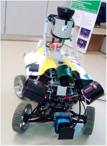
To test the approach a small robot was used, build as part of a student reserch project. The robot has four components: sensors, embedded electronics, mehanics and actuators. qThe mahanical part of the robot is build as a four-wheel drive, where the two axles can turn indivitualy, a three phase motor that enables the robot to move and automatic gearbox with one backward and two forward speed transition. To spray the robot also has two electo-magnetic valves, two nozzles and a preassured reservoir. The sensory part of the robot includes the LIDAR scanners and one on-board digital camera. All meassurements on the robot are captured by an embedded computer with ROS and LINUX installed on it. It job is to process the data and make new decisions in order to autonomously drive the whole platform. The robot is depicted on Figure 1.
Cornstar robot with two mounted LIDAR scanners. The LMS111 is mounted horizontally and TIM310 vertically.

Methods – SLAM
In order to build a 2D map of the environment and localise the robot on a plane the SLAM algorithm takes measurements from the horizontally mounted LIDAR scanner (Grasetti et al., 2007; Kohlbrecker et al., Reference Kohlbrecher, Meyer, Graber, Petersen, Klingauf and Stryk2013; Lepej et al., Reference Lepej and Rakun2016). Based on the relative position of the robot a static transformation into 3D space for the data measured by the second, vertical LIDAR scanner is made. By doing so and combining multiple readings in to the same space a 3D model of the environment is build. To achieve this 3D model assembler in ROS and point cloud library were used to construct a 3D model of the world.
Methods – SLAM - Phase Correlation
To calculate displacement between each consecutive measurement, phase correlation was chosen as described in (Gonzalez & Woods, Reference Gonzalez and Woods2001) and (Stone, Reference Stone2001). The correlation works by comparing two images, where the first is a reference and the subsequent one is a template. Since the measurements are semi-identical, looking from a signal point of view, they have almost the same energy distribution. This means the correlation reaches a maximum value when both images are registered. In addition, if the correlation is computed in frequency domain, the translation and rotation are separated and presented in the phase (translation) and amplitude (rotation) spectrum, without having an effect on to another, as in spatial space. So the problem of finding the right parameters can be solved separately.
The translation of the semi-identical signals in spatial space only affects the phase spectrum of the frequency transform. As the signals are semi-identical their phase compensates but preserves their linear part. This produces a maximum global value with coordinates (c x , c y ) that corresponds to the translation on the X and Y axes. If the log-polar transform is used before phase correlation, phase correlation could also be used to calculate rotation. To calculate the correlation, the following equation is applied:
 $$I_{1} \left( {x,y} \right)^{\circ}I_{2} \left( {x,y} \right){\equals}{1 \over {MN}}\mathop \sum\limits_{m\,{\equals}\,0}^{M{\minus}1} \mathop \sum\limits_{n\,{\equals}\,0}^{N{\minus}1} I_{1}^{{\asterisk}} (m,n)I_{2} (x{\plus}m,y{\plus}n)$$
where I 1 (x,y) and I 2 (x,y) represent a 2D signal (image) with M x N pixels in size and I 1 * a complex conjugate of I 1 . By applying the convolution theorem, Eq. 1 can be written as:
 $$I_{1} \left( {x,y} \right)^{\circ}I_{2} \,\left( {x,y} \right)\Leftrightarrow S_{1}^{{\asterisk}} \,\left( {u,v} \right)\,S_{2} \left( {u,v} \right)$$
where S 1 * and S 2 correspond to frequency transforms of the input signals I 1 and I 2 . Based on the convolution theorem the correlation in frequency domain can simply be calculated by multiplying the complex conjugate of the frequency transform of the first by the frequency transform of the second signal.
By transforming measurements and depicting them in spatial space, the consecutive reading shows up as translated outlines of the objects in the scene. Once these displacements are calculated with the help of Eq. 2, they are used to calculate real displacements on both sides. Both displacements are then simply used to compute new vectors with an origin starting at (0,0) located at the beginning of the row, approximately half the distance from each side of the row. Both vectors are then used in simple vector summation which reveals the true movement vector that is the difference along the X and Y axes, along with the new coordinates of the origin for new iteration.
Methods – SLAM – Data Filtering
In real environments the distance between the crop rows may vary, and if the robot is located too close to one side, it can pick up distance readings from the neighbouring row. This can be eliminated in some cases by setting the maximum valid distance reading in ROS’s SICK laser finder node. However, in order to eliminate it completely, a pre-processing filtering step is recommended. A statistical approach was chosen to eliminate this kind of reading. By calculating a median distance for each crop row an interval of valid readings was computed. It comprised of 66.66% of all readings that were closest to the median. Since the majority of the distances in all readings belong to the first row, the marginal distances were filtered out.
Methods – SLAM – Estimating pose and orientation
Different crop plant rows can have versatile structures that produce very different environmental conditions. Our approach to this problem is based on image registration, where we chose phase correlation. It computes the information about the template position on a corresponding original image. Our goal was to estimate an angular shift in successive measurements that corresponds to the differences in translation and rotation on images. We have split these two problems, where we need to calculate phase correlation separately for the estimation of position and orientation. Therefore, we need two different data scan transformations between two distinct successive readings. First, we will describe laser data transformation, which is essential for the phase correlation that is used to estimate the pose.
Methods – SLAM – LIDAR scanner data transformation
This transformation adds an additional dimension to the horizontal laser scan data. The first transformation from LIDAR scanner scans to a 2D signal (image) is done, which is actually a projection of laser scan data into a two-dimensional scaled grid map.
Eq. 3 describes the grid map transformation for linear movement estimation. Transformation is performed for every measured distance set captured by the LIDAR scanner, where only valid data is considered that is greater than 0 and smaller than the maximum range of the LIDAR scanner. For each piece of LIDAR scanner data, the x l and y l coordinates of the 2D signal are calculated. The same conditions are considered for rotational estimation, where for the rotational estimation the data scan transformation is performed and the whole transformation is described by Eq. 5. Laser data transformation uses threshold limits, which are defined by user settings. Users can define the maximum and the minimum laser range, which should be LIDAR scanner specific and depending on the environment.
 $$\left[ {\matrix{ {x_{l} } \cr {y_{l} } \cr } } \right]{\equals}\left[ {\matrix{ {{{round\left( {({\rm cos}\left( {\beta )} \right)\,{\asterisk}\,lrf(i)} \right)} \over {res}}{\plus}I_{w} } \cr {{{round\left( {({\rm sin}\left( {\beta )} \right)\,{\asterisk}\,lrf(i)} \right)} \over {res}}{\plus}I_{h} } \cr } } \right]$$
 $$\beta \,{\equals}\,deg2rad(i{\plus}45)$$
Pose estimation is a linear translation, calculated with the help of a parameter that represents a current laser beam angle. We need to add 45° to obtain the correct orientation of the LIDAR scanner. In our case, we can get a 270 LIDAR scanner measurement, but 180 is used, owing to occluded areas where the wheels of the robot obscure the view. Each measurement, defined by angle i, has a corresponding distance measurement noted with irf (i). The parameter res is the resolution of the signal I with a size of (I w ,I h ). For angular estimation, x a and y a signal positions are calculated, where the parameter range max is used to scale the given LIDAR scanner range into a signal, which has a size two times greater than the LIDAR scanner angular resolution to gain sub-pixel accuracy. The y component is presented as angle data.
 $$\left[ {\matrix{ {x_{a} } \cr {y_{a} } \cr } } \right]{\equals}\left[ {\matrix{ {{{round(lrf(i)\,{\asterisk}\,I_{h} )} \over {range_{{max}} }}} \cr i \cr } } \right] $$
By applying Eq. 3 and Eq. 5 to the original data sets produced by the LIDAR scanner, two 2D point clouds are constructed, and two more for the next measured data sets. To determine the difference in rotation, the Eq. 5 was used to produce the other two point cloud maps.
Methods – SLAM – Pose estimation
The first point cloud was used as a reference and part of the other, the successive measurement, as a template. In order to guarantee the same content in both signal, the template was cropped by 100 pixels on each side. Usually the shifts are very small since the laser scanner generates new data rapidly, up to 15 Hz. The result of the correlation is presented as a position on the base signal, which is converted to a signal shift. For a small template shift, we use Eq. 6, as shown:
 $$\left[ {\matrix{ {dx} \cr {dy} \cr } } \right]{\equals}\left[ {\matrix{ {c_{x} {\plus}(W_{h} {\minus}I_{w} )\,/\,2 } \cr {c_{y} {\plus}(W_{h} {\minus}I_{h} )\,/\,2} \cr } } \right]{\rm }$$
where W is a template signal that has a size of (W w ,W h ) pixels.
To calculate an angular shift, a similar approach can be used. Instead of converting the reference and a template to log-polar space and then using the phase correlation, the measurements are transformed to (r, θ) space. In this way, the angular shifts show up as translational shifts that are calculated with the help of phase correlation. Eq. 7 shows how the current angular shift is calculated:
 $$\theta _{c} {\equals} ((c_{y} {\plus} (W_{h} {\minus} I_{h} ))\,/\,2 ) ,$$
where c y is the result of phase correlation.
The previous step of phase correlation returned information regarding the shifts on both axes as well as the shift in angle that corresponds to rotation. The translation is then used to determine the movement of the robot, which is calculated by using the following equations:
 $$u_{x} {\equals}\sum dx\,{\asterisk}\,I_{w} \,/\,2$$
 $$u_{y} {\equals}\sum dy\,{\asterisk}\,I_{h} \,/\,2$$
 $$\theta {\equals}\sum \theta _{c} $$
The robot or LIDAR scanner pose is represented in (u x , u y ), where (dx, dy) are calculated shifts in two dimensions. Current robot rotation is estimated in θ c which is given in degrees, and the θ represents the result of current robot orientation.
Results and discussion
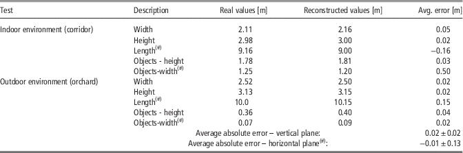
In order to prove the approach, two similar tests were conducted; the first in an indoor environment, a corridor, and the second in outdoor environment, an apple orchard, where the conditions change (due to wind). In both cases the reconstructed shapes were measured and compared to real measures for different objects with different sizes; windows for indoor, tree trunks for outdoor environment. In addition, because the vertical readings need to be placed at precise position, the data regarding cumulative length and intermediate distance between scans is considered as well as scene width and height. Table 1 summarizes the results.
Two different tests (indoor/outdoor environment) depicting real and reconstructed dimensions. Rows marked with (#) correspond to measurements from horizontal (SLAM supported) LIDAR and others to vertically positioned LIDAR

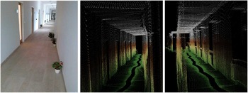
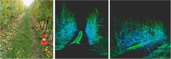
Figure 2 depicts the indoor environment and Figure 3 outdoor environment, both with part of the reconstructed 3D scene. Figure 2 clearly depicts objects from the scene and Figure 3 shows a real image of apple orchard and its 3D reconstruction from two slightly different viewpoints. The centre image clearly shows the space between the apple rows, while the right image distinct tree trunks (clusters of voxels in lower right side of an image).
Indoor environment – a corridor. The left image depicts a real scene, while image in the centre and on the right depict their representation in 3D space.

Outdoor environment - apple orchard. The left image depicts a real image, while in the centre and on the right it shows their representation3D reconstruction.

The tests were conducted while the robot was driving at roughly 0.5 m/s with the error rate of 0.015 m±0.03 m for vertical and −0.03 m±0.29 m for horizontal plane when comparing real to reconstructed dimensions. On average the error rate for estimating metric data in indoor environment was 0.02 m±0.02 m (or −0.11 m±0.08 m for horizontal and 0.03 m±0.015 m for vertical plane) and −0.01 m±0.13 m (or 0.09 m±0.01 m for horizontal and 0.01 m±0.03 m for vertical plane). The error rate is a bit higher for horizontal plane as it accumulates over time. The average errors (0.02 m and −0.01 m) are comparable, while the standard deviation is bit higher for outdoor environment due to changing silhouette and the speed the LIDAR is taking measurements vs the traveling speed of the robot.
In setup from Figure 1 the horizontal scanner takes scans at a higher level as the robot height. These cases no problems as far as the SLAM algorithm is concerned. It measures the distance to the walls (indoor) and tree trunks (outdoor). If it is to be used to detect the obstacles in from of the robot as well, the position of the two LIDARs could be switched or the horizontal scanner could be mounted at an angle, for instance at 45°.
Conclusions
This work summarises and evaluates an approach to reconstruct a 3D scene by using two 2D LIDAR sensors mounted vertically and horizontally. Similar results could be achieved by using a multi-channel 3D sensor. The advantages of the proposed solution are that this kind of setup is more economical (around 3- to 4-time less expensive) and it provides a higher degree of detail. The only real drawback is the method how it captures the details, as it has to pass each object instead of detecting it a couple of meters ahead like the multi-channel LIDAR sensor does.
To combine the readings by using two LIDAR sensors the data relative to the robot’s position must be available, which can be determined by using a SLAM algorithm. For this we used our own approch that is more efficient than other known solutions when working in outdoor environment where part of the scene could change due to outdoor forces.
The results show that the proposed approach is good enough for some applications, with the error rate of 0.015 m±0.03 m for vertical and −0.03 m±0.29 m for horizontal plane. To improve the results LIDAR sensors with higher resolution are suggested and slower robot driving speeds, with possible switch of LIDAR positions to enable the robot to detect obstacles in front of the robot.