Introduction
A lot of research has been carried out, exploring mmWaves for implementing the fifth-generation (5 G) communication system. Despite the merits mmWave provides, due to some major limitations like high absorption of waves as well as high path loss, sub-6 GHz band is more appropriate to realize 5G systems [1–Reference Niu, Li, Jin, Su and Vasilakos3]. The 5G wireless communication demands requirement of faster data transmission as well as better reliability, which can be accomplished using multiple input multiple output (MIMO) systems [Reference Chen and Zhao4], hence making it an integral part of 5G communication systems. For an antenna system to cater long distance transmission and to reduce path loss, a high-gain feature is must. In recent literature, various antennas have been developed to enhance the overall gain of system [Reference Wang, Cheng, Luo, Chen and Wu5,Reference Sun, Yang, Wang, Cheng, Luo, Chen and Li6]. Due to an increase in congestion or traffic in sub-6 GHz band, because of increasing active users, cognitive radios (CRs) are playing a key role in largely mitigating the issue [Reference Nguyen-Trong, Piotrowski and Fumeaux7,Reference Petosa8]. Therefore, antennas integrated with MIMO-CR feature are need of the hour. This could be achieved by designing smarter antennas and making them hybrid reconfigurable, in which their characteristics, such as pattern, polarization, frequency, gain, or bandwidth (BW), can be electronically adjusted by various means. For achieving reconfigurable behavior, we can either use conventional bandpass (BP) filters along with PIN diodes (PDs) to switch between various fixed discrete and fixed states for different applications [Reference Fakharian, Pezaei, Orouji and Soltanpur9, Reference Deng, Hou, Zhao and Guo10] or we can use varactor diodes (VDs) for continuous tuning of working states [Reference Qin, Wei and Guo11, Reference Tang, Wen, Wang, Li and Ziolkowski12]. The latter is obviously more acceptable for any random environment. A BW and frequency reconfigurable antenna (RA) is an appropriate choice for the application of CR or any frequency tunable wireless systems, as different working BWs are required for different application scenarios. Some of the RAs, having varied operating BWs, are listed in literature. In [Reference Cai, Li, Yin, Gao, Hu and Zhao13,Reference Krishna, Madhav, Anilkumar and Reddy14], the BW is varied from narrowband (NAB) to NAB, which may not be suitable for wideband (WB) communication operations. In [Reference Qin, Wei and Guo11, Reference Nguyen, Bui, Narbudowicz and Nguyen-Trong15,Reference Hussain, Ghaffar, Naqvi, Iftikhar, Anagnostou and Tran16], WB to NAB BW reconfiguration is successfully achieved. In [Reference Mansoul and Ghanem17, Reference Mansoul, Ghanem, Hamid, Salonen and Berg18], BW RA is proposed to have a fixed minimum frequency of operation, keeping the maximum frequency variable; in this way, overall BW of operation is adjusted. In [Reference Zang, Li, Ma, Yang and Xiong19], the BW reconfigurability is achieved using a monopole radiator as well as cascading of BP structures using a complex switching methodology. In [Reference Alqurashi, Kelly, Wang, Crean, Mittra, Khalily and Gao20], a liquid-metal-based BW RA is designed to obtain an ultra-wideband (UWB) mode and a NAB as well as improve back radiation by altering the defected ground configuration through liquid metal. A hybrid RA is presented in [Reference Nikam, Kumar, Baidya and Ghosh21], achieving pattern and BW tunability. Two different modes of operation are obtained using PDs. A λ/8 stub structure is used along with a feedline to vary the overall BW. In [Reference Hussain, Sharawi and Shamim22–Reference Sharjeel, Mansoor, Umer and Xiongwen24], the tuned operating bands achieved are shifted from the primary band of antenna (i.e., when all active elements are OFF), which could not be considered as a true BW RA. Hence, the tuned band should be within the primary operating band.
In almost all the reported literature, unexplored areas include a RA with both passband (PB) and notch band (NB) tunability with a large tuning range (TR), showing good gain (above 5–6 dBi) and continuous tuning with MIMO functionality.
In this work, an antenna system with frequency reconfiguration in both PB and NB with a wide frequency tuning range and BW reconfiguration in PB response was designed. Further, the antenna was extended to a 2-port MIMO structure in order to achieve better data rates and improve reliability of the overall system. Various MIMO parameters were analyzed for better performance validation. The structure was transformed into a two-element array to achieve better gain performance in the whole operating band. PDs and VDs are both used in the proposed work. PDs are used for switching between three modes (WB, tunable PB, and NB), and VDs for continuous tuning of frequency and BW in both PB and NB. Finally, TNN algorithm is applied to predict the optimum BW, for the first time, as per authors’ knowledge, for PB characteristics of proposed antenna.
Further, antenna configuration is central to any wireless network, requiring straightforward methods for parameter design and optimization. Yet, recent advancements such as miniaturization and increasingly complex antenna parameters have prolonged the time needed for high-frequency simulations. Consequently, leveraging machine learning (ML) has become the standard solution. Over the past few years, ML and artificial neural networks have emerged as robust frameworks for both designing and refining microwave components. Their use in a variety of microwave circuits and antenna systems, from modeling to optimization, has delivered significant improvements in performance and efficiency. Moreover, these approaches have notably shortened development cycles [Reference Singh and Yadav25,Reference Singh and Yadav26]. Therefore, in this work, various input parameters have been utilized to predict the percentage bandwidth of the antenna. The designed BW and frequency reconfigurable MIMO antenna are suitable for next-generation smart wireless applications like cognitive radio, etc.
Structural layout of DR-based antenna
For a better understanding of the design flow, adopted to create the proposed DR-based MIMO BW and frequency RA array design, and its working, this section is divided into sub-sections, which are: single element antenna design, two element antenna array configuration, RA array configuration, and two-port MIMO RA configuration.
Single element antenna design
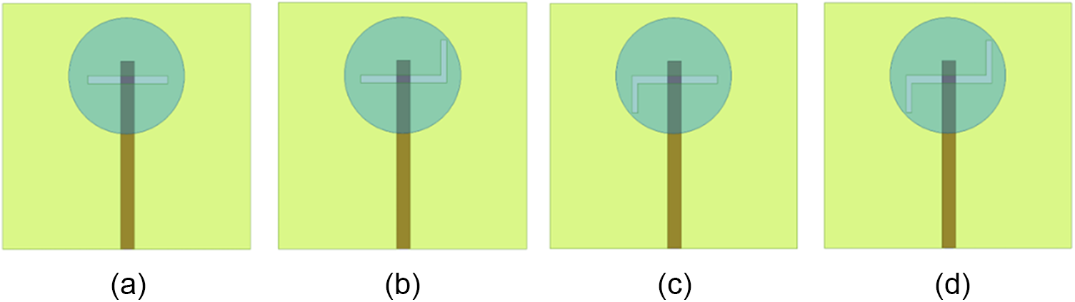
The first step in constructing a BW and frequency reconfigurable MIMO antenna array is designing its unit element or antenna with a single-element radiator. A Schematic of unit element antenna is shown in Fig. 1. Cylindrical resonators are used as the primary radiator made of alumina (ceramic) material, having  ${\varepsilon _r}$ = 9.8 with radius and height as 12.8 and 5 mm, respectively. Aperture coupling is used to excite the ceramic radiators. Initially, a horizontally placed rectangular aperture is designed having dimensions 17.7 × 1.75 mm2. Further, two vertically oriented side slots are etched orthogonally to rectangular slot, leading to a stair-shaped aperture as displayed in Fig. 1. This unit element antenna achieves a wide impedance bandwidth from 4.79 to 5.92 GHz. To analyze the reason for achieving a wider frequency band of operation, the S11 curve and electric field variations of different modification steps involved in the finalization of single-element antenna design are displayed. First of all, it can be confirmed from Fig. 3 that complete radiation is due to cylindrical resonators, as the configuration having only an aperture, excited using a line feed, is not resonating properly. Apart from this, E-field and S-parameter variations of four different configurations (Ant. 1,2,3,4) are also displayed in Fig. 3. All three antenna configurations are depicted in Fig. 2(a,b,c,d).
Schematic of a single-element antenna for array design with key parameters and components.

Schematic diagram of (a) Ant. 1, (b) Ant. 2, (c) Ant. 3, and (d) Ant. 4.

S11 and E-field distribution for all four antenna configurations.

In antenna 1, a horizontally oriented rectangular aperture is designed along with cylindrical DR and line feed. As is obvious, this structure produces HEM11δ mode field in the cDR with (-ve) x-oriented field component, which is because the rectangular aperture acts as a magnetic dipole placed horizontally [Reference Mongia and Bhartia27].
As the effective permittivity  $({\varepsilon _{eff}})$ and effective height
 $({H_{eff}})$ (cDR + substrate combined system) play a vital role in characterizing the behavior of the designed antenna, they can be formulated as given in [Reference Sharma, Das, Gupta and Gangwar28] using the following equations:
 \begin{equation}{H_{eff}} = H + {\text{ }}{H_S}\end{equation}
 \begin{equation}{\varepsilon _{eff}} = {\text{ }}\frac{{{H_{eff}}}}{{\frac{H}{{{\varepsilon _{rCDRA}}}} + \frac{{{H_S}}}{{{\varepsilon _{rSub}}}}}}\end{equation}
where  ${\varepsilon _{rCDRA}}$,
 ${\varepsilon _{rSub}}$ are the relative permittivities and
 $H,{\text{ }}{H_S}$ represents the heights of cDR and substrate, respectively. According to [Reference Sharma, Das, Gupta and Gangwar28], the equation used for the calculation of resonant frequency for the fundamental HEM11δ mode field is given as:
 \begin{align}&{f_{HE{M_{11\delta }}}} = \frac{{6.321 \times C}}{{2\pi \times R \times \sqrt {{\varepsilon _{r,eff}} + 2} }} \nonumber\\ & \left\{ {0.27 + 0.36 \left( {\frac{R}{{2 \times {H_{eff}}}}} \right) + 0.02{{\left( {\frac{R}{{2 \times {H_{eff}}}}} \right)}^2}} \right\}\end{align}
where R is radius of cDR,  $C{\text{ }}$ is speed of light,
 ${\varepsilon _{r,eff}}$ and
 ${H_{eff}}{\text{ }}$ are the effective relative permittivity and effective height of antenna system.
In antenna 2, a vertical slot is added above the horizontal slot as depicted in Fig. 2(b). This vertical slot produces an E-field in the (-ve) y-direction along with the (-ve) x-oriented field of the horizontal slot. Similarly, in antenna 3, the vertical slot placed below the horizontal aperture produces a (+ve) y-directed field component. These upper and lower vertical aperture slots behave as a magnetic dipole placed vertically [Reference Kajfez, Glisson and James29]. Finally, in the 4th configuration, by combining all three aperture structures, a resultant electric field oriented at 45° angle from the x-axis is obtained, showing HEM11δ mode fields. The individual close resonances produced by the horizontal as well as two vertical aperture slots, as visible from the S11 variations in Fig. 3, are coupled together to produce a WB response. The phenomenon responsible for this behavior is “mutual resonance” or coupling resonance, which improves the impedance matching of the overall structure, generating a WB [Reference Targonski, B.Waterhouse and Pozar30].
Two-element antenna array configuration
Before designing the antenna array structure, isolation among the two antenna elements is discussed. The gap between the centers of the two radiating elements is kept at 48 mm. No power divider arrangement is used at this stage, and the two antenna elements are fed by separate ports, which are depicted in Fig. 4(a). The S-parameter curves of the aforementioned configuration are displayed in Fig. 4(b) over the operating BW. It shows that the isolation among the ports is better than 25 dB value over almost the entire frequency band [Reference Kumar and Chaudhary31]. Hence, the 50 mm gap between the two radiating elements is chosen as a reference for the proposed array geometry. In order to design the 2-element array configuration, a 3-dB power divider has been incorporated with a simplified microstrip feeding network. A λ/4 impedance transformer is utilized in the feed structure [Reference Balanis32]. Figure 5 displays the antenna array configuration. This array antenna is designed on a commercially available FR-4 epoxy substrate with an electrical relative permittivity  $({\varepsilon _r}){\text{ }}$of 4.4 and loss tangent (tan δ) of 0.02. Dimensions for this configuration are chosen as 54.25 × 105 × 1.6 mm3. It is necessary to mention that DR and aperture dimensions are the same for both elements, as well as in every configuration. Figure 6(a) shows the comparative S11 parameter curve of the array structure and the unit element configuration. It can be observed from it that there is a close approximation between the S11 variations. Figure 6(b) shows the gain comparison between the 1 × 2 array structure as well as single radiator structure. The figure shows that the simulated gain value for the antenna array structure is nearly 2.5–3 dBi more, as compared to the single element configuration in most parts of the operating band. This happens due to the constructive interference of the radiation among the 2 elements, leading to a more directional pattern [Reference Gupta, Sharma, Das, RK and Khalily33].
(a) Geometrical layout for isolation check between the two radiating elements for array design, and (b) S-parameters versus frequency curve.

A 1 × 2 array geometry with 3-dB power divider line.

(a) Comparative S11, and (b) Gain for single radiator geometry and array design.

(a) Bandpass and (b) Bandreject filter structures without diodes and biasing and their S-parameter curves, (c) Reconfigurable bandpass, (d) Bandreject filter design, (e, f) Single port reconfigurable filter + antenna array layout with biasing circuit for diodes and (g, h) S11 response of structures shown in (c, d), respectively, and surface current distribution for (i) All diodes OFF, PB mode at VD cap. (j) 0.55 pF, (k) 1.18 pF, (l) 9.01 pF and NB mode at VD cap, (m) 0.72 pF, and (n) 1.18 pF.

Reconfigurable 1 × 2 array antenna configuration
This section describes the details of the frequency and BW reconfigurable two-element array antenna with three different modes of operation. In the array structure, which was already discussed in the previous section and is displayed in Fig. 5, some modifications have been incorporated within the feed network so as to adjust the lumped elements and resonating structures for frequency and BW tuning in the overall structure. This can be visualized from Fig. 7(e,f). Before integration of designed filters in the proposed array structure, their S-parameter characteristics, with and without diodes and biasing, are separately studied and is depicted in Fig. 7(a,b,g,h). The layout of reconfigurable PB and NB filters are illustrated in Fig. 7(c) and 7(d), respectively, at different capacitance values (which corresponds to a reverse bias voltage, applied in the measurement process) whereas filters without lumped elements are depicted in Fig. 7(a,b). In order to achieve a NB, a square ring-shaped resonator structure is attached in shunt to the feeding network, which behaves as an LC tank circuit. By altering the dimensions of the ring, L and C can be varied, which will further alter the resonant frequency and BW. Again, to accommodate the PB response in the overall structure, two separate dual square split ring type resonating structures are appended in shunt to the feeding network along with the NB structure. The dimensions of the two separate resonating structures are chosen to be slightly different to ensure that the notch frequencies of these resonators are also different, but not very far apart from each other. This difference is responsible for the BW of the PB response [Reference Alam, Thummaluru and Chaudhary34], which will be further exploited using VDs to achieve BW reconfigurability. All these modes are combined into the overall structure with the help of various PDs (S1–S12) and VDs (VD1–VD12). Out of the three basic modes of operations, the first one is the WB mode under which sensing could be done to further allocate some band to any particular node working for some wireless applications. In this mode, all the switches or PDs (S1–S6) are in OFF state. In mode 2, switches S1, S3, S4, and S6 are in ON state while S2 and S5 are in OFF state. This mode shows the PB response, due to the additional resonating structures connected in shunt. VD1, VD2, VD4, and VD5 being in active state, are used to tune the BW and frequency of the overall structure as VDs manipulate the dimensions of the resonating structure i.e. outer ring which shifts the frequency and also alters the BW because the inner ring resonant frequency is being fixed which varies the separation between the NB resonant frequency of the two structures.
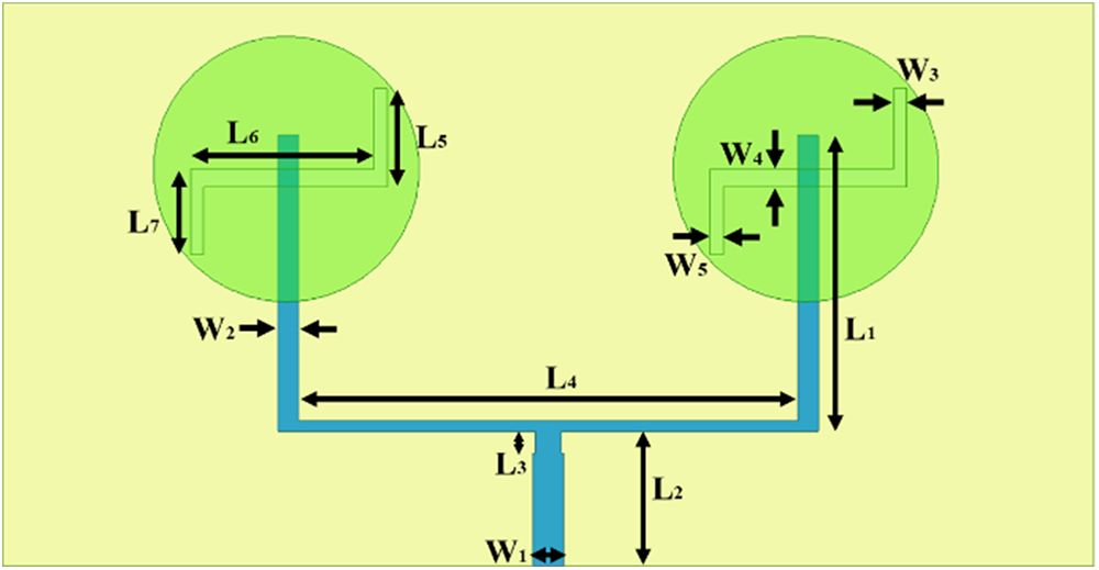
In mode 3, switches S2 and S5 are ON while S1, S3, S4, and S6 are OFF. This mode shows NB response due to the square ring open-loop structure connected in shunt with the feedline, acting as an LC tank circuit. Again, the dimensions of the ring are exploited using VD3 and VD6, producing tunable NB [Reference Alam, Thummaluru and Chaudhary34]. For practically applying the ON/OFF states of switches, a biasing circuit is designed. A biasing voltage diagram is shown in Fig. 8(a). For brevity, the switching of only one feeding network is shown in the figure, as the diode arrangements are identical for all the feeding networks. For mode 1, as switches S1, S2, S3 are all OFF, to achieve this, biasing voltages V1 is set at 0 V and V2, V3, V4 at high (5 V). The remaining can take any voltage value. For mode 2, switches S1 and S2 are ON and S3 is OFF. Here, V1 is set at 5 V, V2, V3 at 0 V (ground), and V4 at a higher voltage than V1 (10 V), while V7 can be set at any value. Also, V5 and V6 control the corresponding VDs for tuning the frequency and BW. For mode 3, S1 and S2 are OFF, and S3 is ON. For this to happen, V1 is set at 5 V, V2, V3 at a higher voltage than V1 (10 V), and V4 at 0 V, whereas V5 and V6 can be any value. V7 voltage controls the VD for tunability. This voltage-controlling operation is the same for each element of the array structure and finally, the MIMO configuration. Overall working of the antenna can be visualized from Table 1 shown. For mode 1, when all PDs and VDs are OFF, we get a fixed wide BW (BW 1), which can be used for spectrum sensing CR application. For mode 2, when PDs S1, S3, S4, S6 and VDs VD1, VD2, VD4, VD5 are ON, we get a tunable PB BW and frequency, going from a WB to NAB BWs (when VD reverse bias voltages are varied), utilized for communicating interweave CR operations where different application scenario needs different BWs for efficient operation. For mode 3, when PDs S2, S5 and VDs VD3 and VD6 are in ON state, we obtain tunable NB states, which rejects some portion of the spectrum (variably) and is applicable for underlay CR applications, which needs to reject the secondary user communication when it transmits above a certain threshold. Figure 7(i-n) shows the surface current distribution on feedline of proposed 1 × 2 array antenna for different modes of operation. For case 1, when all diodes are OFF, maximum current flows in the main branch of feedline and does not pass through the resonant ring structures placed in shunt with main arm. For cases 2 and 3, surface currents support tunable PB and NB response modes respectively. For this case, the maximum current bifurcates into open loop resonant structures added in parallel to main feeding arm. Further, for different capacitance values, the current value varies which manipulates the matching as well as provides shifting of resonant frequency. The optimized dimensions of the proposed structure are given as: L = 108.12, W = 105, R = 12.8, H = 5, H S = 1.6, L 1 = 28.5, L 2 = 13, L 3 = 2.1, L 4 = 48, L 5 = 9.5, L 6 = 17.65, L 7 = 8.25, L 8 = 7.8, L 9 = 5.25, L 10 = 2.9, L 11 = 2, L 12 = 2.55, L 13 = 1.4, L 14 = 2.55, W 1 = 3, W 2 = 2, W 3 = 1.25, W 4 = 1.75, W 5 = 1.25, W 6 = 0.4, W 7 = 0.2, and W 8 = 0.5 (units in mm).
(a) Diode bias voltage-controlling diagram, and (b) DC biasing circuit, PIN diodes in (c) ON state, (d) OFF state, and (e) Varactor diode equivalent circuit diagram.

Lumped elements (PD, VD) switching and tuning configurations for different modes of operation

Equivalent model of the diodes and biasing circuit
The RF PDs and VDs are loaded onto the feedline of the antenna in order to achieve frequency and BW tunability as well as switching among various modes of operation. The appropriate arrangement of the PDs and VDs to select different current paths is depicted in Fig. 7(f). The selected PDs and VDs are from Skyworks Inc., having model no. SMP 1345-079LF and SMV 1247-079LF, respectively. These diodes are chosen as per the frequency range of the designed antenna and work well in terms of switching and tuning performance. The equivalent model used for the PD and VD consists of a DC-blocking capacitor (C d), a current limiting resistor (R c), as well as RF chokes (L R), which is displayed in Fig. 8(b). C d blocks the biasing current flow inside the RF port, whereas L R allows the DC flow while blocking the RF current traveling. The optimal values for C d and L R are 3.6 pF and 0.4 nH, respectively. The value for R c is chosen to be 2.1 kΩ. The SMD PD used in the design works in 2 states, i.e., ON and OFF. As per the datasheet [35, 36], in the ON state of the diode, a voltage drop of 0.89 V occurs across it with 10 mA of forward current running through. Meanwhile, the diode works under reverse bias conditions in the OFF state. Practically in the ON state, PDs can be modeled as a series combination of R ON (2.1 ohm) and L P (0.4 nH), whereas in the OFF state, as a parallel combination of R OFF (2.1 kohm) and C OFF (0.15 pF) in series with L P. The equivalent circuit for both states is depicted in Fig. 8(c,d). However, for simplicity in the simulation process, only R ON and R OFF are used to work in the ON and OFF states of the PDs, respectively, which could be a possible reason for the variation in S11 simulated and measured outcomes for different modes. The VD is modeled as a series combination of R S (2.1 ohm), L S (0.4 nH), and C J varying from 0.55 pF to 9.01 pF, which is evaluated referring to the datasheet available. The equivalent circuit is depicted in Fig. 8(e). To switch between different modes as well as tuning of frequency and BW, seven different biasing voltages are applied at various nodes denoted by V1–V7. PDs and VDs are controlled using these voltages.
This bias-voltage-controlling circuit is depicted in Fig. 8(a) which is already explained in the previous section.
2-Port MIMO reconfigurable antenna array configuration
After the design of a single-port 2-element RA array, it is further extended to a two-port MIMO structure in order to suppress the multipath fading effect. This could be designed basically in three ways, one is by placing the ports parallelly or anti-parallel (mirror structure), or by orienting them orthogonally. Different orientations of MIMO antenna elements provide specific advantages when implemented. Parallel orientation provides optimum spatial efficiency and enables coherent processing, orthogonal configuration obtains maximum isolation and channel independence, while antiparallel arrangement facilitates beam control, directional selectivity, as well as improved isolation [Reference Sharma, Tiwari, Singh, Kumar and Kanaujia37,Reference Nadeem and Choi38]. Hence, as per the application requirement, any of the configurations could be selected. Antiparallel orientation provides 180° phase opposition due to a mirrored arrangement while maintaining the geometric symmetry [Reference Sharma, Tiwari, Singh, Kumar and Kanaujia37]. This arrangement generates counter-propagating surface currents that naturally cancel mutual coupling components through destructive interference [Reference Nadeem and Choi38]. This configuration is also capable of generating a low envelop correlation coefficient (ECC), which is essential for effective spatial diversity [Reference Upadhyaya, Sorathiya, Al-shathri, Shafai, Patel, Pandya and Armghan39]. In this particular work, the anti-parallel configuration is selected and is displayed in Fig. 9(a,b), which is the final proposed structure. Dimensions for this MIMO structure are 108.12 mm × 105 mm × 1.6 mm3. Figure 10(a–d) shows the simulated S11 parameter response for the WB mode as well as the tunability achieved in the PB and NB modes of the proposed 2-port MIMO reconfigurable array antenna. As per [Reference Petosa8], the formulation for total spectrum (TS) and tuning range (TR) is given as:
 \begin{equation}TS{\text{ }}\% = 2 \times \left( {\frac{{{f_{max}} - {f_{min}}}}{{{f_{max}} + {f_{min}}}}} \right) \times 100\end{equation}
 \begin{equation}TR{\text{ }}\% = 2 \times \left( {\frac{{{f_{high}} - {f_{low}}}}{{{f_{high}} + {f_{low}}}}} \right) \times 100\end{equation}
Geometrical layout: (a) Top view and (b) Perspective view of the proposed reconfigurable 2-port MIMO antenna array structure.

(a, b) Simulated S-parameters for wideband mode, (c) Partial BW and frequency reconfigurable states for PB response at different capacitance values, (d) NB frequency tunability and MIMO performance parameters, (e) ECC/DG, and (f) CCL/TARC.

Here, fmax and fmin are the maximum and minimum frequencies of operation of the proposed antenna, whereas fhigh and flow are the high and low resonance frequencies attained during the tuning.
Hence, the proposed array antenna achieves a simulated TS of 22.10% (4.83 GHz to above 6.03 GHz) and frequency TR of 18.15% (∼1.02 GHz range of tuning) for the PB response covering almost the whole wide sensing band of mode-1. The simulated BW reconfigurability is obtained with variation from 8.02% to 21.09%, with minimum BW occurring at higher capacitance values or lower applied reverse bias voltages. Figure 10(e,f) depicts the MIMO performance parameters for the proposed antenna structure. The correlation between individual antenna element’s patterns is depicted from envelope correlation coefficient (ECC) values. The overall gain of antenna system in a fading scenario is accounted for by diversity gain (DG) parameter. Using diversity techniques, these parameters can be obtained. Above mentioned MIMO parameters can be calculated as follows [Reference Sharawi40]:
 \begin{equation}ECC = {\text{ }}\frac{{{{\left| {S_{11}^*{\text{ }}{S_{12}} + {\text{ }}S_{21}^*{\text{ }}{S_{22}}} \right|}^2}}}{{\left( {\left( {1 - \left( {{{\left| {{S_{11}}} \right|}^2} + {\text{ }}{{\left| {{S_{21}}} \right|}^2}} \right)} \right)\left( {1 - \left( {{{\left| {{S_{22}}} \right|}^2} + {\text{ }}{{\left| {{S_{12}}} \right|}^2}} \right)} \right)} \right)}}\end{equation}
 \begin{equation}DG = 10{\text{ }}\sqrt {\left( {1 - {\text{ }}{{\left| {ECC} \right|}^2}} \right)} \end{equation}
To account for the maximum transmission rate that can be achieved for reliable message transfer through a channel, channel capacity loss (CCL) is calculated. CCL can be obtained using below mentioned formula [Reference Saurabh, Dubey and Meshram41]:
 \begin{equation}{\rho _{ii}} = 1 - {\text{ }}\mathop \sum \limits_{n = 1}^N \left| {S_n^*{S_{ni}}} \right|\end{equation}
 \begin{equation}{\rho _{ij}} = - {\text{ }}\mathop \sum \limits_{n = 1}^N \left| {S_n^*{S_{nj}}} \right|\end{equation}
 \begin{equation}{\varphi _R} = \left[ {{\rho _{ij}}} \right]\end{equation}
 \begin{equation}{C_{loss}} = - {\text{ }}lo{g_2}{\text{ }}det\left( {{\varphi _R}} \right)\end{equation}
Here,  ${\varphi _R}{\text{ }}$denotes the correlation matrix for receive antennas, and
 ${\rho _{ii}},{\text{ }}{\rho _{ij}}$ depicts correlation coefficients for all i,j where i and j are not equal. In a MIMO scenario instead of reflection coefficient we use another metric called as total active reflection coefficient (TARC), which accounts for both amplitude as well as phase properties of antenna’s S-parameters. It can be calculated as [Reference Sharawi40]:
 \begin{equation}TARC = {\text{ }}\frac{{\sqrt {\left( {\left( {{{\left| {{S_{11}} + {\text{ }}{S_{12}}{e^{j\theta }}} \right|}^2}} \right) + {\text{ }}\left( {{{\left| {{S_{21}} + {\text{ }}{S_{22}}{e^{j\theta }}} \right|}^2}} \right)} \right)} }}{{\sqrt 2 }}\end{equation}
Figure 10(e,f) signifies better diversity performance with all parameters showing values within the standard limits in the whole operating wideband. The proposed MIMO antenna with antiparallel orientation showed good ECC values below 0.02, DG close to 10 dB, CCL (magnitude) below 0.5 bits/sec/Hz and TARC below 0 dB within the obtained bandwidth.
Taguchi-NN approach for BW prediction
The process begins by simulating the antenna structure, from which performance data are extracted using electromagnetic (EM) simulation, Ansys HFSS. The resulting dataset typically includes four independent features and percentage bandwidth (% BW) prediction as a dependent feature. Any missing data in the dataset is handled through the mean approach, ensuring data quality and consistency. Initially, an extensive set of antenna-design parameters was assessed for its influence on percentage bandwidth. Because many of these variables were highly collinear, retaining them would have made the model complex without improving the performance. Accordingly, correlation-based feature elimination was applied which describes as whenever two parameters displayed an absolute Pearson correlation coefficient |ρ| approaching unity, the one less strongly associated with the target was discarded. This procedure produced a compact, interpretable feature set without compromising predictive accuracy. After consolidating the key features, the data are split into training, validation, and testing subsets with 70:15:15 split, respectively, providing a way to develop and then independently validate the predictive model. Feature scaling methods are subsequently employed to normalize or standardize the numeric ranges of different variables. Statistical tests such as the P-test, F-test, and ANOVA may be conducted to identify which parameters exert the most significant influence on antenna performance metrics, including bandwidth, resonance frequency, or gain. A Taguchi L9 design is then adopted to systematically tune the neural network’s hyperparameters (focusing on neuron count, learning rate, and batch size) while minimizing experimentation, as shown in Fig. 11. The neural network architecture illustrated in Fig. 12 represents a Taguchi Neural Network (TNN) framework designed to predict the % BW of an antenna using four key input parameters: varactor capacitance (CT) lower cut-off frequency ( ${F_L}$), higher cut-off frequency (
 ${F_H}$), and resonant frequency (
 ${F_R}$). Table 2 shows the list of independent variables with their specific range used to generate the dataset. Further the total number of dataset utilized were 3781.
The Taguchi L9 design flow.

Architectural framework of the proposed TNN algorithm.

Independent values used for the prediction

The model comprises an input layer, three hidden layers, and an output layer. The hidden layers are optimized using the Taguchi L9 orthogonal array, systematically varying hyperparameters, including the number of neurons ([5,10,15], [15,20,25], [25,30,35]), learning rate (0.0001, 0.001, 0.01), and batch size (2, 4, 6). This optimization ensures efficient training and minimizes the need for exhaustive parameter tuning. Further the performance metric of each trial in L9 taguchi methods is illustrated in Table 3.
The performance obtained in each trial of L9 Taguchi Network

Further, Table 4 compares the machine-learning models and shows that, although the TNN requires more computation time than the other models, it delivers superior performance metrics on test datasets.
Comparison among different ML models

The network’s output layer predicts the percentage bandwidth, capturing the non-linear relationship between the input features and the antenna’s performance. This TNN framework is a robust predictive tool for antenna design, significantly reducing the reliance on extensive simulations and accelerating the design optimization process. By efficiently modeling performance metrics, the framework supports rapid prototyping and enhances the overall efficiency of antenna development.
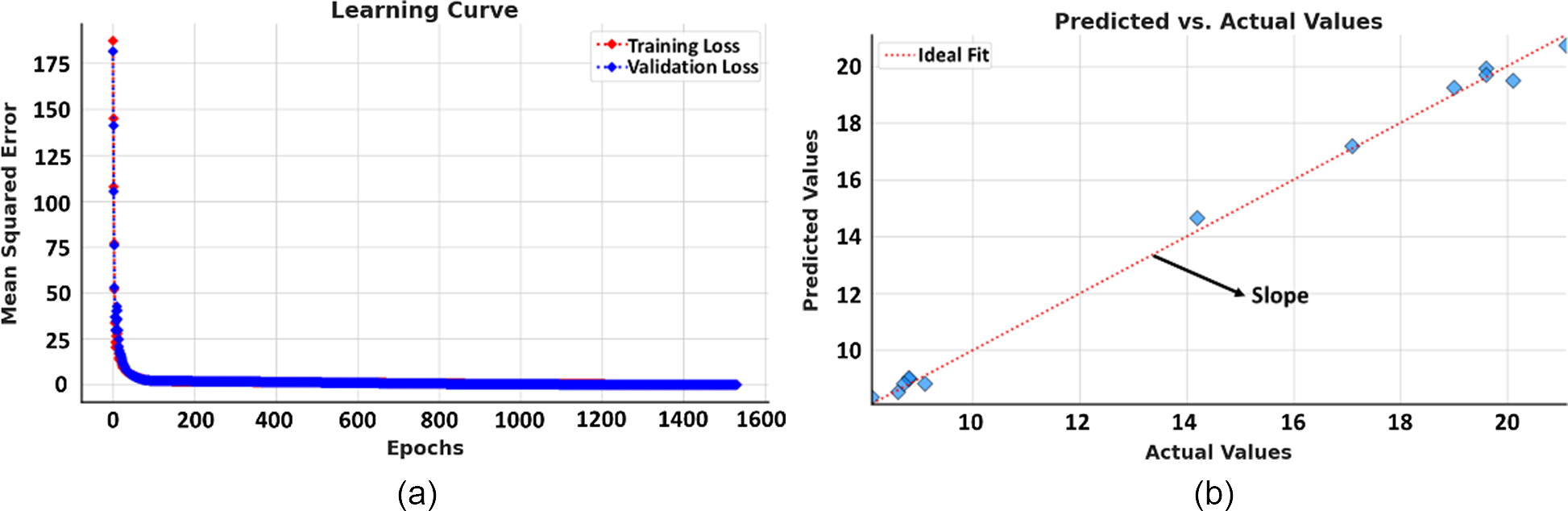
Further, Fig. 13(a) shows the model’s training and validation loss (mean squared error, MSE) over epochs. The steep decline in loss during the initial epochs indicates effective learning by the model. Both training and validation losses converge to a low value, suggesting the model is not overfitting or underfitting. The consistency between the two curves also reflects that the model generalizes well to unseen data.
(a) Training and validation loss (mean square error) over epochs and (b) Comparative curve of actual and predicted values of the target variable.

Also, Fig. 13(b) illustrates a scatter plot that compares the model’s predicted values against the actual values of the target variable. The red dashed line represents the ideal fit (perfect predictions where predicted values equal actual values). The points align closely with this line, indicating that the model achieves accurate predictions. The slope of the fit is near 1, confirming a strong linear correlation between predictions and actual values.
Further, the residual plot, as shown in Fig. 14(a), visualizes the difference between actual and predicted values (residuals) against the predicted values. The residuals are scattered around zero with no discernible pattern, which indicates that the model has captured the underlying structure of the data without systematic errors and a maximum error of 0.6 in percentage bandwidth. Figure 14(b) illustrates a histogram that represents the distribution of residuals, with a superimposed density curve. The residuals follow a roughly symmetric distribution centred around zero, suggesting that errors are randomly distributed. This is consistent with the assumption of homoscedasticity and indicates that the model’s errors are not biased toward under- or over-predictions.
(a) Plot of residuals (difference between actual and predicted values) vs the predicted values, (b) Distribution of residuals with superimposed density curve, and (c) comparative PDFs of predicted and actual values.

Finally, Fig. 14(c) compares the probability density functions (PDF) of the predicted and actual values. The overlap between the blue (actual) and orange (predicted) curves shows that the model’s predictions closely match the actual data distribution. This further demonstrates the accuracy of the model in capturing the underlying data patterns.
These plots collectively demonstrate the effectiveness of the neural network in modeling the target variable. The learning curve shows efficient training, the predicted vs. actual values and residual plots confirm strong accuracy and unbiased predictions, and the distribution plots highlight the alignment between the predicted and actual data distributions. The model appears well-tuned and reliable for the given task. Further, the algorithm for the Taguchi neural network is illustrated in Algorithm 1.performance as compared to others with respect to the provided features like tuning, MIMO feature, ML integration, etc.
Algorithm 1. Taguchi-NN Algorithm for the Percentage BW Prediction
Step 1: Initialize Parameters
• Select initial weights W
• Set number of epochs
Step 2: Design of Experiments (DOE) Using Taguchi Method
• Define levels L and factors F for the parameters
• Number of neurons in the hidden layer: {10,30,50}
• Learning rate: {0.0001,0.001,0.01}
• Batch size: {8,16,32}
• Generate orthogonal array OA for the experimental design using Taguchi L9
Step 3: Model Training
• for i = 1 to N do
- In practice, your code iterates over each combination of hyperparameters in the orthogonal array. For each combination C do:
• Set network parameters according to C
• Forward propagate X through the network
• Compute error E using loss function E(X,T,W)
• After each partial fit, you predict on both training and validation sets and compute MSE:
 \begin{equation*}MSE = {\text{ }}\frac{1}{n}\mathop \sum \nolimits^ {\left( {{y_{true}} - {y_{pred}}} \right)^2}\end{equation*}
• Update
$W \leftarrow W - \eta $ ∇E


• Evaluate performance metric (e.g., MSE) for C
Step 4: Optimization
• Select best combination C* with minimal error E
• Update final weights W* and biases based on C*
• Return W*
• Predict (X, W*)
Prediction
• Step 1: Forward Propagation
• Step 2: Return Predicted Values
X: Input data, T: Target (true) values, L: Levels of the parameters, F: Factors in the Taguchi method (neurons, learning rate, batch size), W: Weights of the neural network, η: Learning rate, N: Number of epochs (outer loop in the code), OA: Orthogonal array (from Taguchi method), C: One specific combination of hyperparameters from the Taguchi array, NN(X,W): Neural network forward pass, C*: Optimal combination of hyperparameters from Taguchi method, W*: The final weights after training with the best hyperparameters
In summary instead of testing every possible hyper-parameter combination (3 × 3 × 3 = 27 runs), the Taguchi method supplies a ready-made 9-run “orthogonal array” called L9 (33).
• Three columns = factors (here: hidden-layer neurons, learning rate, batch size).
• Three coded levels per column (e.g., neurons = 10, 30, 50, learning rate, and batch size).
• Nine rows of experiments chosen so the levels of any two factors appear in all independent pairings the same number of times (orthogonality).
Running the network on those nine well-balanced setups lets the model to estimate each factor’s effect on error and identify the best combination, while cutting training time by two-thirds compared with a full factorial search.
Measured outcomes
The fabricated prototype and measurement setup of the proposed BW and frequency reconfigurable 2-port MIMO antenna are shown in Fig. 15. For implementing the tunability, various lumped elements like PDs, VDs, surface mount device (SMD) resistors (2.1 Kohm), capacitors (3.6 pF), and inductors (0.4 nH) are soldered onto the proposed prototype. In the simulation process, the VDs are modeled as a series combination of forward resistance (2.1 ohm), ON state capacitance varying from 0.55 pF to 9.01 pF, and series inductance (0.4 nH) as referred from the LT spice diode modeling provided in the datasheet [35]. This is done in order to generate the voltage versus capacitance dataset for ML prediction by varying the diode parameters. The equivalent circuit of the VDs has already been discussed in previous sections. For switching of the PDs, a DC bias voltage is applied with a proper biasing circuit, consisting of a DC blocking capacitor and a series R-L circuit working as an RF choke, as discussed earlier. The S-parameters are measured using Agilent N5247A: A.09.90.02 vector network analyser (VNA), whereas the gain and radiation pattern are measured inside the anechoic chamber using Amkom Horn Antenna (1–18 GHz frequency range) as the RF source or transmitter, keeping the transmitted power as 13–15 dBm. The VNA is calibrated using TRL method with 3.5 SMA kit for calibration. The measurement setup for the S11 is divided into six modes just for brevity. Mode-1 represents the mode when all the PDs are in OFF state. Modes-2,3,4 depicts the three PB frequency and BW reconfigurable states (only at 0, 3, and 8 V reverse bias voltages, respectively) out of the various tunable states. Mode-5 and -6 show the NB tunability at VD reverse bias voltages of 3 and 4.5 V, respectively. The measured S11 curves for all the modes are depicted in Fig. 16(a–c). In these figures, partial states are only displayed for brevity. For mode-1/sensing mode, the −10 dB impedance BW of greater than 1.52 GHz (4.98 GHz to above 6.5 GHz) is achieved after the measurement, as displayed in Fig. 16(a). The measured S21/isolation among ports 1 and 2 is well within the limits and is acceptable which as depicted in Fig. 17(a). The anti-parallel orientation configuration is exploited here. The proposed MIMO antenna showed a measured wide PB frequency tuning range of 20.36% (∼1.1 GHz range of tuning) and BW reconfiguration from 16.69% to 34.44%. The NB tunability achieved is 6.1%, rejecting the 3.2 GHz 5G band as well. Simulated and measured gain as well as simulated radiation efficiency of the proposed MIMO antenna, are shown in Fig. 17(b). Gain and radiation pattern of the proposed structure are measured for the 0 V/C max condition. The measured gain is above 7 dBi in the whole operating band with a peak gain of 11.03 dBi. The measured gain is showing better results as compared to the simulated one, which is a rare thing but can be theoretically possible, mainly due to the real-world effects or the testing conditions that were not captured in the simulated model. The proposed antenna shows radiation efficiency greater than 60%, almost within the whole wide operating band, with peak efficiency greater than 70%. The measured E/H co- and cross-polarization radiation pattern at two different frequencies, i.e., 5.75 and 6 GHz within the sensing wideband is depicted in Fig. 18(a,b). The co-polarization radiation pattern shows consistent behavior at both the frequencies which is an advantageous feature. Also, it can be inferred from the figure that the co-polarization behavior dominates by more than 10 dB value in both E/H planes from the cross polarization for both frequencies. The E plane pattern shows close to omni directional radiation pattern for the sensing mode. Table 5 compares the proposed antenna with other state of the art works showing optimum
Fabricated prototype and measurement setup.

(a) Simulated and measured S11 parameter for mode 1, measured S11 for (b) Passband mode at 0, 3 and 8 V and (c) Notch band mode at 3, 4, and 5 V reverse bias voltages.

Simulated and measured (a) S-parameters for mode-1 (all diodes OFF), and (b) Gain, and simulated radiation efficiency of proposed reconfigurable MIMO antenna array.

Measured E/H plane co- and cross-polarization pattern at (a) 5.75 GHz and (b) 6 GHz.

Comparative performance of the proposed structure with previous reconfigurable antennas

Conclusion
A multi-mode wide to wide-to-NAB continuous BW and frequency reconfigurable MIMO antenna array is developed. The operating principle, stage-wise design procedure, and their result analysis are discussed. The open-loop resonating structures, along with varactor/PDs, play a key role in controlling the BW and operating frequency. The proposed antenna covers 5G sub-6 GHz (3.3–6.0 GHz)/Wi-Fi 6E (5.925–6.425 GHz)/Wi-Fi 5G (5.15–5.85 GHz) bands, i.e., 4.98–6.5 GHz, with a close to omnidirectional radiation pattern for mode-1 (sensing) operation, which is obvious. With the help of VDs, the continuous tuning of frequency (4.94–6.06 GHz) and BW (16.69%–34.44%) is achieved, which is further utilized to generate the dataset for the TNN model. Further, the presented evaluation metrics and visualizations collectively demonstrate the effectiveness and reliability of the TNN model. The learning curve confirms efficient training with minimal overfitting, while the alignment of predicted and actual values of percentage bandwidth illustrates the model’s accuracy. The residual plot and distribution indicate that the errors are unbiased and randomly distributed, with no systematic patterns or significant deviations. Furthermore, the strong overlap in the predicted and actual value distributions highlights the model’s ability to capture the underlying data structure accurately. Overall, the model is well-optimized and exhibits excellent predictive performance for percentage bandwidth prediction. Measured results confirm the suitability of the antenna for 5G-based cognitive communications.
Funding statement
Author, Anand Sharma, wishes to acknowledge the Council of Science and Technology, U.P. for giving the financial support to conduct this work successfully with notification No. CST/E&T/D-662 dated 01/08/2024.
Competing interests
The authors report no conflict of interest.

Yajush Rai born in Varanasi (U.P.), India, in 1993. He is a research scholar in the Electronics and Communication Engineering Department at Motilal Nehru National Institute of Technology Allahabad, Uttar Pradesh, India. He completed his Master’s degree (M.Tech.) in Electronics and Communication Engineering from the University of Allahabad, India in 2020 and his Bachelor’s degree in Electronics and Communication Engineering from Raj Kumar Goel Institute of Technology (R.K.G.I.T.) Ghaziabad, India in 2017. His research interests include dielectric resonator (DR) based antenna designs for sub-6 GHz 5G applications, DR-based reconfigurable antennas for cognitive radio applications, and antennas for imaging and sensing.

Suyash Kumar Singh received the B.Tech. degree in electronics and communication engineering from the Jaypee University of Engineering and Technology, India, and the M.E. degree in wireless communication from the Birla Institute of Technology, Ranchi, India. He has completed the Ph.D. degree with the Indian Institute of Information Technology, Allahabad, India. He has published several international journals. His research interests include microwave ablation antennas, passive and active microwave components, the use of machine learning, and artificial intelligence in microwave circuits/antennas.

Anand Sharma obtained Bachelor of Technology from Uttar Pradesh Technical University Lucknow in 2012, Master of Technology from Jaypee University of Engineering and Technology Guna in 2014, and Ph.D. in RF and Microwave from Indian Institute of Technology (ISM), Dhanbad in 2018. After that, he joined Government Engineering College Sonbhadra, U.P. as an Assistant Professor in Electronics Engineering Department and left the college in June 2019. Currently, he holds the position of Assistant Professor in the Department of Electronics and Communication Engineering, Motilal Nehru National Institute of Technology Allahabad, Prayagraj, U.P., India. He has published more than 60 articles in the International Journal (SCI Indexed) and also presented more than 40 articles in National/International Conferences. His area of research includes MIMO Antennas, Antenna for IoT Applications, Circularly Polarized DRAs, Ultra-Wideband and Super Wideband Antennas, Wearable Antennas, Antenna optimization using machine learning.

Smriti Agarwal was born in Lucknow (U.P.), India. She is currently working as an Assistant Professor in the Electronics and Communication Engineering Department at Motilal Nehru National Institute of Technology Allahabad, Uttar Pradesh, India. She has received her Ph.D. degree in millimeter wave imaging for target shape and fault identification from the Indian Institute of Technology Roorkee (IIT Roorkee), Roorkee, India. Mrs. Agarwal received a women scientist (WOS-A) fellowship from the Department of Science and Technology (DST) and a research intern fellowship from the Council of Scientific and Industrial Research (CSIR), India. Her research interest includes microwave and millimeter wave active imaging for target identification, non-destructive fault inspection, and millimeter wave planar antenna design.

Dr Rajeev Gupta is currently working as Associate Professor in the department of electronics and communication engineering of Motilal Nehru National institute of technology Allahabad, Prayagraj (India). He has completed his M.Tech. from Indian Institute of Technology Varanasi and acquired a degree of Ph.D. from MNNIT ALLAHABAD. His area of research in Antenna, RF, and Microwave Engineering.