1. Introduction
The motivation of this paper is to pave the way for obtaining sufficient and necessary conditions for the stability of non-linear Hawkes processes with inhibition. Hawkes processes are a class of point processes used to model events that have mutual influence over time. They were initially introduced by Hawkes in 1971 [Reference Hawkes10, Reference Hawkes and Oakes11] and are now used in a variety of fields such as finance, biology, and neuroscience.
More precisely, a Hawkes process
 $(N_t^h)_{t\in \mathbb{R}} = (N^h([0,t]))_{t\in \mathbb{R}}$
is defined by its initial condition on
 $(\!-\!\infty,0]$
and its stochastic conditional intensity denoted by
 $\Lambda$
, characterized by
 \begin{equation*} \Lambda(t) = \phi\bigg(\lambda + \int_{-\infty}^t h(t-s)\,N^h(\textrm{d}s)\bigg),\end{equation*}
where
 $\lambda >0$
,
 $h \colon \mathbb{R}_+ \to \mathbb{R}$
, and
 $\phi \colon \mathbb{R} \to \mathbb{R}_+$
are measurable, deterministic functions (see [Reference Daley and Vere-Jones4] for further details). The function h is called the reproduction function, and contains information on the behaviour of the process throughout time. In the case where
 $\phi$
is non-decreasing, the sign of the function h encodes for the type of time dependence: when h is non-negative, the process is said to be self-exciting; when h is signed, negative values of h can then be seen as self-inhibition [Reference Cattiaux, Colombani and Costa2, Reference Costa, Graham, Marsalle and Tran3]. The case where
 $h\ge0$
and
 $\phi=id$
is called the linear case. Considering signed functions h requires adding non-linearity by the mean of a function
 $\phi$
which ensures that the intensity remains positive. In this paper, we focus on the particular case where
 $\phi = (\!\cdot\!)_+$
is the rectified linear unit (ReLU) function defined on
 $\mathbb{R}$
by
 $(x)_+ = \max(0,x)$
.
Several authors have established sufficient conditions on h to ensure the existence of a stable version of this process. For signed h, [Reference Bremaud and Massoulie1] proved that a stable version of the process exists if
 $\|h\|_1<1$
, while [Reference Costa, Graham, Marsalle and Tran3] proved that it is sufficient to have
 $\|h^+\|_1<1$
, where
 $h^+(x)=\max(h(x),0)$
using a coupling argument. Unfortunately, this sufficient criterion does not take into account the effect of inhibition, captured by the negative part of h. Going further is difficult because non-linearity breaks the direct link between the function h and the probabilistic structure of the Hawkes process. Recent results have been obtained in [Reference Raad and Löcherbach14] for a two-dimensional non-linear Hawkes process with weighted exponential kernel, modeling the case of two populations of interacting neurons including both inhibition and excitation, and providing a criterion on the weight function matrix for stability exploiting the Markovian structure of the Hawkes process in that case. It is noteworthy that the stability condition [Reference Raad and Löcherbach14, Assumption 1.2] is similar to the case
 $\mathcal{R}_2$
of this paper, by reinterpreting the meaning of our parameters to correspond to those of the model described in [Reference Raad and Löcherbach14]. Our work focuses on a simpler process due to its discrete-time nature, yet the significance of our study lies in providing an almost complete classification of its asymptotic behaviour without requiring assumptions on the parameter values of the model.
In order to get an intuition on the results that we might obtain on Hawkes processes, we choose to consider a simplified, discrete analogue of those processes. Namely, we study an autoregressive process
 $(\tilde X_n)_{n\ge 1}$
with initial condition
 $(\tilde X_0, \dots, \tilde X_{-p+1})$
where
 $p \in \{ 1, 2, \dots \}$
, and such that, for all
 $n \geq 1$
,
 \begin{equation*} \tilde X_n \sim \mathcal{P}(\phi(a_1\tilde X_{n-1} + \cdots + a_p\tilde X_{n-p} + \lambda)),\end{equation*}
where
 $\mathcal{P}(\rho)$
denotes the Poisson distribution with parameter
 $\rho$
, and
 $a_1,\ldots,a_p$
are real numbers.
In the linear case (
 $a_1,\ldots,a_p$
non-negative, and
 $\phi(x)=x$
) these integer-valued processes are called INGARCH processes, and have already been studied in [Reference Ferland, Latour and Oraichi6, Reference Fokianos and Fried7], where a necessary condition for the existence and stability of this class of processes has been derived and can be written as
 $\sum_{i=1}^p {a_i}<1$
. Furthermore, the link between Hawkes processes and autoregressive Poisson processes has already been made for the linear case: the discretized autoregressive process (with
 $p = +\infty$
) has been proved to converge weakly to the associated Hawkes process [Reference Kirchner12]. Although this convergence has only been demonstrated in the linear case, i.e. with positive
 $a_i$
, it seemed valuable to us to understand the modifications induced by the presence of inhibition on the asymptotic behavior of these processes. An analogous discrete process has been proposed in [Reference Seol15] using an autoregressive structure based on Bernoulli random variables.
In order to explore the effect of inhibition, we consider signed values for the parameters
 $a_1,\ldots,a_p$
. In this article, we focus on the specific case of
 $p=2$
, so that our model of interest can be written as
 \begin{equation} \textrm{for all } n \geq 2, \quad \tilde X_n \sim \mathcal{P}((a\tilde X_{n-1} + b\tilde X_{n-2} + \lambda)_+),\end{equation}
with
 $a,b \in \mathbb{R}$
and
 $\tilde X_0, \tilde X_1 \in \mathbb{N}$
. (In this paper we will use the convention
 $0 \in \mathbb{N}$
.)
The most important result here is the classification of the process defined in (1). Note that complete characterization of the behaviour of this simple process is difficult due to the variety of behaviours observed. We prove that the introduction of non-linearity through the ReLU function makes the process more stable relative to its linear counterpart, in the sense that the parameter space
 $(a,b) \in \mathbb{R}^2$
for which the linear process
 $y_{n+1}=ay_{n}+by_{n-1}+\lambda$
admits a stationary version is strictly a subset of the parameter space for which the non-linear process admits a stationary version (see Appendix A). Our results also illustrate the complex role of inhibition, and in particular the asymmetric role of a and b associated with the range at which inhibition occurs. Our work suggests the existence of complex algebraic and geometric structures that are likely to play an important role in the more general case of a memory of order p. In order to obtain our results we use a wide range of probabilistic tools, corresponding to the variety of the behaviours of the trajectories of the process, depending on the parameters of the model.
2. Notation, definitions, and results
2.1. Definition and main result
Let
 $a,b \in \mathbb{R}$
and
 $\lambda > 0$
. We consider a discrete-time process
 $(\tilde{X}_n)_{n \geq 1}$
with initial condition
 $(\tilde{X}_0, \tilde{X}_{-1})$
such that the following holds for all
 $n\ge 1$
:
 \begin{equation*} \textrm{conditioned on}\ \tilde{X}_{-1},\ldots,\tilde{X}_{n-1}: \quad \tilde{X}_n\sim\mathcal{P}((a\tilde{X}_{n-1} + b\tilde{X}_{n-2} + \lambda)_+), \end{equation*}
where
 $(\!\cdot\!)_+$
is the ReLU function defined on
 $\mathbb{R}$
by
 $(x)_+ \;:\!=\; \max(0,x)$
.
As we said previously, some papers have already dealt with the linear version of this process: if a and b are non-negative, the parameter of the Poisson random variable in (1) is also non-negative, and the ReLU function vanishes. In this case, [Reference Ferland, Latour and Oraichi6, Proposition 1] states that the process is a second-order stationary process if
 $a+b<1$
. This weak stationarity ensures that the mean, variance, and autocovariance are constant with time.
Let us define the function
 \begin{align*} b_\textrm{c}(a) = \begin{cases} 1 & a \le 0, \\[5pt] 1-a & a\in(0,2), \\[5pt] -\dfrac{a^2}{4} & a\ge 2, \end{cases}\end{align*}
and define the following sets (see Figure 1):
 \begin{equation} \mathcal R = \{(a,b)\in\mathbb{R}^2\colon b<b_\textrm{c}(a)\}, \qquad \mathcal T = \{(a,b)\in\mathbb{R}^2\colon b>b_\textrm{c}(a)\}.\end{equation}
Our main result is the following.
Theorem 1. If
 $(a,b) \in \mathcal{R}$
, then the sequence
 $(\tilde X_n)_{n\ge0}$
converges in law as
 $n\to\infty$
.
If
 $(a,b) \in \mathcal{T}$
, then the sequence
 $(\tilde X_n)_{n\ge0}$
satisfies, almost surely,
 $\tilde X_n+\tilde X_{n+1}\underset{n\to\infty}{\longrightarrow}+\infty$
.
The partition of the parameter space described in Theorem 2. The green region corresponds to
 $\mathcal{R}$
, while the red region corresponds to
 $\mathcal T$
. The smaller figures are typical trajectories of the Markov chain
 $(X_n)_{n\ge0}$
for each region of the parameter space. In all the simulations, we chose
 $\lambda=1$
. The region delineated by the dashed triangular line corresponds to the region of parameter space for which the linear recurrence equation
 $y_{n} = ay_{n-1} + by_{n-2} + \lambda$
is bounded for all
 $n \in \mathbb{N}$
, for any given
 $y_0, y_1 \in \mathbb{R}$
. See Appendix A for more details.

This result derives from studying the natural Markov chain associated with
 $\tilde X_n$
that is defined by
 \begin{equation} X_n \;:\!=\; (\tilde X_{n}, \tilde X_{n-1}), \qquad n\ge0.\end{equation}
Before giving more details about the behaviour of
 $(X_n)_{n\ge0}$
, let us comment on Theorem 1. In particular, we stress that the condition for convergence in law is not symmetrical in a and b. More precisely, for any
 $a\in\mathbb{R}$
, the sequence
 $(\tilde X_n)$
can be tight provided that b is chosen small enough, but the converse is not true as soon as
 $b>1$
. This induces inhibition having a stronger regulating effect when it occurs after an excitation rather than before.
The question of the critical behaviour of the process on the boundary
 $\{b=b_\textrm{c}(a)\}$
remains open and presents a difficult question for further work.
2.2. The associated Markov chain
As mentioned, the main part of this article is devoted to studying a Markov chain
 $(X_n)$
which encodes the time dependency of
 $(\tilde X_n)$
. We rely on the recent treatment in [Reference Douc, Moulines, Priouret and Soulier5] for results about Markov chains. In particular, we use their notion of irreducibility, which is weaker than the usual notion of irreducibility typically found in textbooks on Markov chains (on a discrete state space). Thus, a Markov chain is called irreducible if there exists an accessible state, i.e. a state that can be reached with positive probability from any other state. Following [Reference Douc, Moulines, Priouret and Soulier5], we refer to the usual notion of irreducibility (i.e. every state is accessible) as strong irreducibility.
The transition matrix of the Markov chain
 $(X_n)_{n\ge0}$
defined in (3) is thus given for
 $(i,j,k,l)\in\mathbb{N}^4$
by
 \begin{equation*} P((i,j), (k,\ell)) = \delta_{i\ell}\frac{\textrm{e}^{-s_{ij}}s_{ij}^k}{k!},\end{equation*}
where
 $s_{ij} \;:\!=\; (ai+bj+\lambda)_+$
and
 \begin{align*}\delta_{ij} \;:\!=\;\begin{cases} 1 & \textrm{if}\; i=j, \\[5pt] 0 & \textrm{otherwise}.\end{cases}\end{align*}
In other words, starting from a state (i, j), the next step of the Markov chain will be (k, i) where
 $k \in \mathbb{N}$
is the realization of a Poisson random variable with parameter
 $s_{ij}$
. In particular, if
 $s_{ij} = 0$
, then the next step of the Markov chain is (0,i).
Since the probability that a Poisson random variable is zero is strictly positive, it is possible to reach the state (0,0) with positive probability from any state in two steps. In particular, the state (0,0) is accessible and the Markov chain is irreducible. Furthermore, the Markov chain is aperiodic [Reference Douc, Moulines, Priouret and Soulier5, Section 7.4], since
 $P((0,0),(0,0)) = \textrm{e}^{-\lambda} > 0$
. Note that strong irreducibility may not hold (see Proposition 2).
Recall the definition of the sets
 $\mathcal{R}$
and
 $\mathcal{T}$
in (2).
Theorem 2. Let
 $(a,b)\in \mathcal R$
. Then the Markov chain
 $(X_n)_{n\ge0}$
is geometrically ergodic, i.e. it admits an invariant probability measure
 $\pi$
and there exists
 $\beta > 1$
such that, for every initial state,
 $\beta^n d_\textrm{TV}(\operatorname{Law}(X_n),\pi) \to 0$
, as
 $n\to\infty$
, where
 $d_\textrm{TV}$
denotes total variation distance.
Let
 $(a,b)\in\mathcal T$
. Then the Markov chain is transient, i.e. every state is visited a finite number of times almost surely, for every initial state.
Theorem 1 is a simple consequence of this result. Indeed, in the case of
 $(a,b)\in\mathcal{R}$
, the convergence in law of
 $\tilde{X}_n$
simply derives from the convergence in law of
 $X_n$
since
 $\tilde{X}_n$
is the first coordinate of
 $X_n$
. In the transient case,
 $(a,b)\in\mathcal{T}$
, the result in Theorem 1 simply derives from the fact that
 $||X_n||_1\to_{n\to\infty}\infty$
almost surely.
The rest of the article is devoted to the proof of Theorem 2. We first focus on the recurrent case in Section 3, then on the transient case in Section 4. Throughout, we provide typical trajectories of the cases considered. For the sake of clarity we have plotted the realizations of
 $(X_n)_{n=0,\dots,N}$
by connecting its successive realizations. Unless otherwise stated, for coherence purposes we always set
 $X_0 = (0,0)$
and
 $\lambda = 1$
for our plots.
3. Proof of Theorem 2: Recurrence
In this section we prove the recurrence part of Theorem 2. The proof goes by exhibiting three functions satisfying Foster–Lyapounov drift conditions for different ranges of the parameters (a, b) covering the whole recurrent regime
 $\mathcal R$
.
3.1. Foster–Lyapounov drift criteria
Drift criteria are powerful tools that were introduced in [Reference Foster8], and deeply studied and popularized in [Reference Meyn and Tweedie13], among others. These drift criteria allow us to prove convergence to the invariant measure of Markov chains and yield explicit rates of convergence. Here we use the treatment from [Reference Douc, Moulines, Priouret and Soulier5], which is influenced by [Reference Meyn and Tweedie13], but is more suitable for Markov chains that are irreducible but not strongly irreducible.
A set of states
 $C\subset \mathbb{N}^2$
is called petite [Reference Douc, Moulines, Priouret and Soulier5, Definition 9.4.1] if there exists a state
 $x_0\in \mathbb{N}^2$
and a probability distribution
 $(p_n)_{n\in\mathbb{N}}$
on
 $\mathbb{N}$
such that
 $\inf_{x\in C}\sum_{n\in\mathbb{N}} p_n P^n(x,x_0) > 0$
, where we recall that
 $P^n(x,x_0)$
is the n-step transition probability from x to
 $x_0$
. Since the Markov chain
 $(X_n)_{n\ge0}$
is irreducible, any finite set is petite (take
 $x_0$
to be the accessible state) and any finite union of petite sets is petite [Reference Douc, Moulines, Priouret and Soulier5, Proposition 9.4.5].
Let
 $V \colon \mathbb{N}^2 \to [1,\infty)$
be a function,
 $\varepsilon\in(0,1]$
,
 $K<\infty$
, and
 $C\subset \mathbb{N}^2$
a set of states. We say that the drift condition
 $D(V,\varepsilon,K,C)$
is satisfied if
 \begin{equation*} \Delta V(x) \;:\!=\; \mathbb{E}_x [V(X_1)-V(X_0)] \leq -\varepsilon V(x)+K\boldsymbol 1_C,\end{equation*}
where
 $\mathbb{E}_x[\cdot] = \mathbb{E}[\,\cdot \mid X_0 = x]$
. It is easy to see that this condition implies the condition
 $D_g(V,\lambda,b,C)$
from [Reference Douc, Moulines, Priouret and Soulier5, Definition 14.1.5], with
 $\lambda = 1-\varepsilon$
and
 $b = K$
.
Proposition 1. Assume that the drift condition
 $D(V,\varepsilon,K,C)$
is verified for some V,
 $\varepsilon$
, K, and C as above, and assume that C is petite. Then there exists
 $\beta > 1$
and a probability measure
 $\pi$
on
 $\mathbb{N}^2$
such that, for every initial state
 $x\in \mathbb{N}^2$
,
 \begin{align*} \beta^n\times \sum_{y\in \mathbb{N}^2} V(y)|\mathbb{P}_x(X_n = y)-\pi(y)| \to 0, \qquad n\to\infty. \end{align*}
In particular, for every initial state
 $x\in \mathbb{N}^2$
,
 $\beta^n d_\textrm{TV}(\operatorname{Law}(X_n),\pi)\to 0$
as
 $n\to\infty$
, and
 $\pi$
is an invariant probability measure for the Markov chain
 $(X_n)_{n\ge0}$
.
Proof. As mentioned in Section 2.2, the Markov chain is irreducible and aperiodic. The first statement then follows by combining parts (ii) and (a) of [Reference Douc, Moulines, Priouret and Soulier5, Theorem 15.1.3] with the remark preceding [Reference Douc, Moulines, Priouret and Soulier5, Corollary 14.1.6]. The second statement follows immediately, noting that
 $V\ge 1$
.
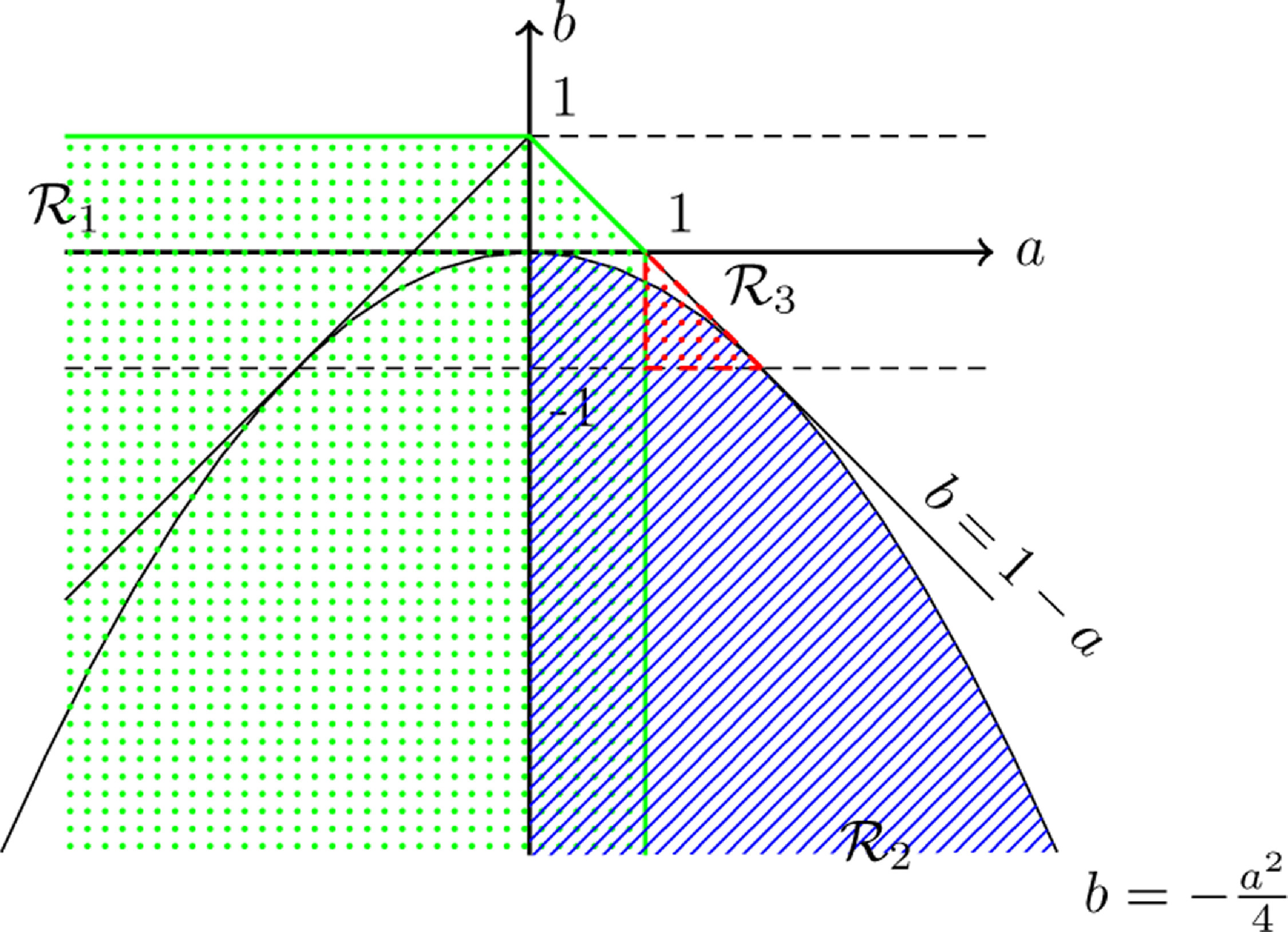
We consider separately the following ranges of the parameters:
 \begin{align*} \mathcal R_1 &= \{(a,b)\in \mathbb{R}^2\colon a,b < 1\textrm{ and }a+b<1\}; \\[5pt] \mathcal R_2 &= \{a>0\textrm{ and }a^2 + 4b < 0\}; \\[5pt] \mathcal R_3 &= \{1\le a<2\textrm{ and } {-}1 < b < 1-a\}.\end{align*}
We then have
 $\mathcal R = \mathcal R_1\cup\mathcal R_2\cup \mathcal R_3$
; see Figure 2.
Illustration of the three zones of parameters on which the proof of ergodicity will be carried.
3.2. Case
 $\mathcal R_1$

This case is the natural extension of the results that have been already proved for the linear process (see [Reference Ferland, Latour and Oraichi6, Proposition 1]).
Let
 $V \colon \mathbb{N}^2 \to \mathbb{R}_+$
be the function defined by
 $V ( i, j ) \;:\!=\; \alpha i + \beta j + 1$
, where
 $\alpha,\beta >0$
are parameters to be chosen later. Then
 $V ( i, j ) \geq 1$
for all
 $( i, j ) \in \mathbb{N}^2$
. We look for
 $\varepsilon > 0$
such that
 $\Delta V(x) + \varepsilon V(x) \leq 0$
except for a finite number of
 $x \in \mathbb{N}^2$
.
Let
 $\varepsilon > 0$
to be properly chosen later. Then,
 \begin{align*} \Delta V ( i, j ) + \varepsilon V ( i, j ) & = \sum_{k \in \mathbb{N}}\frac{\textrm{e}^{-s_{ij}}s_{ij}^k}{k!}(\alpha k + \beta i + 1) - (\alpha i + \beta j + 1) + \varepsilon(\alpha i + \beta j + 1) \\[5pt] & = \alpha s_{ij} + i(\beta - \alpha + \alpha\varepsilon) + j(\beta\varepsilon - \beta) + \varepsilon . \end{align*}
Note that
 $s_{ij} = 0$
or
 $s_{ij} = ai + bj + \lambda > 0$
. In both cases,
 $\Delta V + \varepsilon V$
is a linear function of
 $( i, j ) \in \mathbb{N}^2$
. We thus choose
 $\alpha, \beta$
such that the coefficients of
 $\Delta V + \varepsilon V$
are negative, so there will be only a finite number of (i, j) that satisfy
 $\Delta V ( i, j ) + \varepsilon V ( i, j ) \geq 0$
.
Let us first consider couples (i, j) such that
 $s_{ij}=0$
. According to the above, it is sufficient to have
 \begin{align*}\left\{ \begin{array}{ll} \beta - \alpha + \alpha\varepsilon < 0 \\[5pt] \beta\varepsilon - \beta < 0 \end{array} \right. \quad \Longleftrightarrow \quad\left\{ \begin{array}{ll} \beta < \alpha(1-\varepsilon) \\[5pt] \varepsilon < 1 \end{array} \right. \end{align*}
In what follows, we impose
 $\varepsilon <1$
.
If
 $s_{ij} = ai+bj+\lambda > 0$
, then
 \begin{align*}\Delta V( i, j )+ \varepsilon V ( i, j ) = i(\alpha a - \alpha + \beta + \alpha \varepsilon) + j(\alpha b + \beta \varepsilon - \beta) + \lambda \alpha + \varepsilon.\end{align*}
For the same reasons as before, it is sufficient to have
 $\alpha,\beta > 0$
such that
 \begin{align*}\left\{ \begin{array}{ll} \alpha a - \alpha + \beta + \alpha\varepsilon < 0 \\[5pt] \alpha b + \beta\varepsilon - \beta < 0 \end{array} \right. \quad \Longleftrightarrow \quad\left\{ \begin{array}{ll} \beta < \alpha (1 - a - \varepsilon) \\[5pt] \beta > \dfrac{\alpha b}{1-\varepsilon} \qquad\quad (\mbox{since } \varepsilon < 1) \end{array}\right.\end{align*}
Let
 $\alpha \;:\!=\; 1$
. With the above statements we thus want to choose
 $\beta, \varepsilon > 0$
such that
 \begin{align*}\left\{ \begin{array}{ll} \dfrac{b}{1-\varepsilon} < \beta < 1-a-\varepsilon, \\[5pt] \beta < 1-\varepsilon; \end{array} \right. \quad \textrm{i.e.} \quad \dfrac{b}{1-\varepsilon} < \beta < \min\{ 1-a-\varepsilon, 1 - \varepsilon\}.\end{align*}
Recall that
 $a+b<1$
, so it is possible to find
 $\varepsilon_0 \in (0,1)$
small enough that, for all
 $\tilde{\varepsilon} \leq \varepsilon_0$
,
 \begin{align*}\frac{b}{1-\tilde{\varepsilon}} < 1 -a-\tilde{\varepsilon}.\end{align*}
If
 $a \geq 0$
, then
 $\min\{1-a-\varepsilon, 1 - \varepsilon\} = 1 - a - \varepsilon$
and, since
 $a < 1$
, we can choose
 $\varepsilon \leq \varepsilon_0$
small enough that
 ${b}/({1-\varepsilon}) < \beta < \min \{ 1-a-\varepsilon, 1 - \varepsilon\}$
on one hand, and
 $1-a-\varepsilon > 0$
on the other hand. It is thus possible to choose
 $\beta > 0$
such that
 \begin{align*}\dfrac{b}{1-\varepsilon} < \beta < \min \{ 1-a-\varepsilon, 1 - \varepsilon \}.\end{align*}
If
 $a < 0$
, then
 $\min \{ 1-a-\varepsilon, 1 - \varepsilon \} = 1 - \varepsilon$
. Since
 $b<1$
, it is possible to set
 $\varepsilon \leq \varepsilon_0$
small enough that
 $b < (1 - \varepsilon)^2$
. Hence, we have
 ${b}/({1-\varepsilon}) < 1 - \varepsilon$
, so that it is possible to choose
 $\beta > 0$
that satisfies our constraints.
Note that
 $\Delta V( 0, 0 ) = \lambda > 0$
. Hence, with
 $\alpha, \beta, \varepsilon > 0$
chosen as above,
 $\Delta V( i, j )\le -\varepsilon V ( i, j )$
except for a finite number of states
 $( i, j ) \in \mathbb{N}^2$
. This proves that a drift condition
 $D(V,\varepsilon,C)$
holds for a finite set C, which yields the result.
3.3. Case
$\mathcal R_2$

In this section, we assume that
 $a>0$
and
 $a^2+4b<0$
. The Lyapounov function we will consider is the following:
 \begin{align*}\textrm{for all } ( i, j ) \in \mathbb{N}^2, \quad V ( i, j ) = \dfrac{i}{j+1}+1.\end{align*}
Before getting into the details, a remark about this function. While we initially discovered it by trial and error, it has an interesting geometric interpretation. As shown in Figure 3, for the case of
 $\mathcal R_2$
the macroscopic trajectories of the Markov chain tend to turn counterclockwise until they hit the j-axis and eventually get pulled back to (0, 0). This provides a heuristic understanding of why V should be a Lyapounov function. Indeed, it is an increasing function of the angle between the vector (i, j) and the j-axis, and therefore
 $V(X_n)$
should have a tendency to decrease whenever
 $X_n$
is far away from the j-axis.
An illustration of the case of
 $\mathcal R_2$
. Here, the parameters are
 $a = 3$
,
 $b = -2.5$
, and
 $N=1000$
. The red region indicates the set A of couples (i, j) such that
 $s_{ij}=s_{0i}=0$
.

We now turn to the details. We will need to distinguish the region A of the states (i, j) where
 $s_{ij}=0$
(shown in red in Figure 3):
 \begin{equation*} A \;:\!=\; \{(i, j) \in \mathbb{N}^2 \colon s_{ij} = 0\} = \{(i, j) \in \mathbb{N}^2 \colon ai+bj+\lambda \le 0\}.\end{equation*}
We have the following lemma.
Lemma 1. The set A is petite.
Proof. By the definition of A, we have
 $s_{ij} = 0$
for all
 $(i,j)\in A$
, and hence
 $P((i,j),(0,i)) = 1$
. Furthermore, for every
 $i\in \mathbb{N}$
, since
 $b<-a^2/4 < 0$
,
 \begin{align*} P((0,i),(0,0)) = \textrm{e}^{-s_{0i}} = \textrm{e}^{-(\lambda+bi)_+} \ge \textrm{e}^{-\lambda}. \end{align*}
It follows that
 $\inf_{(i,j)\in A} P^2((i,j),(0,0)) \ge \textrm{e}^{-\lambda} > 0$
, which shows that A is petite.
Lemma 2. There exists a finite set
 $C\subset\mathbb{N}^2$
and
 $\varepsilon\in(0,1)$
such that the drift condition
 $D(V,\varepsilon,K,A\cup C)$
is satisfied for some
 $K<\infty$
.
Proof. Since
 ${a^2}/{4}+b < 0$
, there exists
 $\varepsilon \in (0,1)$
small enough that
 \begin{align*}\frac{(a+\varepsilon)^2}{4}+b(1-\varepsilon)<0.\end{align*}
Consider
 $(i,j) \not \in A$
, and compute
 \begin{align*} \Delta V ( i, j ) + \varepsilon V(i,j) = \dfrac{(\varepsilon-1)i^2+bj^2+(a+\varepsilon)ij + L_1(i,j)}{(i+1)(j+1)}, \end{align*}
where
 $L_1(i,j)$
is a polynomial of degree 1. In the numerator we recognize a quadratic form, and as
 ${(a+\varepsilon)^2}/{4}+b(1-\varepsilon)<0$
, this quadratic form is negative definite. Thus, there are only a finite number of
 $(i,j) \not \in A$
such that
 $\Delta V(i,j) +\varepsilon V(i,j) > 0$
. We define
 $C \subset \mathbb{N}^2 \setminus A$
to be the finite set of such (i, j).
Note that, for every
 $(i,j)\in A$
,
 $\Delta V(i, j) + \varepsilon V(i,j) \le \mathbb E_{(i,j)}[V(X_1)] = V(0,i) = 1$
. Hence, setting
 $K = 1\vee \max_{x\in C} \mathbb E_x[V(X_1)]\in [1,\infty)$
, the finiteness of K following from the fact that C is finite, the drift condition
 $D(V,\varepsilon,K,A\cup C)$
is satisfied.
Figure 4 illustrates the cutting of the state space that we just described.
In the case of
 $\mathcal{R}_2$
, by Lemma 1 and Lemma 2 we can now apply Proposition 1. Note that
 $A\cup C$
is petite because A is petite (Lemma 1), C is finite, hence petite, and the union of two petite sets is again petite. This yields the proof of case
 $\mathcal{R}_2$
of Theorem 2.
Graphical representation of the sets A and C described in the proof of Lemma 2.

3.4. Case
$\mathcal R_3$

To finish the proof of Theorem 2, it suffices to consider parameters a and b such that
 $1\le a<2$
and
 $-{a^2}/{4} < b < 1-a$
. However, for the sake of conciseness, we will prove the ergodicity of the Markov chain on a larger space, namely
 $\mathcal R_3$
. As a consequence, this case will cover some parameter sets which have already been considered in case
 $\mathcal R_2$
. Note that this does not represent any issue in our proof strategy. The choice of
 $\mathcal{R}_3$
will become clearer later on.
We thus assume here that
 $1\le a<2$
and
 $-1<b<1-a$
. Let us denote by V the function, for all
 $(i,j) \in \mathbb{N}^2$
,
 \begin{align*}V ( i, j ) \;:\!=\; 1 + \bigg(i^2 - aij + \dfrac{b^2+1}{2} j^2\bigg)\textbf{1}_{A^\textrm{c}}(i,j) .\end{align*}
First, notice that the quadratic form in V is positive definite. Indeed, if
 $1\leq a < 2$
, then
 $b^2 > (1-a)^2$
and
 \begin{align*}4 \times \dfrac{b^2+1}{2} - a^2 > 2(1-a)^2+2-a^2 = (a-2)^2 > 0.\end{align*}
Thus, the function V satisfies
 $V \geq 1$
.
Compute, for
 $(i,j) \not \in A$
and
 $\varepsilon \in (0,1)$
to be properly chosen later,
 \begin{align*} \Delta V(i,j) + \varepsilon V(i,j) & = \sum_{k=0}^\infty \dfrac{\textrm{e}^{-s_{ij}} s_{ij}^k}{k!} V(k,i) + (\varepsilon-1)V(i,j) \\[5pt] & \leq \sum_{k=0}^\infty \dfrac{\textrm{e}^{-s_{ij}} s_{ij}^k}{k!} \bigg(1+\bigg(k^2 - aki + \dfrac{b^2+1}{2}i^2\bigg)\bigg) + (\varepsilon-1)V(i,j) \\[5pt] & = s_{ij}(s_{ij}+1)-ais_{ij}+\dfrac{b^2+1}{2}i^2+(\varepsilon - 1)V(i,j) + 1\\[5pt] & = \bigg(\dfrac{b^2-1}{2}+\varepsilon\bigg)i^2 + a(b+1-\varepsilon)ij + \bigg(\dfrac{b^2(1+\varepsilon)+\varepsilon-1}{2}\bigg)j^2 + L_2(i,j),\end{align*}
where
 $L_2(i,j)$
is a polynomial of degree 1.
We want to choose
 $\varepsilon \in (0,1)$
such that the above quadratic form is negative definite, i.e. such that
 \begin{equation} \dfrac{b^2-1}{2}+\varepsilon < 0, \qquad \bigg(\dfrac{b^2-1}{2}+\varepsilon\bigg)\bigg(\frac{b^2(1+\varepsilon)+\varepsilon-1}{2}\bigg) - \dfrac{a^2}{4}(b+1-\varepsilon)^2 > 0.\end{equation}
On the one hand, we have
 $b^2-1<0$
. On the other hand, the second inequality in (4) can be written as
 $(b^2-1)^2-a^2(b+1)^2 + k_{\varepsilon, a,b} > 0$
, where
 $k_{\varepsilon,a,b} \in \mathbb{R}$
satisfies
 $k_{\varepsilon,a,b} \underset{\varepsilon \to 0}{\longrightarrow} 0$
.
In addition, note that
 $(a,b) \in \mathcal{R}_3 \Longrightarrow (b^2-1)^2 - a^2(b+1)^2 > 0$
. We can therefore deduce that there exists
 $\varepsilon \in (0,1)$
small enough that both conditions of (4) are satisfied. Thus, there are only a finite number of
 $(i,j) \not \in A$
such that
 $\Delta V(i,j) +\varepsilon V(i,j) > 0$
. We define
 $C \subset \mathbb{N}^2 \setminus A$
to be the finite set of such (i, j).
Finally, similarly to Lemma 1, the set A is petite, because
 $b <1-a \leq 0$
. Furthermore, similarly to the case
 $\mathcal R_2$
, for all
 $(i,j)\in A$
,
 $\mathbb E_{(i,j)}(V(X_1))=V(0,i)$
is bounded, since
 $(0,i)\in A$
except for a finite number of i. Since the set C is finite,
 $A \cup C$
is a petite set and, up to an adequate choice of K, the drift condition
 $D(V,\varepsilon,K, A\cup C)$
is satisfied.
4. Proof of Theorem 2: Transience
In this section, we show that the Markov chain
 $(X_n)_{n\ge0}$
is transient in the regime
 $\mathcal T$
of the parameters. We distinguish between the following two cases:
Case T1:
 $a < 0, b>1$
(Section 4.1).
Case T2:
 $0\leq a<2$
and
 $a+b>1$
or
 $a \geq 2$
and
 $a^2+4b > 0$
(Section 4.2).
In both cases, we apply the following lemma.
Lemma 3. Let
 $S_1, S_2,\ldots$
be a sequence of subsets of
 $\mathbb{N}^2$
, and
 $0<m_1 < m_2<\dots$
an increasing sequence of integers. Suppose that
-
(i) On the event
$\bigcap_{n\ge 1} \{X_{m_n} \in S_n\}$
,
$X_n \ne (0,0)$
for all
$n\ge 1$
. -
(ii)
$\mathbb{P}_{(0,0)}(X_{m_1}\in S_1) > 0$
and, for all
$n\ge 1$
and every
$x\in S_n$
,
$\mathbb{P}_x(X_{m_{n+1}-m_n} \in S_{n+1}) > 0$
. -
(iii) There exist
$(p_n)_{n\ge 1}$
taking values in [0,1] with
$\sum_{n\ge 1} (1-p_n) < \infty$
such that, for all
$n \ge 1$
and all
$x\in S_n$
,
$\mathbb{P}_x(X_{m_{n+1}-m_n} \in S_{n+1}) \ge p_n$
.












Then the Markov chain
 $(X_n)_{n\ge0}$
is transient.
Proof. Since (0,0) is an accessible state, it is enough to show that
 \begin{align*} \mathbb{P}_{(0,0)}(X_n \ne (0,0) \textrm{ for all } n\ge 1) > 0. \end{align*}
Using assumption (i), it is sufficient to prove that
 \begin{equation} \mathbb{P}_{(0,0)}(X_{m_n} \in S_n \textrm{ for all } n\ge 1) > 0. \end{equation}
By assumption (iii), there exists
 $n_0\ge 1$
such that
 $\prod_{n\ge n_0} p_n > 0$
. It follows that, for every
 $x\in S_{n_0}$
,
 \begin{align*} \mathbb{P}_x(X_{m_n-m_{n_0}}\in S_{n} \textrm{ for all } n>n_0) \ge \prod_{n\ge n_0} p_n > 0. \end{align*}
Furthermore, by assumption (ii),
 $\mathbb{P}_{(0,0)}(\textrm{for all } n\le n_0, X_{m_n}\in S_n) > 0$
. Combining the last two inequalities yields (5) and completes the proof.
4.1. Case T1
In this region of parameters, the Markov chain eventually reaches the i and j axes. Indeed, since
 $a<0$
, if
 $(X_n)$
hits a state (i, 0) with
 $i \geq -{\lambda}/{a}$
, as
 $s_{i0} = (ai+\lambda)_+ = 0$
, the next step of the Markov chain will be (0, i). Afterwards, the Markov chain will hit the state
 $( \mathcal{P}(bi+\lambda), 0 )$
, with
 $bi+\lambda > i$
. Consequently, to follow the example, if we focus on the i axis, starting from (k, 0) with k big enough, the Markov chain will return in two steps to a state (k’, 0) belonging to the i-axis that satisfies
 $k' > k$
with high probability. This behaviour is illustrated in Figure 5.
Log-log plot of a typical trajectory of
 $(X_n)$
, to make the erratic behaviour of the first points of the Markov chain more visible. Here, the parameters are
 $a = -0.3$
,
 $b=1.2$
, and
 $N=100$
.

In order to formalize these observations, it is very natural to consider the Markov chain induced by the transition matrix
 $P^2$
, namely
 $(X_{2n+1})_{n\geq 0}$
. For
 $i \geq {-\lambda}/{a}$
,
 $s_{i0}=0$
and thus
 \begin{equation} \mathbb{P}\bigg(X_{2n+1} = (k, 0) \mid X_{2n-1} = (i, 0), i \geq \frac{-\lambda}{a}\bigg) = \frac{\textrm{e}^{-s_{0 i}}s_{0 i}^k}{k!} = \frac{\textrm{e}^{-(bi+\lambda)} (bi+\lambda)^k}{k!}.\end{equation}
Note that if
 $a \leq -\lambda$
, this result holds for
 $i \in \mathbb{N}$
.
Equation (6) means that if
 $\tilde X_{2n-1} \geq -{\lambda}/{a}$
and
 $\tilde X_{2n-2} = 0$
, then
 $\tilde X_{2n} = 0$
, and
 $\tilde X_{2n+1}$
is a Poisson random variable with parameter
 $b\tilde X_{2n-1} + \lambda$
.
Let us now prove our statement.
Proof of the transience of
 $(X_n)$
when
 $a<0$
and
 $b>1$
. Fix
 $r\in (1,b)$
. We wish to apply Lemma 3 with
 $m_n = 2n-1$
,
 $n\ge 1$
, and
 $S_n = \{(i,0)\in \mathbb{N}\colon i \ge r^n\}$
. We verify that assumptions (i)–(iii) from Lemma 3 hold. For the first assumption, note that if
 $X_{2n-1} = (i,0) \in S_n$
, then
 $X_{2n} = (j,i)$
for some j, hence
 $X_{2n-1} \ne (0,0)$
and
 $X_{2n} \ne (0,0)$
since
 $i\ge1$
. In particular, assumption (i) holds.
We now verify that the second assumption holds. For states
 $x,y\in \mathbb{N}^2$
, write
 $x\to_1 y$
if
 $\mathbb{P}_x(X_1 = y) > 0$
. Furthermore, for
 $S\subset\mathbb{N}^2$
, write
 $x\to_1 S$
if
 $x\to_1 y$
for some
 $y\in S$
. Note that
 $(0,0) \to_1 (i,0)$
for every
 $i\in\mathbb{N}$
, so that
 $(0,0)\to_1 S_1$
. Now, for every
 $i\in \mathbb{N}$
, we have
 $(i,0)\to_1 (0,i)$
, and then, because
 $b>0$
,
 $(0,i)\to_1 (j,0)$
for every
 $j\in\mathbb{N}$
. In particular, from every
 $x\in S_n$
, we can indeed reach
 $S_{n+1}$
in two steps. Hence, the second assumption is verified as well.
We now prove the third assumption. We claim that there exists
 $n_0 \in\mathbb{N}$
such that
 \begin{equation} \textrm{for all } n\geq n_0 \textrm{ and } x\in S_n: \quad \mathbb{P}_x(X_2\in S_{n+1}) \ge 1 - \dfrac{b}{(b-r)^2r^{n}}. \end{equation}
To prove (7), first note that, according to the earlier remark on (6), if
 $n_0$
is chosen such that
 $r^{n_0} \geq -\lambda/a$
then, starting from a state (i,0) with
 $i \geq r^{n_0}$
, we have
 $\tilde{X}_1 = 0$
almost surely and
 $\tilde{X}_{2}\sim \mathcal{P}(bi + \lambda)$
. Therefore, if
 $n\ge n_0$
and
 $i \ge r^n \ge r^{n_0}$
,
 \begin{align*} 1 - \mathbb{P}_{(i,0)}(\tilde X_2 \ge r^{n+1}, \tilde X_1 = 0) & = \mathbb{P}_{(i,0)}(\tilde X_2 < r^{n+1}) \\[5pt] & \le \mathbb{P}(\mathcal{P}(bi + \lambda)<r^{n+1}) \\[5pt] & \leq \mathbb{P}(\mathcal{P}(br^{n}) < r^{n+1}) \\[5pt] & = \mathbb{P}(\mathcal{P}(br^{n})-br^{n} < r^{n}(r-b)) \\[5pt] & \leq \mathbb{P}(|\mathcal{P}(br^{n})-br^{n}| > r^{n}(b-r)) \\[5pt] & \leq \dfrac{b}{(b-r)^2r^{n}}, \end{align*}
by the Bienaymé–Chebychev inequality. This proves (7). Now, (7) implies that, for all
 $x\in S_n$
,
 \begin{align*} \mathbb{P}_x(X_2\in S_{n+1}) \ge p_n \;:\!=\; \bigg(1 - \dfrac{b}{(b-r)^2r^{n}}\bigg)_+, \end{align*}
and
 \begin{align*} \sum_{n\ge 1} (1-p_n) \le \sum_{n\ge1} \dfrac{b}{(b-r)^2r^{n}} < \infty. \end{align*}
This proves that the third assumption of Lemma 3 holds. The lemma then shows that the Markov chain is transient.
4.2. Case T2
For this case, we will take benefit from the comparison between the stochastic process
 $(\tilde X_n)$
and its linear deterministic version. Namely, let us consider the linear recurrence relation defined by
 $y_0, y_1 \in \mathbb{N}$
and
 \begin{equation} \textrm{for all } n \geq 0, \quad y_{n+2} = ay_{n+1} + by_n + \lambda.\end{equation}
The solutions to this equation are determined by the eigenvalues and eigenvectors of the matrix
 $\big(\begin{smallmatrix}0 & b \\ 1 & a\end{smallmatrix}\big)$
, which is the companion matrix of the polynomial
 $X^2 - aX - b$
(see Appendix A for more details). An easy calculation shows that in case T2, we have
 $a^2+4b > 0$
, and hence the eigenvalues are simple and real-valued. We denote the largest eigenvalue by
 \begin{align*}\theta \;:\!=\; \dfrac{a+\sqrt{a^2+4b}}{2}.\end{align*}
In case T2, as can be easily verified,
 \begin{align} \theta & > 1, \end{align}
 \begin{align} \theta^2 + b & > 0. \end{align}
In fact, we can check that case T2 exactly corresponds to the region in the space of parameters a, b where
 $\theta>1$
, meaning that the sequence
 $(y_{n+1},y_n)_{n\ge0}$
, with
 $(y_n)_{n\ge0}$
the solution to (8), grows exponentially inside the positive quadrant, along the direction of the eigenvector
 $(\theta,1)$
.
In what follows, we fix
 $1 < r < \theta$
such that
 \begin{equation} r^2-ar-b < 0,\end{equation}
where we use the fact that
 $\theta > 1$
is the largest root of the polynomial
 $X^2 - aX - b$
.
We split our study into two different subcases depending on the sign of b.
Subcase T2a:
$b \geq 0$

In this case, we have
 $a\tilde X_n + b \tilde X_{n-1} + \lambda > 0$
for all
 $n\in\mathbb{N}$
, and so
 $\tilde X_{n+1} \sim \mathcal{P}(a\tilde X_n + b\tilde X_{n-1} + \lambda)$
, i.e. no truncation is necessary. Classically, in this case
 $\tilde X_n$
grows exponentially in n almost surely, but we provide a simple proof for completeness.
We therefore apply Lemma 3 with the sequence
 $m_n=n$
and
 \begin{align*}S_n=\{ (i,j)\in\mathbb{N}^2, i\ge r^n, j\ge r^{n-1}\}.\end{align*}
With this notations, assumption (i) is automatically satisfied. Assumption (ii) is also satisfied, because
 $(i,j)\to_1 (k,i)$
for every
 $i,j,k\in\mathbb{N}$
, since
 $ai+bj+\lambda > 0$
for every
 $i,j\in\mathbb{N}$
, as explained above.
In order to prove assumption (iii), let us consider
 $n \in \mathbb{N}$
and let
 $(i,j)\in S_n$
. By definition, starting from (i, j),
 $\tilde X_{1} \sim \mathcal{P}(a i + bj + \lambda)$
. Thus,
 \begin{align*} \mathbb{P}_{(i,j)} (\tilde X_1 < r^{n+1}) & = \mathbb{P}(\mathcal{P}(ai + bj + \lambda) < r^{n+1}) \\[5pt] & \leq \mathbb{P}(\mathcal{P}(ar^{n} + b r^{n-1}) < r^{n+1}) \\[5pt] & = \mathbb{P}(\mathcal{P}(ar^{n} + b r^{n-1}) - (ar^{n} + br^{n-1}) < r^{n-1}(r^2-ar - b)).\end{align*}
Recall that
 $r^2-ar-b < 0$
by (11), which implies
 \begin{align*} \mathbb{P}_{(i,j)} (\tilde X_1 < r^{n+1}) & \leq \mathbb{P}(|\mathcal{P}(ar^n + b r^{n-1}) - (ar^n + br^{n-1})| > -r^{n-1}(r^2-ar - b)) \\[5pt] & \leq \dfrac{(a+b)r^2}{r^{n}(r^2-ar-b)^2} ,\end{align*}
where we again used the Bienaymé–Chebychev inequality. Thus,
 \begin{align*}\mathbb{P}_{(i,j)} (X_1\in S_{n+1}) \ge \bigg(1-\dfrac{(a+b)r^2}{r^{n}(r^2-ar-b)^2}\bigg)_+ =: p_n.\end{align*}
This allows us to conclude the proof with Lemma 3, as in the previous case.
Subcase T2b:
$b \lt 0$

In this case, because of the negativity of b it is more difficult to find an adequate lower bound of
 $a\tilde X_n + b\tilde X_{n-1}$
. We thus prove a stronger result, which is illustrated in Figure 6: asymptotically, the process
 $(\tilde X_n)$
grows exponentially and the ratio
 $\tilde X_{n+1}/\tilde X_n$
is close to
 $\theta$
.
From (11) and (10), we can choose
 $\varepsilon > 0$
small enough that
 \begin{align} r^2 - a(r-\varepsilon)-b & < 0, \end{align}
 \begin{align} \theta^2-\theta\varepsilon+b & > 0. \end{align}
We use Lemma 3 using
 $m_n = n$
and, for
 $n \in \mathbb{N}^*$
,
 \begin{align*}S_n=\bigg\{(i,j)\in\mathbb{N}^2,i\ge r^n,j\ge r^{n-1},\bigg|\frac{i}{j}-\theta\bigg|\leq\varepsilon\bigg\}.\end{align*}
Note that assumption (i) from Lemma 3 is again automatically verified. Assumption (ii) is also verified since, for
 $(i,j)\in S_n$
,
 \begin{equation} a i + b j + \lambda > (a(\theta - \varepsilon)+b) j \geq (a(r-\varepsilon)+b)j > 0 \end{equation}
by (12), and so
 $(i,j)\to_1 (k,i)$
for every
 $k\in \mathbb{N}$
.
Log-log plot of a typical trajectory of
 $(X_n)$
, with
 $a = 1.5$
,
 $b=-0.3$
, and
 $N=100$
.

We now show that assumption (iii) from Lemma 3 is verified. Let
 $n\in \mathbb{N}$
and
 $(i,j) \in S_n$
. Then
 \begin{equation} \mathbb{P}_{(i,j)}(X_{1}\notin S_{n+1}) \leq \mathbb{P}_{(i,j)}(\tilde X_{1} < r^{n+1}) + \mathbb{P}_{(i,j)}\bigg(\bigg|\dfrac{\tilde X_{1}}{i}-\theta\bigg| > \varepsilon\bigg).\end{equation}
We first bound the first term on the right-hand side of (15). By (14), we have
 \begin{align*} \mathbb{P}_{(i,j)}(\tilde X_{1} < r^{n+1}) & = \mathbb{P}(\mathcal{P}(ai + b j + \lambda) < r^{n+1}) \\[5pt] & \leq \mathbb{P}(\mathcal{P}([a(r-\varepsilon)+b]r^{n-1}) < r^{n+1}) \\[5pt] & = \mathbb{P}(\mathcal{P}([a(r-\varepsilon)+b]r^{n-1}) \\[5pt] & \quad - [a(r-\varepsilon)+b]r^{n-1} < r^{n-1}[r^2 - a(r-\varepsilon)-b]).\end{align*}
Furthermore, using (12) and applying the Bienaymé–Chebychev inequality,
 \begin{align} \mathbb{P}_{(i,j)}(\tilde X_{1} < r^{n+1}) & \leq \mathbb{P}\big(|\mathcal{P}([a(r-\varepsilon)+b]r^{n-1}) \nonumber \\[5pt] & \qquad - [a(r-\varepsilon) + b]r^{n-1}| > -r^{n-1}[r^2 - a(r-\varepsilon)-b]\big) \nonumber \\[5pt] & \leq \dfrac{[a(r-\varepsilon)+b]r^{n-1}}{[r^{n-1}[r^2 - a(r-\varepsilon)- b]]^2} \nonumber \\[5pt] & = \dfrac{[a(r-\varepsilon)+b]r}{r^n[r^2 - a(r-\varepsilon)- b]^2} = \dfrac{C_1}{r^n}, \end{align}
where
 $C_1$
is a constant that does not depend on n.
We now bound the second term on the right-hand side of (15). Let us write
 \begin{equation*} \bigg|\dfrac{\tilde X_{1}}{i}-\theta\bigg| = \bigg|\dfrac{\tilde X_{1}-\mathbb{E}_{(i,j)}[\tilde X_{1}]}{i}\bigg| + \bigg|\dfrac{\mathbb{E}_{(i,j)}[\tilde X_{1}]}{i}-\theta\bigg|. \end{equation*}
First, notice that, for any
 $(i,j) \in S_n$
,
 \begin{align} \bigg|\dfrac{\mathbb{E}_{(i,j)}[\tilde X_{1}]}{i}-\theta\bigg| = \bigg|\dfrac{ai+bj+\lambda}{i}-\theta\bigg| & = \bigg|a+b\dfrac{j}{i} + \dfrac{\lambda}{i}-\theta\bigg| \nonumber \\[5pt] & \leq \underbrace{\bigg|a+\frac{b}{\theta}-\theta\bigg|}_{= 0} + |b|\bigg|\dfrac{j}{i} - \frac{1}{\theta}\bigg| + \frac{\lambda}{i} \nonumber \\[5pt] & < \dfrac{|b|}{\theta(\theta-\varepsilon)}\varepsilon + \frac{\lambda}{i}, \end{align}
where we used that if
 $|x-\theta|<\varepsilon$
and
 $\varepsilon < \theta$
, then
 \begin{align*}\bigg|\frac 1 x - \frac 1 \theta\bigg| =\frac{|\theta-x|}{x\theta} < \frac{\varepsilon}{\theta(\theta-\varepsilon)}.\end{align*}
To prove that
 \begin{align*}\mathbb{P}_{(i,j)}\bigg(\bigg|\dfrac{\tilde X_{1}}{i}-\theta\bigg| > \varepsilon\bigg) \leq \dfrac{C_2}{r^n},\end{align*}
where
 $C_2$
is a constant that does not depend on n, we deduce from (17) that it is sufficient to show that
 \begin{align*}\mathbb{P}_{(i,j)}\bigg(\dfrac{|\tilde X_{1}-\mathbb{E}_{(i,j)}[\tilde X_{1}]|+\lambda}{i} >\delta\varepsilon\bigg) \leq \frac{C_2}{r^n},\end{align*}
where, by (13),
 \begin{align*}\delta \;:\!=\; 1- \dfrac{|b|}{\theta(\theta-\varepsilon)} > 0.\end{align*}
Furthermore, since
 $b<0$
and
 $(i,j)\in S_n$
,
 $ai + bj +\lambda \leq ai + \lambda \leq (a+\lambda)i$
. We finally have, using the Bienaymé–Chebychev inequality,
 \begin{align*} \mathbb{P}_{(i,j)}\bigg(\dfrac{|\tilde X_{1}-\mathbb{E}_{(i,j)}[\tilde X_{1}]|+\lambda}{i} > \delta\varepsilon\bigg) & = \mathbb{P}_{(i,j)}\big(|\tilde X_{1}-\mathbb{E}_{(i,j)}[\tilde X_{1}]| > \delta\varepsilon i-\lambda\big) \\[5pt] & \leq \dfrac{(a+\lambda)i}{(\delta \varepsilon i-\lambda)^2} \\[5pt] & = \dfrac{a+\lambda}{(\delta\varepsilon\sqrt{i} - \lambda/\sqrt{i})^2} \\[5pt] & \leq \dfrac{a+\lambda}{(\delta\varepsilon r^{n/2}-\lambda r^{-n/2})^2}.\end{align*}
The last inequality holds for a sufficiently large n. Indeed, since
 $i \geq r^n$
, we always have
 $\delta \varepsilon \sqrt{i} - \lambda/ \sqrt{i} > \delta \varepsilon r^{n/2}-\lambda r^{-n/2}$
, and for n large enough we have
 $\delta \varepsilon \sqrt{i}- {\lambda}/{\sqrt{i}} > 0$
. This yields, for some constant
 $C_2<\infty$
,
 \begin{equation} \mathbb{P}_{(i,j)}\bigg(\dfrac{|\tilde X_{1}-\mathbb{E}_{(i,j)}[\tilde X_{1}]|+\lambda}{i} > \bigg(1-\dfrac{|b|}{\theta(\theta-\varepsilon)}\bigg)\varepsilon\bigg) \leq \frac{C_2}{r^n}.\end{equation}
Combining (16) and (18), we have
 \begin{align*}\mathbb{P}_{(i,j)}(X_{1}\in S_{n+1}) \ge \bigg(1-\dfrac{C_1+C_2}{r^n}\bigg)_+ \;=\!:\; p_n,\end{align*}
which will finally lead us to the result, by using Lemma 3 as before.
5. Perspectives and open problems
5.1. Critical behavior
In the case of linear Hawkes processes, it is well known that, at criticality, the process achieves fractal-like, i.e. heavy-tail, behaviour related to critical branching processes. It is tempting to believe that this should remain true on the whole boundary between the phases
 $\mathcal R$
and
 $\mathcal T$
, but the fractal exponents might differ.
For the sake of completeness, we offer a numerical study of the various critical cases of the model considered, which indicates different behaviour depending on whether
 $a<2$
or
 $a>2$
. We present realizations of the process
 $(\tilde X_n)$
, as we believe it is simpler to visualize the behavioural differences compared to showing realizations of the Markov chain in
 $\mathbb N^2$
. Given the diversity of the process behaviours, we anticipate the need for various probabilistic tools to describe the process evolution over long time spans. We consider the same setting as for the previous figures: an initial condition
 $\tilde X_{-1}, \tilde X_0 = 0$
and
 $\lambda = 1$
. The number N describes the number of simulated steps.
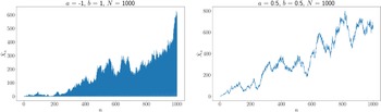
In Figure 7, we observe linear growth of the discrete-time process
 $\widetilde{X}_n$
, with oscillations to 0 when
 $a<0$
and
 $b=1$
(left panel) and without oscillations in the case
 $a+b=1$
. The situation seems to be different for
 $a\ge2$
and
 $b=-a^2/4$
. When
 $a>2$
we observe exponential growth (Figure 8 (left)), similar to the transient regime, while the case
 $a=2$
presents large excursions away from 0, but deciphering transient or recurrent behaviour is difficult. These simulations show that the study of these critical cases is an interesting research topic for the future.
Trajectories of
 $(\widetilde{X}_n)_{0\le n\le 1000}$
for critical parameters
 $(a,b)=(\!-\!1,1)$
on the left and
 $(a,b)=(0.5,0.5)$
on the right. We observe linear growth of the process as could be expected in critical cases.

Trajectories of
 $(\widetilde{X}_n)_{0\le n\le 1000}$
for critical parameters
 $(a,b)=(4,-4)$
on the left and
 $(a,b)=(2,-1)$
on the right.

5.2. Generalization of the model
As explained at the beginning of the article, the results obtained here should be seen as a starting point for the search for necessary and sufficient conditions for the stability of Hawkes processes with inhibition, in discrete or continuous time.
We believe that obtaining a similar classification in the cases
 $p>2$
or
 $p=\infty$
is a very difficult problem. It should be closely related to the study of the asymptotic behaviour of certain deterministic equations, such as the non-linear recurrence equation
 $x_n = (a_1x_{n-1}+\cdots+a_px_{n-p})_+$
. It seems that the algebraic structures underlying these equations are intricate and, to this date, unknown. Understanding these structures seems crucial for the study of the asymptotic behaviour of the solutions to these equations.
Appendix A. Linear recurrence equations
Let
 $\alpha \in \mathbb{R}$
,
 $p\in \mathbb{N}$
, and
 $a_1,\ldots,a_p \in \mathbb{R}$
. Consider the linear recurrence equation
 \begin{align*}x_n = a_1x_{n-1} + \cdots + a_px_{n-p} + \alpha,\qquad n\ge 1,\end{align*}
with given initial data
 $x_{0},\ldots,x_{-p+1}\in \mathbb{R}$
. Define the matrix
 \begin{align*}A = \left(\begin{array}{c@{\quad}c@{\quad}c@{\quad}c}a_1 & \cdots & a_{p-1} & a_p\\[5pt] 1 & & &\\[5pt] & \ddots & & \\[5pt] & & 1 &\end{array}\right),\end{align*}
where vanishing entries are meant to be zero. Then, setting
 \begin{align*}\bar x_n = \begin{pmatrix}x_n\\[5pt] \vdots\\[5pt] x_{n-p+1}\end{pmatrix}, \qquad \bar \alpha = \begin{pmatrix}\alpha\\[5pt] 0\\[5pt] \vdots \\[5pt] 0\end{pmatrix},\end{align*}
the sequence
 $(\bar x_n)_{n\ge 1}$
solves the system of linear recurrences
 $\bar x_n = A \bar x_{n-1} + \bar \alpha$
,
 $n\ge 1$
. Recall that the spectral radius
 $\rho(A)$
of the matrix A is defined by
 $\rho(A) = \max(|\theta_1|,\ldots,|\theta_p|)$
, where
 $\theta_1,\ldots,\theta_p\in \mathbb{C}$
are the complex eigenvalues of A, counted with algebraic multiplicity. Equivalently,
 $\theta_1,\ldots,\theta_p$
are the roots, counted with multiplicity, of the characteristic polynomial
 $P(z) = \det(zI - A) = z^p - a_1z^{p-1} - \cdots -a_p$
.
We recall the following classical fact.
Theorem 3. ([Reference Gallier and Quaintance9, Chapter 9, Theorem 9.1]) The following are equivalent:
-
(i)
$\bar x_n$
converges as
$n\to\infty$
for every initial data point
$x_0,\ldots,x_{-p+1}$
. -
(ii)
$\rho(A) < 1$
.


In the case
 $p=2$
, setting
 $a = a_1$
and
 $b=a_2$
, we have
 $\mathbb{P}(z) = z^2 - az-b$
. Its roots are
 \begin{align*}\theta_\pm = \frac a 2 \pm \sqrt{\frac {a^2} 4 + b}.\end{align*}
In particular,
 \begin{align*}\rho(A) =\begin{cases} \dfrac{|a|}2 + \sqrt{\dfrac{a^2}4 + b} & \textrm{if }\dfrac{a^2}4 + b \ge 0, \\[10pt] \sqrt{-b} & \textrm{if } \dfrac{a^2}4 + b < 0.\end{cases}\end{align*}
A quick calculation shows that
 $\rho(A) < 1$
if and only if
 $|a| + b < 1$
and
 $b > -1$
. This corresponds to the triangular dashed region of parameters in Figure 1 of Section 2.
Appendix B. Criteria for strong irreducibility
The Markov chain considered in this article is irreducible in the (weak) sense of [Reference Douc, Moulines, Priouret and Soulier5], but not necessarily strongly irreducible, i.e. irreducible in the classical sense. In this section, we study the decomposition of the state space into communicating classes. We recall the basic definitions. Let
 $x,y\in \mathbb{N}^2$
. We say that x leads to y, or, in symbols,
 $x \to y$
, if there exists
 $n\ge 0$
such that
 $\mathbb{P}(X_n = y\mid X_0 =x) > 0$
. We say that x communicates with y if
 $x\to y$
and
 $y\to x$
. This is an equivalence relation that partitions the state space
 $\mathbb{N}^2$
into classes called communicating classes.
Recall that a Markov chain is called strongly irreducible if all states are accessible or, equivalently, if
 $\mathbb{N}^2$
is a communicating class. A communicating class
 $C\subset \mathbb{N}^2$
is called closed if
 $x\in C$
and
 $y\in C^\textrm{c}$
do not exist such that
 $x\to y$
.
Proposition 2. The Markov chain
 $(X_n)$
is strongly irreducible on
 $\mathbb{N}^2$
if and only if
 $a \geq 0$
, or if
 $a > -\lambda$
and
 $a+b \geq 0$
.
The communicating class of (0,0) contains
 \begin{equation} \mathcal{S} = \{(0, 0)\} \cup \{(0, k), k\in\mathbb{N}^*\} \cup \{(k, 0), k\in\mathbb{N}^*\}, \end{equation}
and is actually equal to
 $\mathcal{S}$
if and only if
 $a\le -\lambda$
.
We will use the following result.
Lemma 4. Let
 $i,j,k,\ell \in \mathbb{N}$
. The transition matrix P of the Markov chain
 $(X_k)$
satisfies
 \begin{align*}P^2((i, j), (k, \ell)) = \frac{\textrm{e}^{-(s_{ij}+s_{\ell i})}s_{ij}^\ell s_{\ell i}^k}{\ell!\,k!},\end{align*}
and, for all
 $n \geq 3$
,
 \begin{equation} P^n((i, j), (k, \ell)) = \sum_{m_1,\dots,m_{n-2}\in\mathbb{N}}\frac{\exp\big\{{-}\sum_{q=1}^n s_{\sigma_{q+1}^n\sigma_{q+2}^n}\big\} \prod_{q=1}^n s_{\sigma_{q+1}^n \sigma_{q+2}^n}^{\sigma_{q}^n }}{m_1! \cdots m_{n-2}! \,k! \,\ell!}, \end{equation}
with
 $\sigma^n \;:\!=\; (\sigma^n_1, \sigma^n_2, \dots, \sigma^n_{n+2}) = (k, \ell, m_{n-2}, \dots, m_1, i, j)$
.
Proof of Proposition
2. As mentioned above,
 $(i, j) \to (0, i) \to (0, 0)$
for any
 $(i,j) \in \mathbb{N}^2$
since it only requires that two successive 0s are drawn from the Poisson random variable. Therefore, to prove strong irreducibility, it is sufficient to prove that
 $(0, 0) \leadsto (i, j)$
for all
 $(i, j)\in\mathbb{N}^2$
. We consider different cases, depending on the values of the parameters a and b.
 $a \geq 0$
: Since
 $\lambda >0$
and
 $s_{00}>0$
, (j, 0) is accessible from (0, 0) for all
 $j\in \mathbb{N}$
. Moreover, when
 $a \geq 0$
,
 $s_{j0} = (aj + \lambda)_+ > 0$
and then
 $( j, 0 ) \to ( i, j )$
, yielding the result.
 $-\lambda < a < 0$
and
 $a+b \geq 0$
: Let
 $k \in \mathbb{N}$
. Since
 $a+b \geq 0$
and
 $a+\lambda >0$
,
 \begin{align*}s_{k+1,k} = (a(k+1) + bk + \lambda)_+ = ((a+b)k + a + \lambda)_+ > 0.\end{align*}
Let
 $( i, j ) \in \mathbb{N}^2$
. Since
 $s_{k+1,k}>0$
for all k, we deduce that any
 $(\ell, k+1)$
is accessible from
 $(k+1,k)$
. Thus, in order to reach (i, j) from (0,0), we move from small steps to
 $(j,j-1)$
, and then reach (i, j):
 \begin{align*}( 0, 0 ) \to ( 1, 0 ) \to ( 2, 1 ) \to \dots \to ( j, j-1 ) \to ( i, j ),\end{align*}
which concludes the proof of this case.
 $a \leq -\lambda$
: We prove that the communicating class of (0,0) is given by (19). Let
 $k \in \mathbb{N}^*$
. Then, as previously, we have
 $( 0, 0 ) \to ( k, 0 )$
since
 $s_{00}>0$
; however, since
 $a\leq -\lambda$
,
 $s_{k0} = (ak+\lambda)_+ = 0$
, and the next step of the Markov chain will be (0, k). Depending on the value of the parameter b, the next step of the Markov chain will either be (0, 0) if
 $s_{0k}=0$
, or (k’, 0) with
 $k'\geq 0$
if
 $s_{0k}>0$
, and so on. This proves that the class cl(0,0) is closed and given by (19).
 $-\lambda < a < 0$
and
 $a+b < 0$
: In this case we can only prove that the Markov chain is not strongly irreducible on
 $\mathbb{N}^2$
, but we do not identify the communicating class of (0,0). There are three subcases to consider.
First,
 $b< 0$
. Since
 $a<0$
, we can choose
 $k_\star$
such that
 $ak_\star + \lambda \leq 0$
. We show that it is not possible to reach the state
 $( 1, k_\star )$
. Assuming the opposite leads to the existence of
 $\ell \in \mathbb{N}$
such that
 $(k_\star, \ell) \to (1, k_\star)$
, which implies that
 $s_{k_\star, \ell} > 0$
. If
 $b<0$
, we deduce that, necessarily,
 \begin{align*}ak_\star + b\ell + \lambda > 0 \Longrightarrow \ell < \dfrac{-ak_\star - \lambda}{b} \leq 0,\end{align*}
so
 $\ell < 0$
, which is contradictory. We then deduce that the Markov chain is reducible.
Second, if
 $b=0$
,
 $s_{k_\star, \ell} > 0$
would imply that
 $ak_\star + \lambda > 0$
, which contradicts the definition of
 $k_\star$
.
Third,
 $b>0$
. Since
 $a+b < 0$
, it is possible to choose
 $k_\star \in \mathbb{N}$
large enough that
 $(a+b)k_\star + \lambda \leq 0$
. In particular,
 $0 \geq ak_\star+bk_\star+\lambda \geq ak_\star+\lambda$
, so
 \begin{align*}\dfrac{-ak_\star - \lambda}{b} \geq k_\star \geq \dfrac{-\lambda}{a}.\end{align*}
Notice that
 $k_\star \geq 2$
since
 $k_\star \geq {-\lambda}/{a} > 1$
.
We show that it is not possible to reach
 $(1, k_\star)$
starting from (0, 0). Assuming the opposite leads us to the existence of
 $n \in \mathbb{N}$
such that
 $P^n((0, 0),(1, k_\star)) > 0$
. Using (20) in Lemma 4 implies that
 $m_1, \dots, m_{n-2} \in \mathbb{N}$
exist such that
 \begin{align*} \left\{ \begin{array}{ll} s_{k_\star,m_{n-2}} > 0, \\[5pt] s_{m_{n-2} m_{n-3}}^{k_\star} > 0, \\[5pt] \qquad \vdots \\[5pt] s_{m_2 m_1}^{m_3} > 0, \\[5pt] s_{m_1 0}^{m_2} > 0. \end{array} \right. \end{align*}
We thus have
 \begin{align*}ak_\star + bm_{n-2} + \lambda > 0 \Longrightarrow m_{n-2} > \dfrac{-ak_\star - \lambda}{b} \geq k_\star;\end{align*}
then, since
 $k_\star > 0$
, we necessarily have
 $s_{m_{n-2}m_{n-3}}>0$
. This yields
 \begin{align*} am_{n-2} + bm_{n-3} + \lambda > 0 \Longrightarrow m_{n-3} > \dfrac{-a m_{n-2} - \lambda}{b} \geq \dfrac{-ak_\star - \lambda}{b} \geq k_\star. \end{align*}
By immediate induction, we thus have, for all
 $i \in \{ 1, \dots,n-2 \}$
,
 $m_i \geq k_\star \geq {-\lambda}/{a}$
. Finally,
 $s_{m_1,0} > 0$
implies
 $a m_1 + \lambda > 0$
, which is contradictory. We conclude that there is no finite path between (0, 0) and
 $( 1, k_\star )$
, so the Markov chain
 $(X_k)_{k\ge0}$
is reducible on
 $\mathbb{N}^2$
.
Acknowledgements
We thank two anonymous reviewers for their valuable suggestions, which helped to improve the presentation of the paper.
Funding information
M.C. was supported by the Chair ‘Modélisation Mathématique et Biodiversité’ of Veolia Environnement-École Polytechnique-Muséum national d’Histoire naturelle-Fondation X and by ANR project HAPPY (ANR-23-CE40-0007) and DEEV (ANR-20-CE40-0011-01). P.M. acknowledges partial support from ANR grant ANR-20-CE92-0010-01 and from Institut Universitaire de France.
Competing interests
There were no competing interests to declare which arose during the preparation or publication process of this article.