





1. Introduction
Magnetic reconnection is thought to be the dynamical mechanism responsible for many explosive phenomena observed in laboratory, space and astrophysical plasmas (Yamada, Kulsrud & Ji Reference Yamada, Kulsrud and Ji2010; Pucci et al. Reference Pucci2020b ; Ji & Daughton Reference Ji and Daughton2022). Through magnetic topology reconfiguration, reconnection converts stored magnetic energy into plasma heating, particle acceleration and bulk flows. This mechanism is central to energy release events in magnetic confinement fusion devices (e.g. tokamak sawtooth crashes (Waelbroeck Reference Waelbroeck1989)), solar flares and coronal mass ejections in the solar corona (Shibata Reference Shibata1996), geomagnetic storms and substorms within planetary magnetospheres (Louarn et al. Reference Louarn, Andre, Jackman, Kasahara, Kronberg and Vogt2015; Burch & Phan Reference Burch and Phan2016) and high-energy phenomena in astrophysical environments such as accretion disks and relativistic jets (Romanova & Lovelace Reference Romanova and Lovelace1992; Khiali & de Gouveia Dal Pino Reference Khiali, de Gouveia Dal and Elisabete2016).
The tearing-mode instability, first analysed by Furth, Killeen & Rosenbluth (Reference Furth, Killeen and Rosenbluth1963), is a fundamental mechanism through which magnetic reconnection can develop within current sheets in the resistive magnetohydrodynamic (MHD) framework. Over the past several decades, the tearing mode has been investigated extensively under increasingly complex plasma conditions. Studies have explored its properties with equilibrium shear flows and/or viscosity (Chen & Morrison Reference Chen and Morrison1990; Ofman et al. Reference Ofman, Chen, Morrison and Steinolfson1991; Dahlburg, Boncinelli & Einaudi Reference Dahlburg, Boncinelli and Einaudi1997; Grasso et al. Reference Grasso, Hastie, Porcelli and Tebaldi2008; Tenerani et al. Reference Tenerani, Rappazzo, Velli and Pucci2015; Comisso & Grasso Reference Comisso and Grasso2016; Mallet et al. Reference Mallet, Eriksson, Swisdak and Juno2025), incorporated Hall and two-fluid effects (Terasawa Reference Terasawa1983; Pucci, Velli & Tenerani Reference Pucci, Velli and Tenerani2017; Shi et al. Reference Shi, Velli, Pucci, Tenerani and Innocenti2020) and extended to partially ionised plasmas (Paris Reference Paris1973; Zweibel et al. Reference Zweibel, Lawrence, Yoo, Ji, Yamada and Malyshkin2011; Pucci et al. Reference Pucci, Singh, Tenerani and Velli2020a ) and to collisionless or kinetic regimes (Porcelli Reference Porcelli1991; Daughton & Karimabadi Reference Daughton and Karimabadi2005; Del Sarto et al. Reference Del Sarto, Pucci, Tenerani and Velli2016).
However, in many natural and laboratory environments reconnection can occur in stratified plasmas in the presence of gravity, magnetic curvature, or other effective accelerations, sometimes leading to heavy-over-light plasma configurations embedded within current sheets. At Earth’s magnetopause, for example, rapid variations in solar wind dynamic pressure accelerate the boundary across the sharp density gradient separating the dense magnetosheath from the tenuous magnetosphere, producing an effective gravitational force that can drive Rayleigh–Taylor modes (Anderson, Binsack & Fairfield Reference Anderson, Binsack and Fairfield1968; Gratton, Farrugia & Cowley Reference Gratton, Farrugia and Cowley1996) and potentially affect reconnection during southward interplanetary magnetic field conditions. Similar conditions arise at the heliopause, where both acceleration of the heliospheric interface towards the interstellar medium and charge-exchange interactions between interstellar neutrals and heliosheath plasma can generate an effective gravity antiparallel to the density gradient, making the interface unstable to Rayleigh–Taylor modes (Borovikov et al. Reference Borovikov, Pogorelov, Zank and Kryukov2008; Avinash et al. Reference Avinash, Zank, Dasgupta and Bhadoria2014; Pogorelov et al. Reference Pogorelov, Heerikhuisen, Roytershteyn, Burlaga, Gurnett and Kurth2017; Opher et al. Reference Opher2021; Ruderman Reference Ruderman2024). In the laboratory, magnetic confinement devices such as tokamaks and stellarators are also susceptible to interchange-type instabilities (Kruskal & Schwarzschild Reference Kruskal and Schwarzschild1954) and other gravity-driven resistive instabilities that can develop in current sheets (Furth et al. Reference Furth, Killeen and Rosenbluth1963; Johnson, Greene & Coppi Reference Johnson, Greene and Coppi1963; Coppi Reference Coppi1964; Roberts & Taylor Reference Roberts and Taylor1965; Glasser, Greene & Johnson Reference Glasser, Greene and Johnson1975). These early works, however, relied on restrictive assumptions – such as constant
 $\psi$
, weak gravity, weak magnetic shear or asymptotic wavelength limits – thereby limiting their ability to capture how tearing modes are modified by gravity and how they transition to gravity-driven instabilities.
In this study, we investigate the effects of favourable and unfavourable stratification on the linear stage of reconnecting instabilities in a plane slab current sheet by including a gravitational acceleration acting normal to the current layer. Here, favourable and unfavourable stratifications refer to cases in which the density gradient is parallel or antiparallel, respectively, to the gravitational acceleration. Although configurations with a negative density gradient along the gravitational field direction (unfavourable stratification) can be ideally unstable to interchange or Rayleigh–Taylor modes, we restrict our attention to regimes in which stratification is sufficiently weak to satisfy the Suydam stability criterion (Gerwin Reference Gerwin1979; Paris et al. Reference Paris1982), a necessary condition for ideal stability in a sheared pinch configuration.
With uniform resistivity, it has been shown that a plane sheet pinch is unstable to two resistive instabilities under the constant-
 $\psi$
approximation (Furth et al. Reference Furth, Killeen and Rosenbluth1963): a long-wavelength tearing mode, dominant when gravity is negligible, with a growth rate scaling with the Lundquist number as
 $S^{-3/5}$
, and a short-wavelength gravity-driven mode (the G-mode) with a growth rate scaling as
 $S^{-1/3}$
. This gravity-driven resistive mode was further extended to stellarator-like geometry in weakly sheared magnetic configurations (Johnson et al. Reference Johnson, Greene and Coppi1963; Coppi Reference Coppi1964; Roberts & Taylor Reference Roberts and Taylor1965) and generalised to non-localised modes manifesting as twisted convective rolls (Roberts & Taylor Reference Roberts and Taylor1965). Recently, Hopper, Wood & Bushby (Reference Hopper, Wood and Bushby2024) investigated the effect of favourable stratification on the linear growth rate of the tearing mode in slab geometry using both analytical and numerical approaches. They found that increasing the stabilising density gradient suppresses the growth of tearing perturbations. Here, we follow their approach in solving the resistive-layer equations assuming a linear density profile, but extend their analysis to include unfavourable stratification, allowing for gravity-driven instabilities. We derive the general dispersion relation that describes the continuous transition from the tearing-dominated regimes to G-modes and examine how the growth rate depends on both the stratification strength (favourable and unfavourable) and the Lundquist number. In addition, we numerically investigate a more realistic equilibrium density profile with a smooth transition between two plasma regions to assess the sensitivity of the growth rate to the density profile.
The plan of the paper is as follows. We begin in § 2 by introducing the set of equations describing the tearing mode and derive layer equations in §§ 3.1 and 3.2. In § 3.3, we show the dispersion relation obtained by applying the asymptotic matching technique. In § 4 we compare analytical and numerical results and investigate the effects of stratification on the growth rate of the tearing mode. Conclusions of this study are given in § 5.
2. Model equations
We start from the resistive MHD equation set that neglects plasma compressibility and incorporates uniform plasma resistivity:
 \begin{align} \frac {\partial \rho }{\partial t} +\boldsymbol{\nabla }\boldsymbol{\cdot }(\rho \boldsymbol{V}) = 0 , \end{align}
 \begin{align} \rho \frac {\partial \boldsymbol{V}}{\partial t} + \rho \boldsymbol{V}\boldsymbol{\cdot}\boldsymbol{\nabla }\boldsymbol{V} = - \boldsymbol{\nabla }P + \boldsymbol{J}\times \boldsymbol{B} + \rho \boldsymbol{g} , \end{align}
 \begin{align} \frac {\partial \boldsymbol{B}}{\partial t} =\boldsymbol{\nabla }\times (\boldsymbol{V}\times \boldsymbol{B})+ \frac {\eta }{\mu _{o}} {\nabla} ^{2}\boldsymbol{B}, \end{align}
 \begin{align} \boldsymbol{\nabla }\boldsymbol{\cdot} \boldsymbol{V} = 0, \end{align}
where
 $\rho$
,
 $\boldsymbol{V}$
,
 $P$
and
 $\boldsymbol{B}$
are the density, velocity, scalar pressure and magnetic field, respectively,
 $\boldsymbol{J} = \boldsymbol{\nabla }\times \boldsymbol{B}/\mu _{0}$
is the current density,
 $\boldsymbol{g}$
is the gravitational acceleration acting in the negative
 $x$
direction and
 $\eta$
is the resistivity.
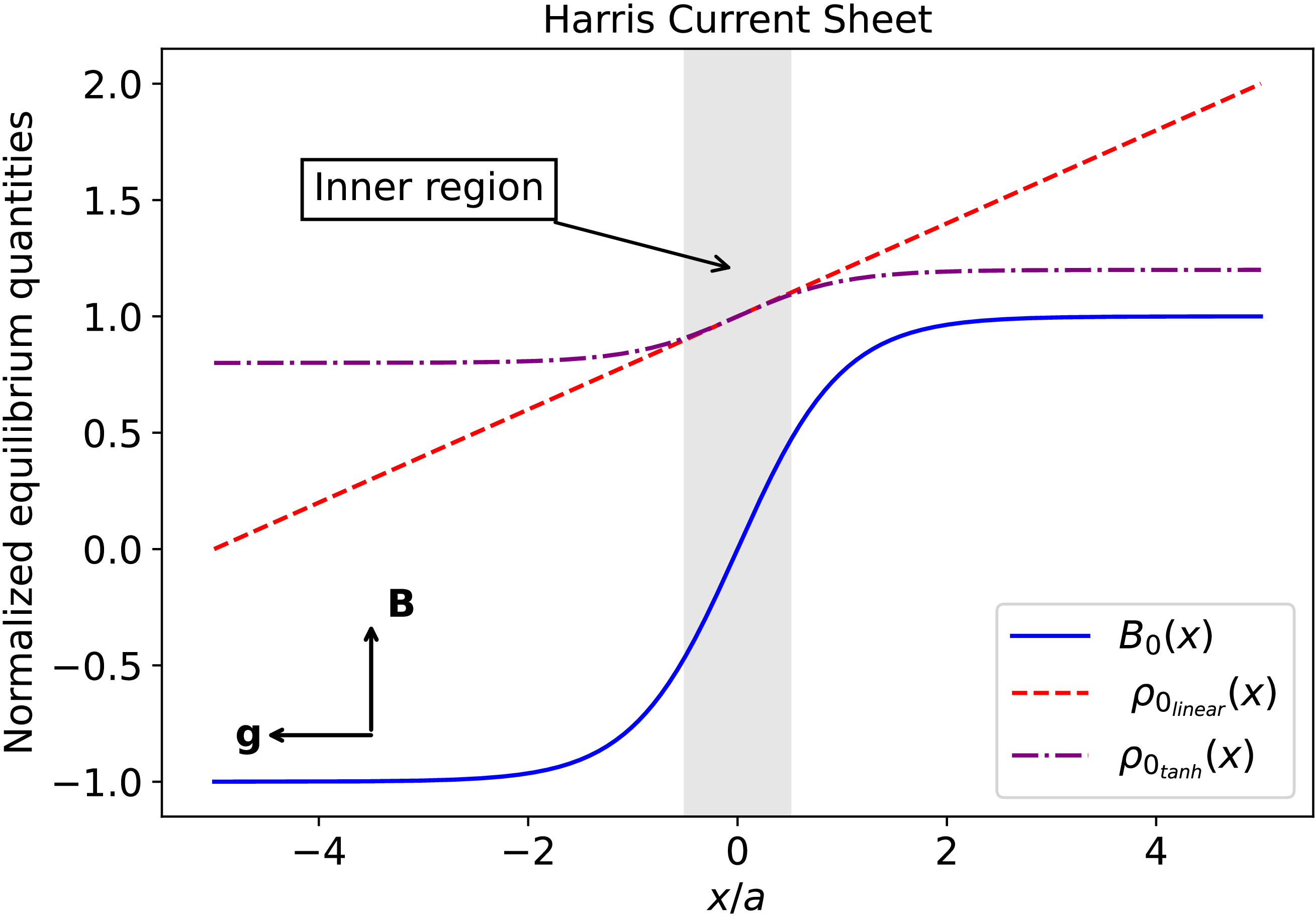
Our equilibrium, illustrated schematically in figure 1, is characterised by an inhomogeneous plasma embedded in a Harris-type current sheet (Harris Reference Harris1962), defined by the following in-plane magnetic field and plasma density:
 \begin{align} \boldsymbol{B}_{0} = B_{0} \tanh \left (\frac {x}{a}\right ) \boldsymbol{\hat {y}}, \end{align}
 \begin{align} \rho _{0}(x) = \bar {\rho }_{0}\left (1+\epsilon \frac {x}{a}\right ), \end{align}
where
 $a$
is the current sheet half-thickness and
 $\bar {\rho }_{0}$
is a constant. We assume a weak density inhomogeneity (
 $\epsilon \ll 1$
) in order to apply the Boussinesq approximation. Our choice of the linear density profile enables an analytic solution to the outer equation. This profile can be regarded as an approximation near the resonant surface of the more physically realistic tanh density profile introduced later (see (4.2)), since
 $\tanh (x/a)\approx x/a$
for
 $|x/a|\ll 1$
. Consequently, the behaviour of the outer solution should be interpreted as a consequence of this modelling choice. The background flow is set to zero everywhere (
 $\boldsymbol{V}_{0} ={\boldsymbol 0 }$
) and the equilibrium is achieved with a background pressure
 $P_{0}(x)$
such that
 \begin{align} P_0(x) + \frac {B_{0}^{2}}{2\mu _{o}}+\bar {\rho }_{0}\left (x+\epsilon \frac {x^2}{2a}\right )g = P_0(0). \end{align}
Schematic of the equilibrium configuration within the Harris-type current sheet in the presence of an effective gravitational field, highlighting the equilibrium magnetic field and the two density profiles considered in this work: the linear profile (2.6) and the hyperbolic tangent profile (4.2).

The configuration described above satisfies the equilibrium conditions of ideal MHD. However, when finite resistivity is included, the magnetic field diffuses on the resistive diffusion time scale
 $\tau _R=\mu _{o}a^2/\eta$
. In this work, we focus on weakly collisional plasmas, where resistivity is assumed to be sufficiently small such that the diffusion rate is negligible compared with the instability growth rate, allowing us to neglect resistive diffusion in the analysis. An exception arises in the favourable stratification asymptotic regime, where we will show that
 $\gamma \tau _A \sim S^{-1}$
(§ 4.3). In this limit, the instability growth time scale becomes comparable to the resistive diffusion time scale of the equilibrium current sheet, and the assumption of a fixed equilibrium is therefore no longer self-consistent. As discussed in § 4.3, the
 $S^{-1}$
scaling should thus be regarded as a formal asymptotic result obtained under the assumption of a frozen equilibrium; unless the current sheet is externally maintained, its resistive evolution must be taken into account.
In the context of a stratified atmosphere it is common to adopt entropy, rather than density, as the dynamically advected thermodynamic variable within the Boussinesq approximation. Our work, however, is intended to describe a different physical regime: an incompressible current sheet embedded between plasma regions of different densities in an effective gravitational field, rather than a self-consistent stratified atmosphere. The motivation is to model environments such as the magnetopause and heliopause, which are characterised by a density gradient between adjacent plasma regions. In such systems, the relevant buoyancy effect arises directly from the density gradient across the interface, analogous to Rayleigh–Taylor/interchange instability, rather than from an entropy gradient. Accordingly, we adopt an incompressible description in which the equilibrium density profile is prescribed and weakly varying, while compressibility effects are neglected. Density variations are retained only in the gravitational (buoyancy) term and neglected elsewhere to leading order, consistent with Boussinesq ordering. Consequently, the stratification parameter
 $A$
(introduced later in (2.13)) measures the stabilising or destabilising effect of an imposed density variation in the presence of gravity, rather than the Brunt–Väisälä response of a stratified atmosphere.
To linearise the system of equations (2.1)–(2.4), we first introduce the two scalar stream (
 $\phi$
) and flux (
 $\psi$
) functions such that
 \begin{align} \boldsymbol{V} = \boldsymbol{\nabla }\phi \times \boldsymbol{\hat {z}}, \end{align}
 \begin{align} \boldsymbol{B} = \boldsymbol{\nabla }\psi \times \boldsymbol{\hat {z}}. \end{align}
We consider small fluctuations of the form
 $f(x/a) \,\mathrm{exp} (iky+\gamma t)$
, where
 $\gamma$
and
 $k$
denote the growth rate and wave vector of a given mode, respectively. Linearising the MHD equations around the prescribed equilibrium and introducing these perturbations, we obtain two coupled equations for the normalised flow and magnetic flux perturbations
 $\hat {\phi }$
and
 $\hat {\psi }$
:
 \begin{align} \hat {\gamma } S (\hat {\psi } -F \hat {\phi }) = (\hat {\psi }^{\prime \prime }-\hat {k}^{2} \hat {\psi }), \end{align}
 \begin{align} \hat {\gamma }^{2} ( \hat {\phi }^{\prime \prime }- \hat {k}^{2} \hat {\phi }) =- \hat {k}^{2} F \left (\hat {\psi }^{\prime \prime } -\hat { k}^{2} \hat {\psi } - \frac {F^{\prime \prime }}{F} \hat {\psi }\right ) - \frac {a \mu _{0}}{B_{0}^{2}} g \hat {k}^{2}\hat {\phi } \frac {{\rm d}\rho _{0}}{{\rm d}\hat {x}}- \frac {\hat {\gamma }^{2}}{{\bar \rho _{0}}}\hat {\phi }^{\prime }\frac {{\rm d}\rho _{0}}{{\rm d}\hat {x}}. \end{align}
In the equations above, a prime denotes differentiation with respect to the normalised variable
 $\hat {x}=x/a$
,
 $\hat {k}=ka$
and
 $\hat {\gamma }=\gamma \tau _a$
, where
 $\tau _{a}=a/V_{A}$
is the Alfvèn crossing time with
 $V_{A}=B_0/\sqrt {\mu _0\bar {\rho }_0}$
being the Alfvèn speed and
 $\bar {\rho }_{0}$
is the density at the neutral line (
 $x=0$
). Flow and flux functions are normalised to
 $\psi = - a B_{0} \hat {\psi }$
and
 $\phi = i({\gamma a}/{k})\hat {\phi }$
. Here,
 $F=\tanh {(\hat {x})}$
and
 $S = \mu _{0}aV_{A}/\eta$
is the Lundquist number.
Equation (2.11) has been obtained by taking the
 $z$
component of the curl of (2.2) and then by approximating
 $\rho _0^{-1}\simeq 1/\bar \rho _0$
to zeroth order in
 $\epsilon$
. We consider the asymptotic limit
 $\epsilon \rightarrow 0$
while holding the stratification parameter, defined in (2.13),
 $A\sim \epsilon ({ga}/{V^2_A})$
finite and small,
 $A\ll 1$
, which implies
 $({ag}/{V^2_A})\sim \epsilon ^{-1}$
. Under this ordering, the last term in (2.11), which is directly proportional to parameter
 $\epsilon$
, vanishes as
 $\epsilon \rightarrow 0$
. Whereas, the buoyancy term remains finite through the combination
 $A=\epsilon ({ga}/{V^2_A})$
. Therefore, the last term can be consistently neglected while a weak but finite buoyancy contribution is retained. Importantly, its omission allows us to solve the eigenvalue problem by imposing specific parity conditions on the eigenfunctions. The resulting equation for the stream function is
 \begin{align} \hat {\gamma }^{2} ( \hat {\phi }^{\prime \prime }- \hat {k}^{2} \hat {\phi }) =- \hat {k}^{2} F \left (\hat {\psi }^{\prime \prime } -\hat { k}^{2} \hat {\psi } - \frac {F^{\prime \prime }}{F} \hat {\psi }\right ) - A \hat {k}^{2}\hat {\phi }, \end{align}
where
 \begin{align} A = \frac {a \mu _{0}}{B_{0}^{2}} g \frac {{\rm d}\rho _{0}}{{\rm d}\hat {x}}=\epsilon \frac {a g}{V_{a}^2}, \end{align}
represents the stratification parameter and characterises the strength of stratification, which can be either unfavourable or favourable. According to (2.13), the type of stratification can be controlled through the sign of
 $\epsilon$
in (2.6):
 $\epsilon \lt 0$
corresponds to favourable stratification, whereas
 $\epsilon \gt 0$
indicates unfavourable stratification. As we mentioned earlier, unfavourable stratification corresponds to the case where the density gradient is antiparallel to the effective gravitational field, resulting in positive values of
 $A$
. On the other hand, favourable stratification refers to the situation where the density gradient and effective gravitational field are aligned, yielding a negative value of
 $A$
.
The eigenfunctions of (2.10) and (2.12) exhibit well-defined parity: the ideal RT mode has the magnetic flux function
 $\hat {\psi }$
odd and the velocity stream function
 $\hat {\phi }$
even, whereas the tearing mode has
 $\hat {\psi }$
even and
 $\hat {\phi }$
odd. In what follows, we seek solutions to these equations that satisfy the tearing-mode parity.
3. Boundary-layer approach
In this section, we derive the analytic form of the dispersion relation by asymptotically matching the outer- and inner-region solutions. We begin with the outer-layer equations and their solution followed by the solution of the inner layer, and finally we derive the dispersion relation.
3.1. Outer region
For
 $S\gg 1$
, the dynamics is well described by ideal MHD far from the boundary layer. In such ideal outer region, one can therefore neglect plasma resistivity in (2.10) as well as plasma inertia in (2.12) and obtain the following ideal equations:
 \begin{align} \hat {\psi }= F\hat {\phi }, \end{align}
 \begin{align} F\left (\hat {\psi }^{\prime \prime } -\hat { k}^{2} \hat {\psi } -\frac {F^{\prime \prime }}{F} \hat {\psi }\right ) + A \hat {\phi } = 0. \end{align}
Upon inserting equation (3.1) into (3.2) one can eliminate the flux function and obtain a second-order equation for
 $\hat \phi$
:
 \begin{align} F^{2}\hat {\phi }^{\prime \prime }+ 2 F F^{\prime } \hat {\phi }^{\prime } +(A-\hat {k}^{2} F^{2})\,\hat {\phi } =0. \end{align}
Note that this equation, in the limit
 $|\hat {x}| \rightarrow \infty$
, admits two distinct types of solutions depending on the sign of the coefficient (
 $A - \hat {k}^{2}$
). If
 $A - \hat {k}^{2} \lt 0$
, the solution exhibits an exponentially decaying behaviour. In contrast, if
 $A - \hat {k}^{2}\gt 0$
, the solution is instead oscillatory. Such a non-localised character of the outer solution is an artefact of the linear density profile chosen for analytic tractability, and can be mitigated by imposing a smooth profile of
 $\rho _{0}(x)$
that asymptotes to constant values for
 $|\hat x|\rightarrow \infty$
. We will consider the latter density profile when discussing our results in § 4.
To perform the asymptotic matching between the outer and inner solutions, we first determine the behaviour of the outer solution near the resistive layer. To achieve this, we apply the Frobenius expansion technique to obtain a power-series solution to (3.3) for
 $|\hat {x}|\rightarrow 0$
, where the leading exponent is determined by the corresponding indicial equation. The general solution is then expressed as a linear combination of the leading terms of two linearly independent solutions corresponding to the roots of the indicial equation, and can be written as
 \begin{align} \hat {\phi }(\hat {x}) = c_{1}\hat {x}^{-l-({1}/{2})} +c_{2} \hat {x}^{l-({1}/{2})}, \end{align}
where
 $l = \sqrt {( {1}/{4})-A}$
. To ensure a power-law behaviour near the resistive layer, the condition
 $A\lt 1/4$
must be satisfied, a requirement that corresponds to the Suydam stability condition for our geometry (Paris et al. Reference Paris1982). The constants
 $c_{1}$
and
 $c_{2}$
are determined by comparing (3.4) with the complete solution of (3.3) in the limit
 $|\hat {x}|\rightarrow 0$
(see Appendix A). For
 $\hat {k}^{2}\gt A$
this leads to
 \begin{align} \hat {\phi }(\hat {x})= \left [a_{0} |\hat {x}|^{-l-({1}/{2})}+b_{0} |\hat {x}|^{l-({1}/{2})}\right ]\,\mathrm{sgn}(\hat {x}), \end{align}
where the coefficients are
 \begin{align} a_{0} = \frac {\varGamma (1+\nu )\varGamma (l)}{\varGamma \left (\frac {\nu }{2}+\frac {l}{2}+\frac {5}{4}\right )\varGamma \left (\frac {\nu }{2}+\frac {l}{2}-\frac {1}{4}\right )}, \end{align}
 \begin{align} b_{0} = \frac {\varGamma (1+\nu )\varGamma (-l)}{\varGamma \left (\frac {\nu }{2}-\frac {l}{2}+\frac {5}{4}\right )\varGamma \left (\frac {\nu }{2}-\frac {l}{2}-\frac {1}{4}\right )}. \end{align}
For the case
 $A\gt \hat {k}^{2}$
, the solution takes instead the form
 \begin{align} \hat {\phi }(\hat {x})=\left [a_{0mod} |\hat {x}|^{-l-({1}/{2})}+b_{0mod} |\hat {x}|^{l-({1}/{2})}\right ]\,\mathrm{sgn}(\hat {x}), \end{align}
where the modified coefficients
 $a_{0mod}$
and
 $b_{0mod}$
are
 \begin{align} a_{0 mod} = \frac {\varGamma (1+\nu )\varGamma (l)}{\varGamma \left (\frac {\nu }{2}+\frac {l}{2}+\frac {5}{4}\right )\varGamma \left (\frac {\nu }{2}+\frac {l}{2}-\frac {1}{4}\right )}+\frac {\varGamma (1-\nu )\varGamma (l)}{\varGamma \left (-\frac {\nu }{2}+\frac {l}{2}+\frac {5}{4}\right )\varGamma \left (-\frac {\nu }{2}+\frac {l}{2}-\frac {1}{4}\right )}, \end{align}
 \begin{align} b_{0mod} = \frac {\varGamma (1+\nu )\varGamma (-l)}{\varGamma \left (\frac {\nu }{2}-\frac {l}{2}+\frac {5}{4}\right )\varGamma \left (\frac {\nu }{2}-\frac {l}{2}-\frac {1}{4}\right )}+\frac {\varGamma (1-\nu )\varGamma (-l)}{\varGamma \left (-\frac {\nu }{2}-\frac {l}{2}+\frac {5}{4}\right )\varGamma \left (-\frac {\nu }{2}-\frac {l}{2}-\frac {1}{4}\right )}. \end{align}
In these coefficients
 $\nu =\sqrt {\hat {k}^2-A}$
. A detailed derivation of (3.5) and (3.8) is provided in Appendix A.
3.2. Inner region
In the inner layer, where perturbed magnetic and velocity fields exhibit sharp gradients and where reconnection occurs, resistive effects must be included. Due to these large gradients, we can assume that
 $\partial ^2/\partial \hat {x}^{2} \gg \hat {k}^{2}$
. In this way, the inner-region equations become
 \begin{align} \hat {\gamma } S (\hat {\psi } -\hat {x} \hat {\phi }) = \hat {\psi }^{\prime \prime }, \end{align}
 \begin{align} \hat {\gamma }^{2} \hat {\phi }^{\prime \prime } =- \hat {k}^{2} \hat {x} \hat {\psi }^{\prime \prime } - A\hat {k}^{2}\hat {\phi }. \end{align}
This set of equations is analytically solvable in Fourier space as the transformation with respect to the variable
 $\hat x$
reduces the original fourth-order ordinary differential equation system to a system of second-order differential equations in the variable
 $\hat {\theta }$
. To achieve asymptotic matching with the outer-region solution, the inner solution must be determined in the limit
 $\hat x\rightarrow \infty$
in configuration space, or
 $\hat \theta \rightarrow 0$
in Fourier space. In this limit, the Fourier-transformed stream function
 $\tilde {\phi }(\hat {\theta })$
is
 \begin{align} \tilde {\phi }(\hat {\theta })=\big[\tilde {a}_{0}|\hat {\theta }|^{l-({1}/{2})}+\tilde {b}_{0}|\hat {\theta }|^{-l-({1}/{2})}\big]\,\mathrm{sgn}(\hat {\theta }), \end{align}
where the coefficients
 $\tilde {a}_{0}$
and
 $\tilde {b}_{0}$
are given by the following forms:
 \begin{align} \tilde {a}_{0}=\left ({\frac {\sqrt {\hat {\gamma }/S}}{\hat {k}}}\right )^{ ({l}/{2})-( {1}/{4})}\frac {2\omega }{(\omega -l+\frac {1}{2})}\frac {\varGamma (-l)}{\varGamma \left (\left({(\omega -l)^{2}-\frac {1}{4}}\right)/{4\omega }\right )}, \end{align}
 \begin{align} \tilde {b}_{0}=\left ({\frac {\sqrt {\hat {\gamma }/S}}{\hat {k}}}\right )^{- ({l}/{2})- ({1}/{4})}\frac {2\omega }{(\omega +l+\frac {1}{2})}\frac {\varGamma (l)}{\varGamma \left (\left({(l+\omega )^{2}-\frac {1}{4}}\right)/{4\omega }\right )}, \end{align}
with
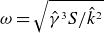 $\omega = \sqrt {{\hat {\gamma }^{3}S}/{\hat {k}^2}}$
. Appendix B contains the full derivation of (3.13).
3.3. Dispersion relation
To obtain the dispersion relation, we asymptotically match the outer and inner solutions in configuration space by using the asymptotic expressions provided in the previous sections. Thus, we first perform an inverse Fourier transform of the inner solution (3.13) into
 $\hat {x}$
space:
 \begin{align} \hat {\phi }(\hat {x})=\left [\bar {a}_{0}|\hat {x}|^{-l- ({1}/{2})}+\bar {b}_{0}|\hat {x}|^{l-({1}/{2})}\right ]\,\mathrm{sgn}(\hat {x}), \end{align}
where the coefficients
 $\bar {a}_{0}$
and
 $\bar {b}_{0}$
are related to the coefficients
 $\tilde {a}_{0}$
and
 $\tilde {b}_{0}$
, given by (3.14)–(3.15), as follows:
 \begin{align} \bar {a}_{0} = \frac {2}{i \pi }\left ({\frac {\sqrt {\hat {\gamma }/S}}{\hat {k}}}\right )^{ ({l}/{2})- ({1}/{4})}\frac {\omega \cos \left (\frac {\pi }{2}\left (\frac {1}{2}-l\right )\right ) }{\left (\omega -l+\frac {1}{2}\right )}\frac {\varGamma (\frac {1}{2}+l)\varGamma (-l)}{\varGamma \left (\left({(\omega -l)^{2}-\frac {1}{4}}\right)/{4\omega }\right )}, \end{align}
 \begin{align} \bar {b}_{0} = \frac {2}{i \pi }\left ({\frac {\sqrt {\hat {\gamma }/S}}{\hat {k}}}\right )^{-({l}/{2})- ({1}/{4})}\frac {\omega \cos \left (\frac {\pi }{2}\left (\frac {1}{2}+l\right )\right )}{\left (\omega +l+\frac {1}{2}\right )}\frac {\varGamma (\frac {1}{2}-l)\varGamma (l)}{\varGamma \left (\left({(\omega +l)^{2}-\frac {1}{4}}\right)/{4\omega }\right )}. \end{align}
Next, we match the coefficients of the two leading-order terms in (3.5) and (3.16) when
 $A-\hat {k}^2\lt 0$
, yielding the following dispersion relation:
 \begin{align} &\left ({\frac {\sqrt {\hat {\gamma }/S}}{\hat {k}}}\right )^{l}\frac {\left(\omega +l+\frac {1}{2}\right)}{\left(\omega -l+\frac {1}{2}\right)}\frac {\varGamma (-l)}{\varGamma (l)}\frac {\varGamma \left (\left({(\omega +l)^{2}-\frac {1}{4}}\right)/{4\omega }\right )}{\varGamma \left (\left({(\omega -l)^{2}-\frac {1}{4}}\right)/{4\omega }\right )}\nonumber\\[4pt] & \quad =\frac {\cos \left (\frac {\pi }{2}\left(\frac {1}{2}+l\right)\right )\varGamma \!\left(\frac {1}{2}-l\right)}{\cos \left (\frac {\pi }{2}\left(\frac {1}{2}-l\right)\right )\varGamma (\frac {1}{2}+l)}\frac {\varGamma (l)}{\varGamma (-l)}\frac {\varGamma \!\left(\frac {\nu }{2}-\frac {l}{2}+\frac {5}{4}\right)\varGamma \!\left(\frac {\nu }{2}-\frac {l}{2}-\frac {1}{4}\right)}{\varGamma \!\left(\frac {\nu }{2}+\frac {l}{2}+\frac {5}{4}\right)\varGamma \!\left(\frac {\nu }{2}+\frac {l}{2}-\frac {1}{4}\right)}. \end{align}
When
 $A -\hat {k}^2\gt 0$
the dispersion relation must be derived by matching the coefficients of the two leading-order terms in (3.8) and (3.16):
 \begin{align} &\left ({\frac {\sqrt {\hat {\gamma }/S}}{\hat {k}}}\right )^{l}\frac {\left(\omega +l+\frac {1}{2}\right)}{\left(\omega -l+\frac {1}{2}\right)}\frac {\varGamma (-l)}{\varGamma (l)}\frac {\varGamma \left (\left({(\omega +l)^{2}-\frac {1}{4}}\right)/{4\omega }\right )}{\varGamma \left (\left({(\omega -l)^{2}-\frac {1}{4}}\right)/{4\omega }\right )}\nonumber\\[3pt] & \quad =\frac {\cos \left (\frac {\pi }{2}\left(\frac {1}{2}+l\right)\right )\varGamma \!\left(\frac {1}{2}-l\right)}{\cos \left (\frac {\pi }{2}\left(\frac {1}{2}-l\right)\right )\varGamma \!\left(\frac {1}{2}+l\right)}\frac {\varGamma (l)}{\varGamma (-l)}\frac {\varGamma \!\left(\frac {\nu }{2}-\frac {l}{2}+\frac {5}{4}\right)\varGamma \!\left(\frac {\nu }{2}-\frac {l}{2}-\frac {1}{4}\right)}{\varGamma \!\left(\frac {\nu }{2}+\frac {l}{2}+\frac {5}{4}\right)\varGamma \!\left(\frac {\nu }{2}+\frac {l}{2}-\frac {1}{4}\right)} \nonumber\\[3pt] & \qquad \times \Bigg [{\left (1+\frac {\varGamma (1-\nu )\varGamma \!\left(\frac {\nu }{2}+\frac {l}{2}+\frac {5}{4}\right)\varGamma \!\left(\frac {\nu }{2}+\frac {l}{2}-\frac {1}{4}\right)}{\varGamma (1+\nu )\varGamma \!\left(-\frac {\nu }{2}+\frac {l}{2}+\frac {5}{4}\right)\varGamma \!\left(-\frac {\nu }{2}+\frac {l}{2}-\frac {1}{4}\right)}\right )}\Big /\nonumber\\[3pt] & \qquad {\left (1+\frac {\varGamma (1-\nu )\varGamma \!\left(\frac {\nu }{2}-\frac {l}{2}+\frac {5}{4}\right)\varGamma \!\left(\frac {\nu }{2}-\frac {l}{2}-\frac {1}{4}\right)}{\varGamma (1+\nu )\varGamma \!\left(-\frac {\nu }{2}-\frac {l}{2}+\frac {5}{4}\right)\varGamma \!\left(-\frac {\nu }{2}-\frac {l}{2}-\frac {1}{4}\right)}\right )}\Bigg ]. \end{align}
In the limit of no stratification (i.e.
 $A = 0$
), (3.19) reduces to the well-known dispersion relation of the standard tearing-mode instability (Fitzpatrick Reference Fitzpatrick2022) while the spectral range of validity of (3.20) narrows to zero.
4. Results
In this section, we compare the analytical results with the numerical solutions of (2.10) and (2.12) for both
 $A\gt 0$
and
 $A\lt 0$
to determine the effect of stratification on equilibrium stability. The numerical integration of (2.10) and (2.12) was performed using an adaptive finite-difference scheme based on Newton iteration which was designed by Lentini and Pereyra to solve boundary-value problems for systems of ordinary differential equations (Lentini & Pereyra Reference Lentini and Pereyra1974). This method was applied to compute the eigenvalues and eigenfunctions for two cases: the linear density profile (2.6) and a more realistic profile described by a hyperbolic tangent (4.2). For the analytical dispersion relations given in (3.19)–(3.20), we employed a Newton-type root-finding method, which iteratively finds zeros of a function starting from an initial guess and converges to the nearest root. Our results are summarised in figures 2–9.
4.1. Effect of linear stratification (linear profile)
According to the definition of the stratification parameter given in (2.13), for the linear density profile
 $A$
can be expressed as
 \begin{align} A = \frac {a\,g}{V_{A}^{2}}\,\epsilon . \end{align}
The analytical (solid lines) and numerical (dashed lines) dispersion relation for different favourable stratification values (
 $A\leqslant 0$
) for
 $S=10^6$
.

For stable stratification (
 $A\lt 0$
), figure 2 shows that as
 $|A|$
increases, the growth rate decreases, the range of unstable modes narrows and the fastest-growing mode shifts towards smaller wavelengths. These results are consistent with those of Hopper et al. (Reference Hopper, Wood and Bushby2024) and show excellent agreement between the analytic dispersion relation (solid lines) and the numerical solution to the eigenvalue problem (dashed lines).
The analytical (solid lines) and numerical (dashed lines) dispersion relation for different unfavourable stratification values (
 $A\geqslant 0$
) for
 $S=10^5$
.

Conversely, figure 3 shows that for unfavourable stratification (
 $A \gt 0$
) the tearing-mode growth rate increases with
 $A$
, and unstable modes extend to values
 $\hat {k} \gt 1$
. Note that in this figure the solid lines illustrate the dispersion relations (3.19) and (3.20), each within their valid regimes, namely
 $\hat {k}^{2} \gt A$
and
 $ \hat {k}^2 \lt A$
, respectively. The transition from oscillatory to exponentially localised solutions of the outer equation (3.3) occurs at
 $\hat {k}^{2} = A$
, producing peaks in the analytical results that are absent in the numerical solutions. This discrepancy arises from the finite domain used in numerical integration, which introduces a mismatch for
 $\hat k^{2} \lesssim A$
that is reduced by increasing the length of the integration domain. As discussed in § 3.1, this is an unphysical behaviour that can be mitigated by adopting a density profile that asymptotes to constant values far from the inner layer, ensuring spatial localisation of the eigenfunction. This case will be discussed next. Despite this discrepancy, excellent agreement between numerical and analytical solution is found for
 $\hat k^2\gt A$
. In this regime, stratification with
 $A \gt 0$
significantly increases the growth rate. Furthermore, unfavourable stratification couples the tearing mode with the gravity-driven G-mode thereby eliminating the marginally stable mode. In figures 2 and 3, the unstratified case is recovered for
 $A = 0$
(red colour), where the marginally stable mode asymptotically approaches
 $\hat {k} \rightarrow 1$
.
4.2. Effect of stratification with smooth transition (tanh profile)
A more realistic equilibrium density profile, instead of the form presented in (2.6), can be expressed as
 \begin{align} \rho _{0}(x) = \bar {\rho }_{0}\left (1+\epsilon \tanh \left ( \frac {x}{a}\right )\right ), \end{align}
which recovers the linear density profile for
 $|x|/a\ll 1$
but introduces a finite and smooth transition region between two well-defined plasma sectors. In this case, the equilibrium state must satisfy
 \begin{align} P_0(x)+\frac {B_{0}^{2}}{2\mu _{o}}+\bar {\rho }_{0}\left (x+\epsilon \,a\ln \left (\cosh {\left (\frac {x}{a}\right )}\right )\right )g = P_0(0), \end{align}
while the stratification parameter
 $A$
becomes
 \begin{align} A = \frac {a\,g}{V_{A}^{2}}\,\epsilon \,\mathrm{sech}^{2}{\left (\frac {x}{a}\right )}. \end{align}
Note that the parameter
 $A$
shown in the plots corresponds to evaluating this function at
 $x=0$
, which gives exactly the stratification
 $A$
of the linear profile (4.1).
Dispersion relation obtained by solving the eigenvalue problem numerically for the hyperbolic tangent density profile given in (4.2) for
 $A\leqslant 0$
and
 $S=10^6$
(left-hand panel) and
 $A\geqslant 0$
and
 $S=10^5$
(right-hand panel).

As shown in figure 4, the presence of both favourable and unfavourable stratification modifies the growth rate for the
 $\tanh$
profile mostly at large wave vectors,
 $\hat {k}\gtrsim \hat {k}_{m}$
, where
 $\hat {k}_m$
is the wave vector of the fastest-growing mode for
 $\hat {k}\lt 1$
, particularly those pertaining to the constant-
 $\psi$
regime (
 $\hat {k}\lesssim 1$
). On the contrary, the growth rate in the non-constant-
 $\psi$
regime remains essentially unaffected. More specifically, the left-hand panel shows that the growth rate decreases and the range of unstable modes narrows with increasing stratification strength
 $|A|$
. On the other hand, the right-hand panel illustrates that the system becomes less stable and the growth rate increases as the parameter
 $A$
increases leading to a modified tearing regime. Again, a marginal stable mode does not exist for
 $A\gt 0$
, indicating a smooth transition between tearing (
 $\hat {k}\lt 1$
) and the G-mode at values
 $\hat {k}\gt 1$
.
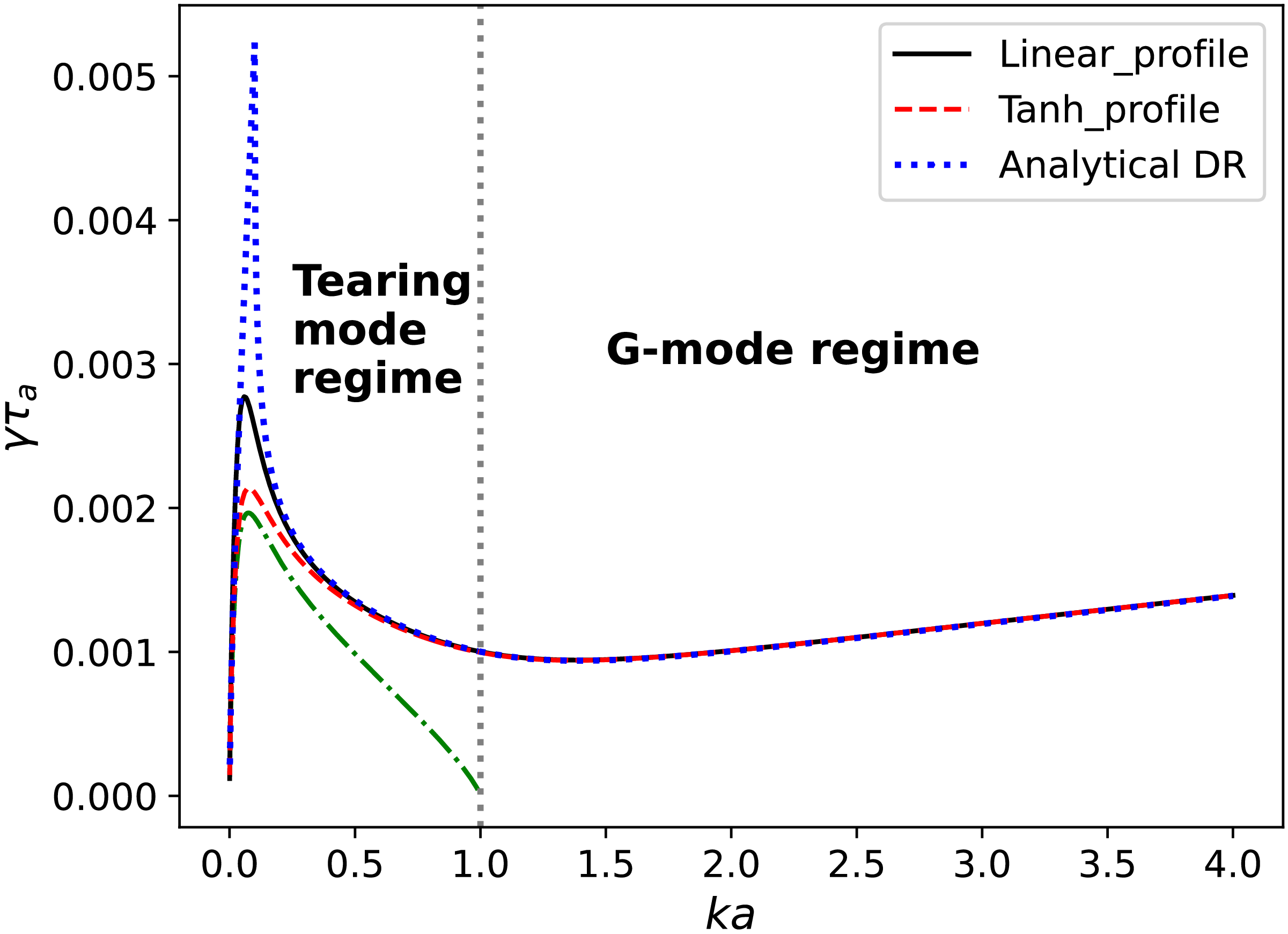
The analytical (dotted line) and numerical (solid and dashed lines) dispersion relation highlighting the effect of stratification on the tearing mode and the region of instability of G-modes for the density profiles given in (2.6) and (4.2) for
 $S= 10^{5}$
and
 $A = 0.01$
. The green dot-dashed line corresponds to
 $A=0$
.

Figure 5 illustrates the numerical (black solid and red dashed lines) and analytical (blue dotted line) dispersion relation in a wider range of wave vectors for
 $A=0.01$
. For
 $\hat {k}\lt 1$
the tearing mode in the constant-
 $\psi$
regime is strongly modified by gravity, whereas the resistive G-mode develops at wave vectors
 $\hat {k} \gtrsim 1$
, as discussed above. As a consequence of the transition from the tearing mode to the resistive G-mode, the growth rate remains non-zero at
 $\hat {k} = 1$
, contrary to standard tearing theory (green dot-dashed line). Once in the G-mode regime, the growth rate increases with the wave vector and is independent of the equilibrium density distribution. As already discussed, the effect of the equilibrium becomes more pronounced for
 $\hat {k}^2\simeq A$
, as the tearing mode has higher values for the linear profile within that range of wave vectors.
In figure 6 we present the eigenfunctions of the tearing mode obtained by solving (2.10) and (2.12) for
 $S = 10^7$
and
 $\hat {k} = 0.5$
, considering zero, favourable and unfavourable stratification regimes. The shapes of the eigenfunctions do not differ considerably across the three regimes; however, the amplitudes of
 $\hat {\psi }$
and
 $\hat {\phi }$
change with the parameter
 $A$
. Particularly, the amplitude of flux function
 $\hat {\psi }$
increases as
 $A$
decreases, while the stream function
 $\hat {\phi }$
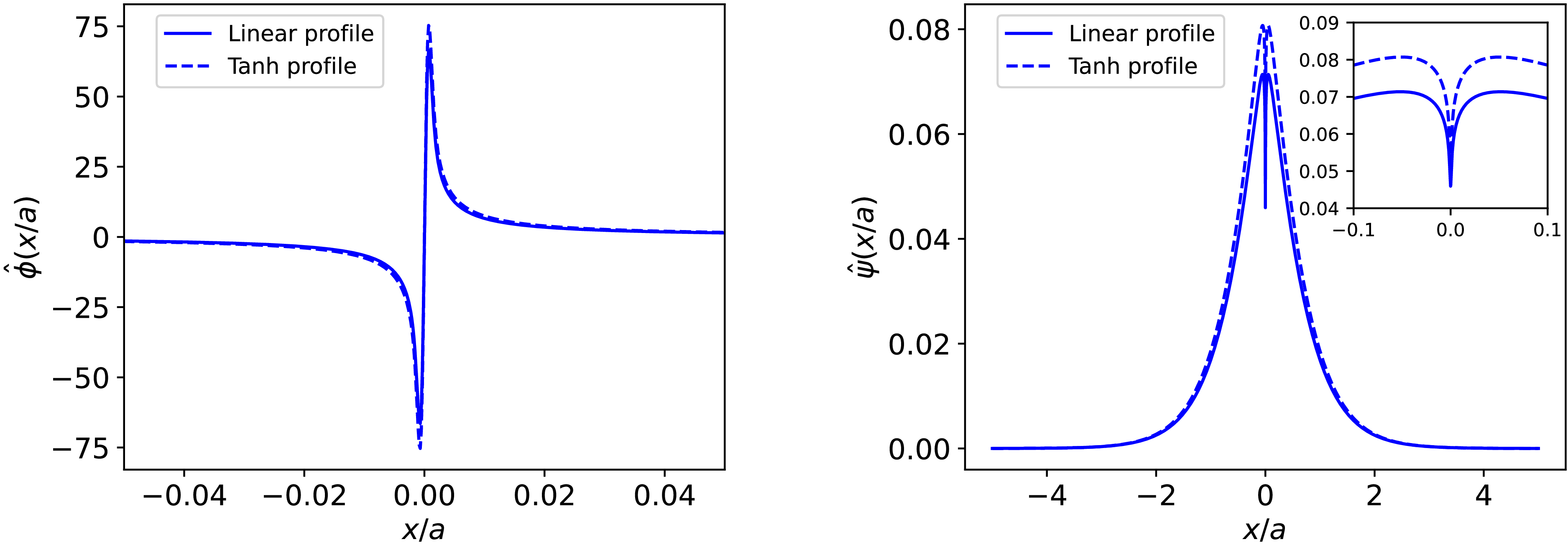
attains its largest amplitude in the limit of no stratification. The eigenfunctions of the G-mode for
 $S = 10^9$
,
 $A=0.1$
and
 $\hat {k} = 2.0$
are shown in figure 7. It can be seen that both the flux and stream functions are very localised around the singular layer and have the same parity as the tearing mode. Finally, in both modes, the
 $\tanh$
profile has a slightly higher amplitude than the linear profile in the
 $A\gt 0$
case.
Numerically solved normalised tearing-mode eigenfunctions for
 $S = 10^7$
and
 $ka = 0.5$
for three values of
 $A$
: velocity field stream function
 $\hat {\phi }$
(left-hand panel) and magnetic field flux function
 $\hat {\psi }$
(right-hand panel).

Numerically solved normalised G-mode eigenfunctions for
 $S = 10^9$
,
 $ka = 2.0$
and
 $A=0.1$
: velocity field stream function
 $\hat {\phi }$
(left-hand panel) and magnetic field flux function
 $\hat {\psi }$
(right-hand panel).

Figure 7. Long description
Two line graphs compare velocity field stream function and magnetic field flux function. Panel A: The line graph shows the velocity field stream function. The x-axis is labeled x/a and ranges from -0.04 to 0.04. The y-axis is labeled φdot a(x/a) and ranges from -75 to 75. Two profiles, Linear profile and Tanh profile, are plotted. Panel B: The line graph shows the magnetic field flux function. The x-axis is labeled x/a and ranges from -4 to 4. The y-axis is labeled φ(x/a) and ranges from 0 to 0.08. Two profiles, Linear profile and Tanh profile, are plotted. An inset zooms in on the range from -0.1 to 0.1 on the x-axis.
4.3. Scaling laws with
 $S$

As shown in previous sections, stratification has a significant effect only at large wave vectors and has minimal influence at small wave vectors when a realistic density profile is adopted. It is also well established in classical tearing theory that the constant-
 $\psi$
regime is characterised by
 $\omega \ll 1$
, whereas
 $\omega \sim 1$
in the non-constant-
 $\psi$
regime. In this sense, stratification effects are negligible in the non-constant-
 $\psi$
regime, since
 $|A|\ll 1$
. These observations motivate us to focus on the case
 $\omega \ll 1$
and
 $\hat {k}^{2}\gt A$
, for which the analytic dispersion relation is valid for both
 $A\geq 0$
and
 $A\lt 0$
, in order to determine how the scaling of the growth rate changes with
 $S$
as a result of the presence of stratification. The analytical dispersion relation given in (3.19) will admit a well-defined power law when specific asymptotic limits of
 $A$
and
 $\omega$
are considered. In what follows, we apply the simultaneous limits
 $\omega \ll 1$
and
 $|A|\ll 1$
, along with
 $S\rightarrow \infty$
to only the left-hand side of (3.19). Since the right-hand side does not depend on
 $S$
, it will not contribute to the scaling of
 $\gamma \tau _a$
with
 $S$
. A complete derivation of the scaling laws is reported in Appendix C and the main results are summarised below.
In the regime
 $|A| \ll \omega \ll 1$
, the growth rate scales as
 $\gamma \tau _a \sim S^{-3/5}$
, thus recovering the known constant-
 $\psi$
scaling law. Conversely, in the limit
 $\omega \ll |A|\ll 1$
, the scaling changes to
 $\gamma \tau _a \sim S^{-1}$
, which means the instability becomes diffusive. As noted in Appendix C, this regime exists only for
 $A\lt 0$
. Finally, when
 $A\approx \omega \ll 1$
and
 $A\gt 0$
, the growth rate
 $\gamma \tau _a \sim S^{-1/3}$
, recovering the resistive G-mode scaling. We therefore conclude that the inclusion of stratification bounds the scaling laws of the growth rate between two limiting values, namely
 $\gamma \tau _a\sim S^{-1}$
and
 $\gamma \tau _a\sim S^{-1/3}$
. Furthermore, for a finite and fixed value of
 $A$
and increasing values of the Lundquist number, the constant-
 $\psi$
tearing-mode regime will transition towards a slow diffusive mode if
 $A\lt 0$
or to the G-mode, which is a rapidly growing reconnecting mode.
The slope of the logarithm of
 $\gamma \tau _a$
as a function of the logarithm
 $S$
, obtained from numerical solution, for different stable and unstable stratification levels and
 $ka = 0.5$
. The blue dotted lines denote the reference scaling
 ${\rm d}\log(\gamma \tau _{a})/{\rm d}\log(S) = -1, -3/5, -1/3$
, ordered from bottom to top. Solid lines correspond to the linear density profile and dashed lines to the hyperbolic tangent profile.

Figure 8 presents numerically how the slope of
 $\log \hat \gamma$
as a function of
 $\log S$
varies for different stratification values. We find that the power-law scaling asymptotes to
 $\gamma \tau _{a}\sim S^{-1}$
if
 $A\lt 0$
and
 $\gamma \tau _{a}\sim S^{-1/3}$
if
 $A\gt 0$
as predicted, while if
 $A = 0$
the growth rate scales as
 $\gamma \tau _{a}\sim S^{-3/5}$
. Moreover, our results are in agreement with the weak and strong stable stratification regimes studied by Hopper et al. (Reference Hopper, Wood and Bushby2024). Notably, the
 $\tanh$
density profile displays the same predicted trends.
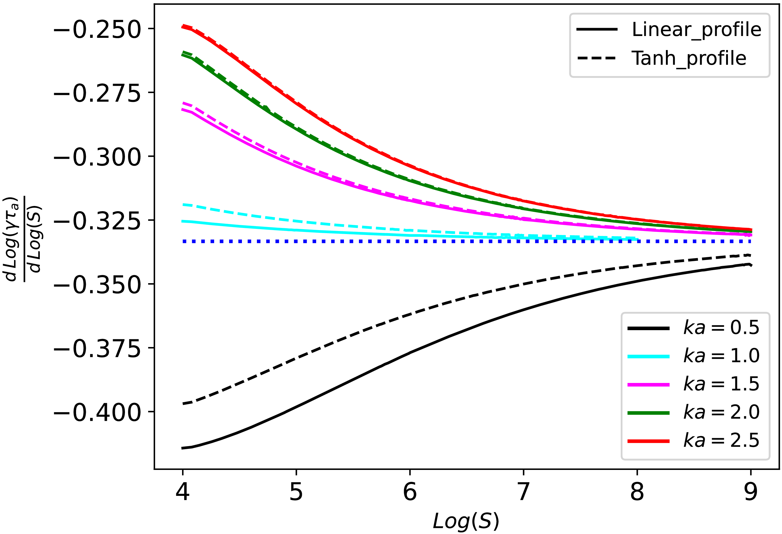
The slope of the logarithm of
 $\gamma \tau _a$
as a function of the logarithm
 $S$
, determined from numerical solution, in the large stratification limit (i.e.
 $A = 0.1$
) for different wave vectors. The blue dotted line shows the reference scaling
 ${\rm d}\log(\gamma \tau _{a})/{\rm d}\log(S)=-1/3$
.

Figure 9. Long description
A line graph with the horizontal axis labeled as Log(S) and the vertical axis labeled as dLog(vTa)/dLog(S). The graph includes multiple lines representing different values of ka, specifically ka equals 0.5, 1.0, 1.5, 2.0, and 2.5. Solid lines represent the Linear_profile, while dashed lines represent the Tanh_profile. The lines show varying trends, with some decreasing and others increasing as Log(S) increases. The blue dotted line indicates the reference scaling.
In the favourable stratification asymptotic regime, the tearing-mode growth rate scales as
 $\gamma \tau _A \sim S^{-1}$
, implying that the instability grows on the same time scale as the resistive diffusion of the equilibrium current sheet,
 $\tau _R = S\tau _A$
. This result has an important implication for the interpretation of the instability. In standard linear tearing theory, the equilibrium magnetic field is assumed to evolve resistively much more slowly than the instability growth, allowing the equilibrium to be treated as effectively fixed (quasi-static) during the linear phase. However, when
 $\gamma \tau _A \sim S^{-1}$
, this assumption is no longer satisfied because resistive diffusion and instability growth occur at comparable rates. As a result, the equilibrium evolution can no longer be neglected, and the validity of the classical linear tearing framework becomes questionable in this asymptotic limit. This behaviour suggests that favourable stratification suppresses the tearing instability so strongly that its growth becomes extremely slow, approaching a marginal regime in which the instability competes directly with resistive diffusion of the current sheet. Therefore, a more self-consistent treatment that includes the resistive evolution of the equilibrium may be required to accurately describe the system dynamics.
It is also interesting to compare the growth rate scaling with
 $S$
for the tearing and G-modes in the unstable stratification limit (
 $A\gt 0$
), shown in figure 9 for
 $A=0.1$
and different wave vectors. It can be noticed that as
 $S$
increases, the power law of the growth rate for a given wave vector becomes closer and closer to the value
 $-1/3$
in both the linear and
 $\tanh$
density profile. Specifically, for the tearing mode (
 $\hat {k}\lesssim 1$
), the stratification significantly alters the scaling of the constant-
 $\psi$
regime, gradually changing it from
 $\gamma \tau _{a} \sim S^{-3/5}$
to
 $\gamma \tau _{a} \sim S^{-1/3}$
. The same asymptotic power law of
 $-1/3$
is reached for larger wave vectors (
 $\hat {k}\gt 1$
), consistent with the well-established scaling law of the G-mode (Furth et al. Reference Furth, Killeen and Rosenbluth1963). This indicates that for a fixed value of
 $A\gt 0$
, the gravity-modified tearing mode progressively transitions to the G-mode as
 $S$
increases. In other words, the constant-
 $\psi$
regime effectively does not exist, even for weak unfavourable stratification, when
 $S\gg 1$
. A useful estimate for the onset of stratification effects can be obtained from the crossover condition (
 $|A| \sim \omega$
), which separates the weak-stratification regime (
 $|A| \ll \omega$
), for which the classical constant-
 $\psi$
tearing scaling is recovered, from the stratification-modified regime discussed in Appendix C. Using the classical constant-
 $\psi$
tearing scaling,
 $\gamma \tau _a\sim S^{-3/5}(\Delta ' a)^{4/5}(ka)^{2/5}$
, we obtain the following estimate for the crossover value of the stratification parameter:
 \begin{align} A_{\mathrm{crit}}\sim S^{-2/5}(ka)^{-2/5}(\Delta 'a)^{6/5}. \end{align}
This result implies that the threshold decreases with increasing Lundquist number, explaining why even weak stratification can significantly modify the tearing growth rate at sufficiently large S, as illustrated in figure 8.
5. Summary and conclusions
In this paper, we carried out a linear stability analysis of a slab current sheet by including a gravitational acceleration acting normal to the current layer, and studied how density stratification and gravity influence the equilibrium stability in both favourable and unfavourable density configurations. We first derived the linearised equations for the perturbed velocity and magnetic field assuming a constant density gradient, and obtained the dispersion relation through asymptotic matching of the outer and inner solutions. These analytical predictions were then compared with numerical solutions of the full eigenvalue problem. To determine how the instability depends on the assumed density model, we also introduced a more realistic hyperbolic tangent density profile and compared the resulting growth rate with the theoretical predictions. Our main findings are summarised below.
Favourable stratification (
 $A\lt 0$
) suppresses perturbations and enhances the stability of the tearing mode. As
 $|A|$
increases, the growth rate decreases, the range of unstable modes narrows and the fastest-growing mode shifts towards smaller wavelengths.
Unfavourable stratification (
 $A\gt 0$
) qualitatively changes the structure of the outer solution: solutions transition from oscillatory behaviour for
 $\hat {k}^{2} \lt A$
to exponential localisation as
 $|x| \to \infty$
for
 $\hat {k}^{2} \gt A$
. The growth rate increases with
 $A$
and the unstable spectrum extends to the G-mode regime at
 $\hat {k}\gt 1$
. We found a mismatch for
 $\hat {k}^2\lesssim A$
between analytical and numerical results for the linear density profile, due to the unlimited extent of the constant density gradient. This inconsistency is removed when using a smooth hyperbolic tangent profile, which approaches constant density away from the current layer.
For the
 $\tanh$
density profile, the dependence of the growth rate on stratification closely matches that obtained with the linear profile. Favourable stratification again reduces the growth rate and narrows the unstable spectrum. In the unfavourable case, the dispersion relation remains regular across
 $\hat {k}^{2} = A$
, and stratification primarily affects the large-
 $\hat{k}$
behaviour. For
 $\hat {k}^{2} \gt A$
, numerical results agree well with analytical predictions: stratification causes a gravity-modified tearing regime for
 $\hat {k} \lesssim 1$
that transitions smoothly into the resistive G-mode. This transition occurs once gravitational and stratification effects dominate, destabilising the resistive G-mode for
 $\hat {k} \gt 1$
. In both favourable and unfavourable regimes, the maximum growth rate and corresponding wave vector show only weak dependence on the stratification strength.
To understand the transition from tearing to G-modes, we investigated the growth rate scaling with
 $S$
for different stratification regimes by using the analytical dispersion relation, and compared predictions with numerical results. We found that the known constant-
 $\psi$
scaling
 $\gamma \tau _{a}\sim S^{-3/5}$
is recovered provided stratification becomes weaker for increasing
 $S$
(
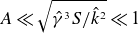 $A\ll \sqrt {\hat \gamma ^3 S/\hat{k}^{2}}\ll 1$
). For a finite stratification parameter
 $A$
, however, the growth rate admits two asymptotic limits that provide a lower and upper bound to the growth rate, namely
 $\gamma \tau _{a}\sim S^{-1}$
for
 $A\lt 0$
and
 $\gamma \tau _{a}\sim S^{-1/3}$
for
 $A\gt 0$
.
In conclusion, a favourable stratification suppresses reconnection, while unfavourable stratification only allows for rapidly reconnecting modes with
 $\gamma \tau _{a}\sim S^{-1/3}$
, namely the gravity-driven G-mode and the non-constant
 $\psi$
. In this work we have neglected physical effects that become non-negligible when dispersive or kinetic scales are reached, possibly modifying the dispersion relation at large wave vectors, or when considering microscopic current sheets. Investigating these extensions will be the subject of future work.
Acknowledgements
We wish to thank S.J. Hopper for useful discussions on the solution of the layer equations.
Editor Dmitri Uzdensky thanks the referees for their advice in evaluating this article.
Funding
We acknowledge support by DoE grant DE-FG02-04ER54742 and NSF award 2108320.
Declaration of interests
The authors report no conflict of interest.
Appendix A. Solution of the outer equation
The general solution of (3.3) in the vicinity of the boundary layer (
 $|\hat {x}|\rightarrow 0$
) is a linear combination of two power series determined via Frobenius expansion as follows:
 \begin{align} \hat {\phi }(\hat {x}) = c_{1}\hat {x}^{-l-({1}/{2})} +c_{2} \hat {x}^{l-({1}/{2})}, \end{align}
where
 $l = \sqrt {( {1}/{4})-A}$
and
 $c_{1}$
and
 $c_{2}$
are two constants to be determined by matching with the limit
 $|\hat x|\rightarrow 0$
of the complete solution. Following the method of Hopper et al. (Reference Hopper, Wood and Bushby2024) in order to get the complete solution of the outer equation (3.3) we apply the transformation
 $T = \tanh ^2(\hat {x})$
, leading to the following equation:
 \begin{align} \frac {d^{2}\hat {\phi }}{{\rm d}T^{2}}+\left (\frac {3/2}{T(1-T)}-\frac {5/2}{(1-T)}\right )\frac {{\rm d}\hat {\phi }}{{\rm d}T}-\frac {\nu ^{2}T +\left(l^{2}-\frac {1}{4}\right)(1-T)}{4T^{2}(1-T)^{2}}\hat {\phi } =0, \end{align}
with
 $\nu = \sqrt {\hat {k}^{2}-A}$
. Since this equation has three regular singular points at
 $0,\ 1$
and
 $\infty$
, it can be recast into the standard form of the hypergeometric differential equation through an appropriate change of variables as follows:
 \begin{align} \hat {\phi }(T) = T^{p} (1-T)^{q}W(T). \end{align}
With some algebra, we obtain
 \begin{align} T(1-T)W^{\prime \prime }+\left [\left(2p+\frac {3}{2}\right)-\left(2p+2q+\frac {5}{2}\right)T\right ]W^{\prime }-\left [(p+q)^{2}+\frac {3}{2}(p+q)\right ]W=0, \end{align}
which possesses the following constraints:
 \begin{align} q^{2}- \frac {\nu ^{2}}{4} &= 0;& p^{2}+\frac {p}{2}-\frac {1}{4}\left (l^{2}-\frac {1}{4}\right ) = 0. \end{align}
The solution of (3.3) is sought near the singular point
 $T=1$
(
 $\hat {x}=\infty$
) to ensure it is well behaved or convergent as
 $\hat {x}\rightarrow \infty$
. Near this singular point the solution takes the form
 \begin{align} \hat {\phi }\left (\hat {x}\right )&= T^{({l}/{2})-({1}/{4})} \left (1-T\right )^{ {\nu }/{2}}\,_{2}F_{1}\left (\frac {\nu }{2}+\frac {l}{2}-\frac {1}{4}, \frac {\nu }{2}+\frac {l}{2}+\frac {5}{4}, 1+\nu ,1-T\right )\nonumber \\[6pt]& \quad +\alpha _{2}T^{({l}/{2})-({1}/{4})}\left (1-T\right )^{- {\nu }/{2}}\,_{2}F_{1}\left (\frac {l}{2}-\frac {\nu }{2}-\frac {1}{4},\frac {l}{2}-\frac {\nu }{2}+\frac {5}{4},1-\nu ,1-T\right )\mathrm{sgn}(\hat {x}), \end{align}
where
 $\alpha _{2}$
is an arbitrary constant and
 $\,\mathrm{sgn}(\hat {x})$
ensures antisymmetry. Given that the parameter
 $\nu$
may be real or imaginary depending on the values of
 $A$
and
 $\hat {k}^2$
, it is necessary to analyse the asymptotic behaviour of the obtained solution (A6) as
 $|\hat {x}| \rightarrow \infty$
separately for each case: if
 $\hat {k}^2\gt A$
, then
 $\nu$
is purely real and only the first term of (A6) is retained, as it is well behaved in the limit
 $|\hat {x}| \rightarrow \infty$
:
 \begin{align} \hat {\phi }(\hat {x})= T^{({l}/{2})-({1}/{4})}\left (1-T\right )^{ {\nu }/{2}}\,_2F_1 \left (\frac {l}{2}+\frac {\nu }{2}-\frac {1}{4},\frac {l}{2}+\frac {\nu }{2}+\frac {5}{4},1+\nu ,1-T\right )\,\,\mathrm{sgn}(\hat {x}). \end{align}
On the other hand, when
 $\hat {k}^2\lt A$
, the parameter
 $\nu$
becomes purely imaginary. But the flow function is a real-valued function, and hence its Fourier coefficients must satisfy Hermitian symmetry (i.e.
 $\hat {\phi }^{*}(\hat {k}) = \hat {\phi }(-\hat {k})$
). As a result, we must retain both terms in (A6), with
 $\alpha _{2}$
fixed to one, to capture the full behaviour of the solution:
 \begin{align} \hat {\phi }(\hat {x})&= \Bigg [T^{({l}/{2})-({1}/{4})} (1-T)^{ {\nu }/{2}}\,_{2}F_{1}\left (\frac {\nu }{2}+\frac {l}{2}-\frac {1}{4}, \frac {\nu }{2}+\frac {l}{2}+\frac {5}{4}, 1+\nu ,1-T\right )\nonumber \\& \quad +T^{({l}/{2})-({1}/{4})} (1-T)^{- {\nu }/{2}}\,_{2}F_{1}\left (\frac {l}{2}-\frac {\nu }{2}-\frac {1}{4},\frac {l}{2}-\frac {\nu }{2}+\frac {5}{4},1-\nu ,1-T\right )\!\Bigg ]\,\mathrm{sgn}(\hat {x}). \end{align}
We now make use of the following connection formula for the hypergeometric function to relate the solution around
 $T=1$
(
 $\hat x=\infty$
) to the solution around
 $T=0$
(
 $\hat x=0$
):
 \begin{align} \,_2F_1(a,b;c;z) & = \frac {\varGamma (c)\varGamma (c-a-b)}{\varGamma (c-a)\varGamma (c-b)}\,_2F_1(a,b;a+b+1-c;1-z)\nonumber \\[6pt]& \quad +\frac {\varGamma (c)\varGamma (a+b-c)}{\varGamma (a)\varGamma (b)}(1-z)^{c-a-b}\,_2F_1(c-a,c-b;1+c-a-b;1-z). \end{align}
Finally, with the following series expansion (Abramowitz & Stegun Reference Abramowitz and Stegun1965):
 \begin{align} \,_2F_1(a,b;c;z)= \sum _{n=0}^{n=\infty }\frac {(a)_{n} (b)_{n}}{(c)_{n}}\frac {z^{n}}{n!} = \frac {\varGamma (c)}{\varGamma (a)\varGamma (b)} \sum _{n=0}^{n=\infty }\frac {\varGamma (a+n)\varGamma (b+n)}{\varGamma (c+n)} \frac {z^{n}}{n!}, \end{align}
the outer-layer solution (A7) can be written in the following series form:
 \begin{align} \hat {\phi }(\hat {x})= \sum _{n=0}^{\infty }\left [a_n |T|^{n-({l}/{2})-({1}/{4})}+b_n |T|^{n+({l}/{2})-({1}/{4})}\right ]\left (1-T\right )^{ {\nu }/{2}}\,\mathrm{sgn}(\hat {x}), \end{align}
where the coefficients
 $a_n$
and
 $b_n$
are given by
 \begin{align} a_{n} & = \frac {\varGamma (1+\nu )\varGamma (l)}{\varGamma \!\left(\frac {\nu }{2}+\frac {l}{2}+\frac {5}{4}\right)\varGamma \!\left(\frac {\nu }{2}+\frac {l}{2}-\frac {1}{4}\right)}\frac {\varGamma (1-l)}{\varGamma \!\left(\frac {\nu }{2}-\frac {l}{2}+\frac {5}{4}\right)\varGamma \!\left(\frac {\nu }{2}-\frac {l}{2}-\frac {1}{4}\right)} \nonumber\\[7pt] &\quad \times \frac {\varGamma \!\left(\frac {\nu }{2}-\frac {l}{2}+\frac {5}{4}+n\right)\varGamma \!\left(\frac {\nu }{2}-\frac {l}{2}-\frac {1}{4}+n\right)}{\varGamma (1-l+n)n!}, \end{align}
 \begin{align} b_{n} & = \frac {\varGamma (1+\nu )\varGamma (-l)}{\varGamma \!\left(\frac {\nu }{2}-\frac {l}{2}+\frac {5}{4}\right)\varGamma \!\left(\frac {\nu }{2}-\frac {l}{2}-\frac {1}{4}\right)}\frac {\varGamma (l+1)}{\varGamma \!\left(\frac {\nu }{2}+\frac {l}{2}+\frac {5}{4}\right)\varGamma \!\left(\frac {\nu }{2}+\frac {l}{2}-\frac {1}{4}\right)} \nonumber\\[7pt] & \quad\times \frac {\varGamma \!\left(\frac {\nu }{2}+\frac {l}{2}+\frac {5}{4}+n\right)\varGamma \!\left(\frac {\nu }{2}+\frac {l}{2}-\frac {1}{4}+n\right)}{\varGamma (l+1+n)n!}. \end{align}
In the immediate vicinity of the inner layer, this solution reduces to
 \begin{align} \hat {\phi }(\hat {x})= \left [a_{0} |\hat {x}|^{-l-({1}/{2})}+b_{0} |\hat {x}|^{l-({1}/{2})}\right ]\,\mathrm{sgn}(\hat {x}), \end{align}
with
 \begin{align} a_{0} = \frac {\varGamma (1+\nu )\varGamma (l)}{\varGamma \!\left(\frac {\nu }{2}+\frac {l}{2}+\frac {5}{4}\right)\varGamma \!\left(\frac {\nu }{2}+\frac {l}{2}-\frac {1}{4}\right)}, \end{align}
 \begin{align} b_{0} = \frac {\varGamma (1+\nu )\varGamma (-l)}{\varGamma \!\left(\frac {\nu }{2}-\frac {l}{2}+\frac {5}{4}\right)\varGamma \!\left(\frac {\nu }{2}-\frac {l}{2}-\frac {1}{4}\right)}. \end{align}
By comparing (A14), with (A15) and (A16), with the one obtained from the Frobenius expansion, equation (A1), enables us to determine the constants
 $c_{1}$
and
 $c_{2}$
, namely
 $c_1={a_{0}}$
and
 $c_{2}=b_{0}$
. We keep in mind that when
 $\hat {k}^2 \lt A$
, these coefficients are modified due to the contribution of the second term that was dropped for
 $\hat {k}^2 \gt A$
. Repeating the same steps for the
 $\hat {k}^2 \lt A$
case leads to the following outer solution:
 \begin{align} \hat {\phi }(\hat {x})= \left [a_{0mod} |\hat {x}|^{-l-({1}/{2})}+b_{0mod} |\hat {x}|^{l-({1}/{2})}\right ]\,\mathrm{sgn}(\hat {x}), \end{align}
where the coefficients
 $a_{0mod}$
and
 $b_{0mod}$
take the form
 \begin{align} a_{0 mod} = \frac {\varGamma (1+\nu )\varGamma (l)}{\varGamma \!\left(\frac {\nu }{2}+\frac {l}{2}+\frac {5}{4}\right)\varGamma \!\left(\frac {\nu }{2}+\frac {l}{2}-\frac {1}{4}\right)}+\frac {\varGamma (1-\nu )\varGamma (l)}{\varGamma \!\left(-\frac {\nu }{2}+\frac {l}{2}+\frac {5}{4}\right)\varGamma \!\left(-\frac {\nu }{2}+\frac {l}{2}-\frac {1}{4}\right)}, \end{align}
 \begin{align} b_{0mod} = \frac {\varGamma (1+\nu )\varGamma (-l)}{\varGamma \!\left(\frac {\nu }{2}-\frac {l}{2}+\frac {5}{4}\right)\varGamma \!\left(\frac {\nu }{2}-\frac {l}{2}-\frac {1}{4}\right)}+\frac {\varGamma (1-\nu )\varGamma (-l)}{\varGamma \!\left(-\frac {\nu }{2}-\frac {l}{2}+\frac {5}{4}\right)\varGamma \!\left(-\frac {\nu }{2}-\frac {l}{2}-\frac {1}{4}\right)}. \end{align}
Appendix B. Solution of the inner equation
We first introduce the Fourier transform in the following form:
 \begin{align} \hat {\psi } (\hat {x}) = \frac {1}{2 \pi } \int _{-\infty }^{\infty } \tilde {\psi }(\hat {\theta }) {e}^{{i} \hat {\theta }\hat {x}}\, {\rm d}\hat {\theta }, \end{align}
 \begin{align} \hat {\phi } (\hat {x}) = \frac {1}{2 \pi } \int _{-\infty }^{\infty } \tilde {\phi }(\hat {\theta }) {e}^{{i} \hat {\theta }\hat {x}}\, {\rm d}\hat {\theta }. \end{align}
Upon applying this transform, the differential equations (3.11)–(3.12) take the following form:
 \begin{align} \hat {\gamma } S \left (\tilde {\psi } - {i} \frac {\partial }{\partial \hat {\theta }} \tilde {\phi }\right ) = - \hat {\theta }^{2} \tilde {\psi }, \end{align}
 \begin{align} \left (\hat {\theta }^{2} - A \frac {\hat {k}^{2}}{\hat {\gamma }^{2}}\right ) \tilde {\phi } = - {i} \frac {\hat {k}^{2}}{\hat {\gamma }^{2}} \frac {\partial }{\partial \hat {\theta }} (\hat {\theta }^{2} \tilde {\psi }), \end{align}
and inserting equation (B3) into equation (B4) yields
 \begin{align} \frac {\hat {k}^{2}}{\hat {\gamma }} S \frac {\rm d}{{\rm d}\hat {\theta }}\left (\frac {\hat {\theta }^{2}}{\hat {\gamma }S + \hat {\theta }^{2}} \frac {{\rm d}\tilde {\phi }}{{\rm d}\hat {\theta }}\right )-\left (\hat {\theta }^{2} - A \frac {\hat {k}^{2}}{\hat {\gamma }^{2}}\right ) \tilde {\phi } = 0. \end{align}
The general solution of this equation near the edge of the boundary layer (
 $|\hat {\theta }|\rightarrow 0$
) is a linear combination of two power series determined via Frobenius expansion and is given by
 \begin{align} \tilde {\phi }(\hat {\theta }) =(\hat {k}S)^{-({l}/{3})+({1}/{6})}d_{1}\hat {\theta }^{l-({1}/{2})}+(\hat {k}S)^{({l}/{3})+({1}/{6})}d_{2}\hat {\theta }^{-l-({1}/{2})}, \end{align}
where
 $d_{1}$
and
 $d_{2}$
are two constants to be determined by matching with the limit
 $|\hat {\theta }|\rightarrow 0$
of the complete inner solution. Following the method of Shanin & Craster (Reference Shanin and Craster2002) and Hopper et al. (Reference Hopper, Wood and Bushby2024), in order to obtain the complete solution of the inner equation (B5) we introduce a new independent variable
 $\chi =\sqrt {\frac {\hat {\gamma }/S}{\hat {k}^2}}\hat {\theta }^{2}$
which yields the following equation:
 \begin{align} 4\chi ^{1/2}\frac {\rm d}{{\rm d}\chi }\left (\frac {\chi ^{3/2}}{\chi +\omega }\frac {{\rm d}\tilde {\phi }}{{\rm d}\chi }\right )- \left (\chi +\frac {l^{2}-\frac {1}{4}}{\omega }\right )\tilde {\phi }=0, \end{align}
where
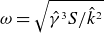 $\omega = \sqrt {{\hat {\gamma }^{3}S}/{\hat {k}^{2}}}$
.
Applying the following transformation:
 \begin{align} \tilde {\phi }(\chi ) = {\rm e}^{-({\chi }/{2})}\chi ^{({l}/{2})-({1}/{4})} Z(\chi ) \end{align}
to (B7) gives
 \begin{align} Z''(\chi ) + \left (\frac {1+l}{\chi }-1-\frac {1}{\chi +\omega }\right )\!Z'(\chi )- \frac {\left (l+\omega -\frac {1}{2}\right )}{2\chi }\! \left [\frac {l+\omega +\frac {1}{2}}{2\omega }+\frac {1}{\chi +\omega }\right ]Z(\chi ) =0, \end{align}
where the prime denotes differentiation with respect to
 $\chi$
. Shanin & Craster (Reference Shanin and Craster2002) have provided solutions for this class of ordinary differential equations. Accordingly, following their approach, the general solution of (B7) can thus be expressed in terms of the confluent hypergeometric function
 $U(a,b,z)$
as
 \begin{align} \tilde {\phi } (\chi )= {\rm e}^{-({\chi}/{2})} \chi ^{({l}/{2})-({1}/{4})} &\Bigg [U\left (\frac {(l+\omega )^{2}-\frac {1}{4}}{4\omega },1+l,\chi \right )\nonumber\\[7pt]& +\left (\frac {(\omega -\frac {1}{2})^{2}-l^{2}}{4\omega }\right )U\left (\frac {(l+\omega )^{2}-\frac {1}{4}}{4\omega }+1,1+l,\chi \right )\Bigg ]\,\mathrm{sgn}(\hat {\theta }). \end{align}
Using Kummer’s transformation for the Tricomi function
 $U(a,b,z)$
and noting that Kummer’s function
 $M(a,b,z)$
in fact is a generalised hypergeometric series of the form
 \begin{align} U(a,b,z) = \frac {\varGamma (1-b)}{\varGamma (a-b+1)}M(a,b,z)+\frac {\varGamma (b-1)}{\varGamma (a)}z^{1-b}M(a-b+1,2-b,z), \end{align}
 \begin{align} M(a,b,z) =\sum _{n=0}^{\infty }\frac {(a)_{n}}{(b)_{n}n!}z^{n} = 1 + \frac {a}{b}z+\frac {a(a+1)}{b(b+1)2!}z^{2}+\cdots , \end{align}
then the series representation of the solution (B10) in the limit
 $\hat {\theta }\rightarrow 0$
can be expressed as
 \begin{align} \tilde {\phi }(\hat {\theta })= \big[\tilde {a}_{0}|\hat {\theta }|^{l-({1}/{2})}+\tilde {b}_{0}|\hat {\theta }|^{-l-({1}/{2})}\big]\,\mathrm{sgn}(\hat {\theta }), \end{align}
where the coefficients
 $\tilde {a}_{0}$
and
 $\tilde {b}_{0}$
are
 \begin{align} \tilde {a}_{0}=\left ({\frac {\sqrt {\hat {\gamma }/S}}{\hat {k}}}\right )^{({l}/{2})-({1}/{4})}\frac {2\omega }{\left(\omega -l+\frac {1}{2}\right)}\frac {\varGamma (-l)}{\varGamma \left (\left({(\omega -l)^{2}-\frac {1}{4}}\right)/{4\omega }\right )}, \end{align}
 \begin{align} \tilde {b}_{0}=\left ({\frac {\sqrt {\hat {\gamma }/S}}{\hat {k}}}\right )^{-({l}/{2})-({1}/{4})}\frac {2\omega }{\left(\omega +l+\frac {1}{2}\right)}\frac {\varGamma (l)}{\varGamma \left (\left({(l+\omega )^{2}-\frac {1}{4}}\right)/{4\omega }\right )}. \end{align}
By comparing (B13), with (B14)–(B15), with the solution given by the Frobenius expansion, equation (B6), allows us to determine the constants
 $d_{1}$
and
 $d_{2}$
as follows:
 \begin{align} d_{1} = (\hat {k}S)^{({l}/{3})-({1}/{6})}\left ({\frac {\sqrt {\hat {\gamma }/S}}{\hat {k}}}\right )^{({l}/{2})-({1}/{4})}\frac {2\omega }{\left(\omega -l+\frac {1}{2}\right)}\frac {\varGamma (-l)}{\varGamma \left (\left({(\omega -l)^{2}-\frac {1}{4}}\right)/{4\omega }\right )}, \end{align}
 \begin{align} d_{2} =(\hat {k}S)^{-({l}/{3})-({1}/{6})}\left ({\frac {\sqrt {\hat {\gamma }/S}}{\hat {k}}}\right )^{-({l}/{2})-({1}/{4})}\frac {2\omega }{\left(\omega +l+\frac {1}{2}\right)}\frac {\varGamma (l)}{\varGamma \left (\left({(l+\omega )^{2}-\frac {1}{4}}\right)/{4\omega }\right )}. \end{align}
Appendix C. Derivation of scaling laws
Let us rewrite the dispersion relation that is valid when
 $\hat {k}^{2}\gt A$
as follows:
 \begin{align} &\left ({\frac {\sqrt {\hat {\gamma }/S}}{\hat {k}}}\right )^{l}\frac {\left(\omega +l+\frac {1}{2}\right)}{\left(\omega -l+\frac {1}{2}\right)}\frac {\varGamma (-l)}{\varGamma (l)}\frac {\varGamma \left (\left({(\omega +l)^{2}-\frac {1}{4}}\right)/{4\omega }\right )}{\varGamma \left (\left({(\omega -l)^{2}-\frac {1}{4}}\right)/{4\omega }\right )}\nonumber\\[5pt] & \quad =\frac {\cos \left (\frac {\pi }{2}\left(\frac {1}{2}+l\right)\right )\varGamma \!\left(\frac {1}{2}-l\right)}{\cos \left (\frac {\pi }{2}\left(\frac {1}{2}-l\right)\right )\varGamma \!\left(\frac {1}{2}+l\right)}\frac {\varGamma (l)}{\varGamma (-l)}\frac {\varGamma \!\left(\frac {\nu }{2}-\frac {l}{2}+\frac {5}{4}\right)\varGamma \!\left(\frac {\nu }{2}-\frac {l}{2}-\frac {1}{4}\right)}{\varGamma \!\left(\frac {\nu }{2}+\frac {l}{2}+\frac {5}{4}\right)\varGamma \!\left(\frac {\nu }{2}+\frac {l}{2}-\frac {1}{4}\right)}. \end{align}
In the small but finite stratification limit (
 $|A|\ll 1$
), the parameter
 $l$
can be approximated as
 $l \approx ( {1}/{2})-A$
. Accordingly, the left-hand side simplifies to
 \begin{align} \left ({\frac {\hat {\gamma }}{S\hat {k}^{2}}}\right )^{ ({1}/{4})-{ ({A}/{2})}}\frac {{\omega }-A+1}{{\omega }+A}\frac {\varGamma \!\left(-\frac {1}{2}+A\right)}{\varGamma \!\left(\frac {1}{2}-A\right)}\frac {\varGamma \left (({\omega ^2-2\omega A +A^{2}+\omega -A})/{4{\omega }}\right )}{\varGamma \left (({\omega ^2+2\omega A +A^{2}-\omega -A})/{4{\omega }}\right )}. \end{align}
As we mentioned above, we want to derive the scaling laws of the growth rate with Lundquist number
 $S$
in the regimes
 $|A|\ll \omega \ll 1$
,
 $\omega \ll |A|\ll 1$
and
 $|A|\approx \omega \ll 1$
. As a result of those limits, the previous expression can be approximated by
 \begin{align} \left ({\frac {\hat {\gamma }}{S\hat {k}^{2}}}\right )^{ {1}/{4}}\frac {1}{{\omega }+A}\frac {\varGamma \!\left(-\frac {1}{2}+A\right)}{\varGamma \!\left(\frac {1}{2}-A\right)}\frac {\varGamma \!\left(\frac {1}{4}-\frac {A}{4\omega }\right)}{\varGamma \!\left(-\frac {1}{4}-\frac {A}{4\omega }\right)}, \end{align}
where the fraction
 \begin{align} \frac {\varGamma \!\left(-\frac {1}{2}+A\right)}{\varGamma \!\left(\frac {1}{2}-A\right)} \lt 0, \end{align}
for both positive and negative
 $A$
, and therefore the left-hand side carries an overall negative sign. This negative sign cancels the sign arising from the subsequent scaling.
C.1. The
$|A| \ll \omega \ll 1$
limit

In the limit
 $|A| \ll \omega \ll 1$
, we can neglect
 $A$
compared to
 $\omega$
. Thus, (C3) reduces to
 \begin{align} \left ({\frac {\hat {\gamma }}{S\hat {k}^{2}}}\right )^{ {1}/{4}}\frac {1}{{\omega }}\frac {\varGamma \!\left(-\frac {1}{2}+A\right)}{\varGamma \!\left(\frac {1}{2}-A\right)}\frac {\varGamma \!\left(\frac {1}{4}\right)}{\varGamma \!\left(-\frac {1}{4}\right)}, \end{align}
and, hence, the growth rate scales with
 $S$
as
 \begin{align} \hat {\gamma } \sim S^{-3/5}. \end{align}
C.2. The
$\omega \ll |A| \ll 1$
limit

In the limit
 $\omega \ll |A| \ll 1$
, we can neglect
 $\omega$
compared to
 $A$
. Therefore, expression (C3) takes the form
 \begin{align} \left ({\frac {\hat {\gamma }}{S\hat {k}^{2}}}\right )^{ {1}/{4}}\frac {1}{{A}}\frac {\varGamma \!\left(-\frac {1}{2}+A\right)}{\varGamma \!\left(\frac {1}{2}-A\right)}\frac {\varGamma \!\left(\frac {1}{4}-\frac {A}{4\omega }\right)}{\varGamma \!\left(-\frac {1}{4}-\frac {A}{4\omega }\right)}. \end{align}
By applying the following asymptotic expansion of the Gamma function:
 \begin{align} \frac {\varGamma (z+a)}{ \varGamma (z+b)}\thicksim z^{a-b}, \end{align}
where
 $z= {A}/{4\omega }$
, (C7) simplifies to
 \begin{align} \left ({\frac {\hat {\gamma }}{S\hat {k}^{2}}}\right )^{ {1}/{4}}\frac {1}{{A}}\frac {\varGamma \!\left(-\frac {1}{2}+A\right)}{\varGamma \!\left(\frac {1}{2}-A\right)}\left (-\frac {A}{4\omega }\right )^{ {1}/{2}}. \end{align}
As a result, this limit is valid only if
 $A\lt 0$
, with the growth rate scaling as
 \begin{align} \hat {\gamma } \sim S^{-1}. \end{align}
C.3. The
$\omega \approx |A| \ll 1$
limit,
$A\gt 0$


In this limit,
 $\omega$
is comparable to
 $A\gt 0$
. Thus, we can Taylor-expand the Gamma functions given in (C3) around
 $A/\omega =1$
to obtain
 \begin{align} \left ({\frac {\hat {\gamma }}{S\hat {k}^{2}}}\right )^{ {1}/{4}}\frac {1}{A+\omega }\frac {\varGamma \!\left(-\frac {1}{2}+A\right)}{\varGamma \!\left(\frac {1}{2}-A\right)}\frac {\omega }{A-\omega }. \end{align}
In order to have a finite value in the limit
 $S\rightarrow \infty$
, one must therefore impose that
 \begin{align} A^2\sim \omega ^{2}, \end{align}
such that the growth rate scaling becomes
 \begin{align} \hat {\gamma } \sim S^{-1/3}. \end{align}
This regime does not exist for
 $A\lt 0$
, for which (C3) tends to zero in the limit of
 $S\rightarrow \infty$
and thus a solution to (C1) for the growth rate does not exist.


 A⩽0
 S=106

 A⩾0
 S=105

 A⩽0
 S=106
 A⩾0
 S=105
 S=105
 A=0.01
 A=0

 S=107
 ka=0.5
 A
 ϕ^
 ψ^
 S=109
 ka=2.0
 A=0.1
 ϕ^
 ψ^

 γτa
 S
 ka=0.5
 dlog(γτa)/dlog(S)=−1,−3/5,−1/3
 γτa
 S
 A=0.1
 dlog(γτa)/dlog(S)=−1/3

 Open access

