As the theme for this issue of the journal is bipolar disorder (BP) we will look at power calculations for a study to examine the performance of diagnostic and screening tests for BP. Developing and evaluating such tests is of some interest as they have an important practical role in research and health service delivery. Some common uses of these tests are: (a) diagnosis in a clinical setting; (b) early detection in large groups of people at above-average risk; and (c) large-scale epidemiological studies seeking to estimate the prevalence in the population. In (a), a test typically supplements a clinical interview, in (c) it substitutes for the preferable, but impractical, clinical interview, while in (b) it can do either.

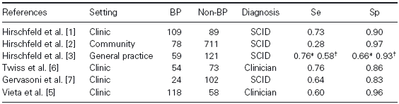
The simplest study we might do is to estimate, in our particular setting, the sensitivity (Se), which is the proportion of cases positive on a test, and the specificity (Sp), which is the proportion of non-cases negative on a test (see Reference Hadzi-Pavlovic(1)) for an introduction to these concepts). A validation study typically starts from what is known of a test. As an example we will take the Mood Disorder Questionnaire (MDQ; Reference Hirschfeld, Williams and Spitzer(2)), which appears to be the most frequently examined test for BP. In Table 1 we have listed the Se and Sp (based on all BP patients) from three studies by the authors of the MDQ (Reference Hirschfeld, Williams and Spitzer2–Reference Hirschfeld, Cass and Holt4) as well as three recent studies examining further its validity (Reference Vieta, Sánchez-Moreno and Bulbena5–Reference Gervasoni, Rouget and Miguez7). It is worth thinking about why these results differ–not that the differences are large.

Table 1

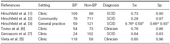
Estimates of Se and Sp of the MDQ

* Raw results.

† Adjusted for sampling and severity (see source for details).

Se, the sensitivity; Sp, the specificity.

Differences in Se (or Sp) indicate that the distribution of MDQ scores in cases (or non-cases) differs such that different proportions fall above (or below) the standard cut-off. This suggests that differing subsets of cases are being selected by the studies, though the major difference need not be one of psychopathology, but could simply be in how they respond to questionnaires. Further, different proportions of BP-I and BP-II and NOS are included under BP. Similarly, the non-BP groups differ: patients with depression in some studies, members of the community who are well in another. Diagnosis is a further source of difference: some studies used a face-to-face Structured Clinical Interview for DSM-IV (SCID); the community study used a telephone-administered SCID; while other studies had clinicians making the diagnosis. Finally, two studies used translated versions of the MDQ: one Spanish Reference Vieta, Sánchez-Moreno and Bulbena(5) and one French Reference Gervasoni, Rouget and Miguez(7).

These results in Table 1 suggest that a researcher proposing a study in a clinical setting would expect a Se of around 0.68 and a Sp of around 0.89. There are two ways to approach our question. The first is to ask what sample size we need in order to be able to express our finding as a proportion plus a range that we are highly confident includes the true value. For example, we might want to report Se = 0.80 ± 0.05 which puts Se in the range 0.75–0.85. Such a range is called a confidence interval (CI) and a 95% CI says that we are 95% confident that the interval includes the true value. The range ± 0.05 has been chosen because we require that degree of precision, perhaps because we need an accurate picture of the clinical and economic costs and benefits of our screening test.

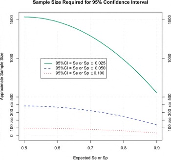
In Fig. 1 we have plotted the sample sizes required for a range of possibilities based on Table 1. There will be two sample sizes: one for Se which is the required number of cases and one for Sp which is the required number of non-cases. If we anticipate the test will have a Se = 0.8 then a sample size of around 250 is required for a CI of 0.8 ± 0.05. Of course if the literature provides a range of values (e.g. 0.65–0.75 for clinics in Table 1) then we need to consider a range of samples sizes (e.g. 350–250). In practice, the total number of cases and non-cases which needs to be recruited will depend on the prevalence of cases: if this is low one might have to recruit many more non-cases in order to have enough cases.

Fig. 1

Sample size required to set specified confidence intervals for different anticipated values of the sensitivity (Se) or the specificity (Sp).

Another question that we might ask is whether one test (Test A) differs in its Se or Sp from another (Test B). In Reference Vieta, Sánchez-Moreno and Bulbena(5), for example, the MDQ was compared to a newly developed test. Typically we do this using the same patients, that is, both tests are administered to the sample of patients, their Se and Sp determined against the diagnostic criterion, and then we want to compare the two Se and the two Sp. This comparison is usually made using McNemar's test for dependent (or paired) proportions.

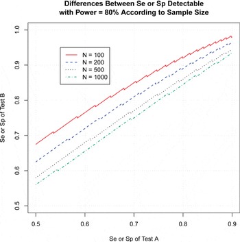
In Fig 2 we have taken some representative sample sizes (100, 200, 500 and 1000) and looked to see what size of difference for Se or Sp can be detected between Test A and Test B (where B > A). For this question we are interested to also set the power of our study, that is, to have a sufficient sample so that, if the two tests differ by the specified amount, then we can 80% (or whatever) confident of finding that difference. For example, if Test A is anticipated to have Se = 0.70 and Test B to have Se = 0.80, then we need a little over 200 patients to have 80% power to detect that difference. The jagged nature of the lines is a common feature of power calculations involving proportions.

Fig. 2

Differences in the sensitivity (Se) or the specificity (Sp) between Test A and Test B detectable with power = 80% for four different sample sizes (N = 100, 200, 500 and 1000).