1. Introduction: stratified Poiseuille flow

Plane Poiseuille flow, i.e. steady flow between two infinite parallel plates, is one of the simplest and most common shear flows. In the non-stratified case, it is known to be linearly unstable for Reynolds numbers larger than $5772$ (Orszag Reference Orszag1971). Above this value, two-dimensional (2-D) waves, known as Tollmien–Schlichting (TS) waves, are viscously unstable and can develop and propagate in the flow. We present here the stability analysis of a horizontal plane Poiseuille flow that is stably stratified in density along the vertical direction, i.e. orthogonal to the plane of the horizontal shear. As density stratification is ubiquitous in nature, the instability of this stratified flow may be relevant to water flows in submarine canyons, to winds in deep valleys or to laminar flows in rivers or canals where stratification can be due to temperature or salinity gradients.

The situation where shear is inclined versus stratification has already been studied, for instance, for jets (Candelier, Le Dizès & Millet Reference Candelier, Le Dizès and Millet2011), for a Kolmogorov shear flow (Lucas, Caulfield & Kerswell Reference Lucas, Caulfield and Kerswell2017) or for vortex dipoles (Deloncle, Chomaz & Billant Reference Deloncle, Chomaz and Billant2007). It differs from the more classical 2-D case where both stratification and shear lie in the same plane (Gage & Reid Reference Gage and Reid1968; Caulfield Reference Caulfield1994). According to the studies of Basovich & Tsimring (Reference Basovich and Tsimring1984) and Bakas & Farrell (Reference Bakas and Farrell2009a,Reference Bakas and Farrellb), horizontal shear flows can indeed excite internal gravity waves in the presence of a vertical stratification. Our study follows recent investigations on instabilities of stratified rotating or non-rotating shear flows: the strato-rotational instability in Taylor–Couette flows (Le Bars & Le Gal Reference Le Bars and Le Gal2007; Park & Billant Reference Park and Billant2013; Rüdiger et al. Reference Rüdiger, Seelig, Schultz, Gellert, Egbers and Harlander2017) or plane Couette flows (Vanneste & Yavneh Reference Vanneste and Yavneh2007; Facchini et al. Reference Facchini, Favier, Le Gal, Wang and Le Bars2018), and the radiative instability in boundary layer flows (Candelier, Le Dizès & Millet Reference Candelier, Le Dizès and Millet2012; Chen, Bai & Le Dizès Reference Chen, Bai and Le Dizès2016), rotating flows (Riedinger, Le Dizès & Meunier Reference Riedinger, Le Dizès and Meunier2011) or vortices (Le Dizès & Billant Reference Le Dizès and Billant2009; Riedinger, Le Dizès & Meunier Reference Riedinger, Le Dizès and Meunier2010). All of these examples belong to a class of instabilities caused by the resonant interaction of Doppler-shifted internal gravity waves (Molemaker, McWilliams & Yavneh Reference Molemaker, McWilliams and Yavneh2001; Le Dizès & Riedinger Reference Le Dizès and Riedinger2010).

More generally, resonances of different types of waves in shear flows are the subject of a long-standing history originating from the seminal paper of Cairns (Reference Cairns1979) on the Kelvin–Helmholtz instability, then extended to surface flows by Satomura (Reference Satomura1981) and also to different arrangements of stratified flows (see, for instance, the review by Carpenter, Tedford & Heifetz (Reference Carpenter, Tedford, Heifetz and Lawrence2011)). Even TS waves were shown to be possibly interpreted as the result of a resonant interaction of two different components (Baines, Majumdar & Mitsudera Reference Baines, Majumdar and Mitsudera1996). A particular feature of the present case is that the TS waves can themselves also interact and possibly resonate with inviscid gravity waves. But, to our knowledge, the first to realize the existence of this wave-related destabilization for continuously stratified fluids was Taylor (Reference Taylor1931), who showed that stratification – intuitively seen as a stabilizing effect – may destabilize stable parallel basic flows. Note that the phenomenon of interaction between viscous vorticity waves and gravity waves was already observed by Eaves & Caulfield (Reference Eaves and Caulfield2017) in a 2-D numerical simulations of Couette flow with a three-layer density distribution, i.e. in a case when shear and density gradients are aligned. As described by these authors, this coupling gives rise to a viscous Holmboe-wave instability. This interaction was in fact previously suggested by Lindzen & Barker (Reference Lindzen and Barker1985) through a mechanism of internal wave over-reflections at critical levels.

2. Experimental set-up and numerical methods

The experiments are realized in an annular channel having a diameter at mid-gap of $2R = 1.515$ m and a rectangular vertical section of $85\ \textrm {mm}\times 250\ \textrm {mm}$. This channel is filled up to a level $h$ chosen between $128$ and $200$ mm (position of the free surface) with linearly stratified salty (NaCl) water. The Schmidt number of the fluid, defined as the ratio of momentum diffusivity (kinematic viscosity) and mass diffusivity, is equal to $Sc = 700$. The tank is made of transparent acrylic glass (polymethyl methacrylate, PMMA) so that the fluid interior is entirely accessible to non-invasive measurement techniques such as particle image velocimetry (PIV). For tank rotation, a synchronous servomotor (model CMPZ100S) with helical-bevel gear unit (KAF57) from SEW-EURODRIVE is used. Deviations in rotation rate are less than $2\,\%$. The laser used for PIV is a Nano 250-532-100 from the Linos AG company. It is a diode-pumped steady laser that emits a monochromatic beam at a wavelength of $532$ nm. The laser beam goes through a cylindrical-lens optical system that spreads it into a 2-D plane sheet of about 1 mm thickness. For the experiments we used a mixture of two different PIV particles from DANTEC: hollow glass spheres and silver-coated hollow glass spheres. The camera used to record the flow is a GoPro HERO 4 Black. It has a video resolution of 1080p, which corresponds to a screen resolution of $1920 \times 1080$ pixels, with an image rate of $30$ or $48$ frames per second. A modification that improved the data was to change the lenses of the GoPro camera with lenses provided by The Imaging Source^®. With the updated lens we can control the focusing and the aperture, which significantly improves the quality of our PIV measurements.

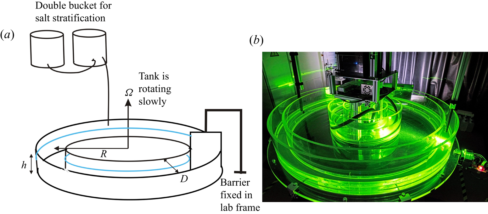
The free surface fluid is then set in motion by the side and bottom walls of the curved channel, which is slowly rotated at a rate $\varOmega$. However, a barrier ($28$ cm high, $8.4$ cm wide and $10$ mm thick plastic plate) that nearly fits the rectangular cross-section of the channel is placed along the radius inside the channel. As it is maintained stationary in the laboratory frame, this wall blocks the fluid and prohibits solid-body rotation, resulting in a nearly parabolic horizontal velocity profile. Figure 1 presents a drawing and a photograph of the installation at the Brandenburg University of Technology, Cottbus-Senftenberg.

Figure 1.

Drawing (a) and photograph (b) of the experimental installation: an annular channel of rectangular section $85\ \textrm {mm}\times 200\ \textrm {mm}$ and radius at mid-gap $R=75.75$ cm is rotated at a weak angular velocity $\varOmega$ between $0.1$ and $0.5$ r.p.m. The Poiseuille flow is created by the insertion of a barrier fixed in the laboratory frame that prohibits solid-body rotation of the fluid in the annulus.

To complement the experiments, we also perform direct numerical simulations (DNS) using the spectral element solver Nek5000 (version 19.0; Argonne National Laboratory, Illinois; available at https://nek5000.mcs.anl.gov) (Fischer Reference Fischer1997). The same equations as used to study stratified Couette flow by Facchini et al. (Reference Facchini, Favier, Le Gal, Wang and Le Bars2018) are adapted here to the Poiseuille case. A constant and uniform streamwise force is added to the momentum equation in order to reach the targeted Poiseuille flow profile by compensating for viscous dissipation. Note that this is different from the experiment, where the Poiseuille profile is maintained at zero constant mass flux instead of constant force. This does not affect the linear behaviour of the instability but might have some effect on its nonlinear development, which is outside the scope of the present paper.

We consider the simplest case of plane Poiseuille flow between two vertical walls that are static, with no slip and with zero buoyancy flux. The other directions are assumed to be periodic. In order to avoid confinement effects due to the inherent discretization of the wave vectors fitting inside our numerical domain, we consider a rather large domain of dimensionless size $(L_x,L_y,L_z)=(16,2,6)\times D/2$, where $D$ is the width of the channel, the stratification is along the vertical direction and the Poiseuille flow is along the $x$ direction. While we can reach the Reynolds and Froude numbers of the experiments, we cannot consider the same Schmidt number. We typically consider values between $1$ (as in the linear stability analysis, see § 5 below) and $7$.

3. Base flow profile

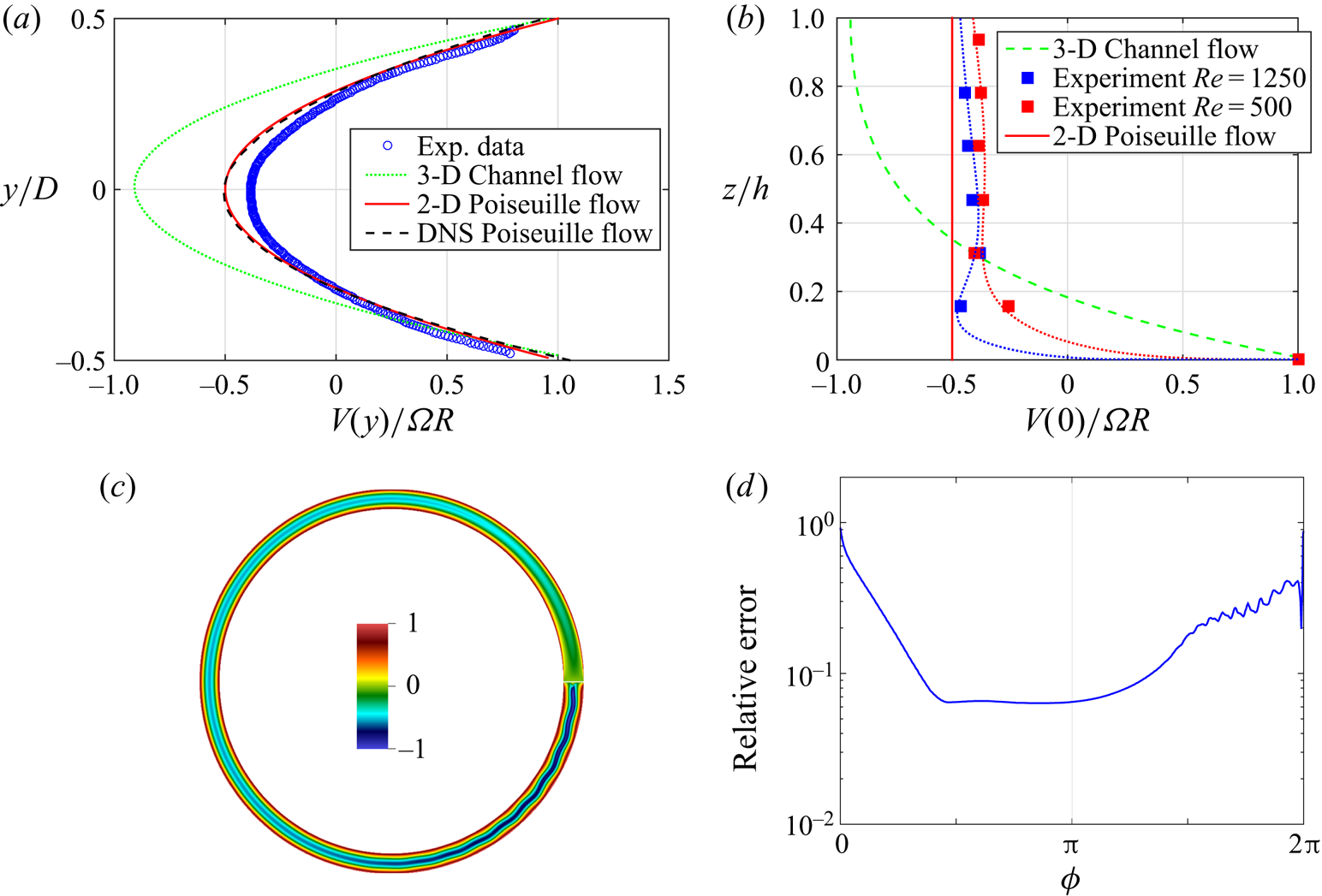
We discuss in this section the equilibrium base flow as measured in the experiments in the absence of instability. At very low velocities (i.e. under a threshold, as we will see later) and using the PIVlab software (Thielicke & Stamhuis Reference Thielicke and Stamhuis2014), PIV measurements in horizontal planes permit the base flow to be characterized at different vertical levels. Figure 2(a) shows an example of a transverse (in the radial direction of the annulus) profile of the horizontal velocity, which is compared, on the one hand, to analytically obtained parabolic 2-D plane Poiseuille flow (which does not therefore take into account the presence of the bottom), and, on the other hand, to the analytical three-dimensional (3-D) profile of the channel flow, i.e. when taking into account the shear at the bottom (see e.g. Theofilis, Duck & Owen Reference Theofilis, Duck and Owen2004). As can be seen, the experimental profile is very close to the analytical 2-D parabolic profile with a zero flux. Moreover, as presented in figure 2(b) for two PIV measurements at respectively $Re=1250$ for a Froude number $F=0.30$ and at $Re=500$ for a Froude number $F=0.12$, the vertical profiles of the horizontal velocity (see figure 2b) are very flat over most of the height of the flow. This phenomenon is due to the presence of a mixed layer at the bottom of the channel that acts somehow as a lubrication layer and restricts the velocity vertical gradient to a few centimetres at the bottom.

Figure 2.

(a) Example for a Reynolds number $Re=1250$ and a Froude number $F=0.30$ of a measured horizontal profile of the dimensionless longitudinal velocity at a height of $100$ mm (the total depth of water being $h=128$ mm) (blue circles). We also show for comparison the theoretical 2-D planar and 3-D profiles, along with the results of a 2-D DNS in the annulus. (b) Two examples of the vertical profile of the dimensionless horizontal velocity measured in the experiment at $Re=1250$ for a Froude number $F=0.30$ (blue squares) and at $Re=500$ for a Froude number $F=0.12$ (red squares); the dotted lines are there to guide the eye. These profiles can be compared to the 3-D channel flow profile (green dashed line) and to the invariant 2-D Poiseuille flow profile (red full line). (c) Visualization of the azimuthal velocity from DNS during the quasi-steady phase for $Re=2000$ in a rotating 2-D cylindrical annulus. A thin impenetrable and no-slip barrier is cutting through the annulus on the right. (d) Relative error between the radial profile of azimuthal velocity in the 2-D cylindrical annulus from DNS and the theoretical 2-D planar Poiseuille profile, as a function of the azimuthal position. The barrier is located at $\phi =0[2{\rm \pi} ]$.

As a consequence, the base flow studied here is very close to ideal 2-D laminar plane Poiseuille flow. This ideal 2-D flow profile with zero flux can be written in the laboratory frame as a function of the transverse coordinate $y$ (with its origin located at the middle of the channel) when neglecting the rotation and curvature effects: $U(y) = \varOmega R[12 (y/D)^2 - 1]/2$, where $D$ is the width of the annular channel and $R$ its radius at mid-gap. The maximum velocity is thus reached near the vertical walls: $U(\pm D/2) = \varOmega R$ and its minimum is located at the centre of the channel: $U(0)= - \varOmega R/2$. The small asymmetry between the inner and outer walls – located at different radii – is neglected. Taking $D/2$ as typical length scale and $3 \varOmega R / 2$ as typical velocity scale, we can define the Reynolds number and the Froude number of the flow as: $Re = 3\varOmega R D/4\nu$, where $\nu$ is the kinematic viscosity of the fluid, and $F = 3\varOmega R/ND$, where $N$ is the Brunt–Väisälä frequency characterizing the density stratification. To check that rotation has a negligible effect on the flow, we can calculate its Rossby number as the ratio between the local vorticity and twice the rotation rate $\varOmega$. The local vorticity, calculated from the velocity profile, is equal to $12 \varOmega R y / D^2$. Therefore, the analytical expression of the Rossby number is $6 R y/ D^2$. Its mean value across the channel is $3 R /2D$, which is as large as $13$ due to the high aspect ratio of the channel. Therefore, we can conclude that the rotation of the channel has a small effect on the flow. Note that the curvature of the channel scales in the same way and thus can be neglected for the same reason.

To support our experimental observations of the base flow in this particular arrangement, we have also computed the 2-D flow in the same geometry as that of the experiment using again Nek5000. The 2-D Navier–Stokes equations are solved inside a cylindrical annulus rotating at constant rate $\varOmega$. A static barrier with no-slip boundary conditions is inserted at an arbitrary azimuthal angle (here $\phi =0[2{\rm \pi} ]$). Starting from a fluid at rest, we wait for the system to reach a quasi-steady state represented in figure 2(c). While the expected 2-D Poiseuille profile is perturbed on both sides of the barrier, the velocity profile measured at a diametrically opposed position is very close to the theoretical 2-D planar result (see figure 2a). To be more quantitative we have also computed the relative error between the radial profile of azimuthal velocity in the 2-D cylindrical annulus and the theoretical 2-D planar Poiseuille profile, as a function of the azimuthal position $\phi$. As can be seen in figure 2(d), there is an extended plateau where this error stays smaller than $7\,\%$.

While this numerical simulation confirms that rotation and curvature effects remain negligible, the mechanism preventing the 3-D channel profile from developing in the stratified experiment remains to be explained. But we can speculate that it is due to the combined effect of stratification and localized turbulent mixing caused by leakage under the barrier. The fluid is first stratified before being slowly set into rotation. When arriving at the barrier, except near the bottom wall, the fluid particles stay at the same elevation, minimizing the energy to turn back, following in this way horizontal streamlines. Besides this effect, which bidimensionalizes the flow, we think that the fluid jet leaking through the small gap between the barrier and the bottom is mixed by turbulence. This effect decouples the bulk from the bottom wall, which as a consequence cannot transmit its momentum through viscous effects. Therefore, we can imagine that this thin layer (which grows very slowly in time) acts as a kind of lubrication layer. The precise study of this mechanism is left for a further study, since the analysis of the 2-D Poiseuille flow instability is our main focus here.

4. Experimental and numerical analysis of the instability

To explore the instability, four independent experimental runs were performed with different stratifications and heights of water in the channel. Each of these runs obeys the same protocol. First we create a linear stratified layer of a chosen total height $h$ using the classical double bucket technique (Oster Reference Oster1965). Having measured the density profile, and determined by linear fit the corresponding Brunt–Väisälä frequency, the annulus is progressively set into rotation step by step. When having reached the desired rotation rate $\varOmega$, we wait for a period of time ranging between several hours and 20 min in the cases where the velocity increments were small. 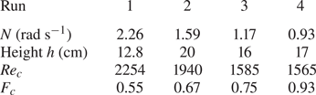Note that the critical parameters vary in each run, as the density gradient and total height $h$ are changed for each of them. Table 1 gives the principal characteristics of the experimental runs and also the values of the critical Reynolds and Froude numbers obtained from interpolations between the stable and unstable flows observed by their corresponding PIV velocity fields. The critical Reynolds numbers $Re_c$ are first determined by extrapolating the measured amplitudes of the velocity fields under and above the transition (see figure 5 later). The corresponding critical Froude numbers $F_c$ are then calculated from the estimated values of $\varOmega$ at threshold.

Table 1.

Characteristics of the four experimental runs under study with their corresponding observed instability threshold values $Re_c$ and $F_c$.

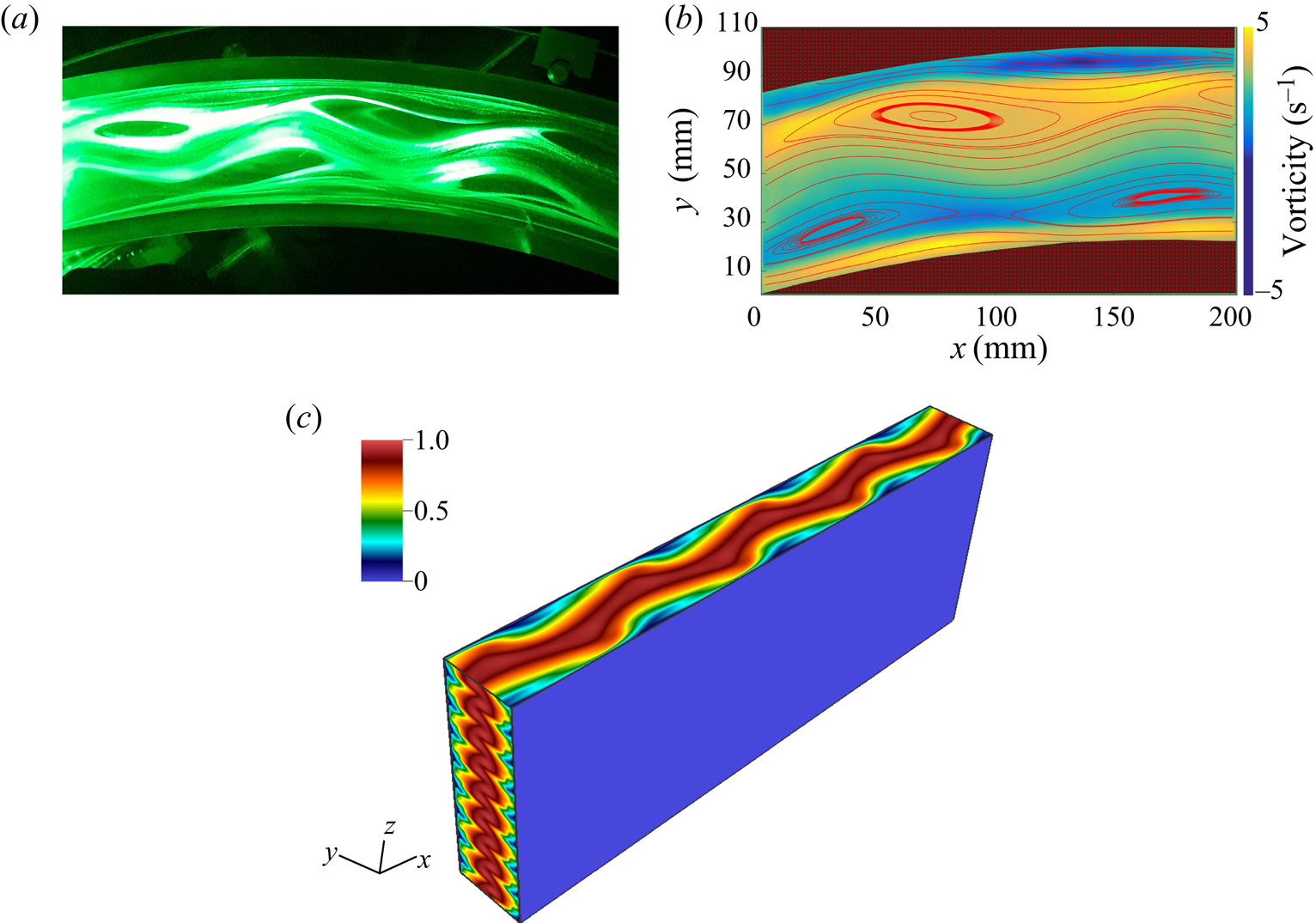
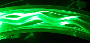
Visualizations and PIV measurements show the appearance of a nearly stationary pattern relative to the laboratory (in some cases a small drift is detected) composed of interfering oblique waves. It appears only above a threshold depending on the Reynolds numbers $Re$ and on the Froude number $F$. Figures 3(a) and 3(b) present a laser plane kalliroscope visualization (adding reflective platelets in water) and PIV measurements of the instability that takes the form of meanders in horizontal planes. These meandering flows are confined in thin layers along the vertical direction and have a strong visual similarity with the patterns of the unstable 2-D Poiseuille flow recently discovered by Falkovich & Vladimirova (Reference Falkovich and Vladimirova2018). We also show in figure 3(c) the numerical results for similar parameters, $Re=2800$ and $Fr=0.7$, but in a periodic channel. The results are shown for the end of the exponential growth phase when the linear instability saturates. We observe the same meandering, despite the differences between the experiments and the idealized periodic simulations.

Figure 3.

(a) Kalliroscope visualization of the meandering and recirculation eddies in a horizontal plane (adding reflective platelets in water). (b) An example of PIV measurements of the velocity field shown here by its streamlines and associated vertical vorticity field in background colours; here $F= 0.70$ and $Re= 2866$. (c) Velocity amplitude from DNS for $Re=2800$, $Fr=0.7$ and $Sc=7$ in a periodic channel. Results are shown during the early stages of the nonlinear saturation.

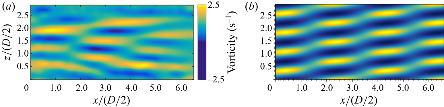
We have also realized experimental visualizations and velocity measurements in the median vertical plane located at $y=0$ and neglecting the curvature of the channel. Figure 4(a) shows an example of our PIV measurements that illustrates the layered pattern, similar to that already observed in plane Couette flow by Facchini et al. (Reference Facchini, Favier, Le Gal, Wang and Le Bars2018). Therefore, as can be observed on horizontal and vertical plane velocity measurements, the periodic arrangement of the meanders in horizontal planes is in phase opposition with each of its neighbouring layers. Note also the difference between the horizontal scale of the pattern, which is about 10 times larger than the thickness of each layer. This typical feature is again qualitatively confirmed by the periodic DNS, for which a very similar pattern is observed during the linear phase (see figure 4b).

Figure 4.

Observation of the horizontal vorticity field in the vertical plane showing the layered structure reminiscent of wave interaction. (a) Experiment with $F= 0.67$ and $Re= 2741$. (b) DNS with $Fr=0.7$, $Re=2800$ and $Sc=7$ in a periodic channel. Results are shown during the linear phase of the instability. The same window as (a) is shown in dimensionless units.

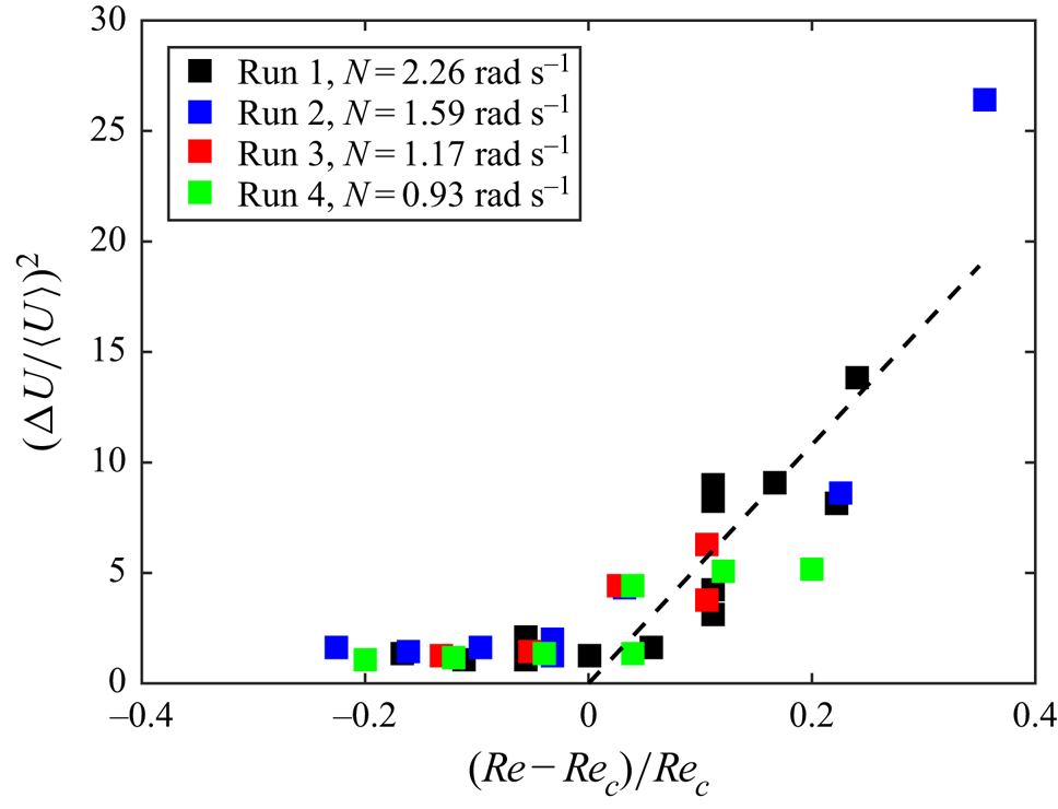
By repeating the experiment for different Reynolds and Froude numbers, it is possible to measure the sensitivity of the instability threshold on these parameters and to compare it with the theoretical predictions presented in § 5. Moreover, using these threshold values, we can plot in figure 5 the bifurcation diagram of the instability, gathering all our measurements by calculating a reduced Reynolds number $(Re-Re_c)/Re_c$. We found that the best way to represent the evolution of the instability finite amplitude is to compute, from the time-averaged PIV fields, the value ${\rm \Delta} U = U_{max} - U_{min}$ (which eliminates the base flow) divided by $\langle U\rangle = (U_{max} + U_{min})/2$, where $U_{max}$ and $U_{min}$ are the minimum and maximum of the horizontal velocity in vertical planes. The average being taken on a 4 s temporal window, the scatter of the data points comes from some fluctuations of the amplitude of the velocity fields measured at different times during each run. Despite this relative non-stationarity of the flow, the bifurcation seems to be supercritical, with a classical exponent $1/2$, as can be seen from the linear fit.

Figure 5.

Supercritical bifurcation of stratified Poiseuille flow. The dashed line on the right part of the graph is calculated from a linear fit of the whole set of measurements. Each critical Reynolds number has been first obtained by interpolation between the stable and unstable data.

5. Linear analysis of the instability

In this section, the main results obtained by the linear stability analysis of stratified plane Poiseuille flow are summarized. A more complete account can be found in Chen (Reference Chen2016). To perform the stability analysis, we use a pseudo-spectral code (already used in Chen et al. (Reference Chen, Bai and Le Dizès2016)) that solves the linearized Boussinesq Navier–Stokes equations for the normal-mode perturbations. For given streamwise and transverse wavenumbers $k_x$ and $k_z$, and given base flow parameters $Re$, $Sc$ and $F$, the code provides the complex frequencies $\omega$ of the eigenmodes.

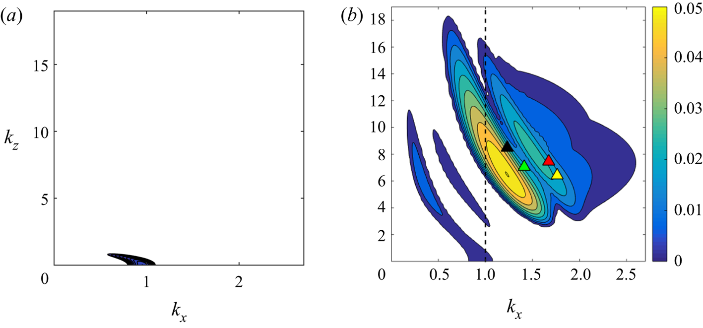
Typical stability diagrams with and without stratification are displayed in figure 6 for a stratified and a non-stratified base flow. We clearly see in this figure that the presence of stratification enhances the instability. For the non-stratified configuration (figure 6a), we observe a single instability mode that corresponds to a viscous TS wave. In the stratified case (figure 6b), this mode is still present and is unstable in a larger wavenumber domain. But the most striking feature of the stratified case is the presence of numerous other instability modes, which are more unstable than the TS wave. These modes have been generated by adding stratification. Note that we have run a DNS for the same parameters ($Re=10^4$, $F=1.1$ and $Sc=1$) and found perfect agreement on both the growth rate and the wavenumbers of the most unstable mode.

Figure 6.

Growth rate contours in the ($k_x, k_z$) plane for $Re = 10^4$ and $Sc=1$ and two values of the Froude number $F$: (a) $F=\infty$ (non-stratified case) and (b) $F=1.1$. Both plots use the same colour bar, with contours every $0.005$ from $0.001$ to $0.05$. Superimposed in panel (b) are the experimental data points coming from the four experimental runs: run 1 (black triangle), run 2 (green triangle), run 3 (yellow triangle) and run 4 (red triangle). The dashed line $k_x = 1$ represents the cross-section made for figure 7.

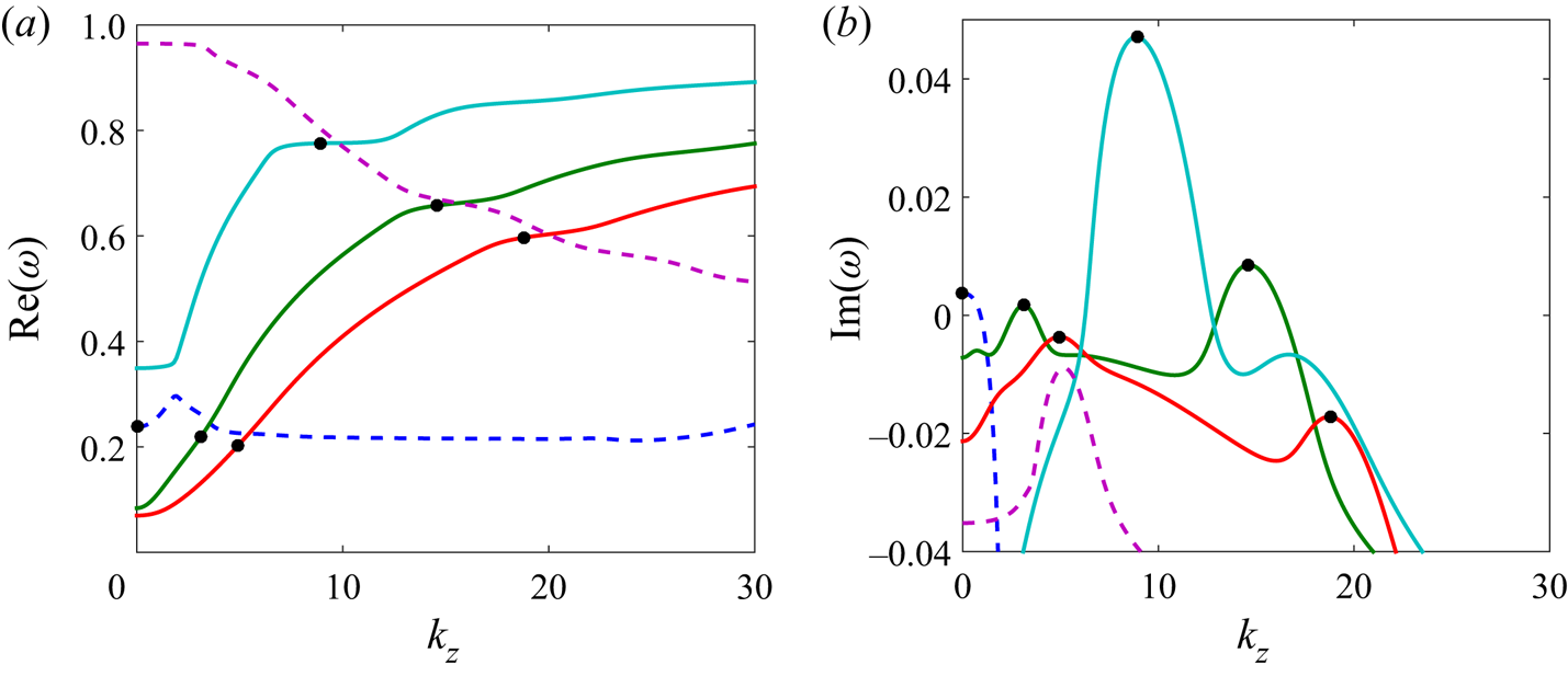
To understand the mechanism of instability, we plot in figure 7 both the real frequency $\textrm {Re}(\omega )$ and the growth rate $\textrm {Im}(\omega )$ of the different modes involved in the stability diagram of figure 6(b) as a function of $k_z$ for $k_x=1$. By this procedure, we can identify in the frequency plot (figure 7a) five different branches of modes involved in the instability diagram. By examining the shape of the eigenfunctions along the $y$ direction, it is possible to discriminate the origin of each of these modes (see Chen Reference Chen2016). The dashed curves are found to correspond to viscous TS waves, while the solid curves are associated with internal gravity waves. The black symbols indicate the points where the growth rate is locally maximum. We clearly see in figure 7(a) that these points are very close to the crossing points of the viscous and gravity wave frequency curves. The instability mechanism can thus be attributed to a phenomenon of resonance between viscous and gravity waves.

Figure 7.

(a) Dispersion relation of the waves calculated by following the eigenvalues of the linear stability analysis of the flow for $Re= 10^4$, $F= 1.1$ and $k_x=1$. As can be noticed, some intersections of these dispersion relations are possible. (b) Growth rates of the instability corresponding to the aforementioned intersections of dispersion relations – resonance areas are visible. The dashed curves are the frequencies and growth rates of the viscous modes, whereas the other solid curves are the dispersion relation of inviscid gravity modes.

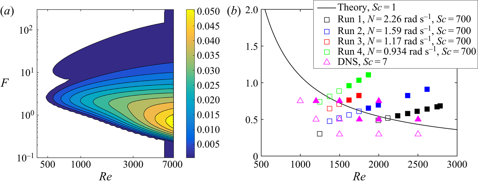
Such a resonant mechanism has been observed in other contexts (see e.g. Satomura Reference Satomura1981; Le Dizès & Riedinger Reference Le Dizès and Riedinger2010; Facchini et al. Reference Facchini, Favier, Le Gal, Wang and Le Bars2018) but it generally involves the coupling of inviscid waves only. The coupling with a viscous wave seems to be new, at least in the considered configuration with density gradients perpendicular to the plane of shear. For a fixed Schmidt number, the maximum growth rate of all the unstable modes can be calculated as functions of the Reynolds and Froude numbers. The results are summarized in figure 8(a) for $Sc=1$. The growth rate contours are shown for the intervals $400 < Re < 7000$ and $0.1 < F < 300$ in the ($Re, F$) plane. The critical Reynolds number is found to be $Re_c\approx 480$ for $F_c\approx 2.6$, well below the critical Reynolds number $Re_{TS}\approx 5770$ of 2-D TS waves. For moderate Reynolds numbers, we observe a large band of unstable Froude numbers. For instance, for $Re = 5000$, the instability extends from $F \approx 0.259$ to $F \approx 256$, with an extremum at $F\approx 0.8$.

Figure 8.

(a) Contours of the maximum growth rate in the $(Re, F)$ plane. Contours are every 0.005 from 0.001 to 0.05. (b) Comparison between the instability thresholds observed in the experimental runs for $Sc= 700$ (squares) and in the DNS for $Sc=7$ (magenta triangles). Open symbols correspond to stable configurations while solid symbols correspond to unstable cases. The theoretical curve for $Sc=1$ is shown as the solid black line.

6. Comparison with the experimental and numerical results and discussion

The wavenumbers $k_x$ and $k_z$ can be estimated from the PIV measurements. These values are reported on figure 6(b) presenting the predicted instability regions obtained from the linear stability analysis. Note that the vertical wavelengths have, as expected, the order of magnitude of the buoyancy scale $\lambda$ (Billant & Chomaz Reference Billant and Chomaz2001), which in our notation is equal to $FD$. For an average Froude number $F \approx 0.7$ as realized in our experiments, $\lambda$ is about $3$ cm, which in agreement with figure 4.

Similarly, we have plotted in figure 8(b) the experimental data and the marginal stability curve calculated from the theory at $Sc=1$. Interestingly, we observe a good agreement for the threshold values even if the Schmidt numbers for the theoretical analysis and for the experiments are quite different: in fact, we could have expected a lower experimental threshold because of the high value of the salt-water Schmidt number. Even if this were not the case, the observed agreement is a good indication that the instability is indeed associated with the mechanism of resonance that we have identified.

To explore the stability diagram further, we have also run DNS with parameters comparable to those of the experiments but in a doubly periodic channel and with a Schmidt number of $Sc=7$. All unstable experimental cases are also found to be unstable numerically. However, as can be seen in figure 8(b), some cases considered stable in the experiment and in the theory are found to be unstable numerically. This discrepancy could be attributed first to the already evoked differences in Schmidt numbers: $Sc=1$ for the linear stability analysis, while $Sc=7$ in the DNS and $Sc=700$ in the experiments. More likely, and even if the effects of rotation and curvature can be discarded because of the quite large values of the Rossby number, we can notice that the experimental base flow is slightly different than the 2-D planar parabolic Poiseuille profile (see figure 2) used in the theory and in the DNS. This small departure could indeed affect the stability threshold of the flow. Finally, we can also evoke the amplitude sensitivity of the measurements. As in any experimental instability study, the unstable flow needs to reach finite-amplitude saturated states before being detectable. Moreover, close to threshold, these nonlinear regimes need a very long time to establish and our observations may have missed them.

To conclude this discussion, we think that a combination of these different reasons is probably responsible for the observed and unexpected delay of the instability threshold observed experimentally, but this should not underplay the otherwise good qualitative agreement between all of our three approaches.