The boll weevil is enshrined in song, folklore, and many popular accounts as America's most destructive agricultural pest. Testifying before Congress in 1903, the chief of the Bureau of Plant Industry at the U.S. Department of Agriculture (USDA) referred to the insect's advance as “the wave of evil.”Footnote 1 In his annual address to Congress in 1905, President Theodore Roosevelt informed anxious cotton producers that USDA scientists had imported a predatory ant from Guatemala that fed on the weevil.Footnote 2 The weevil was indeed a headline grabber. Alas, the USDA's biological warfare program failed when the weevil-killing ant proved to be a humbug.
Social scientists offer two competing accounts of the weevil's impact on the economic development of the American South. Many scholars view the arrival of the boll weevil in 1892 as a revolutionary, negative productivity shock in a poor, cotton-dependent region. In One Kind of Freedom, Roger Ransom and Richard Sutch wrote: “It required a shock nearly equal to emancipation to jolt the agrarian South out of the routine it followed for the four post-emancipation decades. That shock was the coming of the boll weevil.”Footnote 3 James Street termed the weevil's invasion a “disastrous experience.”Footnote 4 Carolyn Merchant argued that the arrival of the boll weevil reduced “cotton yields by about 50 percent … the entire economy of the South was at risk.”Footnote 5 The arrival of the pest is commonly seen as one of the triggers of the “Great Migration” of African Americans to the North after 1915.Footnote 6
A range of scholars including James Giesen, Douglas Helms, Robert Higgs, Kent Osband, and Gavin Wright have argued that such accounts seriously exaggerate the insect's impact on the southern cotton industry specifically and on southern society as a whole. Their fundamental point is that, due to conditions in world cotton markets, the reductions in supply caused by the weevil led to offsetting increases in prices. In Old South, New South, Wright asserted that given the elasticity of demand for cotton, “the South as a whole did not suffer as a result of the boll weevil… . Each new attack simply caused the price received by all the other areas to be raised, thus serving, if anything, to keep cotton culture strong in older areas of the East longer than it otherwise would have been.” While the weevil did have “a lasting effect on cultivation practices … most parts of the South worked it into their routine and returned to ‘normal.’ What it did not do was to trigger a major diversification of southern agriculture or a new shift of resources out of agriculture into industry or other pursuits.”Footnote 7 Higgs concluded that “the boll weevil infestation was neither a necessary nor a sufficient condition underlying the Great Migration.”Footnote 8 And as Giesen observed, the South produced more cotton in 1921 than in 1892.Footnote 9
Thus a divide exists between the early accounts emphasizing the destructive impact of the weevil and the later general equilibrium analysis arguing that the response of cotton prices shielded the American South from this negative productivity shock. This divide can be bridged by realizing that even though the cotton industry as a whole expanded during this period, the weevil did in fact inflict serious and lasting damage on local economies. Due to a lack of sufficiently disaggregated data, research to date has focused on the effect of the weevil at the state level or on the South as a whole. We have assembled new data sets with county-level information on the production of both cotton and corn (the main alternative crop), total land use, land values, and population movements. With these new data sets, we can investigate how the spread of the weevil affected local economies and provide sharper estimates of the overall impacts and their timing relative to the date of first contact. We show that as the weevil traversed the American South, it seriously disrupted local economies, significantly reduced the value of land (at this time still the most important asset in the American South), and triggered substantial intraregional population movements. Our analysis reveals that the local impact of the weevil was devastating, even though the overall cotton economy expanded as suggested in the revisionist literature.
The article begins by documenting the coming of the boll weevil and describing its life cycle, migration patterns, and means of damaging cotton. The next section discusses the few techniques available to farmers to combat the pest. The third section explores the existing literature on the costs imposed by the weevil. Section four describes our two new county-level panel data sets, and section five presents our analysis of the boll weevil's impacts on agricultural production in local areas. The final section investigates the pest's impacts on land values and population.
THE COMING OF THE BOLL WEEVIL
The boll weevil, Anthonomus grandis Boheman, is a small beetle––about 1/4 inch long––with wings and a very pronounced snout.Footnote 10 Native to Mexico and Central America, the weevil was thought to have entered the United States in 1892 near Brownsville, Texas and thereafter advanced 40 to 160 miles a year (see Figure 1). By 1922 it had swept up the Atlantic seaboard and infested virtually the entire Cotton Belt.
USDA MAP OF THE SPREAD OF THE BOLL WEEVIL, 1892–1922

In the American South, boll weevils fed almost exclusively on the cotton plant. Cotton was planted in March and April and six to eight weeks later developed squares (flower buds). Early in the season, weevils fed on the leaves, before moving to the squares and bolls. The weevils continued to feed until the cotton plant was destroyed or killed by frost. Adult weevils punctured the squares to lay their eggs, typically depositing one egg to a square. Larvae, pupae, and adults would feed and develop inside the protective squares, until the insects' activity caused the squares to shed and release the new adults. With each female producing 100 to 300 eggs per generation for up to eight generations per year, the weevil population multiplied quickly as the season progressed. One consequence of this buildup was that late-season crops suffered the greatest losses. Warm, wet, cloudy summers were conducive to the heavy infestations, whereas very hot, dry summers killed larvae and pupae in the squares and young bolls, thereby limiting crop damage.
Adult weevils survived the winter without food by going into hibernation. Cold weather and standing water could kill the overwintering adults, but yard and field trash, nearby woods, and Spanish moss provided protection. Many of the control efforts were devoted to denying the weevil a safe place to survive the winter. Weevils that did survive emerged during the warm days from March until July. Even a small number of survivors could cause serious problems as one pair of weevils could generate millions of progeny in a single season.Footnote 11 In August, weevils entered a period of seasonal migration during which they could travel one hundred miles, typically following the prevailing winds. Weather events such as the great Galveston hurricane of September 1900 carried boll weevils far beyond their existing range.
Farmers and local authorities could do little to prevent the boll weevil from entering their territory, implying that the timing of arrival was largely exogenous. Once the insect hit, it was occasionally driven out by unfavorable weather and was subject to limited control by the cultivation practices discussed later.Footnote 12 First contact usually occurred during the August seasonal migration, too late to build up significant populations or do much damage in that year. Maximum damage occurred after the local weevil population became established and multiplied. Thus, the classic USDA maps detailing the spread of the weevil present a somewhat misleading picture of the area ravaged by the insect.Footnote 13 Such maps also create inaccurate impressions because many counties initially invaded, for example in southern Texas, were not producing much cotton. This was also true for many counties on the fringes of the Cotton Belt shown as weevil-free.
THE SPREAD OF THE BOLL WEEVIL AS A PERCENTAGE OF TERRITORY, COTTON ACREAGE, AND PRODUCTION WITHIN THE COTTON BELT, 1892–1922
To put these issues into context, we have compiled data showing when the weevil invaded each county in the Cotton Belt, and then weighted each county by its cotton acreage and production, as reported to the 1889 Census.Footnote 14Figure 2 plots the weevil's spread as a percentage of the Cotton Belt's cotton acreage and cotton production. The figure also shows the land area infested—the usual measure of the boll weevil's progress. All three series provide a sense of the timing of the pest's spread. The production-weighted series shows a relatively slow advance until 1897 and then an acceleration in diffusion over the 1898–1905 period. This was the period when the insect's path of destruction made its eastward turn. By 1907 the weevil had crossed the Mississippi River. In 1909 the production- and acreage-weighted series cross and after that date the traditional land-area measure understates the insect's probable impact as it advanced along a fairly regular front from west to east. In 1915, for example, the production-weighted series is 7 percentage points above the traditional land-area measure. By 1921/22 the insect completed its geographical conquest of the Cotton Belt.
CONTROL METHODS
From 1894 onwards the USDA, various state agencies, private companies, amateur scientists, farmers, and numerous quacks sought ways to limit the insect's damage. Insecticides proved ineffective. Efforts to erect quarantine buffers also came to naught. An early proposal in Texas to establish a 50-mile wide cotton-free zone ran into legislative resistance.Footnote 15 By 1904, when Georgia adopted quarantine measures, the weevil was too well established to be stopped. Many ideas on how to coexist with the weevil diffused rapidly. Entomologists recommended early maturing varieties, fertilizers to hasten ripening, early planting, more thorough cultivation, destroying stalks and brush, and locating fields away from woods and other places that harbored the pest.Footnote 16
It did not take farmers long to switch to earlier maturing varieties. The boll weevil entered Robertson County, Texas between 1898 and 1901. By 1901 farmers in that county were importing seed from northern Texas, and by early 1904 the Dallas Jobbers' Cotton Association had imported 19 carloads of seed from North Carolina. According to Helms, “One estimate held that Texas farmers imported thousands of car loads of short staple cotton seed in the rush to adjust to weevil destruction.” As the weevil spread, so did the transition in varieties, with some farmers, such as those in the Yazoo-Mississippi Delta, apparently switching in advance of the destruction.Footnote 17 In addition to adopting earlier ripening varieties, farmers sought other means to promote earlier crop development, such as moving up the planting dates by several weeks.Footnote 18Figure 3 offers a quantitative indication of the movement to earlier ripening varieties and associated cultural changes by charting the dates of cotton ginning. In the 1902–1907 period, less than 45 percent of U.S. cotton was ginned before the 18th of October. By 1934–1939 almost 70 percent was ginned by that date.Footnote 19
PERCENTAGE OF SOUTHERN COTTON GINNED BY SELECTED DATES, 1902–1940
For over a century, southern plant breeders had selected and acclimated cottons for specific areas. The boll weevil caused movement away from later-maturing, longer-staple varieties, rendering much of this investment obsolete. Characteristics such as fiber quality, picking ease, and storm resistance lost importance in the face of one overriding concern—early maturation. Picking efficiency and quality suffered as growers abandoned 1 1/8th inch “Big Boll” cotton for varieties with small bolls and very short (5/8th inch) staples. Roughly 50 long-staple varieties of cotton (as well as a number of high-quality mid-staple varieties) ceased to be commercially viable and eventually became extinct.Footnote 20
Cotton scientists found that burning or plowing under the cotton stalks immediately after the harvest reduced the number of weevils before they hibernated and significantly reduced the next year's damage. But according to Helm's careful investigation of this issue, the practice was not widely adopted, not only because it required much additional labor, but also because farmers would not capture the full social benefit of their labor. The weevils could migrate to nearby fields, meaning that an individual farmer would not be fully protected unless his neighbors followed suit. Success required a community effort. USDA scientists understood this externality problem and in 1896 unsuccessfully urged Texas state officials to enact legislation to establish mandatory stalk destruction dates.Footnote 21
Effective poisons, which would eventually become the key line of defense, were not available during the first wave of destruction. This was not for want of trying, as both farmers and entomologists experimented with the insecticides, including arsenic sprays and powders, that had been used against other pests. But the weevil grubs feeding inside the squares were well protected from toxins, and the cotton plant's foliage gave the adults considerable shelter from contact poisons. The first effective poison—a calcium arsenate mixture for dusting—was developed in 1918 by the USDA's B. R. Coad. The calcium helped the insecticide adhere to the plant, making it more accessible to the weevils. The discovery of an effective poison was only part of the story because application methods also had to be perfected. After numerous experiments, the USDA recommended that farmers raise a large dust cloud at night or in the early morning and let it settle while dew was still on the plants. In addition, there were trials with dusting machinery ranging from hand dusters, to mule and tractor towed devices, to airplanes. Calcium arsenate was costly and beyond the reach of many farmers.Footnote 22 In the period under consideration, farmers had limited ability to combat the bug, besides shifting to lower-yielding, earlier-maturing varieties or curtailing cotton production.
ECONOMIC IMPACTS OF THE BOLL WEEVIL
There is considerable controversy about the economic magnitude of boll weevil damage. The conventional opinion is that the weevil devastated production in the affected areas, but that the detrimental impact on production was relatively short-lived. A typical view is that the weevil destroyed “between one-third and one-half of the crop in newly infested areas.”Footnote 23 A number of studies reported large losses due
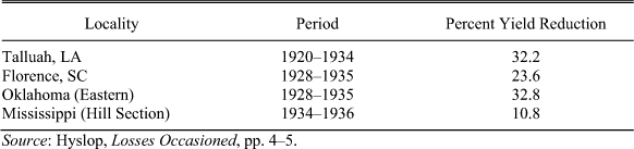
BUREAU OF ENTOMOLOGY AND PLANT QUARANTINE ESTIMATES OF WEEVIL DAMAGE

Source:
Hyslop, Losses Occasioned, pp. 4–5.
to the arrival of the weevil. The Bureau of Agricultural Economics (BAE) began estimating annual boll weevil losses from full yield in 1909. Over the 1909 to 1940 period, the estimated reduction in yield for the United States (excluding the weevil-free Far West) ranged from a low of 1.3 percent in 1911 to a high of 31 percent in 1921 and averaged about 10.5 percent overall.Footnote 24
Researchers from the Bureau of Entomology and Plant Quarantine (BEPQ) arrived at substantially higher estimates. They conducted studies across the South that compared “the yield in plots where the boll weevil was controlled with that in untreated plots.”Footnote 25 The results, summarized in Table 1, suggest that average physical losses were in the range of 11 to 33 percent.
In One Kind of Freedom, Ransom and Sutch present even larger estimates of the short-run losses caused by the boll weevil. Using annual state-level data for Louisiana, Mississippi, Alabama, Georgia, and South Carolina, they compare average cotton acreage and yields for the four years before the weevil first entered each state with the four years after the weevil had completely crossed through. Adopting these wide time frames was necessary because damage increased for several years after contact as the weevil population built up. The weevil typically required about six years to cross a state, making the mid-points of the periods under comparison roughly a decade apart. These calculations reveal that the infestation reduced cotton acreage by an average of 27.4 percent and yields by 31.3 percent.Footnote 26
By way of contrast, Osband, one of Sutch's students, presents considerably smaller estimates of the financial (as opposed to crop) losses. Osband noted that for all the damage done when the weevil arrived in a particular locale, the Cotton South as a whole was resilient.
“Cotton farmers learned to cut their losses to the weevil: They changed their cultivation methods, harvested sooner, and applied poisons. After the initial shock, every state witnessed a decline in weevil losses and resurgence of cotton production…. Overall, the weevil seems a symbol less of King Cotton's collapse than of its perseverance.”Footnote 27
The key observation was that the demand for southern cotton was characterized by an elasticity close to unitary. As a result, weevil-induced reductions in cotton output led to almost exactly offsetting increases in prices. Osband estimated that the aggregate annual revenue loss to southern cotton producers was a modest 2 percent. From this perspective, the higher cotton prices greatly benefited foreign producers and hurt consumers everywhere. Even within the South, some producers initially benefited while others suffered. Osband argues that taking into account the elasticity of cotton demand, the micro-level evidence that “the weevil triggered a transition out of cotton” is consistent with macro-level evidence of little long-term impact.Footnote 28
Osband's argument is consistent with the finding that the weevil reduced yields and production over long periods of time. The observed production in an area might have recovered because high cotton prices led farmers to intensify their efforts. Yet, these same farmers would have produced even more cotton (of far higher quality) in the absence of the weevil. This distinction is crucial. To understand the role of the weevil on the American South, we require both estimates of the direct impact of the weevil as well as of the equilibrium response to increases in world prices as the weevil affected more and more of the South. Using USDA state-level production data, Osband argues that instead of falling, equilibrium production actually rose.
Osband's finding that changes in prices largely offset output losses for the South as a whole adds significantly to our understanding of the pest's impacts. But it reveals little about how the local economies within the region were affected by the arrival of the weevil, or how those economies recovered from this shock. Furthermore, regional-level analysis does not reveal how farmers adjusted either before or after the weevil's arrival, or how the weevil affected local-level migration patterns and land values. Price increases might have reduced the overall impact of the weevil on the prosperity of the cotton-growing region. However, most historical accounts suggest that the boll weevil hit local communities with the force of a tsunami, causing large and immediate changes in production relationships. Investigating how these local economies responded to such a massive adverse shock to the leading staple commodity will advance our understanding of the South's economic institutions and long-run performance.
TWO NEW DATA SETS
This study departs from previous research by assembling new county-level panel data sets to investigate the magnitude and timing of the effects of the boll weevil. A county-level approach avoids many of the aggregation problems plaguing state-level studies and increases by orders of magnitude the number of degrees of freedom in our econometric analysis. We utilize two new sets of data. The first—census data—exploits the Censuses of Agriculture for the years 1889, 1899, 1909, 1919, 1924, and 1929. This data set contains county-level data on cotton production and acreage and allows us to construct a measure of yields. This data set also includes county-level characteristics (such as population, land values, and geographic coordinates) from sources using U.S. Census Bureau statistics.
The second data set—ginning data—contains annual data on cotton ginned within each county from 1899 to 1932. These statistics are from a set of U.S. Department of Commerce surveys of local ginners.Footnote 29 While ginning is not a direct measure of local production, the ginning data correlates closely with the census production data. For example, the correlation coefficient across counties in the 1899 Census is 0.99. The ginning data do not allow us to calculate yields, but they have the great advantage of being available annually.Footnote 30
Both data sets employ the same timeline of the weevil's spread. Using the classic USDA boll weevil maps, we code the year the weevil first arrived in a county, the year it had passed completely through the county, as well as the years of its various retreats and returns. The frontier lines are drawn at the end of each crop year, after the weevil's period of seasonal migration. We use the average of the start and through years to indicate the weevil's presence in a county. To provide weather controls at the local level, we create selected temperature and precipitation variables from two historical climate data sets. Specifically, we construct variables for each county's mean temperature in January and its precipitation in May, June, and July using data from nearby weather stations.
To create our panels, it is necessary to address the fact that the boundaries of many southern counties (N = 138) changed over our sample period. We form multicounty aggregates (N = 44) to use in place of those counties with boundary changes. We use these multicounty aggregates together with the counties having consistent boundaries (N = 1,165 in the full data set).Footnote 31 We refer to both types of geographic units as counties.
SAMPLE SELECTION
We select the sample with the goal of creating balanced panels of uniform, consistently defined geographic units possessing continuous measures of activity (production and acreage in the census sample and ginning in the ginning sample) for the period 1889–1929. To analyze the data, we require a simple time pattern for the presence of the boll weevil, which leads us to drop those counties that were never hit or saw a temporary disappearance of the weevil. Most of these counties were located at the edge of the Cotton Belt. As many of our specifications have log production, log acres, or log yields as their dependent variables, we are wary of putting undue weight on very small producers. Consequently, we exclude counties with minimal initial cotton acreage or production and drop observations that have very small production in some years.
Census Data
The data set includes 808 geographical units that were hit by the weevil and possessed consistent boundaries. Across six census years, these provide 4,848 observations. We drop 97 counties where the weevil entered, retreated, and then reentered. We exclude 90 counties that farmed less than 100 acres of cotton or had missing information on cotton production in the 1889 Census (the last taken before the arrival of the weevil in the United States). Finally, we remove 17 counties with less than 20 acres (or missing acres) of cotton production in any census year. The resulting sample contains 3,624 observations from 604 geographic units (that is, a 75 percent retention rate).
Ginning Data
To examine the timing of the impact of the weevil, we use ginning data from 1899 to 1932 (10 years after the last county was hit by the boll weevil). We limit ourselves to the years 1899–1929 whenever we compare ginning and census data results. As with the census data, we initially have 808 geographic units, which provide a total of 27,472 observations for the 34 years between 1899 and 1932. We also exclude the 97 counties in which the weevil entered, withdrew, and then reentered. We eliminate 173 marginal counties by dropping those with less than 100 (or missing) cotton acres in 1889, as well as those that in any year lacked ginning data or ginned less than 20 bales. The adjusted ginning sample contains 538 counties and 18,294 observations (a 66 percent retention rate).
LOCAL IMPACTS OF THE BOLL WEEVIL ON AGRICULTURAL PRODUCTION
The newly assembled data provide the means not only to examine the general trends in agricultural production, but also to investigate the localized impact of the weevil on agricultural production. Using the local data on agricultural production and the arrival of the weevil, we investigate how the weevil affected local output of cotton and corn (the main alternative crop). We consider the overall impact of the boll weevil, how farming changed in anticipation of its arrival, and how the impact varied with time after contact.
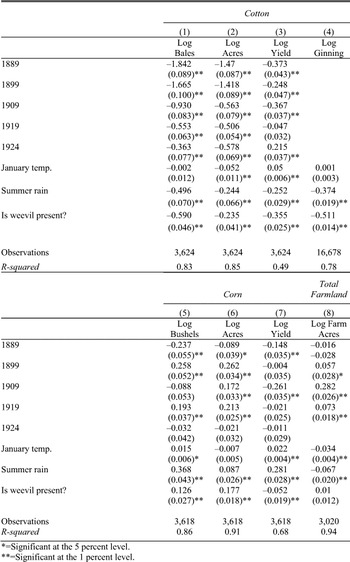
Our analysis shows consistently that the arrival of the boll weevil had large, persistent effects on local agricultural production activity in the American South. To provide a first look at the overall impact of the weevil on corn and cotton production, Table 2 reports results from a simple specification—a regression of various production measures on year and county fixed effects, local weather controls Wit as well as an indicator bwit for whether the weevil was present in county i at year t.Footnote 32 We also include a polynomial time trend interacted with the share of cotton sc in total acres harvested in 1889 to account for the growth in new cotton producers in this time period.

We initially focus on how the weevil affected cotton production. The first four columns of Table 2 show the results for cotton using both the census data (columns 1–3) and the annual ginning data (column 4).
The year dummies shown in the table for the census data and in Figure 4 for the annual ginning data inform us about the trends in cotton production common to all sample counties independent of the timing of contact. The top and bottom lines in the figure show the two standard error bounds. The data indicate a strongly negative general shock in 1921 relative to the surrounding years. Cotton production increased substantially during this period, especially rapidly between 1899 and 1909 and between 1924 and 1929. This confirms the macro-level findings of Giesen.Footnote 33
This secular trend toward increased cotton production contrasts sharply with the impact of the weevil on local production conditions. Our estimates from Table 2 suggest that the impact of the weevil on local production was huge. These county-level estimates imply that the weevil was associated with a decline in total output of about 50 percent. A comparison of columns 2 and 3 indicates that both yields and acreage declined, but that contact with the weevil led to greater yield losses than acreage reductions.
IMPACT OF THE BOLL WEEVIL ON AGRICULTURAL PRODUCTION


*=Significant at the 5 percent level.
**=Significant at the 1 percent level.
Notes:
Standard errors (in parentheses) are robust to heteroskedasticity (Huber-White). The variables 1889, 1899, 1909, 1919, and 1924 refer to year fixed effects; 1929 is the omitted year. Cotton: Columns 1–3 report estimates based on census data for 1889, 1899, 1909, 1919, 1924, and 1929. Column 4 reports estimates based on annual ginning from the commerce data 1899–1929. Corn and total farmland: Columns 5–8 are estimated on census data weighted by the share of cotton in total production in 1889. Currently no machine-readable data on total farmland in 1924 are available. All specifications with year and county fixed effects as well as polynomials in the fraction of farmland planted as cotton in 1889 interacted with a time trend.
Source:
See the text.
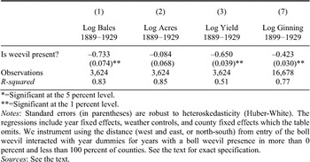
One might be concerned that our estimates may be contaminated by reverse causation: locally favorable production conditions for cotton are likely to have favored the weevil's spread. Mindful of this possibility, we instrument for the presence of the boll weevil using the geographic location of the county. In a given year, the distance of a county from Brownsville, Texas (the weevil's entry point) predicts extremely well whether the weevil was present in that county. The relationship between the county's distance from the point of entry and the indicator variable for the presence of the weevil obviously changed as the weevil advanced across the South, suggesting an instrumental variable strategy that exploits the geographic location of each county interacted with the year of measurement. Therefore our instruments consist of the distance in longitude east and west of Brownsville as well as the latitude of each county interacted with the years 1899, 1909, and 1919.Footnote 34 The exclusion restriction for this set of instruments is that production conditions did not change differentially with respect to latitude and longitude during the period 1899–1919. Table 3 displays the results for the second stage of the regressions on log bales, acres, yields, and ginning. The first-stage regression for presence of the boll weevil has an F-statistic (72 numerator dfs) of 101.76 for the ginning data and an F-statistic (9 numerator dfs) of 268.61 for the census data. We find that the estimated effect of the weevil on cotton production is stronger in the IV than the OLS regressions. Both our OLS and IV results are consistent with the literature that finds the weevil had a devastating local impact on cotton production. In fact, we find that the impact was even larger than the numbers traditionally asserted.
YEAR FIXED EFFECTS for cotton ginned, 1899–1929
The results in Tables 2 and 3 do not reveal how the impact of the weevil was distributed relative to the time of its arrival. Due to limitations arising from the use of state-level data, the existing literature contains only fragmentary evidence on this question. We observe local production measures over several decades. This allows us to determine much more precisely how the impact of the weevil was distributed relative to its arrival. We replace the variable for the boll weevil's presence with 10 leads and 10 lags for its arrival. The specification retains the local weather variables, the interaction of 1889 share of cotton in production with a time polynomial, as well as the county and year fixed effects.

IV-REGRESSION USING LONGITUDE AND LATITUDE

*=Significant at the 5 percent level.
**=Significant at the 1 percent level.
Notes:
Standard errors (in parentheses) are robust to heteroskedasticity (Huber-White). The regressions include year fixed effects, weather controls, and county fixed effects which the table omits. We instrument using the distance (west and east, or north-south) from entry of the boll weevil interacted with year dummies for years with a boll weevil presence in more than 0 percent and less than 100 percent of counties. See the text for exact specification.
Sources:
See the text.
In specification 2, hi represents the year that the weevil entered county i. We omit the indicator variable for the year that the weevil arrived in a county and thus measure all effects relative to its arrival. The years 10 or more after being hit are combined into a single categorical variable as are the years 10 or more before being hit.
Figure 5 presents the coefficients on the timing variable for log bales, yields, acreage, and ginning.Footnote 35 The graphs show the main effects as well as two standard error bounds. These production graphs put the destructive impact of the weevil into sharp relief. For instance, ginning fell by about 10 percent in the year after first contact and by more than 50 percent within the first five years of the arrival of the weevil. There is no sign that local activity rebounded within a decade of being hit. It is possible, indeed likely, that without the mitigating efforts of farmers, the local impact of the weevil would have been even greater.
The coefficient estimates for the pre-contact period inform us about how farmers behaved in anticipation of the arrival of the weevil. One might expect that as the weevil approached a given locality its farmers would lessen their dependence on cotton in order to reduce their exposure to the impending threat. But our results show that in the year of contact, more land was put into cotton, and more cotton was harvested and ginned, than two or three years before contact. The magnitude of the effect is statistically significant and economically large. For instance, at least 10 percent more cotton was ginned in the year of contact than in any of the preceding or following years.
PRODUCTION MEASURES RELATIVE TO THE ARRIVAL OF THE WEEVIL
Several explanations are possible. One is that this relationship is not the product of human intention. For example, good cotton-growing weather covering a large region might encourage both a big crop and a large population of exceptionally fast migrating weevils. (Poor cotton-growing weather might lead both to a bad crop and a delay in being hit, which could account for the dip in the years immediately before contact.) The regressions include partial controls for local weather with variables for January temperature and summer rain, but there may remain some omitted variable bias.
A second, more intriguing alternative is that the rise in production immediately before contact was a conscious human choice. Helms observed that “farmers too often attempted to grow that last ‘big crop’ after the boll weevil arrived.”Footnote 36 However, it might have been economically rational to seek to depreciate rapidly cotton-specific assets (equipment and soils) before the insect's attack lowered their productivity. The increase in production might also have been a response to enlarged local labor pools swollen by cotton hands moving east to escape the wave of destruction.Footnote 37
We attempt to distinguish between reverse causality and purposeful human behavior by instrumenting for the arrival of the boll weevil. Technically, specification 2 contains 20 endogenous variables, one for each dummy describing the time difference from the arrival of the weevil. However, that time difference is generated by only one variable: the actual arrival date of the boll weevil, and thus there is only one source of endogeneity here. To make progress, we estimate an ordered logit regression predicting the probability that the boll weevil will arrive in a county in a given year based on a flexible functional form measuring the distance from the weevil's initial point of entry into the United States.Footnote 38 Using this estimated probability of arrival, we can generate for each year and county a vector of probabilities measuring the probability that the weevil will arrive within k years. The variation in this probability, which is orthogonal to the included independent variables in specification 2, is generated by the distance of the county from the weevil's initial point of entry. We use this vector of probabilities of local arrival as an instrument for the timing variables. Figure 6 contrasts the OLS estimates on timing from the ginning data with the IV estimates.
The instrumental variable estimates of the timing pattern in Figure 6 do show the same general patterns as the OLS estimates. Both the OLS and the IV results show that the amount of cotton ginned declined rapidly after the weevil arrived. The estimates obtained from the IV procedure also confirm that ginning increased as the weevil approached. This suggests that the run up before the weevil's arrival was at least partially generated by human behavior and not due to reverse causality. However, the estimates from the IV are noisy and should be interpreted with caution. Implementing the IV procedure for timing with the census data proves a fruitless exercise because of noise.
GINNING RELATIVE TO THE ARRIVAL OF THE WEEVIL – OLS AND IV ESTIMATES
We also explore the possibility that the impact of the weevil differed across counties depending on the prior intensity of cotton production. To measure the cotton intensity of a county, we calculate the ratio of cotton acres to total farm acres in 1889 (the last census information before the weevil arrived in the United States). Figure 7 illustrates the distribution of this measure of the intensity of cotton (sc). It shows that most counties had less than 25 percent of their farmland in cotton production and only a few devoted more than 30 percent of land to the crop. We have already employed the variable sc in specifications 1 and 2 by interacting it with time polynomials. Here we investigate the interaction of this measure of cotton-production intensity with our main variable of interest: the presence of the weevil.
DISTRIBUTION OF COUNTIES BY COTTON INTENSITY
We augment specification 1 with a 4th-order polynomial of sc interacted with the variable indicating the presence of the weevil. This allows us to predict the impact of the weevil by the cotton intensity of counties. Figure 8 shows how the predicted impact of the weevil varies across the cotton intensity of the counties for our production measures. Panels A, B, and D indicate that the impacts on total production and on acres increased with a county's cotton intensity.Footnote 39 The bales produced (panel A) fell sharply as the cotton intensity rose from 0 to 10 percent of farm acreage—at the 10 percent intensity level, locations hit by the weevil produced about 55 percent fewer bales than those untouched. The relationship between cotton acres and intensity (panel B) follows a roughly similar pattern. Panel C shows that the presence of the weevil reduced yields by roughly 30 percent for all intensity levels. The ginning results (panel D) show a large negative impact even for locations with relatively little cotton. The weevil's negative impact continued to increase as the intensity of cotton production rose above 20 percent.
IMPACT OF THE BOLL WEEVIL ON COTTON PRODUCTION BY INTENSITY OF COTTON FARMING IN 1889
SUMMARY OF COTTON PRODUCTION RESULTS
The estimates from both the census and ginning data provide a consistent picture of the devastation the arrival of the boll weevil visited on local cotton production. Within five years of contact, total cotton production declined by about 50 percent. This decline, relative to unaffected counties, was permanent and evident in both cotton acreage and yields. The negative effects on yields appear to outweigh those on acreage. The weevil impacted most severely counties that were heavily concentrated in cotton in 1889. This may have reduced the economic position of cotton-intensive counties relative to counties that were only small producers before the arrival of the weevil. While the arrival of the weevil was locally devastating, its spread occurred during a period when overall cotton production in the South increased tremendously. Growth was especially rapid from 1900 to 1909 and 1924 to 1929 and was associated with increases in acreage (rather than yields).
ALTERNATIVE LAND USES RELATIVE TO THE ARRIVAL OF THE WEEVIL
TOTAL CORN BUSHELS, YIELDS, AND ACREAGE
The decline in cotton acreage raises the question of what southern farmers did with the released land. Some have argued that instead of shifting land to alternative crops, southern farmers simply abandoned cultivation.Footnote 40Table 2, as well as Figure 9 panels A and B, show that this
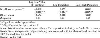
LAND VALUES AND POPULATION

*=Significant at the 5 percent level.
**=Significant at the 1 percent level.
Notes:
Robust standard errors in parentheses. The regressions include year fixed effects, county fixed effects, and quadratic polynomials in years interacted with the share of land in cotton in 1889 (omitted from the table).
Source:
See the text.
was not the case. Total farmland (column 8 and panel A) barely budged as the weevil moved through a county. Instead, southern farmers increasingly shifted production to the main alternative crop, corn. As seen in panel B, the acreage of land devoted to corn production increased by about 20 percent subsequent to the arrival of the weevil. Our estimates of the impact of the weevil on corn production and yields are noisy, but do nevertheless display some interesting patterns. Panel C shows that total production of corn increased by only 10 percent, even though land allocated to corn rose by about twice that amount. Corn yields declined subsequent to the arrival of the weevil, possibly because farmers differentially shifted less fertile land to its cultivation. Overall, the corn results indicate a greater movement to alternative crops than suggested in the literature, which has downplayed the boll weevil's effects on diversification.Footnote 41
LOCAL IMPACTS ON LAND VALUES AND POPULATION
We now investigate the local impact of the weevil's arrival on land values and population movements. The evidence in Table 4 indicates that real land values per acre declined on average by about 10 percent after contact. Perhaps more surprising, local populations appear to have increased with the arrival of the weevil.
The results presented in column 1 of Table 4 obscure interesting variations in the responses of land values. These responses differed over time and across counties depending on the importance of cotton in the local economy. Indeed, well-functioning real estate markets should have capitalized the pest's impact into land values long before it arrived in a given county. Thus, we need to consider how land values evolved prior to and following the weevil's arrival.
TIME VARIATION IN LAND PRICES
We enrich specification 2 to allow the effect of the weevil on land values to vary with the share of cotton in local agricultural production in 1889. That is, we interact a polynomial in the share of cotton in total acreage with the duration of time before and after the arrival of the boll weevil. This allows the estimation of the differential effect of the weevil on land values by share of production. The lines in Figure 10 graph how local land values varied in the 10 years before and after the weevil arrived in a county relative to the land value in the year of arrival. The start and end values of the lines represent the long-run averages of the more than 10 years before and after the weevil arrived. In each panel, we show the effect on land values for counties that differ in their intensity of cotton farming in 1889. We choose four intensity levels that capture most of the support of the distribution of cotton intensity.
As expected, the measured impact of the arrival of the weevil on land values depended on how much land was employed in farming cotton and varied with time relative to initial contact. In addition, we find important interactions between time and the dependency on cotton. Counties that were heavily engaged in cotton farming (shares 0.18 and 0.27) saw dramatic long-run declines in land values of around 20–40 percent in the 10 years prior and subsequent to the arrival of the weevil. Furthermore, these declines commenced long before the weevil arrived in a location. The arrival of the weevil and its effect on the productivity of land were well known, and the real estate markets of the South succeeded, at least partially, in pricing this into local farmland values prior to contact. However, for counties that were heavily engaged in cotton farming, land values continued to decline until about five years after the weevil arrived, mirroring the declines in productivity displayed in Figures 5 and 6.
The top two panels in Figure 10 display the impact of the arrival of the weevil on land prices in counties that were less dependent on cotton. Land values increased modestly in the five years prior to contact with a positive blip at about the time the weevil entered the county. From this peak, land values fell sharply before leveling off about five years after the weevil first appeared. The bottom two panels show the impact in counties more dependent on cotton. Here there is a general decline before and after the pest's arrival, but again there is a small positive blip around the time of contact. There are several possible explanations for this run-up in land values about the time the weevil hit. Farmers might have been bidding for land suitable for other crops as cotton farming became less attractive. We do not have breakdowns of prices by prior use and therefore cannot investigate the time-patterns in land values in more detail.
An alternative explanation is that the approach of the weevil released labor from cotton farming and thus lowered local wages. This would benefit land owners engaged in activities other than cotton farming. If the approach of the weevil indeed released large numbers of laborers from cotton-intensive counties, then we would expect that the population would rise in neighboring counties that were not heavily engaged in cotton farming. Furthermore, we would expect that migrant workers might move in advance of the weevil, swelling populations in those counties heavily engaged in cotton farming but not yet hit by the weevil. That is, we would expect a peak in population numbers in the year the weevil arrived in a county when farmers hoped to harvest one last bumper crop. Figure 11 shows total population movements surrounding the arrival of the weevil and Figure 12 shows movements in the black population. The data are consistent with the idea that labor migrated in advance of the weevil. Population movements were the most pronounced among those counties that farmed little cotton and those heavily reliant on the crop.
TIME VARIATION IN LOG POPULATION
Everywhere, as the weevil approached, the total population numbers swelled. Counties that produced little or no cotton (such as those on the fringe of the Cotton Belt) experienced massive demographic shocks with population surges of about 50 percent above the pre-weevil counts. Even ten years after being deluged with refugees, these counties were still well above their pre-weevil population levels. In counties that were heavily devoted to cotton production (share = 0.27), there was also a rapid increase in population just prior to the arrival of the weevil. This was followed by an exodus that saw about 30 percent of the peak population leave after about five years. The movements of blacks roughly mirrored those of the total population. Although our data say nothing directly about interregional migration, it is likely that the demographic shocks that displaced so many people within the South contributed significantly to the Great Migration to the North.
TIME VARIATION IN LOG BLACK POPULATION
We can conclude with some certainty that as the weevil approached, land values in counties that specialized in cotton production declined dramatically. This decline in land values away from the trend was not reversed during the time for which we have data. Interestingly, the movements in land values (Figure 10) were consistent with the population numbers.
CONCLUSION
County-level data offer dramatic evidence on the impact of the spread of the boll weevil. Our focus on the local impacts of the weevil differs from much of the cliometrics literature, which has largely explored the global or Southern-wide effects of the boll weevil and consequently downplayed the pest's importance. Our findings may be summarized as follows: contact with the boll weevil had large, immediate, negative effects on local cotton production, acreage, and especially yields; these adverse effects grew in magnitude during the first five years after contact and persisted for a least a decade—there is no evidence of local recovery independent of changes in cotton-production conditions common to the entire South; the impacts on yields exceeded those on acreage, suggesting a decline in efficiency; and just before contact, southern farmers expanded cotton production—as if trying to squeeze out one last big crop rather than beginning to diversify away from their threatened staple.
Turning to the effects beyond cotton production, we find little land was completely removed from agricultural production after contact, instead acreage was shifted to corn and other crops; local real estate values declined both in anticipation and in the aftermath of the weevil's arrival, especially in areas heavily dependent on cotton; the weevil appears to have unleashed a wave of internal migration, leading to local population gains before contact and substantial losses after the onset of significant crop damage; and the effects on land values and population varied systematically with the county's pre-boll weevil dependence on cotton.
Our findings of large local effects of the weevil open up interesting possibilities for future research. The spread of this pest through a relatively poor region that was heavily dependent on cotton represents an exogenous productivity shock that can be used to identify the internal workings of the southern economy. Understanding the response of the farm tenancy system to this shock promises to shed light on long-standing questions regarding Southern economic institutions. Tracing the impacts on how the time of Southern children was allocated between work and school would also be informative.
In summary, we document that the march of the boll weevil had dramatic, persistent consequences for those cotton producers in its course. While it is true that cotton production in the American South in 1921 exceeded that in 1892, before the pest appeared, the cotton grown in 1921 was on average of lower quality. As the weevil advanced, it triggered massive local population and production changes in the years before and after its arrival. Studies of the twentieth-century South cannot ignore the dramatic impacts this pest had on those in its path.
Appendix: Data Description and Sources
Extent of Boll Weevil Infestation
The extent of boll weevil infestation was based on the 1922 map appearing in Hunter and Coad, Boll-Weevil Problem.
Ginning Data
Annual county-level data on cotton ginning are available beginning in 1899 from the U.S. Bureau of the Census, Quantity of Cotton Ginned in the United States and Cotton Production in the United States. The data, including both the upland and Sea Island crops (exclusive of linters), are in number of 500-pound equivalent bales. Local agents collected the data based on a comprehensive canvas of southern ginneries. County-level ginning is very closely correlated to county-level production; the R-squared equaled 0.99 in the 1899 Census data.
Production and Farm Characteristics
The U.S. Census of Agriculture collected data on acreage, production, and thus yields for cotton, corn, and other crops by county for 1889, 1899, 1909, 1919, 1924, and 1929. Census data are drawn from Michael R. Haines and the Inter-university Consortium for Political and Social Research, Historical, Demographic, Economic, and Social Data: The United States, 1790–2000. [Computer file] and U.S. Bureau of the Census, Fifteenth Census of the United States: 1930, Agriculture. Vol. 3, Pt. 2, The Southern States, Reports by States, with Statistics for Counties and a Summary for the United States. Value of land and buildings per acre, in whole dollars, for 1924 are from Thomas J. Pressley and William H. Scofield, Farm Real Estate Values in the United States, 1850–1959 [Computer file]. The plantation counties were defined in U.S. Bureau of the Census, Plantation Farming in the United States.
Weather
The weather data come from two sources: (a) United States Historical Climatology Network (USHCN), http://www.ncdc.noaa.gov/oa/climate/research/ushcn/ushcn.html; and (b) National Oceanic and Atmospheric Administration, Nineteenth-Century U.S. Climate Data Set Project (based primarily on records kept at U.S. forts), http://lwf.ncdc.noaa.gov/oa/climate/onlinedata/forts/forts.html. We merge these data sources to estimate the temperature and precipitation variables for each county.