1 Introduction
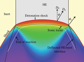
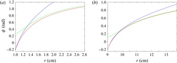
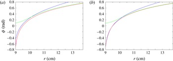
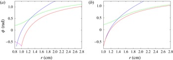
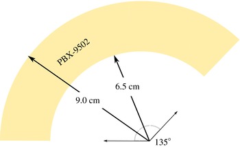
A detonation is a complex, compressible flow–reaction driven structure consisting of a lead shock wave and subsequent reaction zone in which reactants are converted into products. The volume expansion associated with the energy change due to reaction sustains the shock. For high-explosive (HE) applications, we need to be able to accurately describe the speed and path of a detonation as it moves through often complex three-dimensional (3D) geometries with various confinements. This then sets the stage for calculating how the energy released due to chemical reaction couples with the hydrodynamic flow to drive material surrounding the explosive. The speed of a one-dimensional detonation where the chemistry consists of a set of irreversible reactions is not influenced by the details of reaction zone structure, but is simply a function of the initial material state, the total energy release due to reaction and the equation of state of the products (Fickett & Davis Reference Fickett and Davis1979). In practice, the high pressure of the products results in yielding of any confinement at the explosive edges, and the detonation reaction zone structure becomes multi-dimensional and determined by a complex interaction between streamline divergence, compressibility and reaction (figure 1). In response, the detonation shock becomes curved. The structural details of this complex hydrodynamic interaction establishes the speed of the detonation as it sweeps through an explosive geometry. For quasi-steady or steady motion, only the reaction zone structure between the detonation shock and the flow sonic locus (in a frame travelling with the shock) determines the speed of the wave. For such flows, it is the influence of explosive geometry on the structure of this region that determines the speed of propagation of detonation and its time of arrival at a specific location in the geometry.
Despite the reaction zone complexity, the scale disparity between a typical reaction zone thickness and larger explosive geometry, which can be of the order of several hundreds or thousands, motivates a formal asymptotic analysis of the reaction zone structure under the limits of small detonation front curvature and slow time variation of the shape of the detonation front, relative to characteristic reaction zone length and time scales. Within the context of a hyperbolic compressible–reactive Euler model, such an analysis has been undertaken by Bdzil and Stewart (Bdzil & Stewart Reference Bdzil and Stewart1986, Reference Bdzil and Stewart1989; Stewart & Bdzil Reference Stewart, Bdzil, Buckmaster and Takeno1988a ,Reference Stewart and Bdzil b ; Bdzil, Fickett & Stewart Reference Bdzil, Fickett and Stewart1989). It was found that the detonation motion due to the reaction zone/detonation shock complex reduces formally to a surface evolution description where, to leading order, the normal velocity of the surface is a function of the local surface curvature. This asymptotically derived model is known as Detonation Shock Dynamics (DSD). By comparison with reactive flow model simulations or validation experiments, it has been shown that the DSD model can successfully capture the consequences of the complexity of the compressible–reactive flow interaction that determines the detonation speed for calculating detonation motion in complex explosive geometries (Bdzil et al. Reference Bdzil, Aslam, Henninger and Quirk2003; Lambert et al. Reference Lambert, Stewart, Yoo and Wescott2006; Hodgson Reference Hodgson2014; Jackson & Short Reference Jackson and Short2015). Recent reviews on the development and application of the DSD model are given by Bdzil & Stewart (Reference Bdzil and Stewart2007, Reference Bdzil, Stewart and Zhang2011). The effects of the impedance of the material surrounding the explosive (the confiner) on the timing are typically accounted for by specifying the angle of the surface at the HE/material interface, an issue on which we expand below. Level-set methods are commonly deployed in numerical calculations of the evolution of DSD surface motion (Aslam, Bdzil & Stewart Reference Aslam, Bdzil and Stewart1996; Hernández, Bdzil & Stewart Reference Hernández, Bdzil and Stewart2013; Meyer et al. Reference Meyer, Quirk, Short and Chiquete2016). Owing to its accuracy over traditional timing models that do not account for the influence of reaction zone flow structure on detonation speed, such as the Huygens model, the DSD model has become a mainstay for the detonation timing component of advanced programmed-burn models designed for explosive energy delivery calculations (Kapila, Bdzil & Stewart Reference Kapila, Bdzil and Stewart2006). This is especially the case for insensitive or non-ideal explosives where detonation front curvature can significantly influence the speed of the detonation motion.
A schematic of the induced detonation shock curvature and pressure variation through the detonation reaction zone for steady detonation propagation in a two-dimensional planar slab geometry due to lateral yielding of confinement. Higher-pressure regions are indicated by the red colouring, with lower pressure regions indicated by the blue colouring. The situation shown is for a case of weak confinement, where the sonic locus intersects the detonation shock at the HE/inert interface. The sonic locus lies ahead of the end of the reaction zone. Figure adapted from Bdzil et al. (Reference Bdzil, Aslam, Henninger and Quirk2003).

The surface evolution equation in the DSD model is of parabolic form (for non-zero curvature), derived as a submodel of the hyperbolic, compressible–reactive Euler model. Being parabolic, the model has no notion of supersonic, sonic or subsonic flow. Consequently, there are certain limitations of the DSD model. One such difficulty arises for the DSD model near the HE/confiner material interface where the details of flow characteristics in the hyperbolic model are important in defining the edge effects. In fact, the asymptotic assumptions underlying the DSD model can be shown to break down near the edge of an explosive (Bdzil Reference Bdzil1981). Consequently, in using the DSD model for engineering applications, the parabolic DSD model must be augmented with boundary conditions that, in some physically reasonable sense, mimic the HE detonation behaviour found in the hyperbolic, compressible–reactive Euler model near the edge of the explosive.
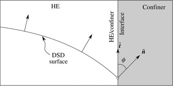
The procedure for deriving the DSD boundary conditions has been described in detail for three of the most common detonation wave/confiner interaction cases by Aslam et al. (Reference Aslam, Bdzil and Stewart1996), and reviewed in Bdzil & Stewart (Reference Bdzil and Stewart2007, Reference Bdzil, Stewart and Zhang2011). The motivation comes through an appeal to oblique shock polar theory applied locally at the HE/confiner interface. To model the situation of sonic or subsonic flow behind the detonation shock at the HE/confiner interface (in a reference frame moving with the velocity of the point of intersection of the local detonation shock and the confiner material boundary), an angle
 $(\unicode[STIX]{x1D719})$
between the normal to the DSD surface and the tangent to the material interface is imposed on the DSD surface at the HE/confiner interface (figure 2). The effects of supersonic flow behind the detonation shock at the HE/confiner interface for sufficiently oblique detonation waves is modelled by an extrapolation condition on the DSD surface shape. The angles that are used in the DSD model for the cases of sonic and subsonic flow can be obtained from the oblique shock polar analysis and relies on knowledge of the equations of state of the HE reactants and the confiner (Aslam & Bdzil Reference Aslam and Bdzil2002, Reference Aslam and Bdzil2006). A sonic flow angle
 $(\unicode[STIX]{x1D719}=\unicode[STIX]{x1D719}_{s})$
is imposed when the HE has no confinement, or is confined by a low-impedance material such as plastic. A subsonic flow edge angle (
 $\unicode[STIX]{x1D719}=\unicode[STIX]{x1D719}_{c}~({<}\unicode[STIX]{x1D719}_{s})$
) is imposed when the HE is confined by a high-impedance material such as copper or steel. In the DSD model described by Bdzil, Henninger & Walter (Reference Bdzil, Henninger and Walter2006), Bdzil et al. (Reference Bdzil, Aida, Henninger and Walter2007) and Hernández et al. (Reference Hernández, Bdzil and Stewart2013), the continuation condition used to mimic supersonic flow assumes that the DSD surface is locally straight, i.e. has zero curvature at the material boundary.
Schematic for the implementation of angle boundary conditions at the HE/confiner interface for the DSD model. Figure based on Aslam et al. (Reference Aslam, Bdzil and Stewart1996).

In the current paper, we are concerned with the construction of steady solutions for a DSD model of detonation propagation in a two-dimensional (2D) circular arc geometry. The arc is an important case for understanding the effects of geometry on the compressible–reactive flow mechanisms of detonation propagation in complex geometries, as it includes elements of shock diffraction, flow divergence (Bdzil et al.
Reference Bdzil, Fickett and Stewart1989) and a range of boundary interactions depending on the geometry (specifically the inner and outer arc radii), and the degree of confinement. This is the first paper in a two-part study, with the second focusing on reactive burn simulations of detonation propagation. The motivation for this second study was the surprising results obtained from the asymptotic analysis of the DSD model for thick arcs in the current paper, specifically the finding that a small boundary layer region along the inner arc surface is primarily responsible for the modifications to the speed of detonation propagation that occur due to the magnitude of the arc inner radius and the degree of confinement on the inner arc surface. Other studies of detonation propagation in an arc geometry have been conducted. Bdzil et al. (Reference Bdzil, Fickett and Stewart1989) examined detonation timing in several geometries using a DSD model, including one example of an arc geometry simulation where the arc was sufficiently wide to result in the need to use a surface continuation (supersonic flow-like) condition along the outer arc boundary. A DSD simulation of propagation in a 2D circular arc using a single surface evolution methodology was described in Bdzil et al. (Reference Bdzil, Henninger and Walter2006) for perfect confinement on the outer arc, and used as a verification solution for the full level-set-based DSD implementation described in Bdzil et al. (Reference Bdzil, Henninger and Walter2006, Reference Bdzil, Aida, Henninger and Walter2007). Aslam & Stewart (Reference Aslam and Stewart1999) compared the timing from a higher-order DSD model, which contained acceleration terms in addition to the usual curvature dependence, against the curvature-dependent DSD model in a 2D circular arc geometry, with perfect confinement on both inner and outer arc radii. Lieberthal, Bdzil & Stewart (Reference Lieberthal, Bdzil and Stewart2014) have also used a DSD model to study the response of a detonation shock wave passing over a periodic array of inert particles embedded in a high-explosive material. The propagation of cellular gaseous detonation in a perfectly confined circular arc geometry with a narrow rectangular cross-section has been examined experimentally by Nakayama et al. (Reference Nakayama, Moriya, Kasahara, Matsuo, Sasamoto and Funaki2012, Reference Nakayama, Kasahara, Matsuo and Funaki2013) for a variety of inner arc radii
 $(R_{i})$
. Variations in initial pressure and types of gaseous mixtures allow a range of characteristic detonation cell sizes
 $(\unicode[STIX]{x1D706})$
to be explored. For a sufficiently large ratio
 $R_{i}/\unicode[STIX]{x1D706}$
, Nakayama et al. (Reference Nakayama, Moriya, Kasahara, Matsuo, Sasamoto and Funaki2012, Reference Nakayama, Kasahara, Matsuo and Funaki2013) find a ‘stable’ cellular structure in which the lead detonation front is characterized by a long-wavelength spatial variation relative to the cell size that appears to propagate steadily with constant angular velocity. They examine various properties of these fronts, including the observation that the normal speed of the front increases in magnitude from the inner surface with increases in radial coordinate, in some cases limiting to the average detonation speed observed in a straight channel. They also note that curves of normal front speed variation scaled with the Chapman–Jouguet speed against curvature scaled by cell size lie close together. The work was motivated by the concept of a rotating gaseous detonation engine as a propulsion mechanism.
A validation test of the detonation of an unconfined circular arc of the insensitive polymer-bonded explosive PBX 9502 was described by Bdzil et al. (Reference Bdzil, Aslam, Henninger and Quirk2003). Comparisons with a time-dependent DSD calculation have been conducted on the arc validation test geometry (Bdzil et al. Reference Bdzil, Aslam, Henninger and Quirk2003; Hill & Aslam Reference Hill and Aslam2010) and good agreement with the experimental results was found (including comparisons of the detonation timing on the inner and outer arcs and the detonation breakout shape from the end of the arc). Validation tests of the detonation of a circular arc of a polymer-bonded TATB (2,4,6-triamino-1,3,5-trinitrobenzene) explosive confined on both the inner and outer arcs either by PMMA (poly(methyl methacrylate)) or by steel have been described by Lubyatinsky et al. (Reference Lubyatinsky, Batalov, Garmashev, Israelyan, Kostitsyn, Loboiko, Pashentsev, Sibilev, Smirnov, Filin, Furnish, Gupta and Forbes2003). Reactive burn simulations of these test geometries using an Ignition and Growth model for the insensitive high explosive LX-17 were conducted by Tarver & Chidester (Reference Tarver, Chidester, Elert, Furnish, Chau, Holmes and Nguyen2007). They find reasonable agreement for the steel-confined tests, but poorer agreement with the PMMA tests.
In the following, we first examine a range of steady-state DSD solutions for a 2D circular arc geometry using a DSD model in which the surface normal velocity depends linearly on the local surface curvature (the so-called linear
 $D_{n}$
–
 $\unicode[STIX]{x1D705}$
model), highlighting the dependence of the angular speed and DSD surface shape on the inner arc radius, the arc thickness and the degree of confinement on the inner and outer arc boundaries. Regarding the assumption of steady-state propagation in an arc geometry, we note that to achieve steady-state propagation in a 2D slab or axisymmetric rate-stick geometry generally requires the detonation to propagate a distance of 2–3 thicknesses or diameters. Translating this into an arc geometry, we might therefore expect steady wave evolution to occur when the detonation has propagated an inner arc circumference of 2–3 times the arc thickness. For most engineering geometries, this would be within the first
 $90^{\circ }$
quadrant of the arc from the initiation point. This will be demonstrated in the follow-up paper on reactive burn modelling. In addition, in the
 $135^{\circ }$
2D PBX 9502 arc geometry experiment described in § 4 below, the wave has reached steady state upon wave arrival at the first timing location placed at an angle of
 ${\approx}93^{\circ }$
from the initiation line (Bdzil et al.
Reference Bdzil, Aslam, Henninger and Quirk2003). In examining the structure of steady solutions, we are also limiting ourselves in the present paper to explosive arc geometries that do not exhibit criticality, such as detonation failure, an inherently unsteady process for which a more advanced model would be required. We present an asymptotic analysis of the steady DSD circular arc solution for the linear
 $D_{n}$
–
 $\unicode[STIX]{x1D705}$
model, which provides a number of useful insights into the observed arc geometry behaviour, and also provides motivation for the use of a modified form of a continuation condition, discussed above, on the outer arc boundary for sufficiently thick arcs. Finally, steady-state solutions for a PBX 9502 DSD model are compared with a circular arc geometry validation test described by Bdzil et al. (Reference Bdzil, Aslam, Henninger and Quirk2003).
2 Detonation Shock Dynamics model
Assume a set of level curves given by
 $\unicode[STIX]{x1D713}(\boldsymbol{x}(t),t)=c$
, with the unit normal to each surface
 $(\bar{\boldsymbol{n}})$
given by
 $$\begin{eqnarray}\displaystyle \bar{\boldsymbol{n}}=\frac{\unicode[STIX]{x1D735}\unicode[STIX]{x1D713}}{|\unicode[STIX]{x1D735}\unicode[STIX]{x1D713}|}. & & \displaystyle\end{eqnarray}$$
The level-set evolution equation can then be written as
 $$\begin{eqnarray}\displaystyle \frac{\unicode[STIX]{x2202}\unicode[STIX]{x1D713}}{\unicode[STIX]{x2202}t}+D_{n}|\unicode[STIX]{x1D735}\unicode[STIX]{x1D713}|=0,\quad D_{n}=\bar{\boldsymbol{n}}\boldsymbol{\cdot }\frac{\text{d}\boldsymbol{x}}{\text{d}t}, & & \displaystyle\end{eqnarray}$$
where
 $D_{n}(\boldsymbol{x},t)$
is the surface normal velocity. Surface evolution models for detonation propagation are then obtained by providing an equation for
 $D_{n}$
. The DSD model assumes that the normal detonation velocity is a function of the local surface curvature, i.e.
 $$\begin{eqnarray}\displaystyle D_{n}=D_{n}(\unicode[STIX]{x1D705}),\quad \unicode[STIX]{x1D705}=\unicode[STIX]{x1D735}\boldsymbol{\cdot }\bar{\boldsymbol{n}}, & & \displaystyle\end{eqnarray}$$
where
 $\unicode[STIX]{x1D705}$
is the total surface curvature (the sum of the principal surface curvatures for any 3D surface).
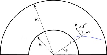
For a 2D circular arc geometry (figure 3), it is convenient to transform to polar coordinates
 $(r,\unicode[STIX]{x1D703})$
. Specializing to the zero level-set curve, we now define the DSD surface as
 $$\begin{eqnarray}\displaystyle \unicode[STIX]{x1D713}=\unicode[STIX]{x1D703}-\unicode[STIX]{x1D703}_{s}(r,t)=0. & & \displaystyle\end{eqnarray}$$
Subsequently, equation (2.2) becomes
 $$\begin{eqnarray}\displaystyle \unicode[STIX]{x1D703}_{s,t}=\frac{D_{n}}{r}(r^{2}\unicode[STIX]{x1D703}_{s,r}^{2}+1)^{1/2}. & & \displaystyle\end{eqnarray}$$
With the unit surface normal in polar coordinates given by
 $$\begin{eqnarray}\displaystyle \bar{\boldsymbol{n}}=\frac{(-r\unicode[STIX]{x1D703}_{s,r},1)}{(1+r^{2}\unicode[STIX]{x1D703}_{s,r}^{2})^{1/2}}, & & \displaystyle\end{eqnarray}$$
the curvature is
 $$\begin{eqnarray}\displaystyle \unicode[STIX]{x1D705}=\unicode[STIX]{x1D735}\boldsymbol{\cdot }\bar{\boldsymbol{n}}=-\frac{r}{(r^{2}\unicode[STIX]{x1D703}_{s,r}^{2}+1)^{3/2}}\left(\unicode[STIX]{x1D703}_{s,rr}+\unicode[STIX]{x1D703}_{s,r}\left(r\unicode[STIX]{x1D703}_{s,r}^{2}+\frac{2}{r}\right)\right). & & \displaystyle\end{eqnarray}$$
The 2D circular arc geometry and its polar coordinate representation. A schematic DSD surface is shown in blue.

2.1 Steady solutions for 2D circular arc geometries
We now assume the DSD surface in the 2D arc geometry propagates steadily with a constant angular phase velocity given by
 $\unicode[STIX]{x1D714}_{0}$
. In order to construct the steady solutions to the system (2.5)–(2.7), it is convenient to transform to a surface normal angle formulation, where
 $\unicode[STIX]{x1D719}=\unicode[STIX]{x1D719}(r)$
is the angle between the surface normal
 $\bar{\boldsymbol{n}}$
and
 $\bar{\unicode[STIX]{x1D73D}}$
as shown in figure 3. In the
 $\unicode[STIX]{x1D719}$
representation, the steady structure is determined by the solution of
 $$\begin{eqnarray}\displaystyle D_{n}=\unicode[STIX]{x1D714}_{0}r\cos \unicode[STIX]{x1D719},\quad \frac{\text{d}\unicode[STIX]{x1D719}}{\text{d}r}=\frac{\unicode[STIX]{x1D705}_{s}}{\cos \unicode[STIX]{x1D719}},\quad \frac{\text{d}\unicode[STIX]{x1D703}_{s}}{\text{d}r}=-\frac{\tan \unicode[STIX]{x1D719}}{r}, & & \displaystyle\end{eqnarray}$$
where
 $$\begin{eqnarray}\displaystyle \cos \unicode[STIX]{x1D719}=\bar{\boldsymbol{n}}\boldsymbol{\cdot }\bar{\unicode[STIX]{x1D73D}}=\frac{1}{(1+r^{2}\unicode[STIX]{x1D703}_{s,r}^{2})^{1/2}},\quad \sin \unicode[STIX]{x1D719}=\bar{\boldsymbol{n}}\boldsymbol{\cdot }\bar{\boldsymbol{r}}=-\frac{r\unicode[STIX]{x1D703}_{s,r}}{(1+r^{2}\unicode[STIX]{x1D703}_{s,r}^{2})^{1/2}}. & & \displaystyle\end{eqnarray}$$
The curvature component
 $\unicode[STIX]{x1D705}_{s}=\text{d}\unicode[STIX]{x1D719}/\text{d}\unicode[STIX]{x1D709}$
, where
 $\unicode[STIX]{x1D709}$
is a surface arc length coordinate, and is given by
 $$\begin{eqnarray}\displaystyle \unicode[STIX]{x1D705}_{s}=-\frac{(\unicode[STIX]{x1D703}_{s,r}+r\unicode[STIX]{x1D703}_{s,rr})}{(1+r^{2}\unicode[STIX]{x1D703}_{s,r}^{2})^{3/2}}. & & \displaystyle\end{eqnarray}$$
The total surface curvature is then
 $$\begin{eqnarray}\displaystyle \unicode[STIX]{x1D705}=\unicode[STIX]{x1D705}_{s}+\frac{\sin \unicode[STIX]{x1D719}}{r}, & & \displaystyle\end{eqnarray}$$
where, geometrically, the second term on the right corresponds to the rate of change of polar angle with arclength moving along the surface.
On the inner arc
 $r=R_{i}$
, we apply a fixed edge angle condition in all cases,
 $$\begin{eqnarray}\displaystyle \unicode[STIX]{x1D719}=\unicode[STIX]{x1D719}_{i}\quad \text{at }r=R_{i}, & & \displaystyle\end{eqnarray}$$
where
 $\unicode[STIX]{x1D719}$
is defined so that
 $\unicode[STIX]{x1D719}_{i}<0$
. We consider first the application of two boundary conditions on the outer arc,
 $r=R_{e}$
, one of which is designed for the DSD model to mimic a supersonic outflow condition on the outer arc. Specifically, an imposed fixed edge angle is represented by
 $$\begin{eqnarray}\displaystyle \unicode[STIX]{x1D719}=\unicode[STIX]{x1D719}_{e}\quad \text{at }r=R_{e}, & & \displaystyle\end{eqnarray}$$
where
 $\unicode[STIX]{x1D719}_{e}>0$
. Imposing zero curvature (as discussed in § 1) on the shape of the wave at the outer boundary gives
 $$\begin{eqnarray}\displaystyle \frac{\text{d}\unicode[STIX]{x1D719}}{\text{d}r}=-\frac{\tan \unicode[STIX]{x1D719}}{r}\quad \text{at }r=R_{e}. & & \displaystyle\end{eqnarray}$$
The steady solutions for a specific arc geometry where the radii of the inner and outer arc dimensions are specified are obtained as follows. Equations (2.8) are integrated between
 $r=R_{i}$
and
 $r=R_{e}$
and the steady structure and angular surface speed
 $\unicode[STIX]{x1D714}_{0}$
are calculated by a shooting method, imposing (2.12) on
 $r=R_{i}$
and either one of (2.13) or (2.14) on
 $r=R_{e}$
. Specifically, with the fixed angle condition (2.13) imposed on
 $r=R_{e}$
, an initial guess is made for
 $\unicode[STIX]{x1D714}_{0}$
, and (2.8) are integrated backwards towards
 $r=R_{i}$
, with the value of
 $\unicode[STIX]{x1D714}_{0}$
iterated on until the inner arc fixed angle condition (2.12) is met to some specified level of accuracy. The need to integrate from
 $r=R_{e}$
to
 $r=R_{i}$
, rather than the other way round, was motivated by the results of the asymptotic analysis discussed below. When the zero curvature condition (2.14) is imposed on
 $r=R_{e}$
, an initial guess is made for both
 $\unicode[STIX]{x1D714}_{0}$
and the edge angle
 $\unicode[STIX]{x1D719}$
at
 $r=R_{e}$
, and (2.8) are integrated towards
 $r=R_{i}$
, with the value of
 $\unicode[STIX]{x1D714}_{0}$
and
 $\unicode[STIX]{x1D719}$
at
 $r=R_{e}$
iterated on until the inner arc fixed angle condition (2.12) and zero curvature condition (2.14) are simultaneously satisfied. An alternative condition to the zero curvature assumption for the continuation solution is proposed below in § 3.1 based both on solutions of the steady-state model and on the results of an asymptotic analysis (presented in § 3.2).
3 Linear
 $D_{n}$
–
$\unicode[STIX]{x1D705}$
model


We start by examining the properties of arc geometry steady DSD surface propagation for the linear
 $D_{n}$
–
 $\unicode[STIX]{x1D705}$
relation,
 $$\begin{eqnarray}\displaystyle \frac{D_{n}}{D_{CJ}}=1-B\unicode[STIX]{x1D705}. & & \displaystyle\end{eqnarray}$$
This form allows for the development of an asymptotic solution (§ 3.2) that can be compared with the numerical solutions below. The values
 $D_{CJ}=0.78~\text{cm}~\unicode[STIX]{x03BC}\text{s}^{-1}$
and
 $B=0.1$
cm are taken. The parameter
 $D_{CJ}$
is equivalent to a Chapman–Jouguet (CJ) planar detonation velocity, while the parameter
 $B$
is broadly representative of a reaction zone thickness (in this case equal to 1 mm). These values have been used for verification studies of a recently developed body-fitted DSD implementation (Meyer et al.
Reference Meyer, Quirk, Short and Chiquete2016). We emphasize that it is not our intent in this section to replicate the behaviour of detonation propagation in any particular high explosive, but rather to provide insight on the striking properties of a simplified DSD model for describing detonation propagation in a circular arc geometry via both numerical and asymptotic analysis. That said, we show in § 4 that an appropriately calibrated linear
 $D_{n}$
–
 $\unicode[STIX]{x1D705}$
model does provide a surprisingly accurate representation of detonation propagation in a 2D circular arc validation experiment (Bdzil et al.
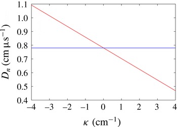
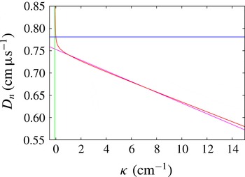
Reference Bdzil, Aslam, Henninger and Quirk2003) for PBX 9502. Figure 4 shows the
 $D_{n}$
variation with
 $\unicode[STIX]{x1D705}$
relative to the fixed
 $D_{CJ}$
value, extended into the negative curvature regime. We consider two generic choices for the edge angles that may be applied on either the inner or outer arc boundaries. For weak confinement, we choose a characteristic confinement (sonic) angle of 0.7 rad (characteristic of a high explosive confined by air or plastic), while for strong confinement we choose a confinement angle of 0.2 rad (characteristic of a high explosive confined by a metal, such as steel or copper).
The
 $D_{n}$
–
 $\unicode[STIX]{x1D705}$
linear relation (3.1) (red line). The CJ velocity
 $D_{CJ}=0.78~\text{cm}~\unicode[STIX]{x03BC}\text{s}^{-1}$
is shown by the blue line.

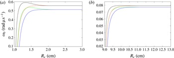
Surface angular speed variation as a function of outer radius
 $R_{e}$
for an inner radius (a)
 $R_{i}=1$
cm and (b)
 $R_{i}=9$
cm. Confinement angles are
 $\unicode[STIX]{x1D719}_{i}=-0.7$
on
 $r=R_{i}$
with
 $\unicode[STIX]{x1D719}_{e}=0.2$
(green line) and
 $\unicode[STIX]{x1D719}_{e}=0.7$
(blue line) on
 $r=R_{e}$
, and
 $\unicode[STIX]{x1D719}_{i}=-0.2$
on
 $r=R_{i}$
with
 $\unicode[STIX]{x1D719}_{e}=0.2$
(black line) and
 $\unicode[STIX]{x1D719}_{e}=0.7$
(orange line) on
 $r=R_{e}$
.

3.1 Arc results
Figure 5 shows the angular speed of steady surface wave propagation in an arc as a function of outer radius for two fixed inner radii,
 $R_{i}=1$
cm and
 $R_{i}=9$
cm, and the four different combinations of confinement angles. There are a number of properties to highlight. First we note that, as expected, the magnitude of
 $\unicode[STIX]{x1D714}_{0}$
is significantly smaller for the larger inner radius case
 $R_{i}=9$
cm. For sufficiently thin arcs, where
 $(R_{e}-R_{i})/R_{i}$
is small, the angular speed varies rapidly with small changes in
 $R_{e}$
. Moreover,
 $\unicode[STIX]{x1D714}_{0}$
depends on
 $R_{i}$
,
 $R_{e}$
,
 $\unicode[STIX]{x1D719}_{i}$
and
 $\unicode[STIX]{x1D719}_{e}$
. We also note that for thin arcs, when a confinement of
 $\unicode[STIX]{x1D719}_{i}=-0.2$
on the inner arc and
 $\unicode[STIX]{x1D719}_{e}=0.7$
on the outer arc is swapped with a confinement of
 $\unicode[STIX]{x1D719}_{i}=-0.7$
on the inner arc and
 $\unicode[STIX]{x1D719}_{e}=0.2$
on the outer arc with
 $R_{i}$
and
 $R_{e}$
fixed,
 $\unicode[STIX]{x1D714}_{0}$
is approximately the same. This points to a symmetry in the surface wave structure under the transformation
 $\unicode[STIX]{x1D719}_{i}\rightarrow -\unicode[STIX]{x1D719}_{e}$
,
 $\unicode[STIX]{x1D719}_{e}\rightarrow -\unicode[STIX]{x1D719}_{i}$
. Of particular interest, we observe in all cases that, as the arc becomes sufficiently thick, the angular speed becomes independent of the size of the outer arc
 $R_{e}$
. In addition, it also becomes independent of the outer arc confinement angle, as demonstrated by the merging of the two solutions for
 $\unicode[STIX]{x1D719}_{i}=-0.2$
and
 $\unicode[STIX]{x1D719}_{e}=0.2$
and
 $\unicode[STIX]{x1D719}_{e}=0.7$
and for the two solutions for
 $\unicode[STIX]{x1D719}_{i}=-0.7$
and
 $\unicode[STIX]{x1D719}_{e}=0.2$
and
 $\unicode[STIX]{x1D719}_{e}=0.7$
(for each
 $R_{i}$
). Thus, for sufficiently thick arcs,
 $\unicode[STIX]{x1D714}_{0}$
appears to depend only on
 $R_{i}$
and
 $\unicode[STIX]{x1D719}_{i}$
, even though we are enforcing a specific confinement angle on the outer arc. We also note that the difference in magnitude in
 $\unicode[STIX]{x1D714}_{0}$
between strong inner confinement and weak inner confinement when
 $\unicode[STIX]{x1D714}_{0}$
becomes independent of
 $R_{e}$
and
 $\unicode[STIX]{x1D719}_{e}$
is comparatively small, possibly indicating only a weak dependence of
 $\unicode[STIX]{x1D714}_{0}$
on
 $\unicode[STIX]{x1D719}_{i}$
. Finally, it is also interesting to note that
 $\unicode[STIX]{x1D714}_{0}$
increases monotonically with
 $R_{e}$
limiting to a constant for weak outer arc confinement,
 $\unicode[STIX]{x1D719}_{e}=0.7$
, but develops a maximum for some intermediate value of
 $R_{e}$
for strong outer arc confinement,
 $\unicode[STIX]{x1D719}_{e}=0.2$
.
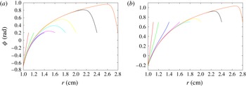
Surface normal angle variation as a function of
 $r$
for
 $R_{i}=1$
cm. Confinement angles are (a)
 $\unicode[STIX]{x1D719}_{i}=-0.7$
,
 $\unicode[STIX]{x1D719}_{e}=0.2$
, and (b)
 $\unicode[STIX]{x1D719}_{i}=-0.2$
,
 $\unicode[STIX]{x1D719}_{e}=0.7$
.

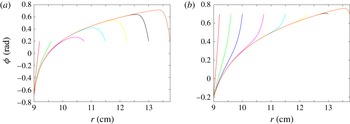
Surface normal angle variation as a function of
 $r$
for
 $R_{i}=9$
cm. Confinement angles are (a)
 $\unicode[STIX]{x1D719}_{i}=-0.7$
,
 $\unicode[STIX]{x1D719}_{e}=0.2$
, and (b)
 $\unicode[STIX]{x1D719}_{i}=-0.2$
,
 $\unicode[STIX]{x1D719}_{e}=0.7$
.

Figures 6 and 7 show the surface normal angle
 $(\unicode[STIX]{x1D719})$
variation with
 $r$
for various arc outer radii (
 $R_{e}$
) for
 $R_{i}=1$
cm and
 $R_{i}=9$
cm for two confinement angle cases (
 $\unicode[STIX]{x1D719}_{i}=-0.7$
,
 $\unicode[STIX]{x1D719}_{e}=0.2$
and
 $\unicode[STIX]{x1D719}_{i}=-0.2$
,
 $\unicode[STIX]{x1D719}_{e}=0.7$
). In each case, for sufficiently small
 $R_{e}$
,
 $\unicode[STIX]{x1D719}$
increases monotonically across the arc with no overlap in the solution profiles for increasing
 $R_{e}$
. As
 $R_{e}$
increases, we observe that the solution profiles start to overlap in the inner and central parts of the arc, only diverging in the region near
 $r=R_{e}$
to meet the enforced confinement angle condition on
 $r=R_{e}$
. For sufficiently large
 $R_{e}$
, there is also a region interior to the arc where
 $\unicode[STIX]{x1D719}$
exceeds the value of
 $\unicode[STIX]{x1D719}_{e}$
before relaxing to
 $\unicode[STIX]{x1D719}_{e}$
at
 $r=R_{e}$
. Moreover, as
 $R_{e}$
increases, the variation in
 $\unicode[STIX]{x1D719}$
with
 $r$
near
 $r=R_{e}$
takes on the form of a boundary layer. Significantly, the values of
 $R_{e}$
for which the
 $\unicode[STIX]{x1D719}$
variation with
 $r$
begin to overlap approximately coincide with the values of
 $R_{e}$
where
 $\unicode[STIX]{x1D714}_{0}$
becomes independent of
 $R_{e}$
and
 $\unicode[STIX]{x1D719}_{e}$
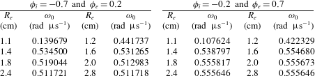
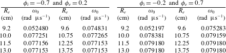
. Tables 1 and 2 show the variation in
 $\unicode[STIX]{x1D714}_{0}$
for each of the profiles shown in figures 6 and 7. For
 $R_{i}=1$
cm,
 $\unicode[STIX]{x1D714}_{0}$
approaches a constant for
 $R_{e}\geqslant 1.8$
cm, while for
 $R_{i}=9$
cm,
 $\unicode[STIX]{x1D714}_{0}$
approaches a constant for
 $R_{e}\geqslant 10$
cm. Thus the boundary layers near
 $r=R_{e}$
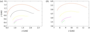
appear to have minimal effect on the angular speed, a property explained through the asymptotic analysis presented in § 3.2. Figure 8 shows some of the surface wave shapes corresponding to solutions presented in figures 6(a) and 7(a) in planar coordinates. Below, we further explore the relationship between the structure and speed of the surface solutions for various arc size and confinement conditions.
Surface wave shape in planar coordinates
 $(x,y)$
corresponding to some of the solutions shown in figures 6(a) and 7(a). The surfaces are oriented such that the points
 $r=R_{e}$
lie along
 $\unicode[STIX]{x1D703}=\unicode[STIX]{x03C0}/8$
. Shown in (a) are surfaces for
 $R_{i}=1$
cm and
 $R_{e}=1.2$
,
 $1.6$
,
 $2.0$
,
 $2.4$
and
 $2.8$
cm, while those in (b) are for
 $R_{i}=9$
cm and
 $R_{e}=9.6$
,
 $10.75$
,
 $12.25$
and
 $13.75$
cm.

Surface angular speed variation with
 $R_{e}$
for
 $R_{i}=1$
cm.

Surface angular speed variation with
 $R_{e}$
for
 $R_{i}=9$
cm.

Steady DSD solutions for the linear
 $D_{n}$
–
 $\unicode[STIX]{x1D705}$
relation (3.1) with
 $R_{i}=1$
cm and
 $R_{e}=1.2$
cm. Confinement angles are
 $\unicode[STIX]{x1D719}_{i}=-0.7$
on
 $r=R_{i}$
with
 $\unicode[STIX]{x1D719}_{e}=0.7$
(blue line,
 $\unicode[STIX]{x1D714}_{0}=0.271306$
) and
 $\unicode[STIX]{x1D719}_{e}=0.2$
(green line,
 $\unicode[STIX]{x1D714}_{0}=0.441737$
) on
 $r=R_{e}$
, and
 $\unicode[STIX]{x1D719}_{i}=-0.2$
on
 $r=R_{i}$
with
 $\unicode[STIX]{x1D719}_{e}=0.7$
(orange line,
 $\unicode[STIX]{x1D714}_{0}=0.422329$
) and
 $\unicode[STIX]{x1D719}_{e}=0.2$
(black line,
 $\unicode[STIX]{x1D714}_{0}=0.570747$
) on
 $r=R_{e}$
.

Steady DSD solutions for the linear
 $D_{n}$
–
 $\unicode[STIX]{x1D705}$
relation (3.1) with
 $R_{i}=9$
cm and
 $R_{e}=9.2$
cm. Confinement angles are
 $\unicode[STIX]{x1D719}_{i}=-0.7$
on
 $r=R_{i}$
with
 $\unicode[STIX]{x1D719}_{e}=0.7$
(blue line,
 $\unicode[STIX]{x1D714}_{0}=0.032845$
) and
 $\unicode[STIX]{x1D719}_{e}=0.2$
(green line,
 $\unicode[STIX]{x1D714}_{0}=0.052480$
) on
 $r=R_{e}$
, and
 $\unicode[STIX]{x1D719}_{i}=-0.2$
on
 $r=R_{i}$
with
 $\unicode[STIX]{x1D719}_{e}=0.7$
(orange line,
 $\unicode[STIX]{x1D714}_{0}=0.052197$
) and
 $\unicode[STIX]{x1D719}_{e}=0.2$
(black line,
 $\unicode[STIX]{x1D714}_{0}=0.069131$
) on
 $r=R_{e}$
.

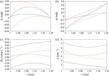
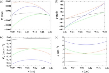
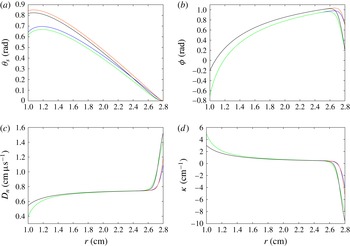
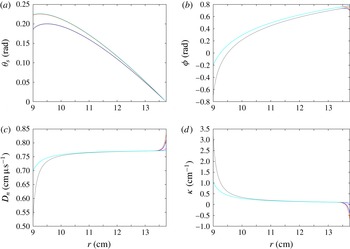
Figures 9 and 10 show the variation in polar angle surface shape (
 $\unicode[STIX]{x1D703}_{s}$
), the surface normal angle
 $(\unicode[STIX]{x1D719})$
, the normal surface velocity (
 $D_{n}$
) and surface curvature (
 $\unicode[STIX]{x1D705}$
) as a function of
 $r$
for thin arc cases
 $R_{i}=1$
cm with
 $R_{e}=1.2$
cm and
 $R_{i}=9$
cm with
 $R_{e}=9.2$
cm for the four different inner and outer arc confinement angle arrangements. For these thin arc cases, the variations in amplitude of
 $D_{n}$
and
 $\unicode[STIX]{x1D705}$
across the arc are only moderate. However, the magnitudes of
 $D_{n}$
and
 $\unicode[STIX]{x1D705}$
vary significantly with confinement, with the strong confinement case
 $\unicode[STIX]{x1D719}_{i}=-0.2$
and
 $\unicode[STIX]{x1D719}_{e}=0.2$
having the smallest curvature and largest normal surface velocity. We note an approximate symmetry in the
 $D_{n}$
and
 $\unicode[STIX]{x1D705}$
fields about the radial midpoint for the confinement cases
 $\unicode[STIX]{x1D719}_{i}=-0.2$
,
 $\unicode[STIX]{x1D719}_{e}=0.7$
and
 $\unicode[STIX]{x1D719}_{i}=-0.7$
,
 $\unicode[STIX]{x1D719}_{e}=0.2$
. The curvature is positive in all cases, and thus
 $D_{n}<D_{CJ}$
across the arc. The surface normal angle increases monotonically from the inner arc radius to the outer arc radius. The surface shapes have been centred so that
 $\unicode[STIX]{x1D703}_{s}=0$
at
 $r=R_{e}$
. For the same confinement on the inner and outer arcs, the surface shapes are approximately symmetric about the arc midpoint, but for
 $\unicode[STIX]{x1D719}_{i}=-0.2$
and
 $\unicode[STIX]{x1D719}_{e}=0.7$
the surface on the inner arc leads that on the outer arc. For
 $\unicode[STIX]{x1D719}_{i}=-0.7$
and
 $\unicode[STIX]{x1D719}_{e}=0.2$
, however, the situation is reversed.
Steady DSD solutions for the linear
 $D_{n}$
–
 $\unicode[STIX]{x1D705}$
relation (3.1) with
 $R_{i}=1$
cm and
 $R_{e}=2.8$
cm. Confinement angles are
 $\unicode[STIX]{x1D719}_{i}=-0.7$
on
 $r=R_{i}$
with
 $\unicode[STIX]{x1D719}_{e}=0.7$
(blue line,
 $\unicode[STIX]{x1D714}_{0}=0.511718$
) and
 $\unicode[STIX]{x1D719}_{e}=0.2$
(green line,
 $\unicode[STIX]{x1D714}_{0}=0.511718$
) on
 $r=R_{e}$
, and
 $\unicode[STIX]{x1D719}_{i}=-0.2$
on
 $r=R_{i}$
with
 $\unicode[STIX]{x1D719}_{e}=0.7$
(orange line,
 $\unicode[STIX]{x1D714}_{0}=0.555646$
) and
 $\unicode[STIX]{x1D719}_{e}=0.2$
(black line,
 $\unicode[STIX]{x1D714}_{0}=0.555646$
) on
 $r=R_{e}$
.

Steady DSD solutions for the linear
 $D_{n}$
–
 $\unicode[STIX]{x1D705}$
relation (3.1) with
 $R_{i}=9$
cm and
 $R_{e}=13.75$
cm. Confinement angles are
 $\unicode[STIX]{x1D719}_{i}=-0.7$
on
 $r=R_{i}$
with
 $\unicode[STIX]{x1D719}_{e}=0.7$
(blue line,
 $\unicode[STIX]{x1D714}_{0}=0.077153$
) and
 $\unicode[STIX]{x1D719}_{e}=0.2$
(green line,
 $\unicode[STIX]{x1D714}_{0}=0.077153$
) and
 $\unicode[STIX]{x1D719}_{i}=-0.2$
on
 $r=R_{i}$
with
 $\unicode[STIX]{x1D719}_{e}=0.7$
(orange line,
 $\unicode[STIX]{x1D714}_{0}=0.079180$
) and
 $\unicode[STIX]{x1D719}_{e}=0.2$
(black line,
 $\unicode[STIX]{x1D714}_{0}=0.079180$
) on
 $r=R_{e}$
.

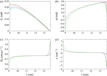
Figures 11 and 12 show the variation in the polar angle surface shape (
 $\unicode[STIX]{x1D703}_{s}$
), the surface normal angle
 $(\unicode[STIX]{x1D719})$
, the normal surface velocity
 $D_{n}$
and surface curvature (
 $\unicode[STIX]{x1D705}$
) as a function of
 $r$
for the thick arc cases
 $R_{i}=1$
cm with
 $R_{e}=2.8$
cm and
 $R_{i}=9$
cm with
 $R_{e}=13.75$
cm for the four different inner and outer arc confinement angle arrangements. The solutions for
 $\unicode[STIX]{x1D719}_{i}=-0.2$
with
 $\unicode[STIX]{x1D719}_{e}=0.2$
or
 $\unicode[STIX]{x1D719}_{e}=0.7$
have the same angular speed, as do the two solutions with
 $\unicode[STIX]{x1D719}_{i}=-0.7$
with
 $\unicode[STIX]{x1D719}_{e}=0.2$
or
 $\unicode[STIX]{x1D719}_{e}=0.7$
. Both the
 $D_{n}$
and
 $\unicode[STIX]{x1D705}$
solutions show a moderately strong variation with
 $r$
near the inner arc, a weaker variation in the central part of the arc, and then a strong variation near the outer arc. This behaviour is again explained through the asymptotic analysis presented in § 3.2. Near the inner arc, the
 $D_{n}$
and
 $\unicode[STIX]{x1D705}$
variations with
 $r$
for the two profiles for
 $\unicode[STIX]{x1D719}_{i}=-0.2$
with
 $\unicode[STIX]{x1D719}_{e}=0.2$
and
 $\unicode[STIX]{x1D719}_{e}=0.7$
overlap, as do the variations for the two profiles for
 $\unicode[STIX]{x1D719}_{i}=-0.7$
with
 $\unicode[STIX]{x1D719}_{e}=0.2$
and
 $\unicode[STIX]{x1D719}_{e}=0.7$
. In the central part of the arc, all four solutions merge. In this central region, the curvature is moderately small, and the normal surface velocity is approximately
 $D_{CJ}$
. Near
 $r=R_{e}$
, we again see rapid variations in
 $D_{n}$
and
 $\unicode[STIX]{x1D705}$
. The two solutions for
 $\unicode[STIX]{x1D719}_{e}=0.7$
and
 $\unicode[STIX]{x1D719}_{i}=-0.2$
and
 $\unicode[STIX]{x1D719}_{i}=-0.7$
are moderately close in the rapid variation region near
 $r=R_{e}$
, as are the two solutions for
 $\unicode[STIX]{x1D719}_{e}=0.2$
and
 $\unicode[STIX]{x1D719}_{i}=-0.2$
and
 $\unicode[STIX]{x1D719}_{i}=-0.7$
. In addition, in order to meet the imposed angle on the outer arc, the surface shape has to acquire significant negative curvature in the layer near
 $r=R_{e}$
. This corresponds to a section of the surface wave that is divergent, where
 $D_{n}>D_{CJ}$
. In the follow-up paper detailing reactive burn modelling of detonation propagation in the arc geometry, we will show that negatively curved sections of the lead detonation shock in an arc geometry can arise as a result of shock reflection near a high-impedance confiner, either through a smoothly varying von Neumann reflection or as a classical Mach reflection of the incident detonation shock. The surface normal angle variation for the two solutions for
 $\unicode[STIX]{x1D719}_{i}=-0.2$
with
 $\unicode[STIX]{x1D719}_{e}=0.2$
and
 $\unicode[STIX]{x1D719}_{e}=0.7$
overlap for most of the arc thickness, except near
 $r=R_{e}$
, as do the two solutions for
 $\unicode[STIX]{x1D719}_{i}=-0.7$
with
 $\unicode[STIX]{x1D719}_{e}=0.2$
and
 $\unicode[STIX]{x1D719}_{e}=0.7$
. The surface shapes have again been centred so that
 $\unicode[STIX]{x1D703}_{s}=0$
at
 $r=R_{e}$
. For the thicker arcs, the surface at the inner arc leads that on the outer arc in all cases. As noted above, an interesting feature of the angular speed variation as a function of outer radius
 $R_{e}$
for strong confinement on the outer boundary
 $(\unicode[STIX]{x1D719}_{e}=0.2)$
(see figure 5) is that the steady-state speed has a maximum for some intermediate value of
 $R_{e}$
. In a simpler 2D slab or axisymmetric rate-stick geometry, the axial phase speed increases with increases in the charge size and increases in the degree of confinement (Jackson & Short Reference Jackson and Short2015). For the arc geometry, it is apparent that the angular speed is not influenced by either
 $\unicode[STIX]{x1D719}_{e}$
or
 $R_{e}$
for sufficiently large arc thicknesses. The observed variation in
 $\unicode[STIX]{x1D714}_{0}$
indicates that, for strong outer arc confinement, a balance is achieved between arc thickness and the influence of the outer confinement on speed that leads to a maximum at an intermediate value of
 $R_{e}$
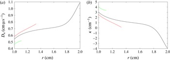
. Figure 13 shows a comparison of the
 $D_{n}$
and
 $\unicode[STIX]{x1D705}$
variation with strong confinement on the inner and outer boundaries (
 $\unicode[STIX]{x1D719}_{i}=-0.2$
,
 $\unicode[STIX]{x1D719}_{e}=0.2$
) with
 $R_{i}=1$
cm and three values of
 $R_{e}$
, one corresponding to a case of attaining a limiting value of
 $\unicode[STIX]{x1D714}_{0}$
at large charge size (
 $R_{e}=2$
cm), one corresponding to an
 $R_{e}$
close to the observed maximum in
 $\unicode[STIX]{x1D714}_{0}$
(
 $R_{e}=1.33$
cm) and the other corresponding to a small charge size with
 $\unicode[STIX]{x1D714}_{0}$
lower than the large charge size limit (
 $R_{e}=1.11$
cm). In the asymptotic analysis presented below, we show that, for large charge sizes, the deviations of the angular speed from a Huygens limit is determined by the behaviour in a narrow boundary layer near
 $r=R_{i}$
. Comparing the
 $D_{n}$
and
 $\unicode[STIX]{x1D705}$
behaviour for the three charge sizes, we note that for
 $R_{e}=1.33$
cm,
 $D_{n}$
is uniformly larger, while
 $\unicode[STIX]{x1D705}$
is uniformly smaller, than the values for
 $R_{e}=2$
near
 $r=R_{i}$
. On the other hand, for
 $R_{e}=1.11$
cm,
 $D_{n}$
is uniformly smaller, while
 $\unicode[STIX]{x1D705}$
is uniformly larger, than the values for
 $R_{e}=2$
near
 $r=R_{i}$
. This indicates why
 $\unicode[STIX]{x1D714}_{0}$
is larger at the intermediate value of
 $R_{e}$
.
Comparison of (a)
 $D_{n}$
and (b)
 $\unicode[STIX]{x1D705}$
variation with strong confinement on the inner and outer boundaries (
 $\unicode[STIX]{x1D719}_{i}=-0.2$
,
 $\unicode[STIX]{x1D719}_{e}=0.2$
) with
 $R_{i}=1$
cm and
 $R_{e}=1.11$
cm (green line),
 $R_{e}=1.33$
cm (red line) and
 $R_{e}=2$
cm (black line). For
 $R_{e}=1.11$
cm,
 $\unicode[STIX]{x1D714}_{0}=0.475003$
, for
 $R_{e}=1.33$
cm,
 $\unicode[STIX]{x1D714}_{0}=0.591080$
, and for
 $R_{e}=2$
cm,
 $\unicode[STIX]{x1D714}_{0}=0.555932$
.

We return now to the discussion in § 1, where we noted that the parabolic DSD model has no notion of sound speed, and therefore supersonic or subsonic flow at the HE/confiner interface. The calculations above show that, for sufficiently thick arcs, the angular speed of the wave becomes independent of both
 $R_{e}$
and
 $\unicode[STIX]{x1D719}_{e}$
. Owing to the lack of influence of
 $R_{e}$
and
 $\unicode[STIX]{x1D719}_{e}$
on
 $\unicode[STIX]{x1D714}_{0}$
, the DSD model can be thought of as having a property in an arc geometry that mimics the effect of a supersonic outflow condition at the outer arc boundary. As noted in § 1, in the DSD model described by Bdzil et al. (Reference Bdzil, Henninger and Walter2006, Reference Bdzil, Aida, Henninger and Walter2007) and Hernández et al. (Reference Hernández, Bdzil and Stewart2013), a supersonic outflow-style condition is modelled by employing a zero curvature condition on the wave shape at the outer arc. However, the overlap of the solutions in the interior of the arc as
 $R_{e}$
increases, as seen in figures 6 and 7, provides motivation for the use of an alternative continuation boundary condition on the outer arc to mimic a supersonic-like outflow condition. Owing to the observed overlapping behaviour, the proposed continuation condition amounts to conducting a DSD calculation with the same outer arc confinement but now for an outer arc radius
 $R_{e}+\unicode[STIX]{x0394}R_{e}$
, where the buffer layer
 $\unicode[STIX]{x0394}R_{e}>0$
is chosen such that the solution in the region
 $0\leqslant r\leqslant R_{e}$
is unaffected by further increases in
 $\unicode[STIX]{x0394}R_{e}$
(see figures 6 and 7). The solution for
 $0\leqslant r\leqslant R_{e}$
is then extracted from the larger domain. In summary, we apply the fixed angle condition (2.13) at a distance
 $r=R_{e}+\unicode[STIX]{x0394}R_{e}>R_{e}$
such that further increases in the magnitude of
 $\unicode[STIX]{x0394}R_{e}$
do not change the surface shape in the arc region
 $R_{i}\leqslant r\leqslant R_{e}$
, i.e.
 $$\begin{eqnarray}\displaystyle \unicode[STIX]{x1D719}=\unicode[STIX]{x1D719}_{e}\quad \text{at }r=R_{e}+\unicode[STIX]{x0394}R_{e}. & & \displaystyle\end{eqnarray}$$
For the continuation condition (3.2), a similar procedure for numerical integration of the steady equations (2.8) to that described in § 2.1 is adopted, except that the integration now starts from
 $r=R_{e}+\unicode[STIX]{x0394}R_{e}$
. Further support for the use of this style of continuation condition is provided in the asymptotic analysis presented below.
Steady DSD solutions for the linear
 $D_{n}$
–
 $\unicode[STIX]{x1D705}$
relation (3.1) with
 $R_{i}=1$
cm and
 $R_{e}=2.8$
cm. Confinement conditions are
 $\unicode[STIX]{x1D719}_{i}=-0.7$
on
 $r=R_{i}$
with
 $\unicode[STIX]{x1D719}_{e}=0.7$
(dark blue line), the zero curvature assumption (yellow line) and the continuation solution (grey line) on
 $r=R_{e}$
. In all cases
 $\unicode[STIX]{x1D714}_{0}=0.511718$
. Also shown are confinement conditions
 $\unicode[STIX]{x1D719}_{i}=-0.2$
on
 $r=R_{i}$
with
 $\unicode[STIX]{x1D719}_{e}=0.7$
(orange line), the zero curvature assumption (magenta line) and the continuation solution (light blue line) on
 $r=R_{e}$
. In all cases
 $\unicode[STIX]{x1D714}_{0}=0.555646$
.

Steady DSD solutions for the linear
 $D_{n}$
–
 $\unicode[STIX]{x1D705}$
relation (3.1) with
 $R_{i}=9$
cm and
 $R_{e}=13.75$
cm. Confinement conditions are
 $\unicode[STIX]{x1D719}_{i}=-0.7$
on
 $r=R_{i}$
with
 $\unicode[STIX]{x1D719}_{e}=0.7$
(dark blue line), the zero curvature assumption (yellow line) and the continuation solution (grey line) on
 $r=R_{e}$
. In all cases
 $\unicode[STIX]{x1D714}_{0}=0.077153$
. Also shown are confinement conditions
 $\unicode[STIX]{x1D719}_{i}=-0.2$
on
 $r=R_{i}$
with
 $\unicode[STIX]{x1D719}_{e}=0.7$
(orange line), the zero curvature condition (magenta line) and the continuation solution (light blue line) on
 $r=R_{e}$
. In all cases
 $\unicode[STIX]{x1D714}_{0}=0.079180$
.

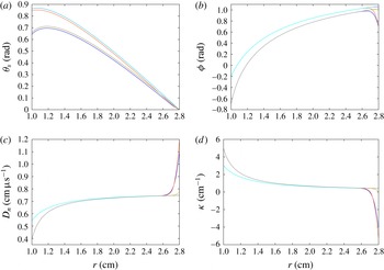
Figures 14 (
 $R_{i}=1$
cm and
 $R_{e}=2.8$
cm) and 15 (
 $R_{i}=9$
cm and
 $R_{e}=13.75$
cm) show comparisons between steady solutions for
 $\unicode[STIX]{x1D719}_{i}=-0.7$
and
 $\unicode[STIX]{x1D719}_{i}=-0.2$
for each of the three different conditions on
 $r=R_{e}$
, namely imposed angle
 $(\unicode[STIX]{x1D719}_{e}=0.7)$
, zero curvature and continuation. For these arc thicknesses, we again find that the specific type of boundary condition on the outer arc does not influence
 $\unicode[STIX]{x1D714}_{0}$
to the significant figures shown. For the imposed angle condition on
 $r=R_{e}$
, we observe in each case, as before, a boundary layer in which both
 $D_{n}$
and
 $\unicode[STIX]{x1D705}$
vary rapidly. The curvature is negative in this region, and consequently
 $D_{n}>D_{CJ}$
. For the zero curvature boundary condition, we still observe a boundary layer near
 $r=R_{e}$
in each case, but the
 $D_{n}$
and
 $\unicode[STIX]{x1D705}$
variations are significantly reduced in magnitude relative to the imposed angle condition. Also, for the zero curvature condition on
 $r=R_{e}$
, the surface curvatures are positive for
 $R_{i}\leqslant r<R_{e}$
, and thus
 $D_{n}$
remains below
 $D_{CJ}$
for
 $R_{i}\leqslant r<R_{e}$
, while
 $D_{n}=D_{CJ}$
on
 $r=R_{e}$
. For the continuation condition, there is no boundary layer near
 $r=R_{e}$
in any case. The curvature is positive at
 $r=R_{e}$
, and thus the curvature is positive across the arc (
 $R_{i}\leqslant r\leqslant R_{e}$
). In terms of application to the DSD model, all three conditions can be reasonably argued to be suitable for a DSD model, although the zero curvature condition is a compromise to imposing a true continuation condition on the fixed domain (
 $R_{i}\leqslant r<R_{e}$
). Importantly, all three types of boundary conditions on the outer arc generate steady solutions, and deciding which one should be applied to the outer arc surface for a given geometry and confinement cannot be properly addressed within the context of the DSD model alone. This will require comparisons of a DSD model with a simulation of a reactive flow model, the subject of a future article, and will establish the most appropriate boundary conditions for the parabolic DSD model to mimic the properties of the hyperbolic reactive Euler model for a variety of confinement situations.
3.2 Asymptotic analysis
For the linear
 $D_{n}$
–
 $\unicode[STIX]{x1D705}$
relation (3.1), asymptotic expressions for the steady angular speed
 $\unicode[STIX]{x1D714}_{0}$
in an arc geometry are possible that also relate the radial variation of the surface shape to the surface normal angle. From (2.8), (2.11) and (3.1) we have that
 $$\begin{eqnarray}\displaystyle \unicode[STIX]{x1D705}=\frac{1}{B}\left(1-\frac{\unicode[STIX]{x1D714}_{0}r\cos \unicode[STIX]{x1D719}}{D_{CJ}}\right),\quad \unicode[STIX]{x1D705}_{s}=\frac{1}{B}\left(1-\frac{\unicode[STIX]{x1D714}_{0}r\cos \unicode[STIX]{x1D719}}{D_{CJ}}\right)-\frac{\sin \unicode[STIX]{x1D719}}{r}, & & \displaystyle\end{eqnarray}$$
while
 $r(\unicode[STIX]{x1D719})$
is determined from
 $$\begin{eqnarray}\displaystyle \left(1-\frac{\unicode[STIX]{x1D714}_{0}r\cos \unicode[STIX]{x1D719}}{D_{CJ}}-\frac{B\sin \unicode[STIX]{x1D719}}{r}\right)\frac{\text{d}r}{\text{d}\unicode[STIX]{x1D719}}=B\cos \unicode[STIX]{x1D719}. & & \displaystyle\end{eqnarray}$$
For the asymptotic analysis, we introduce the scaled quantities
 $$\begin{eqnarray}\displaystyle \hat{B}=\frac{B}{B_{ref}},\quad \hat{r}=\frac{r}{r_{ref}},\quad \hat{D}_{CJ}=\frac{D_{CJ}}{D_{ref}},\quad \hat{\unicode[STIX]{x1D705}}=\unicode[STIX]{x1D705}B_{ref}, & & \displaystyle\end{eqnarray}$$
where
 $B_{ref}$
and
 $r_{ref}$
are suitably defined reference lengths and
 $D_{ref}$
is a suitably defined reference velocity such that
 $\hat{B}$
,
 $\hat{r}$
and
 $\hat{D}_{CJ}$
are
 $O(1)$
. With these scalings, equation (3.4) becomes
 $$\begin{eqnarray}\displaystyle \left(1-\left(\frac{\unicode[STIX]{x1D714}_{0}r_{ref}}{D_{ref}}\right)\frac{\hat{r}\cos \unicode[STIX]{x1D719}}{\hat{D}_{CJ}}-\left(\frac{B_{ref}}{r_{ref}}\right)\frac{\hat{B}\sin \unicode[STIX]{x1D719}}{\hat{r}}\right)\frac{\text{d}\hat{r}}{\text{d}\unicode[STIX]{x1D719}}=\left(\frac{B_{ref}}{r_{ref}}\right)\hat{B}\cos \unicode[STIX]{x1D719}. & & \displaystyle\end{eqnarray}$$
Consequently, a non-dimensional angular velocity is introduced, where
 $$\begin{eqnarray}\displaystyle \hat{\unicode[STIX]{x1D714}}_{0}=\frac{\unicode[STIX]{x1D714}_{0}r_{ref}}{D_{ref}}, & & \displaystyle\end{eqnarray}$$
whereupon (3.6) becomes
 $$\begin{eqnarray}\displaystyle \left(1-\frac{\hat{\unicode[STIX]{x1D714}}_{0}\hat{r}\cos \unicode[STIX]{x1D719}}{\hat{D}_{CJ}}-\unicode[STIX]{x1D716}\frac{\hat{B}\sin \unicode[STIX]{x1D719}}{\hat{r}}\right)\frac{\text{d}\hat{r}}{\text{d}\unicode[STIX]{x1D719}}=\unicode[STIX]{x1D716}\hat{B}\cos \unicode[STIX]{x1D719}, & & \displaystyle\end{eqnarray}$$
with
 $$\begin{eqnarray}\displaystyle \unicode[STIX]{x1D716}=\frac{B_{ref}}{r_{ref}}. & & \displaystyle\end{eqnarray}$$
All we require for the asymptotic analysis is that
 $\unicode[STIX]{x1D716}\ll 1$
, i.e. that the ratio of the length scales
 $B_{ref}$
to
 $r_{ref}$
is small. Sensible choices for
 $B_{ref}$
and
 $r_{ref}$
would be
 $B_{ref}=B$
and
 $r_{ref}=R_{i}$
, in which case the scaling
 $\unicode[STIX]{x1D716}\ll 1$
would require that the reaction zone length scale
 $B$
be significantly smaller than the inner arc radius. In particular, this does not establish any requirements on the individual magnitudes of
 $B$
and
 $R_{i}$
, just that their ratio be small. Similarly, a sensible choice for
 $D_{ref}$
would be
 $D_{CJ}$
. However, there is no specific requirement for these choices of reference lengths and velocities, and thus in the following the specification is left as arbitrary, provided only that
 $\hat{B}$
,
 $\hat{r}$
and
 $\hat{D}_{CJ}$
are
 $O(1)$
. Returning to the surface curvature expression (2.11), in scaled form this becomes
 $$\begin{eqnarray}\displaystyle \hat{\unicode[STIX]{x1D705}}=\hat{\unicode[STIX]{x1D705}}_{s}+\unicode[STIX]{x1D716}\frac{\sin \unicode[STIX]{x1D719}}{\hat{r}}, & & \displaystyle\end{eqnarray}$$
where, as before, the first term on the right corresponds to the rate of change of
 $\unicode[STIX]{x1D719}$
with arclength, and the second the rate of change of polar angle with arclength along the surface. We show below that, in certain regimes of the arc, the total surface curvature
 $\hat{\unicode[STIX]{x1D705}}$
can vary by up to
 $O(1)$
amounts and thus, for
 $\unicode[STIX]{x1D716}\ll 1$
, in these situations, the dominant curvature contribution will arise from the rate of change of
 $\unicode[STIX]{x1D719}$
with arclength. In general,
 $$\begin{eqnarray}\displaystyle \hat{\unicode[STIX]{x1D705}}=\frac{1}{\hat{B}}\left(1-\frac{\hat{\unicode[STIX]{x1D714}}_{0}\hat{r}}{\hat{D}_{CJ}}\cos \unicode[STIX]{x1D719}\right),\quad \hat{D}_{n}=\hat{\unicode[STIX]{x1D714}}_{0}\hat{r}\cos \unicode[STIX]{x1D719}. & & \displaystyle\end{eqnarray}$$
3.2.1 Thin arc case
The first case we examine is a thin arc of explosive of thickness
 $O(\unicode[STIX]{x1D716})$
, i.e. where
 $\hat{R}_{e}-\hat{R}_{i}=O(\unicode[STIX]{x1D716})$
. We expand
 $\hat{r}$
and
 $\hat{\unicode[STIX]{x1D714}}_{0}$
as
 $$\begin{eqnarray}\displaystyle \hat{r}\sim \hat{R}_{i}+\unicode[STIX]{x1D716}\hat{r}_{1}+\unicode[STIX]{x1D716}^{2}\hat{r}_{2},\quad \hat{\unicode[STIX]{x1D714}}_{0}\sim \hat{\unicode[STIX]{x1D714}}_{00}+\unicode[STIX]{x1D716}\hat{\unicode[STIX]{x1D714}}_{01}. & & \displaystyle\end{eqnarray}$$
Substituting (3.12) into (3.8), we find at
 $O(\unicode[STIX]{x1D716})$
that
 $$\begin{eqnarray}\displaystyle \left(1-\frac{\hat{\unicode[STIX]{x1D714}}_{00}\hat{R}_{i}\cos \unicode[STIX]{x1D719}}{\hat{D}_{CJ}}\right)\frac{\text{d}\hat{r}_{1}}{\text{d}\unicode[STIX]{x1D719}}=\hat{B}\cos \unicode[STIX]{x1D719}, & & \displaystyle\end{eqnarray}$$
and at
 $O(\unicode[STIX]{x1D716}^{2})$
that
 $$\begin{eqnarray}\displaystyle \left(1-\frac{\hat{\unicode[STIX]{x1D714}}_{00}\hat{R}_{i}\cos \unicode[STIX]{x1D719}}{\hat{D}_{CJ}}\right)^{2}\frac{\text{d}\hat{r}_{2}}{\text{d}\unicode[STIX]{x1D719}}=\hat{B}\cos \unicode[STIX]{x1D719}\left(\frac{[\hat{\unicode[STIX]{x1D714}}_{01}\hat{R}_{i}+\hat{\unicode[STIX]{x1D714}}_{00}\hat{r}_{1}]\cos \unicode[STIX]{x1D719}}{\hat{D}_{CJ}}+\frac{\hat{B}\sin \unicode[STIX]{x1D719}}{\hat{R}_{i}}\right). & & \displaystyle\end{eqnarray}$$
These are solved subject to the angle boundary condition that
 $\unicode[STIX]{x1D719}=\unicode[STIX]{x1D719}_{i}$
on
 $\hat{r}=\hat{R}_{i}$
, whereby
 $$\begin{eqnarray}\displaystyle \hat{r}_{1}(\unicode[STIX]{x1D719}_{i})=0,\quad \hat{r}_{2}(\unicode[STIX]{x1D719}_{i})=0. & & \displaystyle\end{eqnarray}$$
The solution for
 $\hat{r}_{1}$
is
 $$\begin{eqnarray}\displaystyle \frac{\hat{r}_{1}}{\hat{B}} & = & \displaystyle -\frac{\unicode[STIX]{x1D719}}{\unicode[STIX]{x1D6FC}}+\frac{\unicode[STIX]{x1D719}_{i}}{\unicode[STIX]{x1D6FC}}+\frac{2}{\unicode[STIX]{x1D6FC}\sqrt{1-\unicode[STIX]{x1D6FC}^{2}}}\tan ^{-1}\left(\sqrt{\frac{1+\unicode[STIX]{x1D6FC}}{1-\unicode[STIX]{x1D6FC}}}\tan \left(\frac{\unicode[STIX]{x1D719}}{2}\right)\right)\nonumber\\ \displaystyle & & \displaystyle -\,\frac{2}{\unicode[STIX]{x1D6FC}\sqrt{1-\unicode[STIX]{x1D6FC}^{2}}}\tan ^{-1}\left(\sqrt{\frac{1+\unicode[STIX]{x1D6FC}}{1-\unicode[STIX]{x1D6FC}}}\tan \left(\frac{\unicode[STIX]{x1D719}_{i}}{2}\right)\right),\end{eqnarray}$$
where
 $$\begin{eqnarray}\displaystyle \unicode[STIX]{x1D6FC}=\frac{\hat{\unicode[STIX]{x1D714}}_{00}\hat{R}_{i}}{\hat{D}_{CJ}}, & & \displaystyle\end{eqnarray}$$
while that for
 $\hat{r}_{2}$
is
 $$\begin{eqnarray}\displaystyle \hat{r}_{2}=\hat{B}^{2}\int _{\unicode[STIX]{x1D719}_{i}}^{\unicode[STIX]{x1D719}}\frac{\cos \unicode[STIX]{x1D719}}{(1-\hat{\unicode[STIX]{x1D714}}_{00}\hat{R}_{i}(\cos \unicode[STIX]{x1D719})/\hat{D}_{CJ})^{2}}\left(\frac{[(\hat{\unicode[STIX]{x1D714}}_{01}/\hat{B})\hat{R}_{i}+\hat{\unicode[STIX]{x1D714}}_{00}(\hat{r}_{1}/\hat{B})]\cos \unicode[STIX]{x1D719}}{\hat{D}_{CJ}}+\frac{\sin \unicode[STIX]{x1D719}}{\hat{R}_{i}}\right)\,\text{d}\unicode[STIX]{x1D719}. & & \displaystyle \nonumber\\ \displaystyle & & \displaystyle\end{eqnarray}$$
It is interesting to recognize the symmetry in the expression for
 $\hat{r}_{1}$
under the transformation
 $\unicode[STIX]{x1D719}\rightarrow -\unicode[STIX]{x1D719}_{i}$
and
 $\unicode[STIX]{x1D719}_{i}\rightarrow -\unicode[STIX]{x1D719}$
. In order to calculate for
 $\hat{\unicode[STIX]{x1D714}}_{00}$
and
 $\hat{\unicode[STIX]{x1D714}}_{01}$
, we apply the angle boundary condition
 $\unicode[STIX]{x1D719}=\unicode[STIX]{x1D719}_{e}$
on
 $\hat{r}=\hat{R}_{e}$
, so that
 $$\begin{eqnarray}\displaystyle \frac{\hat{R}_{e}-\hat{R}_{i}}{\unicode[STIX]{x1D716}}=\hat{r}_{1}(\unicode[STIX]{x1D719}_{e})+\unicode[STIX]{x1D716}\hat{r}_{2}(\unicode[STIX]{x1D719}_{e}), & & \displaystyle\end{eqnarray}$$
giving
 $$\begin{eqnarray}\displaystyle \hat{r}_{1}(\unicode[STIX]{x1D719}_{e})=\frac{\hat{R}_{e}-\hat{R}_{i}}{\unicode[STIX]{x1D716}},\quad \hat{r}_{2}(\unicode[STIX]{x1D719}_{e})=0. & & \displaystyle\end{eqnarray}$$
Also the normal velocity and curvature are given by
 $$\begin{eqnarray}\displaystyle \left.\begin{array}{@{}c@{}}\displaystyle \hat{D}_{n}=(\hat{R}_{i}\hat{\unicode[STIX]{x1D714}}_{00}+\unicode[STIX]{x1D716}(\hat{R}_{i}\hat{\unicode[STIX]{x1D714}}_{01}+\hat{\unicode[STIX]{x1D714}}_{00}\hat{r}_{1}))\cos \unicode[STIX]{x1D719},\\ \displaystyle \hat{\unicode[STIX]{x1D705}}=\frac{1}{\hat{B}}\left[1-\frac{\hat{R}_{i}\hat{\unicode[STIX]{x1D714}}_{00}}{\hat{D}_{CJ}}\cos \unicode[STIX]{x1D719}-\frac{\unicode[STIX]{x1D716}}{\hat{D}_{CJ}}(\hat{R}_{i}\hat{\unicode[STIX]{x1D714}}_{01}+\hat{\unicode[STIX]{x1D714}}_{00}\hat{r}_{1})\cos \unicode[STIX]{x1D719}\right],\end{array}\right\} & & \displaystyle\end{eqnarray}$$
so that the variations in
 $\hat{\unicode[STIX]{x1D705}}$
and those of
 $\hat{D}_{n}$
from
 $\hat{D}_{CJ}$
across the arc are both
 $O(1)$
.
To compare with the numerical results shown in § 3, it is convenient to revert back to a non-scaled result using (3.5) and (3.7), whereupon
 $$\begin{eqnarray}\displaystyle r\sim R_{i}\left[1+\frac{B}{R_{i}}\left(\frac{\hat{r}_{1}}{\hat{B}}\right)+\left(\frac{B}{R_{i}}\right)^{2}\left(\frac{\hat{r}_{2}\hat{R}_{i}}{\hat{B}^{2}}\right)\right],\quad \unicode[STIX]{x1D714}_{0}\sim \unicode[STIX]{x1D714}_{00}+\frac{B}{R_{i}}\left(\frac{\unicode[STIX]{x1D714}_{01}\hat{R}_{i}}{\hat{B}}\right),\quad \unicode[STIX]{x1D6FC}=\frac{\unicode[STIX]{x1D714}_{00}R_{i}}{D_{CJ}}. & & \displaystyle \nonumber\\ \displaystyle & & \displaystyle\end{eqnarray}$$
Here
 $\hat{r}_{1}/\hat{B}$
is given in terms of
 $\unicode[STIX]{x1D719}$
by (3.16), while
 $$\begin{eqnarray}\displaystyle \frac{\hat{r}_{2}\hat{R}_{i}}{\hat{B}^{2}}=\int _{\unicode[STIX]{x1D719}_{i}}^{\unicode[STIX]{x1D719}}\frac{R_{i}\cos \unicode[STIX]{x1D719}}{(1-\unicode[STIX]{x1D6FC}\cos \unicode[STIX]{x1D719})^{2}}\left(\frac{[(\unicode[STIX]{x1D714}_{01}\hat{R}_{i}/\hat{B})+\unicode[STIX]{x1D714}_{00}(\hat{r}_{1}/\hat{B})]\cos \unicode[STIX]{x1D719}}{D_{CJ}}+\frac{\sin \unicode[STIX]{x1D719}}{R_{i}}\right)\,\text{d}\unicode[STIX]{x1D719}. & & \displaystyle\end{eqnarray}$$
Consequently,
 $\unicode[STIX]{x1D714}_{00}$
is found from the solution of
 $$\begin{eqnarray}\displaystyle \frac{R_{e}-R_{i}}{B} & = & \displaystyle -\frac{\unicode[STIX]{x1D719}_{e}}{\unicode[STIX]{x1D6FC}}+\frac{\unicode[STIX]{x1D719}_{i}}{\unicode[STIX]{x1D6FC}}+\frac{2}{\unicode[STIX]{x1D6FC}\sqrt{1-\unicode[STIX]{x1D6FC}^{2}}}\tan ^{-1}\left(\sqrt{\frac{1+\unicode[STIX]{x1D6FC}}{1-\unicode[STIX]{x1D6FC}}}\tan \left(\frac{\unicode[STIX]{x1D719}_{e}}{2}\right)\right)\nonumber\\ \displaystyle & & \displaystyle -\,\frac{2}{\unicode[STIX]{x1D6FC}\sqrt{1-\unicode[STIX]{x1D6FC}^{2}}}\tan ^{-1}\left(\sqrt{\frac{1+\unicode[STIX]{x1D6FC}}{1-\unicode[STIX]{x1D6FC}}}\tan \left(\frac{\unicode[STIX]{x1D719}_{i}}{2}\right)\right).\end{eqnarray}$$
Thus
 $\unicode[STIX]{x1D714}_{00}$
depends on the inner and outer radius,
 $D_{CJ}$
and the confinement on the inner and outer arcs. The length scale parameter
 $B$
related to the normal surface velocity dependence on curvature only appears in the scaling of the thickness of the arc. The term
 $(\unicode[STIX]{x1D714}_{01}\hat{R}_{i}/\hat{B})$
is found from the solution of
 $$\begin{eqnarray}\displaystyle \int _{\unicode[STIX]{x1D719}_{i}}^{\unicode[STIX]{x1D719}_{e}}\frac{R_{i}\cos \unicode[STIX]{x1D719}}{(1-\unicode[STIX]{x1D6FC}\cos \unicode[STIX]{x1D719})^{2}}\left(\frac{[(\unicode[STIX]{x1D714}_{01}\hat{R}_{i}/\hat{B})+\unicode[STIX]{x1D714}_{00}(\hat{r}_{1}/\hat{B})]\cos \unicode[STIX]{x1D719}}{D_{CJ}}+\frac{\sin \unicode[STIX]{x1D719}}{R_{i}}\right)\,\text{d}\unicode[STIX]{x1D719}=0, & & \displaystyle\end{eqnarray}$$
which, when used with (3.22b
), determines the two-term approximation to the angular speed
 $\unicode[STIX]{x1D714}_{0}$
. Also, to leading order,
 $$\begin{eqnarray}\displaystyle D_{n}\sim \unicode[STIX]{x1D714}_{00}R_{i}\cos \unicode[STIX]{x1D719},\quad \unicode[STIX]{x1D705}\sim \frac{1}{B}\left(1-\frac{\unicode[STIX]{x1D714}_{00}R_{i}}{D_{CJ}}\cos \unicode[STIX]{x1D719}\right). & & \displaystyle\end{eqnarray}$$
Surface angular speed variation
 $\unicode[STIX]{x1D714}_{0}$
as a function of outer radius
 $R_{e}$
for (a)
 $R_{i}=1$
cm,
 $\unicode[STIX]{x1D719}_{i}=-0.7$
,
 $\unicode[STIX]{x1D719}_{e}=0.7$
, (b)
 $R_{i}=1$
cm,
 $\unicode[STIX]{x1D719}_{i}=-0.2$
,
 $\unicode[STIX]{x1D719}_{e}=0.2$
, (c)
 $R_{i}=9$
cm,
 $\unicode[STIX]{x1D719}_{i}=-0.7$
,
 $\unicode[STIX]{x1D719}_{e}=0.7$
, and (d)
 $R_{i}=9$
cm,
 $\unicode[STIX]{x1D719}_{i}=-0.2$
,
 $\unicode[STIX]{x1D719}_{e}=0.2$
. A numerical solution (red) is shown against the one-term approximation to
 $\unicode[STIX]{x1D714}_{0}$
(
 $\unicode[STIX]{x1D714}_{00}$
, green) and the two-term approximation ((3.22b
), blue).

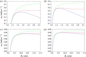
Figure 16 shows the angular speed
 $\unicode[STIX]{x1D714}_{0}$
of the steadily propagating surface in the arc geometry as a function of the outer radius
 $R_{e}$
for
 $R_{i}=1$
cm and
 $R_{i}=9$
cm for various confinement angles and for
 $D_{CJ}=0.78~\text{cm}~\unicode[STIX]{x03BC}\text{s}^{-1}$
and
 $B=0.1$
cm (as used in § 3). It compares a numerical solution for the steady solution determined by the method described in § 3 with the one-term approximation for
 $\unicode[STIX]{x1D714}_{0}~(=\unicode[STIX]{x1D714}_{00})$
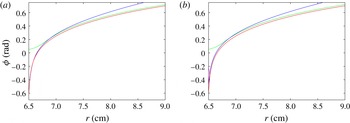
determined from (3.24) and the two-term approximation for
 $\unicode[STIX]{x1D714}_{0}$
given by (3.22b
) using (3.24) and (3.25). For reference, the size of
 $\unicode[STIX]{x1D716}$
for the two cases
 $R_{i}=1$
cm and
 $R_{i}=9$
cm can be estimated by making the choices
 $B_{ref}=B$
and
 $r_{ref}=R_{i}$
, giving
 $\unicode[STIX]{x1D716}=0.1$
for
 $R_{i}=1$
cm and
 $\unicode[STIX]{x1D716}=1/90$
for
 $R_{i}=9$
cm. In all cases, for sufficiently small
 $R_{e}$
, the numerical and two asymptotic solutions agree well. As
 $R_{e}$
increases, the one-term approximation
 $\unicode[STIX]{x1D714}\sim \unicode[STIX]{x1D714}_{00}$
diverges from the numerical solution, but the two-term approximation maintains good agreement with the numerical solution in the region where the approximation
 $\unicode[STIX]{x1D714}_{0}\sim \unicode[STIX]{x1D714}_{00}$
initially diverges, eventually diverging from the numerical solution as
 $R_{e}$
increases further. In all cases, the two-term approximation appears to break down when
 $\unicode[STIX]{x1D714}_{00}\rightarrow D_{CJ}/R_{i}$
(i.e.
 $0.78~\text{rad}~\unicode[STIX]{x03BC}\text{s}^{-1}$
for
 $R_{1}=1$
cm and
 $0.08666~\text{rad}~\unicode[STIX]{x03BC}\text{s}^{-1}$
for
 $R_{1}=9$
cm), and this appears to occur as
 $\unicode[STIX]{x1D714}_{0}$
for the numerical solution approaches a constant value for increasing
 $R_{e}$
. It is interesting to note, in the two cases shown for
 $R_{i}=9$
cm, the moderately large size of
 $R_{e}$
over which the two-term approximation to
 $\unicode[STIX]{x1D714}_{0}$
provides a reasonable approximation to the numerical solution, despite the small value of
 $\unicode[STIX]{x1D716}$
.
Surface normal angle variation as a function of
 $r$
with
 $\unicode[STIX]{x1D719}_{i}=-0.7$
,
 $\unicode[STIX]{x1D719}_{e}=0.7$
for (a)
 $R_{i}=1$
cm,
 $R_{e}=1.2$
cm, (b)
 $R_{i}=1$
cm,
 $R_{e}=1.4$
cm, (c)
 $R_{i}=9$
cm,
 $R_{e}=9.2$
cm and (d)
 $R_{i}=9$
cm,
 $R_{e}=10$
cm. A numerical solution (red) is shown against the two-term approximation
 $r\sim R_{i}(1+(B/R_{i})(\hat{r}_{1}/\hat{B}))$
(green) and the three-term approximation
 $r\sim R_{i}(1+(B/R_{i})(\hat{r}_{1}/\hat{B})+(B/R_{i})^{2}(\hat{r}_{2}\hat{R}_{i}/\hat{B}^{2}))$
(blue).

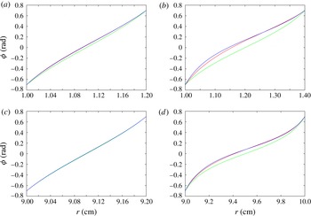
Figure 17 shows the surface normal angle variation with
 $r$
for
 $\unicode[STIX]{x1D719}_{i}=-0.7$
and
 $\unicode[STIX]{x1D719}_{e}=0.7$
for various choices of
 $R_{i}$
and
 $R_{e}$
, comparing a numerical solution against the two asymptotic approximations
 $r\sim R_{i}(1+(B/R_{i})(\hat{r}_{1}/\hat{B}))$
(calculated from (3.16)) and
 $r\sim R_{i}(1+(B/R_{i})(\hat{r}_{1}/\hat{B})+(B/R_{i})^{2}(\hat{r}_{2}\hat{R}_{i}/\hat{B}^{2}))$
(calculated from (3.16) and (3.23)). When
 $R_{i}=1$
cm and
 $R_{e}=1.2$
cm, the agreement between all three solutions is good. When
 $R_{i}=1$
cm and
 $R_{e}=1.4$
cm, the two-term approximation
 $r\sim R_{i}+B(\hat{r}_{1}/\hat{B})$
diverges from the numerical solution, but the three-term approximation provides a good agreement. Similarly, when
 $R_{i}=9$
cm and
 $R_{e}=9.2$
cm, the agreement between all three solutions is good. Even for
 $R_{e}=10$
cm, the three-term approximation for
 $r$
as a function of
 $\unicode[STIX]{x1D719}$
provides good agreement with the numerical solution.
3.2.2 Thicker arc case
As
 $\hat{R}_{e}$
gets larger, the thin arc asymptotics appear to run into difficulty as
 $\unicode[STIX]{x1D6FC}\rightarrow 1$
. We now consider the thicker arc case, defined by
 $\hat{R}_{e}-\hat{R}_{i}=O(1)$
, and make the ansatz (based on
 $\unicode[STIX]{x1D6FC}\sim 1$
) that
 $$\begin{eqnarray}\displaystyle \hat{\unicode[STIX]{x1D714}}_{0}\sim \frac{\hat{D}_{CJ}}{\hat{R}_{i}}. & & \displaystyle\end{eqnarray}$$
This implies that the leading-order surface angular speed is a function of
 $\hat{D}_{CJ}$
and the inner arc radius only. It corresponds to a Huygens limit (zero curvature) propagation model where
 $\hat{D}_{n}=\hat{D}_{CJ}$
assuming a constant angular velocity and perfect confinement on the inner arc surface
 $(\unicode[STIX]{x1D719}_{i}=0)$
. Then with
 $\hat{D}_{n}=\hat{\unicode[STIX]{x1D714}}_{0}\hat{r}\cos \unicode[STIX]{x1D719}$
, and assuming perfect confinement on
 $\hat{r}=\hat{R}_{i}$
, we have
 $\hat{D}_{CJ}=\hat{\unicode[STIX]{x1D714}}_{0}\hat{R}_{i}$
. This is simply the ansatz (3.27). The wave shape for this Huygens model limit is
 $\hat{r}=\hat{R}_{i}/\cos \unicode[STIX]{x1D719}$
. We show below that having the normal surface speed
 $\hat{D}_{n}$
depend on curvature
 $\hat{\unicode[STIX]{x1D705}}$
requires the insertion of a boundary layer structure near
 $\hat{r}=\hat{R}_{i}$
driven by increases in the magnitude of the surface wave curvature as
 $\hat{r}\rightarrow \hat{R}_{i}$
that are required to meet the enforced finite angle condition on
 $\hat{r}=\hat{R}_{i}$
. The changes in curvature in these layers determine the magnitude of the corrections to the leading-order angular speed (3.27). The solution away from
 $\hat{r}=\hat{R}_{i}$
corresponds, to leading order, to the Huygens limit propagation model.
We consider two cases of degree of inner arc confinement, denoted by weak confinement where
 $\unicode[STIX]{x1D719}_{i}=O(1)$
, and strong confinement where
 $\unicode[STIX]{x1D719}_{i}=O(\unicode[STIX]{x1D716}^{1/3})$
. For
 $\unicode[STIX]{x1D719}_{i}=O(1)$
, we show that the surface wave structure consists of a three-layer solution: there is an inner–inner layer, defined by
 $\hat{r}=\hat{R}_{i}+O(\unicode[STIX]{x1D716})$
, where
 $\unicode[STIX]{x1D719}=O(1)$
; an inner layer where
 $\hat{r}=\hat{R}_{i}+O(\unicode[STIX]{x1D716}^{2/3})$
, where
 $\unicode[STIX]{x1D719}=O(\unicode[STIX]{x1D716}^{1/3})$
; and an outer layer where
 $\hat{r}=O(1)$
and
 $\unicode[STIX]{x1D719}=O(1)$
. For the strong inner arc confinement case (
 $\unicode[STIX]{x1D719}_{i}=O(\unicode[STIX]{x1D716}^{1/3})$
), the inner–inner layer is not present and we find a two-layer structure with outer and inner layers defined by the same scalings just described. Our starting point is again (3.8). Below, we construct the surface wave structure layer by layer for the weak and strong inner arc confinement cases, and show that the angular wave speed
 $\hat{\unicode[STIX]{x1D714}}_{0}$
through
 $O(\unicode[STIX]{x1D716})$
is constructed by matching of the inner–inner and outer layers to the inner layer for
 $\unicode[STIX]{x1D719}_{i}=O(1)$
and matching of the inner to the outer layer for
 $\unicode[STIX]{x1D719}_{i}=O(\unicode[STIX]{x1D716}^{1/3})$
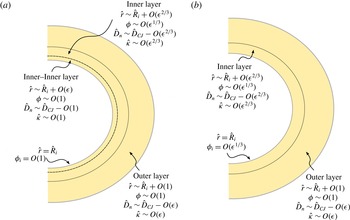
. A schematic of the various layers found in the analysis below for weak and strong inner arc confinement is shown in figure 18. In both cases, we expand the angular speed as
 $$\begin{eqnarray}\displaystyle \hat{\unicode[STIX]{x1D714}}_{0}\sim \hat{\unicode[STIX]{x1D714}}_{00}+\unicode[STIX]{x1D716}^{2/3}\hat{\unicode[STIX]{x1D714}}_{01}+\unicode[STIX]{x1D716}\hat{\unicode[STIX]{x1D714}}_{02},\quad & & \displaystyle\end{eqnarray}$$
where the appearance of the
 $O(\unicode[STIX]{x1D716}^{2/3})$
first correction term corresponds to the size of the curvature found in the inner layer solutions described below. Also,
 $$\begin{eqnarray}\displaystyle \hat{\unicode[STIX]{x1D714}}_{00}=\frac{\hat{D}_{CJ}}{\hat{R}_{i}} & & \displaystyle\end{eqnarray}$$
is consistent with the ansatz (3.27).
Surface wave layer structure for (a) inner arc weak confinement (
 $\unicode[STIX]{x1D719}_{i}=O(1)$
) and (b) inner arc strong confinement
 $\unicode[STIX]{x1D719}_{i}=O(\unicode[STIX]{x1D716}^{1/3})$
.

(i) Weak inner arc confinement
 $\unicode[STIX]{x1D719}_{i}=O(1)$
.
Outer layer: In the outer layer, characterized by
 $\hat{r}=O(1)$
and
 $\unicode[STIX]{x1D719}=O(1)$
, we define the expansions
 $$\begin{eqnarray}\displaystyle \hat{r}\sim \hat{r}_{0}+\unicode[STIX]{x1D716}^{2/3}\hat{r}_{1}+\unicode[STIX]{x1D716}\hat{r}_{2}, & & \displaystyle\end{eqnarray}$$
where the
 $O(\unicode[STIX]{x1D716}^{2/3})$
term arises due to (3.28). Substituting (3.30) and (3.28) into (3.8), we find that
 $$\begin{eqnarray}\displaystyle \left.\begin{array}{@{}c@{}}\displaystyle 1-\frac{\cos \unicode[STIX]{x1D719}}{\hat{D}_{CJ}}\hat{\unicode[STIX]{x1D714}}_{00}\hat{r}_{0}=0,\quad \hat{r}_{1}\hat{\unicode[STIX]{x1D714}}_{00}+\hat{r}_{0}\hat{\unicode[STIX]{x1D714}}_{01}=0,\\ \displaystyle \left(\frac{\cos \unicode[STIX]{x1D719}}{\hat{D}_{CJ}}(\hat{\unicode[STIX]{x1D714}}_{00}\hat{r}_{2}+\unicode[STIX]{x1D714}_{02}\hat{r}_{0})+\frac{\hat{B}\sin \unicode[STIX]{x1D719}}{\hat{r}_{0}}\right)\frac{\text{d}\hat{r}_{0}}{\text{d}\unicode[STIX]{x1D719}}=-\hat{B}\cos \unicode[STIX]{x1D719},\end{array}\right\} & & \displaystyle\end{eqnarray}$$
with solution
 $$\begin{eqnarray}\displaystyle \hat{r}_{0}=\frac{\hat{D}_{CJ}}{\hat{\unicode[STIX]{x1D714}}_{00}\cos \unicode[STIX]{x1D719}},\quad \hat{r}_{1}=-\frac{\hat{D}_{CJ}\hat{\unicode[STIX]{x1D714}}_{01}}{\hat{\unicode[STIX]{x1D714}}_{00}^{2}\cos \unicode[STIX]{x1D719}},\quad \hat{r}_{2}=-\frac{\hat{B}}{\sin \unicode[STIX]{x1D719}}-\frac{\hat{\unicode[STIX]{x1D714}}_{02}\hat{D}_{CJ}}{\hat{\unicode[STIX]{x1D714}}_{00}^{2}\cos \unicode[STIX]{x1D719}}. & & \displaystyle\end{eqnarray}$$
Note that, as
 $\unicode[STIX]{x1D719}\rightarrow \unicode[STIX]{x03C0}/2$
,
 $\hat{r}_{0}\rightarrow \infty$
. Assembling, we have that
 $$\begin{eqnarray}\displaystyle \hat{r}\sim \frac{\hat{D}_{CJ}}{\hat{\unicode[STIX]{x1D714}}_{00}\cos \unicode[STIX]{x1D719}}-\unicode[STIX]{x1D716}^{2/3}\frac{\hat{D}_{CJ}\hat{\unicode[STIX]{x1D714}}_{01}}{\hat{\unicode[STIX]{x1D714}}_{00}^{2}\cos \unicode[STIX]{x1D719}}-\unicode[STIX]{x1D716}\hat{B}\left(\frac{1}{\sin \unicode[STIX]{x1D719}}+\frac{\hat{\unicode[STIX]{x1D714}}_{02}\hat{D}_{CJ}}{\hat{B}\hat{\unicode[STIX]{x1D714}}_{00}^{2}\cos \unicode[STIX]{x1D719}}\right). & & \displaystyle\end{eqnarray}$$
The leading-order behaviour is the Huygens model solution described above. The corresponding expansions for
 $\hat{D}_{n}$
and
 $\hat{\unicode[STIX]{x1D705}}$
are given by
 $$\begin{eqnarray}\displaystyle \hat{D}_{n}=\hat{D}_{CJ}\left(1-\frac{\unicode[STIX]{x1D716}\hat{B}}{\hat{R}_{i}\tan \unicode[STIX]{x1D719}}\right),\quad \hat{\unicode[STIX]{x1D705}}=\frac{\unicode[STIX]{x1D716}}{\hat{R}_{i}\tan \unicode[STIX]{x1D719}}, & & \displaystyle\end{eqnarray}$$
so that both
 $\hat{\unicode[STIX]{x1D705}}$
and the variations of
 $\hat{D}_{n}$
from
 $\hat{D}_{CJ}$
are
 $O(\unicode[STIX]{x1D716})$
. As the surface normal angle
 $\unicode[STIX]{x1D719}\rightarrow 0$
, the first term in the
 $O(\unicode[STIX]{x1D716})$
expression in (3.33) becomes singular, while the magnitude of
 $\hat{\unicode[STIX]{x1D705}}$
increases beyond
 $O(\unicode[STIX]{x1D716})$
. This indicates that construction of an inner boundary layer in the region
 $\unicode[STIX]{x1D719}\sim 0$
is required.
Inner layer: A dominant balance argument leads to the conclusion that this layer appears near
 $\hat{r}=\hat{R}_{i}$
and requires construction of an inner layer near
 $\hat{r}=\hat{R}_{i}$
characterized by an
 $O(\unicode[STIX]{x1D716}^{1/3})$
variation in
 $\unicode[STIX]{x1D719}$
around
 $\unicode[STIX]{x1D719}=0$
, where
 $\hat{\unicode[STIX]{x1D705}}=O(\unicode[STIX]{x1D716}^{2/3})$
. We define a new variable
 $\tilde{\unicode[STIX]{x1D719}}$
such that
 $$\begin{eqnarray}\displaystyle \tilde{\unicode[STIX]{x1D719}}=\frac{\unicode[STIX]{x1D719}}{\unicode[STIX]{x1D716}^{1/3}}, & & \displaystyle\end{eqnarray}$$
with
 $$\begin{eqnarray}\displaystyle \hat{r}\sim \hat{R}_{i}+\unicode[STIX]{x1D716}^{2/3}\hat{r}_{1}+\unicode[STIX]{x1D716}\hat{r}_{2}. & & \displaystyle\end{eqnarray}$$
Substituting (3.36), (3.35) and (3.28) into (3.8), we obtain
 $$\begin{eqnarray}\displaystyle \left.\begin{array}{@{}c@{}}\displaystyle \frac{1}{\hat{D}_{CJ}}\left(\hat{\unicode[STIX]{x1D714}}_{01}\hat{R}_{i}+\hat{\unicode[STIX]{x1D714}}_{00}\hat{r}_{1}-\hat{\unicode[STIX]{x1D714}}_{00}\hat{R}_{i}\frac{\tilde{\unicode[STIX]{x1D719}}^{2}}{2}\right)\frac{\text{d}\hat{r}_{1}}{\text{d}\tilde{\unicode[STIX]{x1D719}}}=-\hat{B},\\ \displaystyle \left(\hat{\unicode[STIX]{x1D714}}_{01}\hat{R}_{i}+\hat{\unicode[STIX]{x1D714}}_{00}\hat{r}_{1}-\hat{\unicode[STIX]{x1D714}}_{00}\hat{R}_{i}\frac{\tilde{\unicode[STIX]{x1D719}}^{2}}{2}\right)\frac{\text{d}\hat{r}_{2}}{\text{d}\tilde{\unicode[STIX]{x1D719}}}+(\hat{\unicode[STIX]{x1D714}}_{02}\hat{R}_{i}+\hat{\unicode[STIX]{x1D714}}_{00}\hat{r}_{2})\frac{\text{d}\hat{r}_{1}}{\text{d}\tilde{\unicode[STIX]{x1D719}}}=0.\end{array}\right\} & & \displaystyle\end{eqnarray}$$
The equation for
 $\hat{r}_{1}$
can be written into a Ricatti equation form for
 $\tilde{\unicode[STIX]{x1D719}}$
, namely
 $$\begin{eqnarray}\displaystyle \left(\frac{\hat{\unicode[STIX]{x1D714}}_{01}}{\hat{\unicode[STIX]{x1D714}}_{00}}+\frac{\hat{r}_{1}}{\hat{R}_{i}}-\frac{\tilde{\unicode[STIX]{x1D719}}^{2}}{2}\right)=-\hat{B}\frac{\text{d}\tilde{\unicode[STIX]{x1D719}}}{\text{d}\hat{r}_{1}}, & & \displaystyle\end{eqnarray}$$
after using (3.29). This has the solution
 $$\begin{eqnarray}\displaystyle \left.\begin{array}{@{}c@{}}\displaystyle \tilde{\unicode[STIX]{x1D719}}=-2^{2/3}\left(\frac{\hat{B}}{\hat{R}_{i}}\right)^{1/3}\left[\frac{\text{Ai}^{\prime }(f(\hat{r}_{1}))+C_{1}\,\text{Bi}^{\prime }(f(\hat{r}_{1}))}{\text{Ai}(f(\hat{r}_{1}))+C_{1}\,\text{Bi}(f(\hat{r}_{1}))}\right],\\ \displaystyle f(\hat{r}_{1})=2^{-1/3}\left(\frac{\hat{B}}{\hat{R}_{i}}\right)^{-2/3}\left(\frac{\hat{r}_{1}}{\hat{R}_{i}}+\frac{\hat{\unicode[STIX]{x1D714}}_{01}}{\hat{\unicode[STIX]{x1D714}}_{00}}\right),\end{array}\right\} & & \displaystyle\end{eqnarray}$$
where
 $\text{Ai}$
and
 $\text{Bi}$
are the standard Airy functions and
 $C_{1}$
is an integration constant. Matching with the outer layer (as detailed in appendix A) requires
 $C_{1}=0$
. This leaves
 $$\begin{eqnarray}\displaystyle \tilde{\unicode[STIX]{x1D719}}=-2^{2/3}\left(\frac{\hat{B}}{\hat{R}_{i}}\right)^{1/3}\left[\frac{\text{Ai}^{\prime }(f(\hat{r}_{1}))}{\text{Ai}(f(\hat{r}_{1}))}\right]. & & \displaystyle\end{eqnarray}$$
Defining
 $\unicode[STIX]{x1D706}$
such that
 $$\begin{eqnarray}\displaystyle \frac{\text{Ai}^{\prime }(-\unicode[STIX]{x1D706})}{\text{Ai}(-\unicode[STIX]{x1D706})}=-2^{-2/3}\left(\frac{\hat{B}}{\hat{R}_{i}}\right)^{-1/3}\tilde{\unicode[STIX]{x1D719}}, & & \displaystyle\end{eqnarray}$$
then
 $\hat{r}_{1}$
can be written as
 $$\begin{eqnarray}\displaystyle \hat{r}_{1}=-\hat{R}_{i}\left(2^{1/3}\left(\frac{\hat{B}}{\hat{R}_{i}}\right)^{2/3}\unicode[STIX]{x1D706}+\frac{\hat{\unicode[STIX]{x1D714}}_{01}}{\hat{\unicode[STIX]{x1D714}}_{00}}\right). & & \displaystyle\end{eqnarray}$$
Using again (3.36), (3.35) and (3.28) in (3.8), the equation for
 $\hat{r}_{2}$
can be written as
 $$\begin{eqnarray}\displaystyle \frac{\text{d}\hat{r}_{2}}{\text{d}\tilde{\unicode[STIX]{x1D719}}}-\frac{\hat{B}}{\hat{R}_{i}g(\tilde{\unicode[STIX]{x1D719}})}\hat{r}_{2}=\frac{\hat{B}\hat{\unicode[STIX]{x1D714}}_{02}}{\hat{\unicode[STIX]{x1D714}}_{00}g(\tilde{\unicode[STIX]{x1D719}})},\quad g(\tilde{\unicode[STIX]{x1D719}})=\left(\frac{\hat{\unicode[STIX]{x1D714}}_{01}}{\hat{\unicode[STIX]{x1D714}}_{00}}+\frac{\hat{r}_{1}}{\hat{R}_{i}}-\frac{\tilde{\unicode[STIX]{x1D719}}^{2}}{2}\right)^{2}, & & \displaystyle\end{eqnarray}$$
with solution
 $$\begin{eqnarray}\displaystyle \hat{r}_{2}=-\hat{R}_{i}\frac{\hat{\unicode[STIX]{x1D714}}_{02}}{\hat{\unicode[STIX]{x1D714}}_{00}}+C_{2}\exp \left(\int ^{\tilde{\unicode[STIX]{x1D719}}}\frac{\hat{B}}{\hat{R}_{i}g(\tilde{\unicode[STIX]{x1D719}})}\,\text{d}\tilde{\unicode[STIX]{x1D719}}\right). & & \displaystyle\end{eqnarray}$$
Matching with the outer layer (appendix A) requires
 $C_{2}=0$
, whereupon
 $$\begin{eqnarray}\displaystyle \hat{r}_{2}=-\hat{R}_{i}\frac{\hat{\unicode[STIX]{x1D714}}_{02}}{\hat{\unicode[STIX]{x1D714}}_{00}}. & & \displaystyle\end{eqnarray}$$
The corresponding expansions for
 $\hat{D}_{n}$
and
 $\hat{\unicode[STIX]{x1D705}}$
are given by
 $$\begin{eqnarray}\displaystyle \left.\begin{array}{@{}c@{}}\displaystyle \hat{D}_{n}\sim \hat{D}_{CJ}\left[1-\unicode[STIX]{x1D716}^{2/3}\left[2^{1/3}\left(\frac{\hat{B}}{\hat{R}_{i}}\right)^{2/3}\unicode[STIX]{x1D706}+\frac{\tilde{\unicode[STIX]{x1D719}}^{2}}{2}\right]\right]+o(\unicode[STIX]{x1D716}),\\ \displaystyle \hat{\unicode[STIX]{x1D705}}\sim \unicode[STIX]{x1D716}^{2/3}\left[2^{1/3}\left(\frac{\hat{B}}{\hat{R}_{i}}\right)^{2/3}\frac{\unicode[STIX]{x1D706}}{\hat{B}}+\frac{\tilde{\unicode[STIX]{x1D719}}^{2}}{2\hat{B}}\right]+o(\unicode[STIX]{x1D716}).\end{array}\right\} & & \displaystyle\end{eqnarray}$$
The surface curvature in this layer is now
 $O(\unicode[STIX]{x1D716}^{2/3})$
, and it follows that deviations of
 $\hat{D}_{n}$
from
 $\hat{D}_{CJ}$
have increased to
 $O(\unicode[STIX]{x1D716}^{2/3})$
. However, since
 $\unicode[STIX]{x1D719}=O(\unicode[STIX]{x1D716}^{1/3})$
in this layer, the layer cannot extend all the way to the inner arc surface
 $(\hat{R}=\hat{R}_{i})$
where an
 $O(1)$
confinement angle is to be applied. Looking at the behaviour of (3.46) as
 $\tilde{\unicode[STIX]{x1D719}}\rightarrow -\infty$
, we see an additional layer is required at
 $\hat{r}=\hat{R}_{i}$
characterized by a further increase in the magnitude of the surface curvature.
Inner–inner layer: A dominant balance argument leads us to construct a boundary layer at
 $\hat{r}=\hat{R}_{i}$
where
 $\hat{r}=\hat{R}_{i}+O(\unicode[STIX]{x1D716})$
and
 $\unicode[STIX]{x1D719}=O(1)$
, and where
 $\hat{\unicode[STIX]{x1D705}}=O(1)$
. We define an expansion
 $$\begin{eqnarray}\displaystyle \hat{r}\sim \hat{R}_{i}+\unicode[STIX]{x1D716}\hat{r}_{1}+\unicode[STIX]{x1D716}^{5/3}\hat{r}_{2}, & & \displaystyle\end{eqnarray}$$
where, at
 $\hat{r}=\hat{R}_{i}$
,
 $\unicode[STIX]{x1D719}=\unicode[STIX]{x1D719}_{i}$
, and so
 $$\begin{eqnarray}\displaystyle \hat{r}_{1}(\unicode[STIX]{x1D719}_{i})=0,\quad \hat{r}_{2}(\unicode[STIX]{x1D719}_{i})=0. & & \displaystyle\end{eqnarray}$$
Substituting (3.47) and (3.28) into (3.8), we find
 $$\begin{eqnarray}\displaystyle (1-\cos \unicode[STIX]{x1D719})\frac{\text{d}\hat{r}_{1}}{\text{d}\unicode[STIX]{x1D719}}=\hat{B}\cos \unicode[STIX]{x1D719},\quad (1-\cos \unicode[STIX]{x1D719})\frac{\text{d}\hat{r}_{2}}{\text{d}\unicode[STIX]{x1D719}}=\frac{\hat{\unicode[STIX]{x1D714}}_{01}\hat{R}_{i}\cos \unicode[STIX]{x1D719}}{\hat{D}_{CJ}}\frac{\text{d}\hat{r}_{1}}{\text{d}\unicode[STIX]{x1D719}}, & & \displaystyle\end{eqnarray}$$
after making use of (3.29), with solution, subject to (3.48),
 $$\begin{eqnarray}\displaystyle \left.\begin{array}{@{}c@{}}\displaystyle \hat{r}_{1}=\hat{B}\left(-\frac{1}{\tan (\unicode[STIX]{x1D719}/2)}-\unicode[STIX]{x1D719}+\frac{1}{\tan (\unicode[STIX]{x1D719}_{i}/2)}+\unicode[STIX]{x1D719}_{i}\right),\\ \!\!\displaystyle \hat{r}_{2}=\frac{\hat{B}\hat{\unicode[STIX]{x1D714}}_{01}}{\hat{\unicode[STIX]{x1D714}}_{00}}\left(-\frac{1}{6\tan ^{3}(\unicode[STIX]{x1D719}/2)}+\frac{3}{2\tan (\unicode[STIX]{x1D719}/2)}+\unicode[STIX]{x1D719}+\frac{1}{6\tan ^{3}(\unicode[STIX]{x1D719}_{i}/2)}-\frac{3}{2\tan (\unicode[STIX]{x1D719}_{i}/2)}-\unicode[STIX]{x1D719}_{i}\right).\end{array}\right\} & & \displaystyle \nonumber\\ \displaystyle & & \displaystyle\end{eqnarray}$$
The corresponding expansions for
 $\hat{D}_{n}$
and
 $\hat{\unicode[STIX]{x1D705}}$
are given by
 $$\begin{eqnarray}\displaystyle \left.\begin{array}{@{}l@{}}\displaystyle \hat{D}_{n}\sim \hat{D}_{CJ}\left[\vphantom{\left[\left(\frac{\hat{B}}{\hat{R}_{i}}\right)\right]}\cos \unicode[STIX]{x1D719}-\unicode[STIX]{x1D716}^{2/3}\frac{(-\hat{\unicode[STIX]{x1D714}}_{01})}{\hat{\unicode[STIX]{x1D714}}_{00}}\cos \unicode[STIX]{x1D719}\right.\\ \displaystyle \left.\qquad +\,\unicode[STIX]{x1D716}\left[\frac{\hat{\unicode[STIX]{x1D714}}_{02}}{\hat{\unicode[STIX]{x1D714}}_{00}}\cos \unicode[STIX]{x1D719}+\left(\frac{\hat{B}}{\hat{R}_{i}}\right)\cos \unicode[STIX]{x1D719}\left(-\frac{1}{\tan (\unicode[STIX]{x1D719}/2)}-\unicode[STIX]{x1D719}+\frac{1}{\tan (\unicode[STIX]{x1D719}_{i}/2)}+\unicode[STIX]{x1D719}_{i}\right)\right]\right],\\ \displaystyle \hat{\unicode[STIX]{x1D705}}\sim \frac{1}{\hat{B}}\left[\vphantom{\left[\left(\frac{\hat{B}}{\hat{R}_{i}}\right)\right]}1-\cos \unicode[STIX]{x1D719}+\unicode[STIX]{x1D716}^{2/3}\frac{(-\hat{\unicode[STIX]{x1D714}}_{01})}{\hat{\unicode[STIX]{x1D714}}_{00}}\cos \unicode[STIX]{x1D719}\right.\\ \displaystyle \left.\qquad -\,\unicode[STIX]{x1D716}\left[\frac{\hat{\unicode[STIX]{x1D714}}_{02}}{\hat{\unicode[STIX]{x1D714}}_{00}}\cos \unicode[STIX]{x1D719}+\left(\frac{\hat{B}}{\hat{R}_{i}}\right)\cos \unicode[STIX]{x1D719}\left(-\frac{1}{\tan (\unicode[STIX]{x1D719}/2)}-\unicode[STIX]{x1D719}+\frac{1}{\tan (\unicode[STIX]{x1D719}_{i}/2)}+\unicode[STIX]{x1D719}_{i}\right)\right]\right].\end{array}\right\}\;\quad \; & & \displaystyle\end{eqnarray}$$
Thus in the inner–inner layer, both the surface curvature variations and the deviations of
 $\hat{D}_{n}$
from
 $\hat{D}_{CJ}$
are
 $O(1)$
.
Determination of the angular speed corrections: It now only remains to determine the angular speed corrections
 $\hat{\unicode[STIX]{x1D714}}_{01}$
and
 $\hat{\unicode[STIX]{x1D714}}_{02}$
. These are obtained by the matching process between the inner and inner–inner layer solutions. The specific details are given in appendix A. Matching of the inner and inner–inner solutions first requires
 $\text{Ai}(f(0))=0$
, or
 $$\begin{eqnarray}\displaystyle \text{Ai}\left(2^{-1/3}\left(\frac{\hat{B}}{\hat{R}_{i}}\right)^{-2/3}\frac{\hat{\unicode[STIX]{x1D714}}_{01}}{\hat{\unicode[STIX]{x1D714}}_{00}}\right)=0, & & \displaystyle\end{eqnarray}$$
which then defines
 $\hat{\unicode[STIX]{x1D714}}_{01}$
as
 $$\begin{eqnarray}\displaystyle \hat{\unicode[STIX]{x1D714}}_{01}=-2^{1/3}\unicode[STIX]{x1D707}\left(\frac{\hat{B}}{\hat{R}_{i}}\right)^{2/3}\hat{\unicode[STIX]{x1D714}}_{00}, & & \displaystyle\end{eqnarray}$$
where
 $\unicode[STIX]{x1D707}>0$
is the first positive value for which
 $\text{Ai}(-\unicode[STIX]{x1D707})=0$
, i.e.
 $\unicode[STIX]{x1D707}\approx 2.338107$
. Thus the
 $O(\unicode[STIX]{x1D716}^{2/3})$
first correction to the leading-order angular speed in (3.28) brings in a dependence on the
 $D_{n}$
–
 $\unicode[STIX]{x1D705}$
curvature scale parameter
 $\hat{B}$
, but does not, interestingly, depend on the degree of confinement on the inner arc. The correction term (3.53) is negative, so that the angular speed decreases when the normal surface velocity
 $\hat{D}_{n}$
depends on curvature. Similarly, the matching process between the inner–inner and inner layer solutions also gives the result for
 $\hat{\unicode[STIX]{x1D714}}_{02}$
, where
 $$\begin{eqnarray}\displaystyle \hat{\unicode[STIX]{x1D714}}_{02}=-\frac{\hat{B}\hat{D}_{CJ}}{\hat{R}_{i}^{2}}\left(\frac{1}{\tan (\unicode[STIX]{x1D719}_{i}/2)}+\unicode[STIX]{x1D719}_{i}\right). & & \displaystyle\end{eqnarray}$$
Given
 $\unicode[STIX]{x1D719}_{i}<0$
, then
 $\hat{\unicode[STIX]{x1D714}}_{02}>0$
. Thus for weak confinement, where
 $\unicode[STIX]{x1D719}_{i}=O(1)$
, the influence of the inner arc confinement on the angular surface speed
 $\hat{\unicode[STIX]{x1D714}}_{0}$
is found to enter in the
 $O(\unicode[STIX]{x1D716})$
correction term.
(ii) Strong inner arc confinement
 $\unicode[STIX]{x1D719}_{i}=O(\unicode[STIX]{x1D716}^{1/3})$
.
For
 $\unicode[STIX]{x1D719}_{i}=O(1)$
, we have identified a three-layer structure to the surface wave variation across the arc. We now consider a situation of strong confinement on the inner arc given by
 $\unicode[STIX]{x1D719}_{i}=O(\unicode[STIX]{x1D716}^{1/3})$
. In this case, the surface wave variation has a two-layer structure. It consists of an unmodified form of the outer layer solution described above, with a modified inner layer solution that now extends formally to
 $\hat{r}=\hat{R}_{i}$
. The inner layer solutions to (3.37) retaining the consequences of matching with the outer layer solution (3.33) are
 $$\begin{eqnarray}\displaystyle \tilde{\unicode[STIX]{x1D719}}=-2^{2/3}\left(\frac{\hat{B}}{\hat{R}_{i}}\right)^{1/3}\left[\frac{\text{Ai}^{\prime }(f(\hat{r}_{1}))}{\text{Ai}(f(\hat{r}_{1}))}\right],\quad \hat{r}_{2}=-\frac{\hat{R}_{i}\hat{\unicode[STIX]{x1D714}}_{02}}{\hat{\unicode[STIX]{x1D714}}_{00}}, & & \displaystyle\end{eqnarray}$$
where
 $f(\hat{r}_{1})$
is given by the second of equations (3.39). Rather than matching with the inner–inner layer, these are now subject to the conditions
 $\unicode[STIX]{x1D719}=\unicode[STIX]{x1D716}^{1/3}\tilde{\unicode[STIX]{x1D719}}_{i}$
on
 $\hat{r}=\hat{R}_{i}$
, whereupon
 $$\begin{eqnarray}\displaystyle \hat{r}_{1}(\tilde{\unicode[STIX]{x1D719}}_{i})=0,\quad \hat{r}_{2}(\tilde{\unicode[STIX]{x1D719}}_{i})=0. & & \displaystyle\end{eqnarray}$$
The first boundary condition gives an equation for
 $\hat{\unicode[STIX]{x1D714}}_{01}$
, namely
 $$\begin{eqnarray}\displaystyle \hat{\unicode[STIX]{x1D714}}_{01}=-2^{1/3}\unicode[STIX]{x1D708}\left(\frac{\hat{B}}{\hat{R}_{i}}\right)^{2/3}\frac{\hat{D}_{CJ}}{\hat{R}_{i}}, & & \displaystyle\end{eqnarray}$$
where
 $\unicode[STIX]{x1D708}>0$
is the first positive zero of the equation
 $$\begin{eqnarray}\displaystyle \frac{\text{Ai}^{\prime }(-\unicode[STIX]{x1D708})}{\text{Ai}(-\unicode[STIX]{x1D708})}=-2^{-2/3}\left(\frac{\hat{B}}{\hat{R}_{i}}\right)^{-1/3}\tilde{\unicode[STIX]{x1D719}}_{i}. & & \displaystyle\end{eqnarray}$$
Similarly, the condition on
 $\hat{r}_{2}$
implies that
 $$\begin{eqnarray}\displaystyle \hat{\unicode[STIX]{x1D714}}_{02}=0. & & \displaystyle\end{eqnarray}$$
Thus for strong confinement on the inner arc, where
 $\unicode[STIX]{x1D719}_{i}=O(\unicode[STIX]{x1D716}^{1/3})$
, the effects of confinement on the surface angular speed are now promoted to the
 $O(\unicode[STIX]{x1D716}^{2/3})$
correction term, where the effect of curvature also first appears. Using (3.57) and (3.59), we have, in the inner layer,
 $$\begin{eqnarray}\displaystyle \hat{r}_{1}=-\hat{R}_{i}2^{1/3}\left(\frac{\hat{B}}{\hat{R}_{i}}\right)^{2/3}(\unicode[STIX]{x1D706}-\unicode[STIX]{x1D708}),\quad \hat{r}_{2}=0. & & \displaystyle\end{eqnarray}$$
The expressions for
 $\hat{D}_{n}$
and
 $\hat{\unicode[STIX]{x1D705}}$
in the outer and inner layers are the same as (3.34) and (3.46).
The strong confinement case
 $\unicode[STIX]{x1D719}_{i}=O(\unicode[STIX]{x1D716}^{1/3})$
also contains as a subcase the perfect confinement limit
 $\unicode[STIX]{x1D719}_{i}=0$
that would be applicable to gas detonation propagation in a curved channel (Nakayama et al.
Reference Nakayama, Moriya, Kasahara, Matsuo, Sasamoto and Funaki2012, Reference Nakayama, Kasahara, Matsuo and Funaki2013). Here, the angular speed correction
 $\hat{\unicode[STIX]{x1D714}}_{01}$
is again given by (3.57), but where
 $\unicode[STIX]{x1D708}$
is now determined by
 $$\begin{eqnarray}\displaystyle \text{Ai}^{\prime }(-\unicode[STIX]{x1D708})=0,\quad \unicode[STIX]{x1D708}\approx 1.018793. & & \displaystyle\end{eqnarray}$$
Thus even with perfect confinement, a dependence of the normal surface speed
 $\hat{D}_{n}$
on curvature
 $\hat{\unicode[STIX]{x1D705}}$
requires the insertion of a boundary layer at the inner arc surface characterized by
 $\unicode[STIX]{x1D719}=O(\unicode[STIX]{x1D716}^{1/3})$
to account for the increase in curvature required to meet the perfect confinement conditions on
 $\hat{r}=\hat{R}_{i}$
.
Note that it is also possible to consider inner arc confinement angles between
 $\unicode[STIX]{x1D719}_{i}=O(1)$
and
 $\unicode[STIX]{x1D719}_{i}=O(\unicode[STIX]{x1D716}^{1/3})$
. Specifically, assuming a confinement angle
 $\unicode[STIX]{x1D719}_{i}=\unicode[STIX]{x1D716}^{\unicode[STIX]{x1D6FF}}\tilde{\unicode[STIX]{x1D719}}_{i}$
, where
 $0<\unicode[STIX]{x1D6FF}<1/3$
, a three-layer structure is again found, where now
 $$\begin{eqnarray}\displaystyle \hat{\unicode[STIX]{x1D714}}_{0}\sim \hat{\unicode[STIX]{x1D714}}_{00}+\unicode[STIX]{x1D716}^{2/3}\hat{\unicode[STIX]{x1D714}}_{01}+\unicode[STIX]{x1D716}^{1-\unicode[STIX]{x1D6FF}}\hat{\unicode[STIX]{x1D714}}_{02}. & & \displaystyle\end{eqnarray}$$
Minor modifications to the
 $\unicode[STIX]{x1D719}_{i}=O(1)$
analysis described above are required. In the outer layer, the surface normal angle scale remains
 $\unicode[STIX]{x1D719}=O(1)$
, while the inner layer angle scale also remains
 $\unicode[STIX]{x1D719}=O(\unicode[STIX]{x1D716}^{1/3})$
. The original
 $O(\unicode[STIX]{x1D716})$
perturbation term to
 $\hat{r}$
in these layers now becomes an
 $O(\unicode[STIX]{x1D716}^{1-\unicode[STIX]{x1D6FF}})$
perturbation term. In the inner–inner layer, the angle scale is now
 $\unicode[STIX]{x1D719}=O(\unicode[STIX]{x1D716}^{1-\unicode[STIX]{x1D6FF}})$
, where the first perturbation to the leading-order solution
 $\hat{r}=\hat{R}_{i}$
is
 $O(\unicode[STIX]{x1D716}^{1-\unicode[STIX]{x1D6FF}})$
. It is found that
 $\hat{\unicode[STIX]{x1D714}}_{01}$
remains unchanged from (3.53), but
 $\hat{\unicode[STIX]{x1D714}}_{02}$
is now given by
 $$\begin{eqnarray}\displaystyle \hat{\unicode[STIX]{x1D714}}_{02}=-\frac{2\hat{B}}{\tilde{\unicode[STIX]{x1D719}}_{i}}\frac{\hat{D}_{CJ}}{\hat{R}_{i}^{2}}. & & \displaystyle\end{eqnarray}$$
This result is consistent with the
 $\unicode[STIX]{x1D719}_{i}=O(1)$
expression for
 $\hat{\unicode[STIX]{x1D714}}_{02}$
(3.54) taking
 $\unicode[STIX]{x1D719}_{i}=O(\unicode[STIX]{x1D716}^{\unicode[STIX]{x1D6FF}})$
. We do not consider this confinement range further in the current article.
(iii) Boundary layer analysis for a specified angle condition on
 $r=R_{e}$
.
To determine the angular speed corrections to the leading-order Huygens propagation limit result (3.29) through
 $O(\unicode[STIX]{x1D716})$
, we have not had to make any specification either of the location of the outer arc boundary
 $\hat{r}=\hat{R}_{e}$
or the angle condition
 $\unicode[STIX]{x1D719}=\unicode[STIX]{x1D719}_{e}$
on
 $\hat{r}=\hat{R}_{e}$
. Rather, these corrections result from the changes in surface curvature in the boundary layer(s) near
 $\hat{r}=\hat{R}_{i}$
required to enforce the angle condition
 $\unicode[STIX]{x1D719}=\unicode[STIX]{x1D719}_{i}$
at the inner arc
 $\hat{r}=\hat{R}_{i}$
. This behaviour is consistent with the numerical results described in § 3.1. Nevertheless, we can invert (3.33) to find the normal surface angle
 $(\unicode[STIX]{x1D719}=\unicode[STIX]{x1D719}_{o})$
on
 $\hat{r}=\hat{R}_{e}$
determined by the outer layer solution, whereby
 $$\begin{eqnarray}\displaystyle \unicode[STIX]{x1D719}_{o}\sim \cos ^{-1}\left(\frac{\hat{R}_{i}}{\hat{R}_{e}}\right)+\unicode[STIX]{x1D716}^{2/3}\frac{\hat{\unicode[STIX]{x1D714}}_{01}}{\hat{\unicode[STIX]{x1D714}}_{00}}\frac{\hat{R}_{i}}{\sqrt{\hat{R}_{e}^{2}-\hat{R}_{i}^{2}}}+\unicode[STIX]{x1D716}\frac{\hat{R}_{i}}{\sqrt{\hat{R}_{e}^{2}-\hat{R}_{i}^{2}}}\left(\frac{\hat{B}}{\sqrt{\hat{R}_{e}^{2}-\hat{R}_{i}^{2}}}+\frac{\hat{\unicode[STIX]{x1D714}}_{02}}{\hat{\unicode[STIX]{x1D714}}_{00}}\right).\quad & & \displaystyle\end{eqnarray}$$
Generally, an enforced angle condition
 $\unicode[STIX]{x1D719}=\unicode[STIX]{x1D719}_{e}$
on
 $\hat{r}=\hat{R}_{e}$
would not be equal to
 $\unicode[STIX]{x1D719}_{o}$
(typically
 $\unicode[STIX]{x1D719}_{e}<\unicode[STIX]{x1D719}_{o}$
). Consequently, in order to enforce a boundary angle at
 $\hat{r}=\hat{R}_{e}$
, a boundary layer structure must be inserted at
 $\hat{r}=\hat{R}_{e}$
. It must be consistent with the already determined angular speed
 $\hat{\unicode[STIX]{x1D714}}_{0}$
and connect the angle (3.64) determined by the outer layer solution to the specified angle
 $\unicode[STIX]{x1D719}=\unicode[STIX]{x1D719}_{e}$
at
 $\hat{r}=\hat{R}_{e}$
. The details of such a boundary layer analysis are given in appendix C for the most complex case where
 $\unicode[STIX]{x1D719}_{o}-\unicode[STIX]{x1D719}_{e}=O(1)$
. It actually consists of a two-layer structure, one layer of size
 $O(\unicode[STIX]{x1D716})$
at
 $\hat{r}=\hat{R}_{e}$
in which
 $\unicode[STIX]{x1D719}=O(1)$
, and a second layer further in from
 $\hat{r}=\hat{R}_{e}$
, where
 $\hat{r}=\hat{R}_{e}+C_{r}\unicode[STIX]{x1D716}\ln \unicode[STIX]{x1D716}+O(\unicode[STIX]{x1D716})$
, in which variations about the strained
 $\unicode[STIX]{x1D719}$
coordinate location
 $$\begin{eqnarray}\displaystyle \unicode[STIX]{x1D719}=\cos ^{-1}\left(\frac{\hat{R}_{i}}{\hat{R}_{e}}\right)+\unicode[STIX]{x1D716}^{2/3}\frac{\hat{\unicode[STIX]{x1D714}}_{01}}{\hat{\unicode[STIX]{x1D714}}_{00}}\frac{\hat{R}_{i}}{\sqrt{\hat{R}_{e}^{2}-\hat{R}_{i}^{2}}}+C_{\unicode[STIX]{x1D719}}\unicode[STIX]{x1D716}\ln \unicode[STIX]{x1D716} & & \displaystyle\end{eqnarray}$$
are also
 $O(\unicode[STIX]{x1D716})$
. In total, an
 $O(1)$
imposed angle condition on both
 $\hat{r}=\hat{R}_{i}$
and
 $\hat{r}=\hat{R}_{e}$
(with
 $\unicode[STIX]{x1D719}_{o}-\unicode[STIX]{x1D719}_{e}=O(1)$
) would require the presence of five layers connecting
 $\hat{r}=\hat{R}_{i}$
to
 $\hat{r}=\hat{R}_{e}$
. The boundary layer structure for
 $\unicode[STIX]{x1D719}_{o}-\unicode[STIX]{x1D719}_{e}=o(1)$
can be more easily described and is left as an exercise for the interested reader. The general need to insert a boundary layer at
 $\hat{r}=\hat{R}_{e}$
to enforce an angle condition on
 $\hat{r}=\hat{R}_{e}$
that does not influence the angular speed provides support for use of a continuation condition at the outer arc surface for thick arcs as described in § 3.1. For the asymptotic solution, the angle
 $\unicode[STIX]{x1D719}=\unicode[STIX]{x1D719}_{o}$
would then arise at
 $\hat{r}=\hat{R}_{e}$
.
(iv) Discussion of angular speed variation.
We now summarize the above results for the surface angular speed. For
 $\unicode[STIX]{x1D719}_{i}=O(1)$
,
 $$\begin{eqnarray}\displaystyle \hat{\unicode[STIX]{x1D714}}_{0}\sim \frac{\hat{D}_{CJ}}{\hat{R}_{i}}\left(1-\unicode[STIX]{x1D716}^{2/3}\left[2^{1/3}\unicode[STIX]{x1D707}\left(\frac{\hat{B}}{\hat{R}_{i}}\right)^{2/3}\right]+\unicode[STIX]{x1D716}\left[\frac{\hat{B}}{\hat{R}_{i}}\left(-\frac{1}{\tan (\unicode[STIX]{x1D719}_{i}/2)}-\unicode[STIX]{x1D719}_{i}\right)\right]\right), & & \displaystyle\end{eqnarray}$$
in scaled variables, or, equivalently,
 $$\begin{eqnarray}\displaystyle \unicode[STIX]{x1D714}_{0}\sim \frac{D_{CJ}}{R_{i}}\left(1-2^{1/3}\unicode[STIX]{x1D707}\left(\frac{B}{R_{i}}\right)^{2/3}+\frac{B}{R_{i}}\left(-\frac{1}{\tan (\unicode[STIX]{x1D719}_{i}/2)}-\unicode[STIX]{x1D719}_{i}\right)\right), & & \displaystyle\end{eqnarray}$$
in unscaled form, where
 $\text{Ai}(-\unicode[STIX]{x1D707})=0$
, i.e.
 $\unicode[STIX]{x1D707}\approx 2.338107$
. Thus to leading order, the angular speed is determined by the linear speed of the CJ detonation relative to the magnitude of the inner radius of the arc. As noted above, it corresponds to a Huygens limit propagation model (where
 $D_{n}=D_{CJ}$
), assuming perfect confinement on the inner arc surface. At the next order
 $O((B/R_{i})^{2/3})$
, defined by the size of the ratio
 $B/R_{i}$
, the effects of normal surface speed variability with curvature now enter. Then at
 $O(B/R_{i})$
, the effects of confinement on the inner arc appear. To this order, neither the magnitude of the outer radius nor the magnitude of the confinement on the outer arc affect the angular speed. For
 $\unicode[STIX]{x1D719}_{i}=O(\unicode[STIX]{x1D716}^{1/3})$
, we have,
 $$\begin{eqnarray}\displaystyle \hat{\unicode[STIX]{x1D714}}_{0}\sim \frac{\hat{D}_{CJ}}{\hat{R}_{i}}\left(1-\unicode[STIX]{x1D716}^{2/3}\left[2^{1/3}\unicode[STIX]{x1D708}\left(\frac{\hat{B}}{\hat{R}_{i}}\right)^{2/3}\right]\right), & & \displaystyle\end{eqnarray}$$
in scaled variables, or, equivalently,
 $$\begin{eqnarray}\displaystyle \unicode[STIX]{x1D714}_{0}\sim \frac{D_{CJ}}{R_{i}}\left(1-2^{1/3}\unicode[STIX]{x1D708}\left(\frac{B}{R_{i}}\right)^{2/3}\right), & & \displaystyle\end{eqnarray}$$
in unscaled form, where
 $\unicode[STIX]{x1D708}$
is determined by the first zero of
 $$\begin{eqnarray}\displaystyle \frac{\text{Ai}^{\prime }(-\unicode[STIX]{x1D708})}{\text{Ai}(-\unicode[STIX]{x1D708})}=-2^{-2/3}\left(\frac{B}{R_{i}}\right)^{-1/3}\unicode[STIX]{x1D719}_{i}. & & \displaystyle\end{eqnarray}$$
Thus to leading order,
 $\unicode[STIX]{x1D714}_{0}$
again depends only on
 $D_{CJ}$
and
 $R_{i}$
, while the effects of curvature and inner arc confinement now both appear in the first correction term at
 $O((B/R_{i})^{2/3})$
. When
 $\unicode[STIX]{x1D719}_{i}=0$
,
 $\unicode[STIX]{x1D708}$
is given by
 $\text{Ai}^{\prime }(-\unicode[STIX]{x1D708})=0$
, i.e.
 $\unicode[STIX]{x1D708}\approx 1.018793$
.
These asymptotic results above go some way to explaining the observed behaviour of the variation of
 $\unicode[STIX]{x1D714}_{0}$
with
 $R_{e}$
seen in figure 5, where, for sufficiently thick arcs, the angular speed becomes independent of the outer arc radius or confinement, and where the angular speed dependence on the inner arc confinement is moderately weak.
(a) Comparison of the one-term (green), two-term (magenta) and three-term (blue) approximations to the angular speed
 $\unicode[STIX]{x1D714}_{0}$
for weak inner arc confinement (from (3.67)) as a function of inner arc radius
 $R_{i}$
for
 $\unicode[STIX]{x1D719}_{i}=-0.7$
. The values
 $D_{CJ}=0.78~\text{cm}~\unicode[STIX]{x03BC}\text{s}^{-1}$
and
 $B=0.1$
cm are used. Also shown is a numerical solution (red) for thick arcs, specifically where
 $R_{e}=R_{i}+5$
cm and
 $\unicode[STIX]{x1D719}_{e}=0.7$
. (b) As for (a), but now comparing the linear speed
 $R_{i}\unicode[STIX]{x1D714}_{0}$
on the inner arc.

Figure 19 shows a comparison of the one-term, two-term and three-term approximations to the angular speed
 $\unicode[STIX]{x1D714}_{0}$
and the linear speed
 $R_{i}\unicode[STIX]{x1D714}_{0}$
for the weak inner arc confinement result (3.67) as a function of inner arc radius
 $R_{i}$
. The inner arc confinement angle was taken to be
 $\unicode[STIX]{x1D719}_{i}=-0.7$
, and, as in § 3.1, the values
 $D_{CJ}=0.78~\text{cm}~\unicode[STIX]{x03BC}\text{s}^{-1}$
and
 $B=0.1$
cm are used. The linear speed
 $R_{i}\unicode[STIX]{x1D714}_{0}$
on the inner arc is used to amplify differences in
 $\unicode[STIX]{x1D714}_{0}$
for large
 $R_{i}$
. These are compared to a corresponding numerical solution for sufficiently thick arcs where
 $\unicode[STIX]{x1D714}_{0}$
is essentially independent of
 $R_{e}$
and
 $\unicode[STIX]{x1D719}_{e}$
as described in § 3.1. The three-term approximation to
 $\unicode[STIX]{x1D714}_{0}$
provides a good approximation except for the smaller values of
 $R_{i}$
, with the approximation improving as
 $R_{i}$
increases. If we make the choices
 $B_{ref}=B$
and
 $r_{ref}=R_{i}$
, then the improvement in the approximation as
 $R_{i}$
increases corresponds to a decrease in the value of
 $\unicode[STIX]{x1D716}=B/R_{i}$
. In figure 19 we have compared the variation in
 $\unicode[STIX]{x1D714}_{0}$
with
 $R_{i}$
for a confinement angle
 $\unicode[STIX]{x1D719}_{i}=-0.7$
using the weak inner arc confinement result (3.67), but it is not clear at which values of
 $\unicode[STIX]{x1D719}_{i}$
the weak or strong confinement solutions (3.67) and (3.69) will provide a better approximation. Figure 20 shows a comparison of the two-term approximation from the strong inner arc confinement solution (3.69) to the linear speed
 $R_{i}\unicode[STIX]{x1D714}_{0}$
with both the three-term (blue) approximation from the weak inner arc confinement solution (3.67) and the numerical solution shown in figure 19(b). Clearly, for the choice
 $\unicode[STIX]{x1D719}_{i}=-0.7$
(with
 $D_{CJ}=0.78~\text{cm}~\unicode[STIX]{x03BC}\text{s}^{-1}$
and
 $B=0.1$
cm), the three-term weak confinement solution provides a better approximation to the numerical solution, although, for large
 $R_{i}$
, the two-term strong inner arc confinement solution also provides a good approximation.
Comparison corresponding to figure 19 of the three-term (blue) approximation to the linear speed
 $R_{i}\unicode[STIX]{x1D714}_{0}$
from the weak inner arc confinement solution (3.67) with the two-term (green) approximation from the strong inner arc confinement solution (3.69) and a numerical solution (red).

Figure 21 shows a comparison of the one-term and two-term approximation to the angular speed
 $\unicode[STIX]{x1D714}_{0}$
and the linear speed
 $R_{i}\unicode[STIX]{x1D714}_{0}$
for the strong inner arc confinement result (3.69) as a function of inner arc radius
 $R_{i}$
. The inner arc confinement angle was taken to be
 $\unicode[STIX]{x1D719}_{i}=-0.2$
. Again, the values
 $D_{CJ}=0.78~\text{cm}~\unicode[STIX]{x03BC}\text{s}^{-1}$
and
 $B=0.1$
cm are used. These are compared to a corresponding numerical solution for sufficiently thick arcs. The two-term approximation to
 $\unicode[STIX]{x1D714}_{0}$
provides a good approximation except for the smaller values of
 $R_{i}$
, with again the approximation improving as
 $R_{i}$
increases. Figure 22 shows a comparison of the three-term approximation to the linear speed
 $R_{i}\unicode[STIX]{x1D714}_{0}$
from the weak inner arc confinement solution (3.67) with both the two-term approximation from the strong inner arc confinement solution (3.69) and the numerical solution shown in figure 21. Clearly, for the small confinement angle
 $\unicode[STIX]{x1D719}_{i}=-0.2$
, the three-term weak confinement solution (3.67) does not provide a reasonable approximation.
(a) Comparison of the one-term (green) and two-term (blue) approximations to the angular speed
 $\unicode[STIX]{x1D714}_{0}$
for strong inner arc confinement (from (3.69)) as a function of inner arc radius
 $R_{i}$
for
 $\unicode[STIX]{x1D719}_{i}=-0.2$
. The values
 $D_{CJ}=0.78~\text{cm}~\unicode[STIX]{x03BC}\text{s}^{-1}$
and
 $B=0.1$
cm are used. Also shown is a numerical solution (red) for thick arcs, specifically where
 $R_{e}=R_{i}+5$
cm and
 $\unicode[STIX]{x1D719}_{e}=0.7$
. (b) As for (a), but now comparing the linear speed
 $R_{i}\unicode[STIX]{x1D714}_{0}$
.

Comparison corresponding to figure 21 of the three-term (blue) approximation to the linear speed
 $R_{i}\unicode[STIX]{x1D714}_{0}$
from the weak inner arc confinement solution (3.67) with the two-term (green) approximation from the strong inner arc confinement solution (3.69) and a numerical solution (red).

(v) Variation of
 $r$
,
 $D_{n}$
and
 $\unicode[STIX]{x1D705}$
with
 $\unicode[STIX]{x1D719}$
.
Appendix B gives the variation of
 $r$
,
 $D_{n}$
and
 $\unicode[STIX]{x1D705}$
with
 $\unicode[STIX]{x1D719}$
in unscaled form for the weak and strong inner arc confinement cases above. The asymptotic results for
 $D_{n}$
and
 $\unicode[STIX]{x1D705}$
shed light on the behaviour observed in § 3.1, and show that both the variations in
 $D_{n}$
from
 $D_{CJ}$
and those in
 $\unicode[STIX]{x1D705}$
are associated with a multi-layer solution to the surface wave structure across the arc. Note that we have found it difficult to write down suitably well-behaved composite solutions for the layer-by-layer expressions in appendix B valid across all layers. This occurs for a number of reasons, such as the difficulty with constructing composite solutions across three layers, as well as the appearance of switchbacking terms in the intermediate matching regimes described in appendix A.
Surface normal angle variation as a function of
 $r$
for
 $D_{CJ}=0.78~\text{cm}~\unicode[STIX]{x03BC}\text{s}^{-1}$
,
 $B=0.1$
cm and
 $R_{i}\leqslant r\leqslant R_{e}$
, with
 $\unicode[STIX]{x1D719}_{i}=-0.2$
and (a)
 $R_{i}=1$
cm,
 $R_{e}=2.8$
cm and (b)
 $R_{i}=9$
cm,
 $R_{e}=13.75$
cm. Shown are the inner (blue) and outer (green) asymptotic solutions from the strong confinement results (B 5) and (B 6), as well as a numerical solution (red) based on a continuation solution at
 $r=R_{e}$
.

Surface normal angle variation as a function of
 $r$
for
 $D_{CJ}=0.78~\text{cm}~\unicode[STIX]{x03BC}\text{s}^{-1}$
,
 $B=0.1$
cm and
 $R_{i}\leqslant r\leqslant R_{e}$
, with
 $\unicode[STIX]{x1D719}_{i}=-0.7$
,
 $R_{i}=9$
cm and
 $R_{e}=13.75$
cm. Shown in (a) are the inner–inner (magenta), inner (blue) and outer (green) asymptotic solutions from the weak confinement results (B 1), (B 2) and (B 4), as well as a numerical solution (red) based on a continuation solution at
 $r=R_{e}$
. Shown in (b) are the inner (blue) and outer (green) asymptotic solutions from the strong confinement results (B 5) and (B 6), as well as the numerical solution (red) based on a continuation solution at
 $r=R_{e}$
.

Surface normal angle variation as a function of
 $r$
for
 $D_{CJ}=0.78~\text{cm}~\unicode[STIX]{x03BC}\text{s}^{-1}$
,
 $B=0.1$
cm and
 $R_{i}\leqslant r\leqslant R_{e}$
, with
 $\unicode[STIX]{x1D719}_{i}=-0.7$
,
 $R_{i}=1$
cm and
 $R_{e}=2.8$
cm. Shown in (a) are the inner–inner (magenta), inner (blue) and outer (green) asymptotic solutions from the weak confinement results (B 1), (B 2) and (B 4), as well as a numerical solution (red) based on a continuation solution at
 $r=R_{e}$
. Shown in (b) are the inner (blue) and outer (green) asymptotic solutions from the strong confinement results (B 5) and (B 6), as well as the numerical solution (red) based on a continuation solution at
 $r=R_{e}$
.

Figure 23 shows the surface normal angle variation as a function of
 $r$
for
 $\unicode[STIX]{x1D719}_{i}=-0.2$
, comparing the inner and outer asymptotic solutions from the strong confinement analysis (B 5) and (B 6) with a numerical solution. This is for
 $D_{CJ}=0.78~\text{cm}~\unicode[STIX]{x03BC}\text{s}^{-1}$
,
 $B=0.1$
cm and
 $R_{i}\leqslant r\leqslant R_{e}$
, with in one case,
 $R_{i}=1$
cm,
 $R_{e}=2.8$
cm, and in the other
 $R_{i}=9$
cm,
 $R_{e}=13.75$
cm. In both cases, good agreement with the numerical solution is found and provides a good representation of where the solutions in the inner and outer layers are active. Figure 24 shows the surface normal angle variation as a function of
 $r$
for
 $\unicode[STIX]{x1D719}_{i}=-0.7$
, comparing the inner–inner, inner and outer asymptotic solutions from the weak confinement results (B 1), (B 2) and (B 4) with that from the inner and outer asymptotic solutions from the strong confinement results (B 5) and (B 6), and with a numerical solution. Again, this is for
 $D_{CJ}=0.78~\text{cm}~\unicode[STIX]{x03BC}\text{s}^{-1}$
,
 $B=0.1$
cm and
 $R_{i}\leqslant r\leqslant R_{e}$
, with
 $R_{i}=9$
cm and
 $R_{e}=13.75$
cm. Both the strong and weak confinement asymptotic solutions are reasonable. It is interesting to note, however, that, despite the comparatively poorer agreement of the angular speed
 $\unicode[STIX]{x1D714}_{0}$
for the strong confinement solution compared to the weak confinement solution (see figure 20), the variation of
 $r$
with
 $\unicode[STIX]{x1D719}$
appears to be better captured by the strong confinement solution, particularly near to
 $r=R_{i}$
. This is probably influenced by the lack of construction of a reasonable composite solution. Figure 25 shows the surface normal angle variation as a function of
 $r$
, again for
 $\unicode[STIX]{x1D719}_{i}=-0.7$
, comparing the inner–inner, inner and outer asymptotic solutions from the weak confinement results (B 1), (B 2) and (B 4) with that from the inner and outer asymptotic solutions from the strong confinement results (B 5) and (B 6), and with a numerical solution. This is for
 $D_{CJ}=0.78~\text{cm}~\unicode[STIX]{x03BC}\text{s}^{-1}$
,
 $B=0.1$
cm and
 $R_{i}\leqslant r\leqslant R_{e}$
, with
 $R_{i}=1$
cm and
 $R_{e}=2.8$
cm. For
 $R_{i}=1$
cm and with the choices,
 $B_{ref}=B$
and
 $r_{ref}=R_{i}$
, we have a comparatively large value of
 $\unicode[STIX]{x1D716}=0.1$
. For
 $R_{i}=1$
cm, the weak confinement solution is a poor approximation to the numerical solution with this large value of
 $\unicode[STIX]{x1D716}$
. In the inner–inner layer, for this
 $\unicode[STIX]{x1D716}$
, this can be traced to the magnitude of the
 $\tan ^{-3}(\unicode[STIX]{x1D719}/2)$
term in the
 $O(\unicode[STIX]{x1D716}^{5/3})$
expression for
 $r$
(B 1). The strong confinement solution for the variation of
 $r$
with
 $\unicode[STIX]{x1D719}$
is, however, reasonable, despite the poor approximation it provides to
 $\unicode[STIX]{x1D714}_{0}$
(figure 20).
4 Two-dimensional circular arc DSD validation test
An experimental validation test for the DSD model has been conducted for a 2D explosive arc geometry (Bdzil et al.
Reference Bdzil, Aslam, Henninger and Quirk2003). It consisted of an unconfined
 $135^{\circ }$
arc of the insensitive high explosive PBX 9502 (95 wt% TATB/5 wt% Kel-F 800 (poly(chlorotrifluoroethylene-co-vinylidene fluoride))). The inner radius of the arc was 6.5 cm, while the outer radius was 9.0 cm (figure 26). The arc was 20.0 cm wide, allowing the flow in the central region of the arc to remain 2D for the extent of the
 $135^{\circ }$
arc. The detonation wave was initiated with a plane wave lens at one end and boosted with a 1.25 cm thick pad of the conventional high explosive PBX 9501. The arc was manufactured from a recycled lot of PBX 9502 (lot number 136), with an initial density of
 $\unicode[STIX]{x1D70C}_{0}=1.893~\text{g}~\text{cm}^{-3}$
. Time-of-arrival pins placed at various locations along the central part of the arc were then used to record the arrival of the lead detonation shock on the inner and outer arc surfaces. This was then used to determine the linear detonation velocity away from the booster on both surfaces. These data are reported in table 3 (Bdzil et al.
Reference Bdzil, Aslam, Henninger and Quirk2003). On the inner arc, the linear detonation velocity was measured to be
 $0.7188~\text{cm}~\unicode[STIX]{x03BC}\text{s}^{-1}$
, while the measured linear velocity on the outer arc was
 $0.9953~\text{cm}~\unicode[STIX]{x03BC}\text{s}^{-1}$
. A calculation of the angular speed based on these values and the dimensions of the inner and outer arc radii give
 $\unicode[STIX]{x1D714}_{0}=0.1106~\text{rad}~\unicode[STIX]{x03BC}\text{s}^{-1}$
. The locus of detonation breakout times from the
 $135^{\circ }$
end of the arc was also measured using a mirror turning technique (Bdzil et al.
Reference Bdzil, Aslam, Henninger and Quirk2003), and is shown in figure 27. The experimentally measured breakout times are shown relative to the point of first breakout that occurs away from the inner arc surface (figure 27).
A schematic of the geometry for the 2D circular arc DSD validation experiment (Bdzil et al. Reference Bdzil, Aslam, Henninger and Quirk2003). The arc was unconfined.

Linear detonation velocity on the inner and outer arc surfaces.

The breakout times (black line) of the detonation from the
 $135^{\circ }$
end of the arc experimental validation test (Bdzil et al.
Reference Bdzil, Aslam, Henninger and Quirk2003). Also shown are the corresponding breakout times based on the various DSD surfaces calculated in figure 30, with the lines colour coded to match those in figure 30.

Both Bdzil et al. (Reference Bdzil, Aslam, Henninger and Quirk2003) and Hill & Aslam (Reference Hill and Aslam2010) have compared a calculation of a level-set-based time-dependent DSD calculation for PBX 9502 with the arc validation test geometry results, finding good agreement with the linear detonation velocity on the inner and outer arc surfaces and the detonation breakout shape. Here we compare the results of the validation test to calculations based on steady solutions of the DSD model in the 2D circular arc geometry. We use the latest DSD calibration for PBX 9502 (Aslam & Short Reference Aslam and Short2013), where the nonlinear
 $D_{n}$
–
 $\unicode[STIX]{x1D705}$
relation for PBX 9502 (lot number 136) at ambient initial temperature is given by
 $$\begin{eqnarray}\displaystyle \frac{D_{n}}{D_{CJ}}=1-B\unicode[STIX]{x1D705}\left(\frac{1+c_{2}B\unicode[STIX]{x1D705}+c_{3}(B\unicode[STIX]{x1D705})^{2}}{1+c_{4}B\unicode[STIX]{x1D705}+c_{5}(B\unicode[STIX]{x1D705})^{2}}\right), & & \displaystyle\end{eqnarray}$$
with
 $$\begin{eqnarray}\displaystyle D_{CJ}=D_{CJ_{nominal}}\left(1+c_{6}\left(\frac{\unicode[STIX]{x1D70C}_{0}}{\unicode[STIX]{x1D70C}_{0_{nominal}}}-1\right)\right),\quad \frac{B}{B_{lot}}=\left(\frac{\unicode[STIX]{x1D70C}_{0}}{\unicode[STIX]{x1D70C}_{0_{nominal}}}\right)^{c_{7}}, & & \displaystyle\end{eqnarray}$$
and
 $$\begin{eqnarray}\displaystyle \left.\begin{array}{@{}c@{}}\displaystyle D_{CJ_{nominal}}=0.78~\text{cm}~\unicode[STIX]{x03BC}\text{s}^{-1},\quad \unicode[STIX]{x1D70C}_{0_{nominal}}=1.890~\text{g}~\text{cm}^{-3},\\ \displaystyle B_{lot}=0.37802~\text{cm},\quad c_{2}=4.8707,\\ \displaystyle c_{3}=2.7768,\quad c_{4}=32.115,\quad c_{5}=78.183,\quad c_{6}=0.82142,\quad c_{7}=30.819.\end{array}\right\}\qquad & & \displaystyle\end{eqnarray}$$
The confinement (sonic) angle to be employed on the unconfined inner and outer arc surfaces is
 $$\begin{eqnarray}\displaystyle \unicode[STIX]{x1D719}_{i}=-\unicode[STIX]{x1D719}_{s},\quad \unicode[STIX]{x1D719}_{e}=\unicode[STIX]{x1D719}_{s},\quad \unicode[STIX]{x1D719}_{s}=0.6109. & & \displaystyle\end{eqnarray}$$
The
 $D_{n}$
–
 $\unicode[STIX]{x1D705}$
relation for PBX 9502 based on (4.1) is shown in figure 28. This nonlinear relation contains an asymptote at a negative curvature of
 $\unicode[STIX]{x1D705}\approx -0.0855078~\text{cm}^{-1}$
and thus, unlike the linear
 $D_{n}$
–
 $\unicode[STIX]{x1D705}$
relation explored above, this feature limits the range of negative curvatures that could develop near the outer arc surface. Before examining the specific validation test geometry, figure 29 shows the angular speed of steady surface wave propagation based on the nonlinear
 $D_{n}$
–
 $\unicode[STIX]{x1D705}$
relation (4.1) with confinement angles (4.4) in an arc as a function of outer radius for a fixed inner radius of
 $R_{i}=6.5$
cm. It shows the same qualitative behaviour of the angular speed variation shown in figure 5 for the linear
 $D_{n}$
–
 $\unicode[STIX]{x1D705}$
relation (3.1). In particular, the angular speed increases rapidly with outer radius for thin arcs, before limiting to a constant for thicker arcs, where the angular speed does not depend on the outer arc radius or the degree of outer arc confinement. Note that, in a slab geometry, the failure diameter for a separate lot (specifically 008) of PBX 9502 was shown to lie between a slab thickness of 0.351 cm and 0.378 cm (Jackson & Short Reference Jackson and Short2015). In an arc geometry, we might reasonably expect the thickness of the explosive at which failure occurs to be larger than that in the slab geometry due to the extra component of curvature (the change in polar angle with arc length). Based on this conjecture, and the results shown in figure 29, the minimum PBX 9502 arc thickness that can sustain a detonation will be in, or close to, the region in which the angular speed is constant for this choice of inner radius.
The nonlinear
 $D_{n}$
–
 $\unicode[STIX]{x1D705}$
relation (4.1) for PBX 9502 (red line). The asymptote at
 $\unicode[STIX]{x1D705}=-0.0855078~\text{cm}^{-1}$
is shown by the green line. The CJ velocity
 $D_{CJ}\approx 0.78102~\text{cm}~\unicode[STIX]{x03BC}\text{s}^{-1}$
is shown by the blue line. The linear
 $D_{n}$
–
 $\unicode[STIX]{x1D705}$
fit to (4.1) based on (4.5) is shown by the magenta line.

Surface angular speed variation as a function of outer radius
 $R_{e}$
for an inner radius
 $R_{i}=6.5$
cm. Confinement angles are
 $\unicode[STIX]{x1D719}_{i}=-0.6109$
on
 $r=R_{i}$
and
 $\unicode[STIX]{x1D719}_{e}=0.6109$
on
 $r=R_{e}$
.

Figure 30 shows the steady DSD solutions using the nonlinear PBX 9502 DSD model (4.1) for the validation test arc geometry shown in figure 26. The confinement conditions are
 $\unicode[STIX]{x1D719}_{i}=-\unicode[STIX]{x1D719}_{s}$
on
 $r=R_{i}$
with the three possible choices on
 $r=R_{e}$
(
 $\unicode[STIX]{x1D719}_{e}=\unicode[STIX]{x1D719}_{s}$
, zero curvature and continuation). The angular speed (
 $\unicode[STIX]{x1D714}_{0}=0.110643~\text{rad}~\unicode[STIX]{x03BC}\text{s}^{-1}$
) is the same in all cases to the significant figures shown, and agrees very well with the experimental value (
 $\unicode[STIX]{x1D714}\approx 0.1106~\text{rad}~\unicode[STIX]{x03BC}\text{s}^{-1}$
). Based on this
 $\unicode[STIX]{x1D714}_{0}$
, the linear speeds are
 $0.7192~\text{cm}~\unicode[STIX]{x03BC}\text{s}^{-1}$
on
 $r=R_{i}$
and
 $0.9958~\text{cm}~\unicode[STIX]{x03BC}\text{s}^{-1}$
on
 $r=R_{e}$
. For the imposed angle
 $\unicode[STIX]{x1D719}_{e}=\unicode[STIX]{x1D719}_{s}$
on the outer arc, we note the development of a boundary layer in
 $D_{n}$
and
 $\unicode[STIX]{x1D705}$
that first develops significantly into the interior of the arc. This arises since the singularity in
 $D_{n}$
for the
 $D_{n}$
–
 $\unicode[STIX]{x1D705}$
relation (4.1) occurs at small negative curvatures
 $(\unicode[STIX]{x1D705}=\unicode[STIX]{x1D705}_{c}=-0.0855078~\text{cm}^{-1})$
, and thus limits the regime of accessible negative curvatures to
 $\unicode[STIX]{x1D705}_{c}<\unicode[STIX]{x1D705}<0$
. In order to decrease the surface normal angle that is reached in the interior of the arc (figure 30) to the confinement angle at
 $r=R_{e}$
, the negative curvature must act over a comparatively large spatial region. The zero curvature condition on
 $r=R_{e}$
produces a smaller boundary layer, while the continuation solution has no boundary layer. The surface shape
 $\unicode[STIX]{x1D703}_{s}$
(polar angle versus
 $r$
) shown in figure 30 can be used in addition to the calculated value of
 $\unicode[STIX]{x1D714}_{0}$
to provide breakout times equivalent to the experimentally determined locus shown in figure 27. These are also shown in figure 27 for the three boundary conditions on
 $r=R_{e}$
. On the inner section the agreement in breakout times is good between the experimental result and the three DSD solutions. As
 $r$
increases, the experimental and DSD solutions separate, but the agreement remains reasonable. Note the presence of the boundary layer in the breakout times for the imposed angle DSD solution on
 $r=R_{e}$
. The experimental data do not show the presence of such a layer, arguing for the use of the continuation condition for the DSD calculation in this case.
Steady solutions for the nonlinear PBX 9502 DSD model (4.1) in a 2D arc geometry with
 $R_{i}=6.5$
cm and
 $R_{e}=9$
cm and inner arc confinement
 $\unicode[STIX]{x1D719}_{i}=-\unicode[STIX]{x1D719}_{s}$
, with outer arc imposed angle confinement
 $\unicode[STIX]{x1D719}_{e}=\unicode[STIX]{x1D719}_{s}$
(blue line), zero curvature outer confinement (magenta line) and outer arc continuation condition (red line). In all cases
 $\unicode[STIX]{x1D714}_{0}=0.110643~\text{rad}~\unicode[STIX]{x03BC}\text{s}^{-1}$
.

It is also worthwhile exploring how well the asymptotic solutions derived in § 3.2 compare with the nonlinear
 $D_{n}$
–
 $\unicode[STIX]{x1D705}$
results for the 2D arc validation test. First, a nonlinear least-squares fit of the linear
 $D_{n}$
–
 $\unicode[STIX]{x1D705}$
relation (3.1) is made to the PBX 9502
 $D_{n}$
–
 $\unicode[STIX]{x1D705}$
model (4.1). Based on the magnitude of the curvature variation for the continuation solution shown in figure 30, this is done over a curvature range
 $\unicode[STIX]{x1D705}\in [0,10]$
, giving a linear
 $D_{n}$
–
 $\unicode[STIX]{x1D705}$
relation with
 $$\begin{eqnarray}\displaystyle D_{CJ}=0.752944~\text{cm}~\unicode[STIX]{x03BC}\text{s}^{-1},\quad B=0.0159902~\text{cm}. & & \displaystyle\end{eqnarray}$$
The linear
 $D_{n}$
–
 $\unicode[STIX]{x1D705}$
variation is shown in figure 28 and shows reasonable agreement with the nonlinear PBX 9502
 $D_{n}$
–
 $\unicode[STIX]{x1D705}$
variation across the range of relevant curvatures, except near
 $\unicode[STIX]{x1D705}=0$
. The value of
 $\unicode[STIX]{x1D716}=B/R_{i}=2.46\times 10^{-3}$
is smaller than the
 $\unicode[STIX]{x1D716}$
studied in § 3.2. For both the weak confinement and strong confinement asymptotic solutions (3.67) and (3.69), the leading-order (Huygens limit) angular speed is
 $\unicode[STIX]{x1D714}_{0}=D_{CJ}/R_{i}=0.1158~\text{rad}~\unicode[STIX]{x03BC}\text{s}^{-1}$
with a linear speed of
 $0.7530~\text{cm}~\unicode[STIX]{x03BC}\text{s}^{-1}$
on
 $r=R_{i}$
and
 $1.0426~\text{cm}~\unicode[STIX]{x03BC}\text{s}^{-1}$
on
 $r=R_{e}$
. The full weak confinement solution (3.67) gives
 $\unicode[STIX]{x1D714}_{0}=0.1107~\text{rad}~\unicode[STIX]{x03BC}\text{s}^{-1}$
with a linear speed of
 $0.7195~\text{cm}~\unicode[STIX]{x03BC}\text{s}^{-1}$
on
 $r=R_{i}$
and
 $0.9963~\text{cm}~\unicode[STIX]{x03BC}\text{s}^{-1}$
on
 $r=R_{e}$
. The full strong confinement solution (3.69) gives
 $\unicode[STIX]{x1D714}_{0}=0.1105~\text{rad}~\unicode[STIX]{x03BC}\text{s}^{-1}$
with a linear speed
 $0.7181~\text{cm}~\unicode[STIX]{x03BC}\text{s}^{-1}$
on
 $r=R_{i}$
and
 $0.9943~\text{cm}~\unicode[STIX]{x03BC}\text{s}^{-1}$
on
 $r=R_{e}$
. Thus both the strong and weak confinement asymptotic solutions for
 $\unicode[STIX]{x1D714}_{0}$
agree very well with the result obtained from the nonlinear
 $D_{n}$
–
 $\unicode[STIX]{x1D705}$
relation (with the weak confinement solution being slightly more accurate) and thus with the experimental results. Figure 31 shows a comparison between the
 $r$
and
 $\unicode[STIX]{x1D719}$
surface shape variation for the weak and strong confinement asymptotic solutions derived from the PBX 9502 linear DSD model (3.1) and (4.5) with that for a numerical calculation based on the nonlinear PBX 9502 DSD model (4.1). Both the strong and weak inner arc confinement asymptotic results for the linear
 $D_{n}$
–
 $\unicode[STIX]{x1D705}$
model provide a good representation of the surface normal angle variation when compared with the nonlinear
 $D_{n}$
–
 $\unicode[STIX]{x1D705}$
model, showing where the various layers are acting.
Comparisons of the
 $r$
and
 $\unicode[STIX]{x1D719}$
surface shape variation for the PBX 9502 linear DSD model (3.1) and (4.5) with that for the nonlinear PBX 9502 DSD model (4.1) for
 $R_{i}=6.5$
cm,
 $R_{e}=9$
cm and
 $\unicode[STIX]{x1D719}_{i}=\unicode[STIX]{x1D719}_{s}$
on
 $r=R_{i}$
. Shown are a numerical DSD calculation using (4.1) with a continuation condition on
 $r=R_{e}$
(red line), and in (a) the two-layer inner (blue) and outer (green) asymptotic solutions for strong confinement based on the linear
 $D_{n}$
–
 $\unicode[STIX]{x1D705}$
model (3.1) and (4.5), and in (b) the three-layer inner–inner (magenta), inner (blue) and outer (green) asymptotic solutions for weak confinement.

5 Summary
Steady solutions of a Detonation Shock Dynamics (DSD) surface evolution model in a 2D circular arc geometry have been calculated numerically and asymptotically. For the numerical solutions, three types of boundary condition on the outer arc surface have been explored, namely imposed surface normal angle, a zero curvature assumption on the shape of the surface, and a continuation condition, all of which produce steady solutions. The asymptotic analysis, conducted for a linear
 $D_{n}$
–
 $\unicode[STIX]{x1D705}$
relation assuming that the ratio
 $(\unicode[STIX]{x1D716})$
of a reaction zone length scale parameter over a characteristic arc radius scale is small, reveals a surprisingly complex, multi-layer, surface wave structure in this geometry. The analysis provides significant insight into the observed behaviour of the numerical solutions. It highlights the dependence of the surface angular speed and surface spatial structure on the inner arc radius
 $(R_{i})$
, the arc thickness
 $(R_{e}-R_{i})$
, and the confinement conditions on the inner and outer arc surfaces for thin arcs, and the lack of influence of both
 $R_{e}$
and the outer confinement angle on the angular speed for thicker arcs. For thick arcs, the leading-order asymptotic solution corresponds to a Huygens limit (zero curvature) propagation model where
 $D_{n}=D_{CJ}$
, assuming a constant angular speed and perfect confinement on the inner arc surface. Having the normal surface speed depend on curvature requires the insertion of a boundary layer structure near the inner arc surface. This structure is driven by increases in the magnitude of the surface wave curvature as the inner arc surface is approached that are needed to meet the enforced fixed angle condition on the inner arc surface. The changes in curvature in these layers determine the magnitude of the corrections to the leading-order angular speed, and depend on the degree of confinement on the inner arc surface. Two cases were explored, namely weak (
 $\unicode[STIX]{x1D719}_{i}=O(1)$
) and strong
 $(\unicode[STIX]{x1D719}_{i}=O(\unicode[STIX]{x1D716}^{1/3}))$
confinement on the inner arc.
The next stage of the study will be to conduct comparisons between the predictions of a DSD model and the reactive Euler model in the 2D arc geometry. This will be presented in a future article, and will establish the most appropriate boundary conditions for the parabolic DSD model to mimic the properties of the hyperbolic reactive Euler model for a variety of confinement situations. The results found here, which show that the surface angular speed is set by the boundary layer structure near the inner arc, also emphasize the need to adequately resolve the region near the inner arc surface in any reactive Euler model calculation.
Acknowledgements
The authors are grateful to Dr J. B. Bdzil (Los Alamos National Laboratory) for several comments made on a draft version of the current paper.
Appendix A. Layer matching for thick arc case
Here we provide details of the matching process between the inner–inner, inner and outer layers for the weak confinement, thick arc case that results in the determination of the angular speed corrections (3.53) and (3.54). For matching of the outer layer (3.33) to the inner layer, we define an intermediate matching layer variable,
 $$\begin{eqnarray}\displaystyle \unicode[STIX]{x1D702}=\frac{\unicode[STIX]{x1D719}}{\unicode[STIX]{x1D716}^{\unicode[STIX]{x1D6FD}}},\quad 0<\unicode[STIX]{x1D6FD}<\frac{1}{3}, & & \displaystyle\end{eqnarray}$$
where we want to retain terms through
 $O(\unicode[STIX]{x1D716})$
in the matching process. The
 $\unicode[STIX]{x1D6FD}<1/3$
requirement arises since in the inner layer
 $\unicode[STIX]{x1D719}=O(\unicode[STIX]{x1D716}^{1/3})$
. Substituting (A 1) into (3.33) and expanding, we get
 $$\begin{eqnarray}\displaystyle \hat{r}\sim \frac{\hat{D}_{CJ}}{\hat{\unicode[STIX]{x1D714}}_{00}}+\frac{1}{2}\left(\frac{\hat{D}_{CJ}}{\hat{\unicode[STIX]{x1D714}}_{00}}\right)\unicode[STIX]{x1D702}^{2}\unicode[STIX]{x1D716}^{2\unicode[STIX]{x1D6FD}}-\unicode[STIX]{x1D716}^{2/3}\frac{\hat{D}_{CJ}\hat{\unicode[STIX]{x1D714}}_{01}}{\hat{\unicode[STIX]{x1D714}}_{00}^{2}}-\unicode[STIX]{x1D716}^{1-\unicode[STIX]{x1D6FD}}\frac{\hat{B}}{\unicode[STIX]{x1D702}}-\unicode[STIX]{x1D716}\frac{\hat{\unicode[STIX]{x1D714}}_{02}\hat{D}_{CJ}}{\hat{\unicode[STIX]{x1D714}}_{00}^{2}}. & & \displaystyle\end{eqnarray}$$
The first term is simply
 $\hat{R}_{i}$
, from (3.29). The largest neglected terms are
 $O(\unicode[STIX]{x1D716}^{4\unicode[STIX]{x1D6FD}})$
, requiring
 $\unicode[STIX]{x1D6FD}>1/4$
.
For matching of the inner solution with the outer layer, we require the behaviour of (3.39) for
 $\hat{r}_{1}\rightarrow +\infty$
. Since both
 $\text{Bi}(f(\hat{r}_{1}))$
and
 $\text{Bi}^{\prime }(f(\hat{r}_{1}))$
 $\rightarrow +\infty$
exponentially as
 $\hat{r}_{1}\rightarrow +\infty$
, we find at leading order, for
 $C_{1}\neq 0$
,
 $$\begin{eqnarray}\displaystyle \tilde{\unicode[STIX]{x1D719}}\sim -\sqrt{\frac{2}{\hat{R}_{i}}}\sqrt{\hat{r}_{1}}, & & \displaystyle\end{eqnarray}$$
so that
 $\tilde{\unicode[STIX]{x1D719}}\rightarrow -\infty$
as
 $\hat{r}_{1}\rightarrow +\infty$
. This expression cannot be matched with the outer layer solution (A 2) and therefore we must take
 $C_{1}=0$
. As
 $\hat{r}_{1}\rightarrow +\infty$
, we can now expand (3.40), giving
 $$\begin{eqnarray}\displaystyle \tilde{\unicode[STIX]{x1D719}} & {\sim} & \displaystyle \sqrt{2}\left(\frac{\hat{r}_{1}}{\hat{R}_{i}}\right)^{1/2}+\frac{1}{\sqrt{2}}\frac{\hat{\unicode[STIX]{x1D714}}_{01}}{\hat{\unicode[STIX]{x1D714}}_{00}}\left(\frac{\hat{r}_{1}}{\hat{R}_{i}}\right)^{-1/2}+\frac{\hat{B}}{2\hat{R}_{i}}\left(\frac{\hat{r}_{1}}{\hat{R}_{i}}\right)^{-1}-\frac{\sqrt{2}}{8}\frac{\hat{\unicode[STIX]{x1D714}}_{01}^{2}}{\hat{\unicode[STIX]{x1D714}}_{00}^{2}}\left(\frac{\hat{r}_{1}}{\hat{R}_{i}}\right)^{-3/2}\nonumber\\ \displaystyle & & \displaystyle -\,\frac{\hat{B}}{2\hat{R}_{i}}\frac{\hat{\unicode[STIX]{x1D714}}_{01}}{\hat{\unicode[STIX]{x1D714}}_{00}}\left(\frac{\hat{r}_{1}}{\hat{R}_{i}}\right)^{-2}-\frac{1}{16}\left(-\sqrt{2}\frac{\hat{\unicode[STIX]{x1D714}}_{01}^{3}}{\hat{\unicode[STIX]{x1D714}}_{00}^{3}}+5\sqrt{2}\frac{\hat{B}^{2}}{\hat{R}_{i}^{2}}\right)\left(\frac{\hat{r}_{1}}{\hat{R}_{i}}\right)^{-5/2}.\end{eqnarray}$$
In the intermediate matching regime with the outer layer, we rewrite
 $\unicode[STIX]{x1D702}$
(A 1) as
 $$\begin{eqnarray}\displaystyle \unicode[STIX]{x1D702}=\frac{\tilde{\unicode[STIX]{x1D719}}}{\unicode[STIX]{x1D716}^{\unicode[STIX]{x1D6FD}-1/3}}, & & \displaystyle\end{eqnarray}$$
whereupon (A 4) may be inverted to give
 $$\begin{eqnarray}\displaystyle \hat{r}_{1}\sim \hat{R}_{i}\frac{\unicode[STIX]{x1D702}^{2}}{2}\unicode[STIX]{x1D716}^{2\unicode[STIX]{x1D6FD}-2/3}-\hat{R}_{i}\frac{\hat{\unicode[STIX]{x1D714}}_{01}}{\hat{\unicode[STIX]{x1D714}}_{00}}-\hat{R}_{i}\frac{\hat{B}}{\unicode[STIX]{x1D702}\hat{R}_{i}}\unicode[STIX]{x1D716}^{1/3-\unicode[STIX]{x1D6FD}}+\hat{R}_{i}\frac{\hat{B}^{2}}{\unicode[STIX]{x1D702}^{4}\hat{R}_{i}^{2}}\unicode[STIX]{x1D716}^{4/3-4\unicode[STIX]{x1D6FD}}. & & \displaystyle\end{eqnarray}$$
The retention of the last term in (A 6) is discussed below. The first neglected terms are, at most, of size
 $O(\unicode[STIX]{x1D716}^{5/3-5\unicode[STIX]{x1D6FD}})$
. Similarly, we find that for matching with the inner–inner layer, we require
 $\tilde{\unicode[STIX]{x1D719}}\rightarrow -\infty$
as
 $\hat{r}_{1}\rightarrow 0$
in (3.40). Such behaviour requires us to set
 $\text{Ai}(f(0))=0$
, which leads to the results (3.52) and (3.53), defining the
 $O(\unicode[STIX]{x1D716}^{2/3})$
angular speed correction
 $\hat{\unicode[STIX]{x1D714}}_{01}$
. As
 $\hat{r}_{1}\rightarrow 0$
, we can again expand (3.40), giving
 $$\begin{eqnarray}\displaystyle \tilde{\unicode[STIX]{x1D719}}\sim -2\frac{\hat{B}}{\hat{R}_{i}}\frac{\hat{R}_{i}}{\hat{r}_{1}}-\frac{1}{3}\frac{\hat{\unicode[STIX]{x1D714}}_{01}}{\hat{\unicode[STIX]{x1D714}}_{00}}\frac{\hat{R}_{i}}{\hat{B}}\frac{\hat{r}_{1}}{\hat{R}_{i}}. & & \displaystyle\end{eqnarray}$$
In the matching regime for the inner layer with the inner–inner layer, we define an intermediate matching layer variable,
 $$\begin{eqnarray}\displaystyle \unicode[STIX]{x1D709}=\frac{\tilde{\unicode[STIX]{x1D719}}}{\unicode[STIX]{x1D716}^{\unicode[STIX]{x1D6FE}-1/3}}, & & \displaystyle\end{eqnarray}$$
whereupon (A 7) may be inverted to give
 $$\begin{eqnarray}\displaystyle \hat{r}_{1}\sim -2\frac{\hat{B}}{\unicode[STIX]{x1D709}}\unicode[STIX]{x1D716}^{1/3-\unicode[STIX]{x1D6FE}}-\frac{4}{3}\frac{\hat{\unicode[STIX]{x1D714}}_{01}}{\hat{\unicode[STIX]{x1D714}}_{00}}\frac{\hat{B}}{\unicode[STIX]{x1D709}^{3}}\unicode[STIX]{x1D716}^{1-3\unicode[STIX]{x1D6FE}}. & & \displaystyle\end{eqnarray}$$
The first neglected terms are of size
 $O(\unicode[STIX]{x1D716}^{4/3-4\unicode[STIX]{x1D6FE}})$
. In addition, for matching of the inner layer with the outer layer, using (3.44) and (A 5), we obtain
 $$\begin{eqnarray}\displaystyle \hat{r}_{2}\sim -\hat{R}_{i}\frac{\hat{\unicode[STIX]{x1D714}}_{02}}{\hat{\unicode[STIX]{x1D714}}_{00}}+C_{2}\exp \left(\frac{\unicode[STIX]{x1D702}^{3}\hat{R}_{i}}{3\hat{B}}\unicode[STIX]{x1D716}^{3\unicode[STIX]{x1D6FD}-1}\right), & & \displaystyle\end{eqnarray}$$
while for matching with the inner–inner layer, using (3.44) and (A 8), we can show that
 $$\begin{eqnarray}\displaystyle \hat{r}_{2}\sim -\hat{R}_{i}\frac{\hat{\unicode[STIX]{x1D714}}_{02}}{\hat{\unicode[STIX]{x1D714}}_{00}}+C_{2}\left(1-\unicode[STIX]{x1D716}^{1-3\unicode[STIX]{x1D6FE}}\frac{4\hat{B}}{3\unicode[STIX]{x1D709}^{3}\hat{R}_{i}}\right). & & \displaystyle\end{eqnarray}$$
For
 $\unicode[STIX]{x1D6FD}<1/3$
, the last term in (A 10) is exponentially growing, but since there are no exponential terms in the outer layer expression (A 2) to match, we must have
 $C_{2}=0$
.
Assembling the complete inner layer expansion for matching with the outer layer solution, we obtain
 $$\begin{eqnarray}\displaystyle \hat{r}\sim \hat{R}_{i}+\hat{R}_{i}\frac{\unicode[STIX]{x1D702}^{2}}{2}\unicode[STIX]{x1D716}^{2\unicode[STIX]{x1D6FD}}-\unicode[STIX]{x1D716}^{2/3}\hat{R}_{i}\frac{\hat{\unicode[STIX]{x1D714}}_{01}}{\hat{\unicode[STIX]{x1D714}}_{00}}-\hat{R}_{i}\frac{\hat{B}}{\unicode[STIX]{x1D702}\hat{R}_{i}}\unicode[STIX]{x1D716}^{1-\unicode[STIX]{x1D6FD}}+\hat{R}_{i}\frac{\hat{B}^{2}}{\unicode[STIX]{x1D702}^{4}\hat{R}_{i}^{2}}\unicode[STIX]{x1D716}^{2-4\unicode[STIX]{x1D6FD}}-\unicode[STIX]{x1D716}\hat{R}_{i}\frac{\hat{\unicode[STIX]{x1D714}}_{02}}{\hat{\unicode[STIX]{x1D714}}_{00}}, & & \displaystyle\end{eqnarray}$$
with neglected terms of size
 $O(\unicode[STIX]{x1D716}^{7/3-5\unicode[STIX]{x1D6FD}})$
. This matches with the outer layer expansion, except for the
 $O(\unicode[STIX]{x1D716}^{2-4\unicode[STIX]{x1D6FD}})$
term that appears above. It must be included since terms of
 $O(\unicode[STIX]{x1D716}^{4\unicode[STIX]{x1D6FD}})$
are neglected in the outer expansion (A 2), requiring
 $\unicode[STIX]{x1D6FD}<1/4$
. If we continue the outer layer expansion (3.30) through
 $O(\unicode[STIX]{x1D716}^{2})$
, such that
 $$\begin{eqnarray}\displaystyle \hat{r}\sim \hat{r}_{0}+\unicode[STIX]{x1D716}^{2/3}\hat{r}_{1}+\unicode[STIX]{x1D716}\hat{r}_{2}+\unicode[STIX]{x1D716}^{4/3}\hat{r}_{3}+\unicode[STIX]{x1D716}^{5/3}\hat{r}_{4}+\unicode[STIX]{x1D716}^{2}\hat{r}_{5}, & & \displaystyle\end{eqnarray}$$
with
 $$\begin{eqnarray}\displaystyle \hat{\unicode[STIX]{x1D714}}_{0}\sim \hat{\unicode[STIX]{x1D714}}_{00}+\unicode[STIX]{x1D716}^{2/3}\hat{\unicode[STIX]{x1D714}}_{01}+\unicode[STIX]{x1D716}\hat{\unicode[STIX]{x1D714}}_{02}+\unicode[STIX]{x1D716}^{4/3}\hat{\unicode[STIX]{x1D714}}_{03}+\unicode[STIX]{x1D716}^{5/3}\hat{\unicode[STIX]{x1D714}}_{04}+\unicode[STIX]{x1D716}^{2}\hat{\unicode[STIX]{x1D714}}_{05}, & & \displaystyle\end{eqnarray}$$
we find a switchbacking term in the
 $O(\unicode[STIX]{x1D716}^{2})$
term for
 $\hat{r}$
where
 $$\begin{eqnarray}\displaystyle \unicode[STIX]{x1D716}^{2}\hat{r}_{5}\sim \unicode[STIX]{x1D716}^{2-4\unicode[STIX]{x1D6FD}}\frac{\hat{B}^{2}\hat{\unicode[STIX]{x1D714}}_{00}}{\hat{D}_{CJ}\unicode[STIX]{x1D702}^{4}}, & & \displaystyle\end{eqnarray}$$
which provides the missing matching term. Formal matching through
 $O(\unicode[STIX]{x1D716})$
now occurs with at least
 $1/4<\unicode[STIX]{x1D6FD}<4/15$
.
Likewise, assembling the complete inner layer expansion for matching with the inner–inner solution, we obtain
 $$\begin{eqnarray}\displaystyle \hat{r}\sim \hat{R}_{i}-2\frac{\hat{B}}{\unicode[STIX]{x1D709}}\unicode[STIX]{x1D716}^{1-\unicode[STIX]{x1D6FE}}-\frac{4}{3}\frac{\hat{\unicode[STIX]{x1D714}}_{01}}{\hat{\unicode[STIX]{x1D714}}_{00}}\frac{\hat{B}}{\unicode[STIX]{x1D709}^{3}}\unicode[STIX]{x1D716}^{5/3-3\unicode[STIX]{x1D6FE}}-\unicode[STIX]{x1D716}\hat{R}_{i}\frac{\hat{\unicode[STIX]{x1D714}}_{02}}{\hat{\unicode[STIX]{x1D714}}_{00}}, & & \displaystyle\end{eqnarray}$$
with neglected terms of size
 $O(\unicode[STIX]{x1D716}^{2-4\unicode[STIX]{x1D6FE}})$
. For matching of the inner–inner layer solution (3.50) to the inner, we rewrite
 $\unicode[STIX]{x1D709}$
(A 8) as
 $$\begin{eqnarray}\displaystyle \unicode[STIX]{x1D709}=\frac{\unicode[STIX]{x1D719}}{\unicode[STIX]{x1D716}^{\unicode[STIX]{x1D6FE}}},\quad 0<\unicode[STIX]{x1D6FE}<\frac{1}{3}, & & \displaystyle\end{eqnarray}$$
where we want to retain terms through
 $O(\unicode[STIX]{x1D716})$
in the matching process. Substituting (A 17) into (3.47) and (3.50) and expanding, we get
 $$\begin{eqnarray}\displaystyle \hat{r}\sim \hat{R}_{i}-\unicode[STIX]{x1D716}^{1-\unicode[STIX]{x1D6FE}}\frac{2\hat{B}}{\unicode[STIX]{x1D709}}-\unicode[STIX]{x1D716}^{5/3-3\unicode[STIX]{x1D6FE}}\frac{4\hat{B}\hat{\unicode[STIX]{x1D714}}_{01}}{3\hat{\unicode[STIX]{x1D714}}_{00}\unicode[STIX]{x1D709}^{3}}+\unicode[STIX]{x1D716}\hat{B}\left(\frac{1}{\tan (\unicode[STIX]{x1D719}_{i}/2)}+\unicode[STIX]{x1D719}_{i}\right), & & \displaystyle\end{eqnarray}$$
where, for this ordering,
 $\unicode[STIX]{x1D6FE}>2/9$
. Consequently, matching occurs through
 $O(\unicode[STIX]{x1D716})$
in a layer where
 $2/9<\unicode[STIX]{x1D6FE}<1/4$
and results in the determination of the
 $O(\unicode[STIX]{x1D716})$
angular speed correction
 $\hat{\unicode[STIX]{x1D714}}_{02}$
(3.54).
We also note that it is likely that the need to eliminate the exponential growth terms associated with the
 $C_{1}$
and
 $C_{2}$
terms above in the inner layer solution as one moves into the outer layer makes integration of the steady solutions described in § 2.1 in the direction of
 $r=R_{i}$
to
 $r=R_{e}$
problematic. As noted in § 2.1, the integration is carried out in the direction of
 $r=R_{e}$
to
 $r=R_{i}$
, thus starting with a bounded initial solution guess on
 $r=R_{e}$
for the iteration process.
Appendix B. Non-scaled results for
$r$
,
$D_{n}$
and
$\unicode[STIX]{x1D705}$
variations with
$\unicode[STIX]{x1D719}$


Here we provide expressions for the non-scaled
 $r$
,
 $D_{n}$
and
 $\unicode[STIX]{x1D705}$
variations with
 $\unicode[STIX]{x1D719}$
. Consider first the case of weak confinement
 $(\unicode[STIX]{x1D719}_{i}=O(1))$
. In the inner–inner layer, we find
 $$\begin{eqnarray}\displaystyle \left.\begin{array}{@{}c@{}}\begin{array}{@{}l@{}}\displaystyle r\sim R_{i}\left[1+\left(\frac{B}{R_{i}}\right)\left(-\frac{1}{\tan (\unicode[STIX]{x1D719}/2)}-\unicode[STIX]{x1D719}+\frac{1}{\tan (\unicode[STIX]{x1D719}_{i}/2)}+\unicode[STIX]{x1D719}_{i}\right)\right.\\ \displaystyle \qquad -\,\left(\frac{B}{R_{i}}\right)^{5/3}2^{1/3}\unicode[STIX]{x1D707}\left(-\frac{1}{6\tan ^{3}(\unicode[STIX]{x1D719}/2)}+\frac{3}{2\tan (\unicode[STIX]{x1D719}/2)}+\unicode[STIX]{x1D719}\right.\\ \displaystyle \left.\left.\qquad +\,\frac{1}{6\tan ^{3}(\unicode[STIX]{x1D719}_{i}/2)}-\frac{3}{2\tan (\unicode[STIX]{x1D719}_{i}/2)}-\unicode[STIX]{x1D719}_{i}\right)\right],\end{array}\\ \begin{array}{@{}c@{}}\displaystyle D_{n}\sim D_{CJ}\left[\cos \unicode[STIX]{x1D719}-2^{1/3}\unicode[STIX]{x1D707}\cos \unicode[STIX]{x1D719}\left(\frac{B}{R_{i}}\right)^{2/3}+\left(\frac{B}{R_{i}}\right)\cos \unicode[STIX]{x1D719}\left(-\frac{1}{\tan (\unicode[STIX]{x1D719}/2)}-\unicode[STIX]{x1D719}\right)\right],\\ \displaystyle \unicode[STIX]{x1D705}\sim \frac{1}{B}\left[1-\cos \unicode[STIX]{x1D719}+2^{1/3}\unicode[STIX]{x1D707}\cos \unicode[STIX]{x1D719}\left(\frac{B}{R_{i}}\right)^{2/3}-\left(\frac{B}{R_{i}}\right)\cos \unicode[STIX]{x1D719}\left(-\frac{1}{\tan (\unicode[STIX]{x1D719}/2)}-\unicode[STIX]{x1D719}\right)\right].\end{array}\end{array}\right\} & & \displaystyle \nonumber\\ \displaystyle & & \displaystyle\end{eqnarray}$$
In the inner layer,
 $$\begin{eqnarray}\displaystyle \left.\begin{array}{@{}c@{}}\displaystyle r\sim R_{i}\left[1-2^{1/3}\left(\frac{B}{R_{i}}\right)^{2/3}(\unicode[STIX]{x1D706}-\unicode[STIX]{x1D707})+\left(\frac{B}{R_{i}}\right)\left(\frac{1}{\tan (\unicode[STIX]{x1D719}_{i}/2)}+\unicode[STIX]{x1D719}_{i}\right)\right],\\ \displaystyle D_{n}\sim D_{CJ}\left[1-2^{1/3}\left(\frac{B}{R_{i}}\right)^{2/3}\unicode[STIX]{x1D706}-\frac{\unicode[STIX]{x1D719}^{2}}{2}\right],\quad \unicode[STIX]{x1D705}\sim \frac{1}{B}\left[2^{1/3}\left(\frac{B}{R_{i}}\right)^{2/3}\unicode[STIX]{x1D706}+\frac{\unicode[STIX]{x1D719}^{2}}{2}\right],\end{array}\right\} & & \displaystyle\end{eqnarray}$$
where
 $$\begin{eqnarray}\displaystyle \frac{\text{Ai}^{\prime }(-\unicode[STIX]{x1D706})}{\text{Ai}(-\unicode[STIX]{x1D706})}=-2^{-2/3}\left(\frac{B}{R_{i}}\right)^{-1/3}\unicode[STIX]{x1D719}, & & \displaystyle\end{eqnarray}$$
while in the outer layer,
 $$\begin{eqnarray}\displaystyle \left.\begin{array}{@{}c@{}}\displaystyle r\sim R_{i}\left[\frac{1}{\cos \unicode[STIX]{x1D719}}+\frac{2^{1/3}\unicode[STIX]{x1D707}}{\cos \unicode[STIX]{x1D719}}\left(\frac{B}{R_{i}}\right)^{2/3}-\left(\frac{B}{R_{i}}\right)\left(\frac{1}{\sin \unicode[STIX]{x1D719}}-\left(\frac{1}{\tan (\unicode[STIX]{x1D719}_{i}/2)}+\unicode[STIX]{x1D719}_{i}\right)\frac{1}{\cos \unicode[STIX]{x1D719}}\right)\right],\\ \displaystyle D_{n}\sim D_{CJ}\left(1-\left(\frac{B}{R_{i}}\right)\frac{1}{\tan \unicode[STIX]{x1D719}}\right),\quad \unicode[STIX]{x1D705}\sim \frac{1}{B}\left(\frac{B}{R_{i}}\right)\frac{1}{\tan \unicode[STIX]{x1D719}}.\end{array}\right\} & & \displaystyle \nonumber\\ \displaystyle & & \displaystyle\end{eqnarray}$$
Now consider the case of strong confinement (
 $\unicode[STIX]{x1D719}_{i}=O(\unicode[STIX]{x1D716}^{1/3})$
.) In the inner layer, we find
 $$\begin{eqnarray}\displaystyle \left.\begin{array}{@{}c@{}}\displaystyle r\sim R_{i}\left[1-2^{1/3}\left(\frac{B}{R_{i}}\right)^{2/3}(\unicode[STIX]{x1D706}-\unicode[STIX]{x1D708})\right],\quad D_{n}\sim D_{CJ}\left[1-2^{1/3}\left(\frac{B}{R_{i}}\right)^{2/3}\unicode[STIX]{x1D706}-\frac{\unicode[STIX]{x1D719}^{2}}{2}\right],\\ \displaystyle \unicode[STIX]{x1D705}\sim \frac{1}{B}\left[2^{1/3}\left(\frac{B}{R_{i}}\right)^{2/3}\unicode[STIX]{x1D706}+\frac{\unicode[STIX]{x1D719}^{2}}{2}\right],\end{array}\right\}\qquad & & \displaystyle\end{eqnarray}$$
while in the outer layer,
 $$\begin{eqnarray}\displaystyle \left.\begin{array}{@{}c@{}}\displaystyle r\sim R_{i}\left[\frac{1}{\cos \unicode[STIX]{x1D719}}+\frac{2^{1/3}\unicode[STIX]{x1D708}}{\cos \unicode[STIX]{x1D719}}\left(\frac{B}{R_{i}}\right)^{2/3}-\left(\frac{B}{R_{i}}\right)\frac{1}{\sin \unicode[STIX]{x1D719}}\right],\\ \displaystyle D_{n}\sim D_{CJ}\left(1-\left(\frac{B}{R_{i}}\right)\frac{1}{\tan \unicode[STIX]{x1D719}}\right),\quad \unicode[STIX]{x1D705}\sim \frac{1}{B}\left(\frac{B}{R_{i}}\right)\frac{1}{\tan \unicode[STIX]{x1D719}}.\end{array}\right\} & & \displaystyle\end{eqnarray}$$
Appendix C. Boundary layer analysis for an imposed angle condition on
$r=R_{e}$

Here we provide details of the boundary layer analysis that is required to match the outer solution (3.33) to a specified angle condition
 $\unicode[STIX]{x1D719}=\unicode[STIX]{x1D719}_{e}$
on
 $\hat{r}=\hat{R}_{e}$
for
 $\unicode[STIX]{x1D719}_{o}-\unicode[STIX]{x1D719}_{e}=O(1)$
, where
 $\unicode[STIX]{x1D719}_{o}$
is given by (3.64). We show that two layers are required, and with
 $\hat{\unicode[STIX]{x1D714}}_{0}$
already determined for either weak or strong confinement on the inner arc, this boundary layer analysis cannot require any modifications to
 $\hat{\unicode[STIX]{x1D714}}_{0}$
.
At the outer boundary
 $\hat{r}=\hat{R}_{e}$
, we anticipate the presence of a layer where variations in
 $\hat{\unicode[STIX]{x1D705}}$
and variations of
 $\hat{D}_{n}$
from
 $\hat{D}_{CJ}$
are
 $O(1)$
. Denoting this as the inner–inner layer, a dominant balance argument shows that the scalings that characterize this layer are given by
 $$\begin{eqnarray}\displaystyle \hat{r}=\hat{R}_{e}-\unicode[STIX]{x1D716}\hat{r}_{1},\quad \unicode[STIX]{x1D719}=O(1). & & \displaystyle\end{eqnarray}$$
Substituting into (3.8),
 $\hat{r}_{1}$
can be shown to satisfy
 $$\begin{eqnarray}\displaystyle \left(\frac{\hat{R}_{e}}{\hat{R}_{i}}\cos \unicode[STIX]{x1D719}-1\right)\frac{\text{d}\hat{r}_{1}}{\text{d}\unicode[STIX]{x1D719}}=\hat{B}\cos \unicode[STIX]{x1D719}, & & \displaystyle\end{eqnarray}$$
with solution when
 $\unicode[STIX]{x1D719}=\unicode[STIX]{x1D719}_{e}$
on
 $\hat{r}=\hat{R}_{e}$
given by
 $$\begin{eqnarray}\displaystyle \hat{r}_{1} & = & \displaystyle \frac{2\hat{B}\hat{R}_{i}^{2}}{\hat{R}_{e}\sqrt{\hat{R}_{e}^{2}-\hat{R}_{i}^{2}}}\tanh ^{-1}\left(\sqrt{\frac{\hat{R}_{e}+\hat{R}_{i}}{\hat{R}_{e}-\hat{R}_{i}}}\tan \left(\frac{\unicode[STIX]{x1D719}}{2}\right)\right)+\frac{\hat{B}\hat{R}_{i}}{\hat{R}_{e}}\unicode[STIX]{x1D719}\nonumber\\ \displaystyle & & \displaystyle -\,\frac{2\hat{B}\hat{R}_{i}^{2}}{\hat{R}_{e}\sqrt{\hat{R}_{e}^{2}-\hat{R}_{i}^{2}}}\tanh ^{-1}\left(\sqrt{\frac{\hat{R}_{e}+\hat{R}_{i}}{\hat{R}_{e}-\hat{R}_{i}}}\tan \left(\frac{\unicode[STIX]{x1D719}_{e}}{2}\right)\right)-\frac{\hat{B}\hat{R}_{i}}{\hat{R}_{e}}\unicode[STIX]{x1D719}_{e}.\end{eqnarray}$$
It can be shown that
 $\hat{r}_{1}$
becomes singular as
 $\unicode[STIX]{x1D719}\rightarrow \unicode[STIX]{x1D719}_{o}$
. Introducing an intermediate layer variable
 $\unicode[STIX]{x1D702}$
, where
 $$\begin{eqnarray}\displaystyle \unicode[STIX]{x1D719}=\unicode[STIX]{x1D719}_{o}-\unicode[STIX]{x1D702}\unicode[STIX]{x1D716}^{\unicode[STIX]{x1D6FD}}\sim \cos ^{-1}\left(\frac{\hat{R}_{i}}{\hat{R}_{e}}\right)-\unicode[STIX]{x1D702}\unicode[STIX]{x1D716}^{\unicode[STIX]{x1D6FD}},\quad \unicode[STIX]{x1D6FD}<\frac{2}{3}, & & \displaystyle\end{eqnarray}$$
then the inner–inner layer structure as
 $\unicode[STIX]{x1D719}\rightarrow \unicode[STIX]{x1D719}_{o}$
becomes
 $$\begin{eqnarray}\displaystyle \hat{r} & = & \displaystyle \hat{R}_{e}+\unicode[STIX]{x1D716}\frac{\hat{B}\hat{R}_{i}^{2}}{\hat{R}_{e}\sqrt{\hat{R}_{e}^{2}-\hat{R}_{i}^{2}}}\left(\unicode[STIX]{x1D6FD}\ln \unicode[STIX]{x1D716}+\ln \unicode[STIX]{x1D702}+\ln \left(\frac{\hat{R}_{e}}{\sqrt{\hat{R}_{e}^{2}-\hat{R}_{i}^{2}}}\right)-\ln 2\right)\nonumber\\ \displaystyle & & \displaystyle +\,\unicode[STIX]{x1D716}\frac{2\hat{B}\hat{R}_{i}^{2}}{\hat{R}_{e}\sqrt{\hat{R}_{e}^{2}-\hat{R}_{i}^{2}}}\tanh ^{-1}\left(\sqrt{\frac{\hat{R}_{e}+\hat{R}_{i}}{\hat{R}_{e}-\hat{R}_{i}}}\tan \left(\frac{\unicode[STIX]{x1D719}_{e}}{2}\right)\right)-\unicode[STIX]{x1D716}\frac{\hat{B}\hat{R}_{i}}{\hat{R}_{e}}\cos ^{-1}\left(\frac{\hat{R}_{i}}{\hat{R}_{e}}\right)+\unicode[STIX]{x1D716}\frac{\hat{B}\hat{R}_{i}}{\hat{R}_{e}}\unicode[STIX]{x1D719}_{e},\nonumber\\ \displaystyle & & \displaystyle\end{eqnarray}$$
and contains a logarithmic breakdown in the
 $\hat{r}_{1}$
solution. A second boundary layer near
 $\hat{r}=\hat{R}_{e}$
, which we denote as the inner layer, must be inserted to match the above inner–inner layer to the outer layer (3.33). Based on the logarithmic singularity in (C 5) and a dominant balance argument, we introduce a strained coordinate expansion for
 $\unicode[STIX]{x1D719}$
in this layer, where
 $$\begin{eqnarray}\displaystyle \unicode[STIX]{x1D719}\sim \cos ^{-1}\left(\frac{\hat{R}_{i}}{\hat{R}_{e}}\right)+\unicode[STIX]{x1D716}^{2/3}\frac{\hat{\unicode[STIX]{x1D714}}_{01}}{\hat{\unicode[STIX]{x1D714}}_{00}}\frac{\hat{R}_{i}}{\sqrt{\hat{R}_{e}^{2}-\hat{R}_{i}^{2}}}+C_{\unicode[STIX]{x1D719}}\unicode[STIX]{x1D716}\ln \unicode[STIX]{x1D716}-\unicode[STIX]{x1D716}\unicode[STIX]{x1D719}_{1}, & & \displaystyle\end{eqnarray}$$
while the expansion for
 $\hat{r}$
becomes
 $$\begin{eqnarray}\displaystyle \hat{r}\sim \hat{R}_{e}+C_{r}\unicode[STIX]{x1D716}\ln \unicode[STIX]{x1D716}+\unicode[STIX]{x1D716}r_{1}. & & \displaystyle\end{eqnarray}$$
Substituting into (3.8), and solving at various orders, we find
 $$\begin{eqnarray}\displaystyle C_{r}=\frac{\hat{R}_{e}\sqrt{\hat{R}_{e}^{2}-\hat{R}_{i}^{2}}}{\hat{R}_{i}}C_{\unicode[STIX]{x1D719}} & & \displaystyle\end{eqnarray}$$
and
 $$\begin{eqnarray}\displaystyle \left(\hat{r}_{1}+\frac{\hat{R}_{e}\sqrt{\hat{R}_{e}^{2}-\hat{R}_{i}^{2}}}{\hat{R}_{i}}\unicode[STIX]{x1D719}_{1}+\frac{\hat{R}_{e}\hat{\unicode[STIX]{x1D714}}_{02}}{\hat{\unicode[STIX]{x1D714}}_{00}}+\frac{\hat{B}\sqrt{\hat{R}_{e}^{2}-\hat{R}_{i}^{2}}}{\hat{R}_{e}}\right)\frac{\text{d}\hat{r}_{1}}{\text{d}\unicode[STIX]{x1D719}_{1}}=\hat{B}\hat{R}_{i}. & & \displaystyle\end{eqnarray}$$
In this inner layer, the curvature
 $\hat{\unicode[STIX]{x1D705}}=O(\unicode[STIX]{x1D716})$
and thus deviations of
 $\hat{D}_{n}$
from
 $\hat{D}_{CJ}$
are also
 $O(\unicode[STIX]{x1D716})$
. The equation (C 9) for
 $\hat{r}_{1}$
can be solved, and gives
 $$\begin{eqnarray}\displaystyle \frac{\hat{R}_{e}\sqrt{\hat{R}_{e}^{2}-\hat{R}_{i}^{2}}}{\hat{R}_{i}}\unicode[STIX]{x1D719}_{1} & = & \displaystyle -\frac{\hat{R}_{e}\hat{\unicode[STIX]{x1D714}}_{02}}{\hat{\unicode[STIX]{x1D714}}_{00}}-\frac{\hat{B}\hat{R}_{e}}{\sqrt{\hat{R}_{e}^{2}-\hat{R}_{i}^{2}}}-\hat{r}_{1}\nonumber\\ \displaystyle & & \displaystyle +\,A\frac{\hat{R}_{e}\sqrt{\hat{R}_{e}^{2}-\hat{R}_{i}^{2}}}{\hat{R}_{i}}\exp \left(\frac{\hat{R}_{e}\sqrt{\hat{R}_{e}^{2}-\hat{R}_{i}^{2}}}{\hat{B}\hat{R}_{i}^{2}}\hat{r}_{1}\right),\end{eqnarray}$$
where
 $A$
is a constant. As
 $r_{1}\rightarrow +\infty$
, i.e. for matching with the inner–inner layer (C 5), taking an intermediate layer scale
 $\unicode[STIX]{x1D719}_{1}=\unicode[STIX]{x1D702}\unicode[STIX]{x1D716}^{\unicode[STIX]{x1D6FD}-1}$
gives
 $$\begin{eqnarray}\displaystyle \hat{r}_{1}\sim \frac{\hat{B}\hat{R}_{i}^{2}}{\hat{R}_{e}\sqrt{\hat{R}_{e}^{2}-\hat{R}_{i}^{2}}}(\ln (\unicode[STIX]{x1D702}\unicode[STIX]{x1D716}^{\unicode[STIX]{x1D6FD}-1})-\ln A), & & \displaystyle\end{eqnarray}$$
whereupon
 $$\begin{eqnarray}\displaystyle \hat{r}\sim \hat{R}_{e}+C_{r}\unicode[STIX]{x1D716}\ln \unicode[STIX]{x1D716}+\unicode[STIX]{x1D716}\frac{\hat{B}\hat{R}_{i}^{2}}{\hat{R}_{e}\sqrt{\hat{R}_{e}^{2}-\hat{R}_{i}^{2}}}((\unicode[STIX]{x1D6FD}-1)\ln \unicode[STIX]{x1D716}+\ln \unicode[STIX]{x1D702}-\ln A). & & \displaystyle\end{eqnarray}$$
As
 $\hat{r}_{1}\rightarrow -\infty$
, for matching with the outer layer (3.33), taking an intermediate layer scale
 $\unicode[STIX]{x1D719}_{1}=\unicode[STIX]{x1D709}\unicode[STIX]{x1D716}^{\unicode[STIX]{x1D6FE}-1}$
,
 $$\begin{eqnarray}\displaystyle \hat{r}_{1}\sim -\frac{\hat{R}_{e}\hat{\unicode[STIX]{x1D714}}_{02}}{\hat{\unicode[STIX]{x1D714}}_{00}}-\frac{\hat{B}\hat{R}_{e}}{\sqrt{\hat{R}_{e}^{2}-\hat{R}_{i}^{2}}}-\frac{\hat{R}_{e}\sqrt{\hat{R}_{e}^{2}-\hat{R}_{i}^{2}}}{\hat{R}_{i}}\unicode[STIX]{x1D709}\unicode[STIX]{x1D716}^{\unicode[STIX]{x1D6FE}-1}, & & \displaystyle\end{eqnarray}$$
so that
 $$\begin{eqnarray}\displaystyle \hat{r}\sim \hat{R}_{e}-\frac{\hat{R}_{e}\sqrt{\hat{R}_{e}^{2}-\hat{R}_{i}^{2}}}{\hat{R}_{i}}\unicode[STIX]{x1D709}\unicode[STIX]{x1D716}^{\unicode[STIX]{x1D6FE}}+C_{r}\unicode[STIX]{x1D716}\ln \unicode[STIX]{x1D716}-\unicode[STIX]{x1D716}\hat{R}_{e}\left(\frac{\hat{B}}{\sqrt{\hat{R}_{e}^{2}-\hat{R}_{i}^{2}}}+\frac{\hat{\unicode[STIX]{x1D714}}_{02}}{\hat{\unicode[STIX]{x1D714}}_{00}}\right). & & \displaystyle\end{eqnarray}$$
For matching with the inner layer, in the outer layer (3.33) we introduce an intermediate layer expansion for
 $\unicode[STIX]{x1D719}$
in the form
 $$\begin{eqnarray}\displaystyle \unicode[STIX]{x1D719}\sim \cos ^{-1}\left(\frac{\hat{R}_{i}}{\hat{R}_{e}}\right)+\unicode[STIX]{x1D716}^{2/3}\frac{\hat{\unicode[STIX]{x1D714}}_{01}}{\hat{\unicode[STIX]{x1D714}}_{00}}\frac{\hat{R}_{i}}{\sqrt{\hat{R}_{e}^{2}-\hat{R}_{i}^{2}}}+C_{\unicode[STIX]{x1D719}}\unicode[STIX]{x1D716}\ln \unicode[STIX]{x1D716}-\unicode[STIX]{x1D709}\unicode[STIX]{x1D716}^{\unicode[STIX]{x1D6FE}}, & & \displaystyle\end{eqnarray}$$
which gives
 $$\begin{eqnarray}\displaystyle \hat{r}\sim \hat{R}_{e}-\frac{\hat{R}_{e}\sqrt{\hat{R}_{e}^{2}-\hat{R}_{i}^{2}}}{\hat{R}_{i}}\unicode[STIX]{x1D709}\unicode[STIX]{x1D716}^{\unicode[STIX]{x1D6FE}}+\frac{\hat{R}_{e}\sqrt{\hat{R}_{e}^{2}-\hat{R}_{i}^{2}}}{\hat{R}_{i}}C_{\unicode[STIX]{x1D719}}\unicode[STIX]{x1D716}\ln \unicode[STIX]{x1D716}-\unicode[STIX]{x1D716}\hat{R}_{e}\left(\frac{\hat{B}}{\sqrt{\hat{R}_{e}^{2}-\hat{R}_{i}^{2}}}+\frac{\hat{\unicode[STIX]{x1D714}}_{02}}{\hat{\unicode[STIX]{x1D714}}_{00}}\right).\qquad & & \displaystyle\end{eqnarray}$$
With (C 8), matching between the inner (C 14) and outer (C 16) intermediate layer expressions is complete. Matching the inner (C 12) and inner–inner (C 5) intermediate layer expansions simply sets
 $$\begin{eqnarray}\displaystyle C_{r}=\frac{\hat{B}\hat{R}_{i}^{2}}{\hat{R}_{e}\sqrt{\hat{R}_{e}^{2}-\hat{R}_{i}^{2}}} & & \displaystyle\end{eqnarray}$$
and
 $$\begin{eqnarray}\displaystyle \ln A & = & \displaystyle -\text{ln}\left(\frac{\hat{R}_{e}}{\sqrt{\hat{R}_{e}^{2}-\hat{R}_{i}^{2}}}\right)+\ln 2-2\tanh ^{-1}\left(\sqrt{\frac{\hat{R}_{e}+\hat{R}_{i}}{\hat{R}_{e}-\hat{R}_{i}}}\tan \left(\frac{\unicode[STIX]{x1D719}_{e}}{2}\right)\right)\nonumber\\ \displaystyle & & \displaystyle +\,\frac{\sqrt{\hat{R}_{e}^{2}-\hat{R}_{i}^{2}}}{\hat{R}_{i}}\left(\cos ^{-1}\left(\frac{\hat{R}_{i}}{\hat{R}_{e}}\right)-\unicode[STIX]{x1D719}_{e}\right).\end{eqnarray}$$
This analysis demonstrates the ability to insert a boundary layer structure at
 $\hat{r}=\hat{R}_{e}$
to meet the imposed angle condition
 $\unicode[STIX]{x1D719}=\unicode[STIX]{x1D719}_{e}$
, where
 $\unicode[STIX]{x1D719}_{o}-\unicode[STIX]{x1D719}_{e}=O(1)$
. The matching occurs without any modifications to the angular speed of the surface.