1 Introduction
A spatially developing flow over a rotating disk in a quiescent fluid has attracted considerable attention because its three-dimensional (3D) boundary layer resembles those over swept wings. An inviscid cross-flow instability can be observed in the boundary layer. Smith (Reference Smith1947) first detected sinusoidal waves in the transition region using a hot-wire probe by exciting the flow with random disturbances. Gregory, Stuart & Walker (Reference Gregory, Stuart and Walker1955) clearly showed the presence of stationary vortices in the boundary layer. A series of traces in the form of 28–31 equi-angular spirals was observed on the disk surface using China clay at a Reynolds number of approximately 430. Fedorov, Plavnik & Prokhorov (Reference Fedorov, Plavnik and Prokhorov1976) observed that an interference pattern was formed on a disk surface coated with naphthalene by two overlapping tracks that were due to the different types of vortices. Smoke-flow visualization by Kohama (Reference Kohama1984) demonstrated that the secondary instability of the primary stationary cross-flow vortices in the form of ring-like co-rotating vortices triggered the rapid transition to turbulence.
The transition process of a rotating disk has also been studied theoretically. Chebeci & Stewartson (Reference Chebeci and Stewartson1980) found that the critical Reynolds number was 176 using the Orr–Sommerfeld equation, which was much smaller than the observed values in earlier experiments for stationary vortices. This discrepancy was due not only to the limitation of the Orr–Sommerfeld equation, but also to the insensitivity of visual techniques to very small disturbances (Wilkinson & Malik Reference Wilkinson and Malik1983). Kobayashi, Kohama & Takamadate (Reference Kobayashi, Kohama and Takamadate1980) and Malik, Wilkinson & Orszag (Reference Malik, Wilkinson and Orszag1981) reported that the difference in critical Reynolds number between experimental results using hot-wire probes and the linear stability theory could be reduced by solving the linearized perturbation equations, which include the effect of Coriolis force and the streamline curvature neglected in the Orr–Sommerfeld equation. They found values of 261 and 287. Balakumar & Malik (Reference Balakumar and Malik1990) calculated the neutral stability curve for stationary and non-stationary (travelling) disturbances. They found the corresponding lowest critical Reynolds numbers of 283.6 and 64.46 for the large and small growth rates, respectively. Faller (Reference Faller1991) obtained similar values of 285 and 69. Through comparison with a flow pattern visualized by dye, he concluded that the latter instability was the probable source of early transition when the amplitude of external turbulent disturbances was high enough to excite the viscous unstable mode.
These early stability analyses focused on convective instability in which the amplitude of disturbances increased as they travelled downstream, because the stationary vortices due to cross-flow instability were typically observed in experiments. Here, the term ‘convective’ is a concept of the instability of the local velocity profile based on the parallel-flow assumption (Huerre & Monkewitz Reference Huerre and Monkewitz1985). Lingwood (Reference Lingwood1995) indicated the possibility of another instability, assuming the parallel-flow assumption. She suggested that the rotating-disk flow was radially ‘absolutely’ unstable above the Reynolds number of 510, which she later corrected to 507 (Lingwood Reference Lingwood1997). Lingwood (Reference Lingwood1996) also performed an experiment on the temporal growth of disturbances associated with absolute instability. She found that the radial propagation of the trailing edge of the wave packet tended towards zero as it approached the location for the onset of absolute instability. However, the parallel-flow assumption may not be appropriate for spatially developing flows such as the rotating-disk flow, because it ignores the spatial growth of the boundary layer. Itoh (Reference Itoh2001a ,Reference Itoh b ) studied the fundamental behaviour of solutions in the vicinity of the singularity point at which the complex group velocity became zero, using a method that could deal with the dispersion relation depending on the space coordinates. He showed that absolute instability never arose in the rotating-disk flow even if the complex group velocity was zero, owing to the breakdown of the parallel-flow assumption. In addition, the linear numerical simulations performed by Davies & Carpenter (Reference Davies and Carpenter2003) showed that the convective behaviour eventually became dominant in a spatially inhomogeneous flow like that on a rotating disk, although an impulsively excited wave packet transiently exhibited strong temporal growth and upstream propagation. These findings were supported in an experimental study by Othman & Corke (Reference Othman and Corke2006).
As shown in Davies & Carpenter (Reference Davies and Carpenter2003), in a linear framework, absolute instability is a necessary but not sufficient condition for global instability. Meanwhile, as shown by Pier & Huerre (Reference Pier and Huerre2001), nonlinear global instability occurs as soon as local absolute instability arises at some point in the flow. Accordingly, a number of theoretical, experimental and numerical studies have been performed to find the missing link between absolute instability and global instability.
One possible connection was suggested by Pier (Reference Pier2003), who performed a secondary temporal analysis for travelling cross-flow vortices saturated at a finite amplitude. He found that these nonlinear primary waves initiated at the critical Reynolds number of the absolute instability were already absolutely unstable with respect to secondary perturbations. Another possibility was presented by Healey (Reference Healey2010), who studied the effect of the outer edge of the rotating disk on global instability, ignored in all the previous theoretical analyses, where an infinite domain was assumed. He argued that absolute instability at the edge of the disk was capable of generating linear global instability using the linearized complex Ginzburg–Landau equation with weakly spatial variation. Healey also showed that the corresponding nonlinear front, which appears at the onset of absolute instability when the disk edge is far from the front, moved radially outwards when the size of the disk was reduced. Similar results were numerically obtained by Appelquist et al. (Reference Appelquist, Schlatter, Alfredsson and Lingwood2015a ). In contrast, Imayama, Alfredsson & Lingwood (Reference Imayama, Alfredsson and Lingwood2013) suggested that the edge condition of the rotating disk was not relevant to the turbulent transition on the basis of experimental results from three different edge configurations and various edge Reynolds numbers. However, Imayama et al. (Reference Imayama, Alfredsson and Lingwood2013) also pointed out that the discrepancy of the transition Reynolds numbers between experiments and Healey’s theory could be due to the difference in the definitions of the Reynolds number. Also, Pier (Reference Pier2013) suggested that this difference could be solved by changing the outflow boundary condition in theory from the zero-fluctuation condition to a proper condition which acts as a random noise source.
The question to be answered is this: What determines the frequency and temporal growth rate of global instability? According to the linear analysis of Healey (Reference Healey2010), both values are given by the absolute instability at the edge of the rotating disk. On the other hand, the numerical results of Appelquist et al. (Reference Appelquist, Schlatter, Alfredsson and Lingwood2015a
), based on the linearized Navier–Stokes equations, showed that frequency and temporal growth rate appear to be linked to those of local absolute instability at the end of the linear domain. Pier & Huerre (Reference Pier and Huerre2001) pointed out that nonlinear self-sustained behaviour could be observed even when a rotating disk with a perfectly smooth surface was used. From a theoretical point of view, such behaviour is closely related to the transition from convective to absolute instability, resulting in the nonlinear global or so-called ‘elephant’ mode. Pier (Reference Pier2007) showed that the stationary front of the elephant mode, which connects linear and nonlinear regions at
 $Re=507$
for the local absolute instability, acts as a source, i.e. a wavemaker, and effectively tunes the entire system to its own frequency. Appelquist et al. (Reference Appelquist, Schlatter, Alfredsson and Lingwood2016b
) also carried out direct numerical simulations (DNS) based on full and linearized Navier–Stokes equations for the rotating-disk flow with different disk-edge conditions. They found that the critical Reynolds number for the nonlinear global mode was 583, independent of disk-edge geometry, and suggested that the downstream turbulent region was the source of the frequency selection.
The aim of the present work is to investigate the dominant factors affecting the self-sustained mechanism that generates the spiral vortical structures found on rotating-disk flows. We check whether the downstream turbulent region is acting as a vibration source. The rest of this paper is organized as follows. In § 2, we describe numerical procedures and computational conditions. In § 3, we present results for two computational domains with different azimuthal sizes and for different computational conditions used to eliminate the downstream turbulent region. Section 4 contains our conclusions.
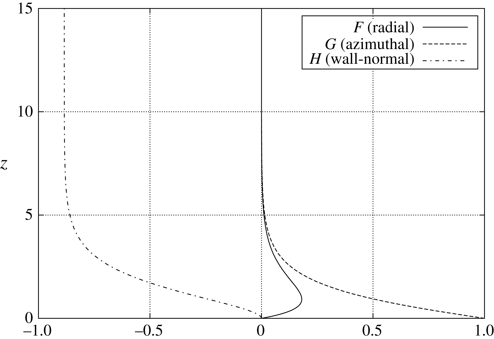
The von Kármán velocity profile.
2 Numerical formulation and numerical procedures
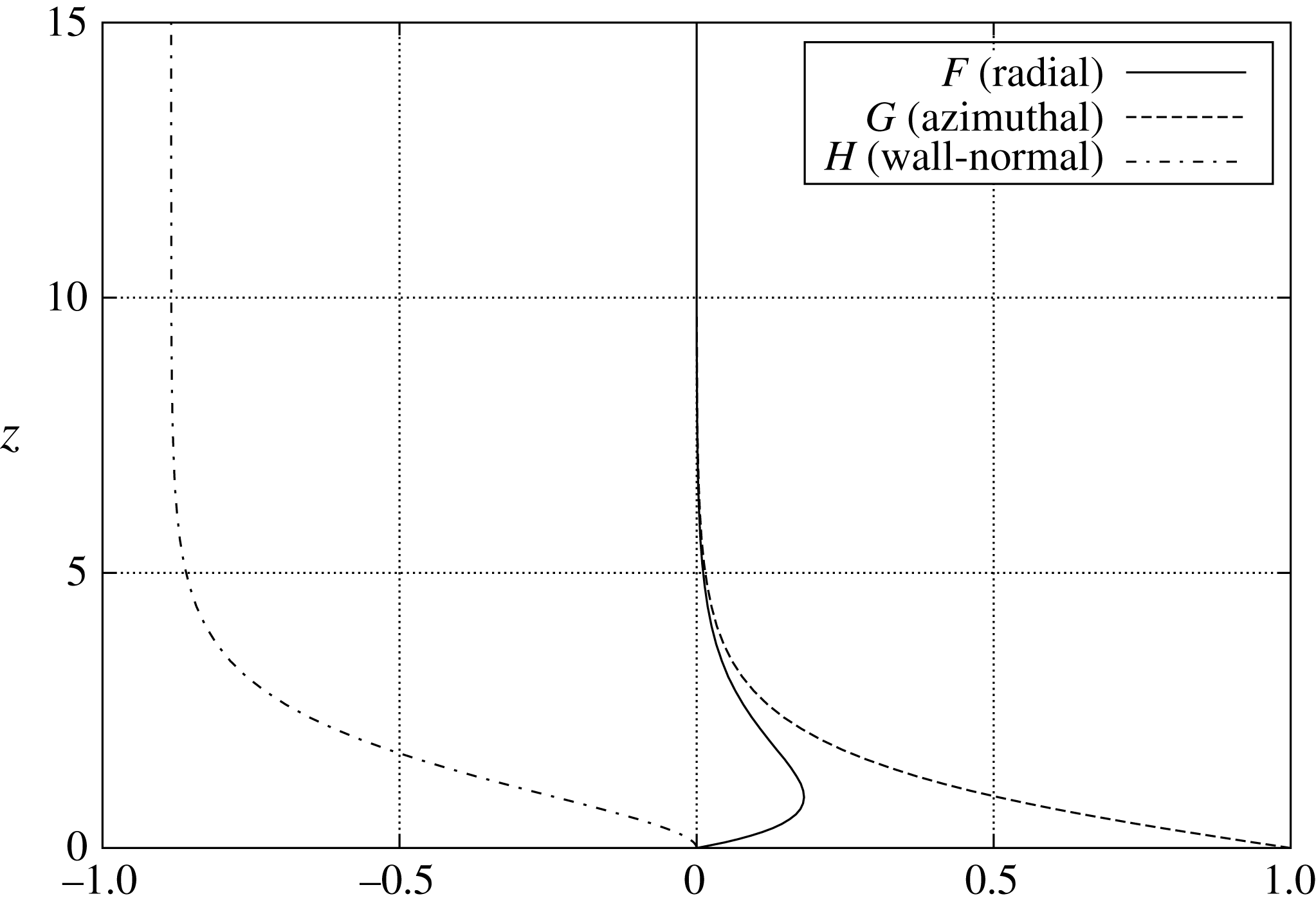
The stability of the 3D boundary layer that forms over a rotating disk in stationary fluid is studied by direct numerical solution of the full Navier–Stokes equations. For the steady infinite-disk flow of a viscous incompressible fluid, the thickness of the boundary layer is constant. Its velocity profile has an exact solution, named the von Kármán (Reference von Kármán1921) similarity solution, as shown in figure 1, which can be obtained by solving three ordinary differential equations,
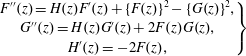 $$\begin{eqnarray}\left.\begin{array}{@{}c@{}}F^{\prime \prime }(z)=H(z)F^{\prime }(z)+\{F(z)\}^{2}-\{G(z)\}^{2},\\ G^{\prime \prime }(z)=H(z)G^{\prime }(z)+2F(z)G(z),\\ H^{\prime }(z)=-2F(z),\end{array}\right\}\end{eqnarray}$$
under the boundary conditions
 $$\begin{eqnarray}\left.\begin{array}{@{}c@{}}F(0)=0,\quad G(0)=1,\quad H(0)=0,\\ F(\infty )=0,\quad G(\infty )=0,\\ F^{\prime }(0)=0.510232618867,\quad G^{\prime }(0)=-0.615922014399,\end{array}\right\}\end{eqnarray}$$
using the fourth-order Runge–Kutta method. Here,
 $z$
is the normal distance from the disk. Variables
 $F(z)$
,
 $G(z)$
and
 $H(z)$
are defined as
 $$\begin{eqnarray}F(z)=\frac{U^{\ast }}{r^{\ast }\unicode[STIX]{x1D6FA}^{\ast }},\quad G(z)=\frac{V^{\ast }}{r^{\ast }\unicode[STIX]{x1D6FA}^{\ast }},\quad H(z)=\frac{W^{\ast }}{\sqrt{\unicode[STIX]{x1D708}^{\ast }\unicode[STIX]{x1D6FA}^{\ast }}},\end{eqnarray}$$
where
 $z$
is the normal distance from the disk and
 $^{\ast }$
denotes dimensional values. The variables
 $(U^{\ast },V^{\ast },W^{\ast })$
are the radial, azimuthal and wall-normal velocities, respectively, in the cylindrical polar coordinate,
 $r^{\ast }$
denotes the radial distance from the axis of rotation of the disk, and
 $\unicode[STIX]{x1D6FA}^{\ast }$
denotes the angular velocity. The boundary conditions for
 $F^{\prime }(0)$
and
 $G^{\prime }(0)$
in (2.2) are the same as in Miklavčič & Wang (Reference Miklavčič and Wang2004). It should be noted that a variable conversion is required for the wall-normal velocity component of the base flow,
 $H$
and
 $\tilde{W}$
, because different velocity scales are used for normalization.
In this study, this von Kármán velocity profile is used as a base flow, and only the perturbation components are computed. Therefore, the governing equations are the Navier–Stokes perturbation equations,
 $$\begin{eqnarray}\frac{\unicode[STIX]{x2202}\tilde{\boldsymbol{u}}}{\unicode[STIX]{x2202}\tilde{t}}+(\tilde{\boldsymbol{U}}+\tilde{\boldsymbol{u}})\boldsymbol{\cdot }\unicode[STIX]{x1D735}\tilde{\boldsymbol{u}}+\tilde{\boldsymbol{u}}\boldsymbol{\cdot }\unicode[STIX]{x1D735}\tilde{\boldsymbol{U}}=-\unicode[STIX]{x1D735}\tilde{p}+\frac{1}{\widetilde{Re}}\unicode[STIX]{x1D6FB}^{2}\tilde{\boldsymbol{u}}+\boldsymbol{f},\end{eqnarray}$$
and the continuity equation,
 $$\begin{eqnarray}\unicode[STIX]{x1D735}\boldsymbol{\cdot }\tilde{\boldsymbol{u}}=0,\end{eqnarray}$$
where
 $\tilde{\boldsymbol{u}}=(\tilde{u} ,\tilde{v},\tilde{w})$
and
 $\tilde{\boldsymbol{U}}=(\tilde{U} ,\tilde{V},\tilde{W})$
are the radial, azimuthal and wall-normal components of perturbation velocities and base-flow velocities, respectively, in cylindrical polar coordinates. Also,
 $\tilde{p}$
is pressure,
 $\tilde{t}$
is time, and a forcing term
 $\boldsymbol{f}$
is used in the sponge regions. All the variables in the governing equations are non-dimensionalized by the proper radius
 $r_{u}^{\ast }$
, the rotation velocity
 $r_{u}^{\ast }\unicode[STIX]{x1D6FA}^{\ast }$
, the time scale
 $r_{u}^{\ast }/(r_{u}^{\ast }\unicode[STIX]{x1D6FA}^{\ast })$
and the pressure
 $(r_{u}^{\ast }\unicode[STIX]{x1D6FA}^{\ast })^{2}\unicode[STIX]{x1D70C}$
, where
 $\unicode[STIX]{x1D708}^{\ast }$
is the kinematic viscosity and
 $\unicode[STIX]{x1D70C}^{\ast }$
is the density. The radius
 $r_{u}^{\ast }$
represents an arbitrary characteristic length. During this simulation, the value of
 $r_{u}^{\ast }$
is set to be unity for convenience. Thus, the Reynolds number for simulations is given by
 $$\begin{eqnarray}\widetilde{Re}=\frac{{r_{u}^{\ast }}^{2}\unicode[STIX]{x1D6FA}^{\ast }}{\unicode[STIX]{x1D708}^{\ast }}.\end{eqnarray}$$
From a physical point of view, it is convenient to use the thickness of the boundary layer
 $\sqrt{\unicode[STIX]{x1D708}^{\ast }/\unicode[STIX]{x1D6FA}^{\ast }}$
instead of
 $r_{u}^{\ast }$
as a length scale, and also to use the local rotation velocity
 $r^{\ast }\unicode[STIX]{x1D6FA}^{\ast }$
instead of
 $r_{u}^{\ast }\unicode[STIX]{x1D6FA}^{\ast }$
as a velocity scale. Therefore, the Reynolds number is defined again as
 $$\begin{eqnarray}Re=\frac{\sqrt{\unicode[STIX]{x1D708}^{\ast }/\unicode[STIX]{x1D6FA}^{\ast }}\,r^{\ast }\unicode[STIX]{x1D6FA}^{\ast }}{\unicode[STIX]{x1D708}^{\ast }}=r^{\ast }\sqrt{\frac{\unicode[STIX]{x1D6FA}^{\ast }}{\unicode[STIX]{x1D708}^{\ast }}}=r,\end{eqnarray}$$
which means that this Reynolds number
 $Re$
is equivalent to the non-dimensional radial position
 $r$
on the disk. Similarly, the velocity components
 $\tilde{\boldsymbol{u}}$
and
 $\tilde{\boldsymbol{U}}$
are converted to
 $\boldsymbol{u}=(u,v,w)$
and
 $\boldsymbol{U}=(U,V,W)$
. The rotation number of the disk is defined as
 $T$
=
 $t^{\ast }\unicode[STIX]{x1D6FA}^{\ast }/2\unicode[STIX]{x03C0}$
.
The governing equations (2.4) and (2.5) are solved by a finite difference method (the MAC method). The second-order Crank–Nicolson semi-implicit scheme is used for time advancement. For discretization of spatial derivative terms, the third-order upwind difference scheme (Kawamura, Takami & Kuwahara Reference Kawamura, Takami and Kuwahara1986) is applied only to the convection terms, and the fourth-order central difference scheme is applied to the other terms. A 27-colour SOR method is used to solve the Poisson equation. All the simulations are performed on a multi-GPU platform, which consists of four GPU cards (Nvidia GTX-TITAN) for faster and parallelized computation.
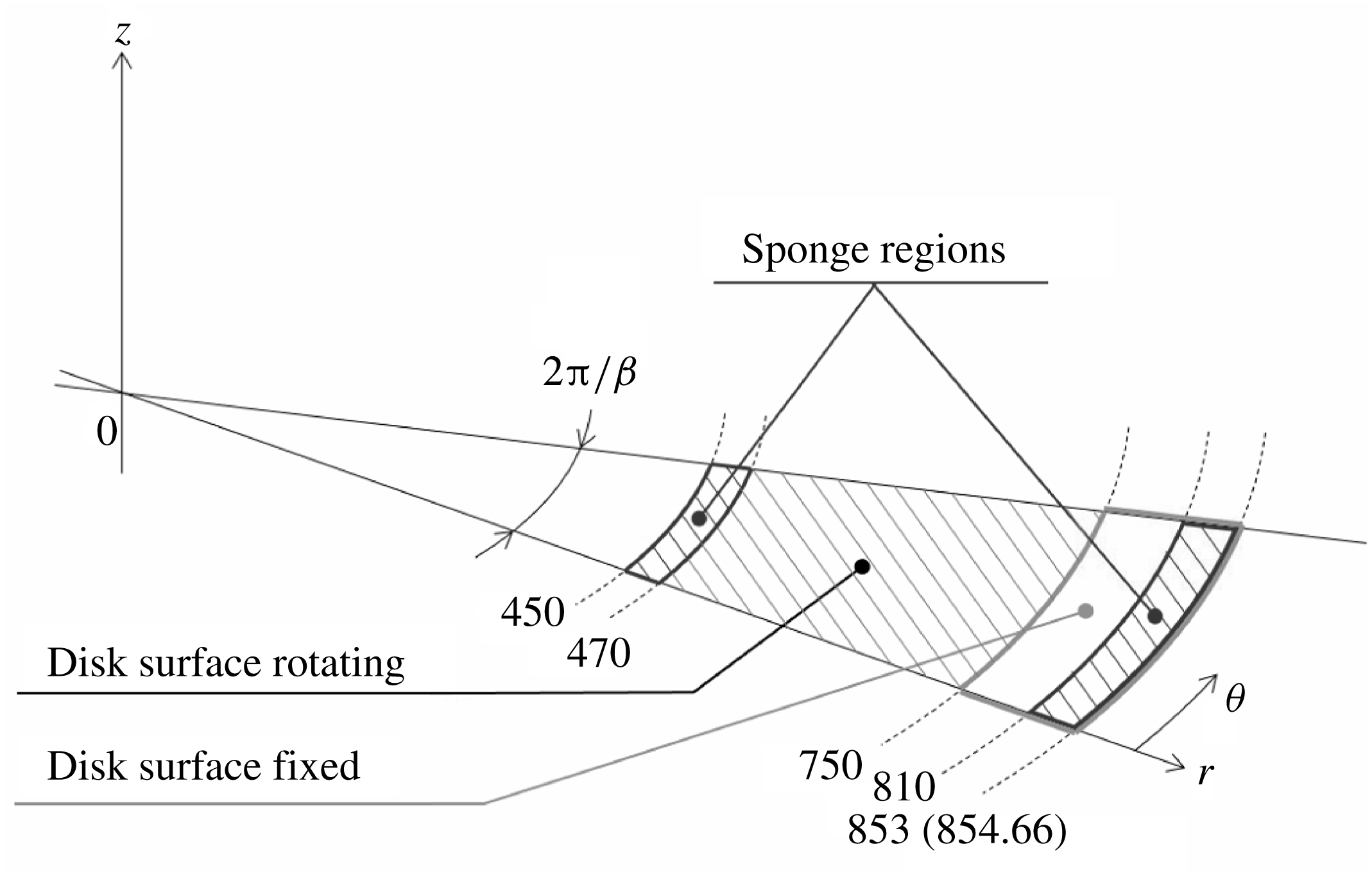
Computational domain.
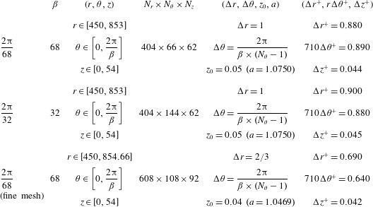
Computational conditions for
 $2\unicode[STIX]{x03C0}/68$
,
 $2\unicode[STIX]{x03C0}/32$
and
 $2\unicode[STIX]{x03C0}/68$
(fine mesh). The parameters are the azimuthal wavenumber
 $\unicode[STIX]{x1D6FD}$
, the radial, azimuthal and wall-normal grid numbers
 $N_{r}$
,
 $N_{\unicode[STIX]{x1D703}}$
and
 $N_{z}$
, respectively, the grid resolutions
 $\unicode[STIX]{x0394}r$
,
 $\unicode[STIX]{x0394}\unicode[STIX]{x1D703}$
,
 $z_{0}$
and
 $a$
, and the wall units
 $\unicode[STIX]{x0394}r^{+}$
,
 $r\unicode[STIX]{x0394}\unicode[STIX]{x1D703}^{+}$
,
 $\unicode[STIX]{x0394}z^{+}$
at
 $Re=710$
.
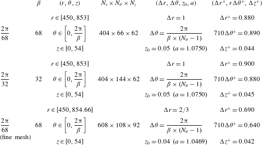
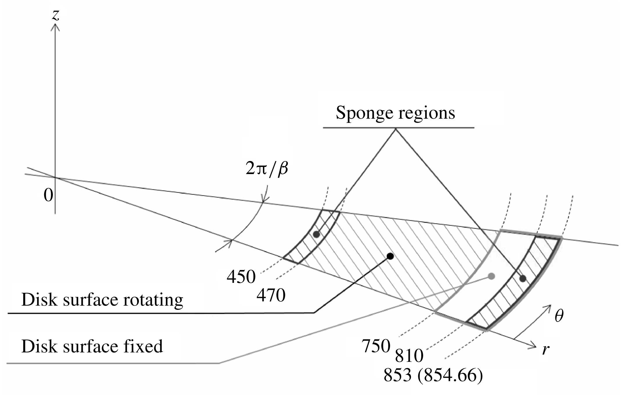
The computational domain is illustrated in figure 2, and the computational parameters are listed in table 1. Inside radius 750, the disk surface is rotating, while the surface outside is not moving. To reduce the computational cost, the domain is limited to a fan-shaped region instead of a full circular disk. Periodic boundary conditions are used in the azimuthal direction. The domain covers the region of
 $450\leqslant r\leqslant 853$
(or 854.66 for the fine mesh case in table 1),
 $0\leqslant \unicode[STIX]{x1D703}\leqslant 2\unicode[STIX]{x03C0}/\unicode[STIX]{x1D6FD}$
and
 $0\leqslant z\leqslant 54$
. For azimuthal wavenumber
 $\unicode[STIX]{x1D6FD}$
, 68 or 32 are selected. The azimuthal wavenumber
 $\unicode[STIX]{x1D6FD}=68$
is the critical azimuthal wavenumber for the onset of absolute instability, according to the theoretical prediction of Lingwood (Reference Lingwood1995). Azimuthal wavenumber
 $\unicode[STIX]{x1D6FD}=32$
is the typical number of stationary vortices observed at higher Reynolds number, and
 $\unicode[STIX]{x1D6FD}=24{-}26$
is more typical at lower Reynolds number. Numerical simulations are carried out under the following three grid conditions. The
 $2\unicode[STIX]{x03C0}/68$
computation is a base condition for
 $\unicode[STIX]{x1D6FD}=68$
. In the
 $2\unicode[STIX]{x03C0}/32$
region computation, the computational domain is much larger in the azimuthal direction, which can check the effect of the periodic boundary condition in this direction. We also checked grid dependence by comparing the ordinary mesh
 $2\unicode[STIX]{x03C0}/68$
computation with the fine mesh
 $2\unicode[STIX]{x03C0}/68$
computation, which has 1.5 times greater resolution in each direction. In all cases, the grids are concentrated near the disk by a geometric series of a common ratio of
 $a$
and the first term of
 $z_{n}$
, which is
 $z_{0}$
. Thus, the wall-normal location is given by
 $$\begin{eqnarray}z_{n}=z_{0}\frac{a^{n_{z}}-1}{a-1},\end{eqnarray}$$
where
 $n_{z}$
is the
 $n$
th grid number in the wall-normal direction. The values of
 $a$
and the first term
 $z_{0}$
are given in table 1.
As an artificial disturbance, wall-normal short-duration suction and blowing was performed from an annular slit of width 4 in the disk surface. The Reynolds number of the suction and blowing location,
 $Re=598{-}602$
, is higher than the critical Reynolds number for the global instability,
 $Re=583$
for
 $\unicode[STIX]{x1D6FD}=68$
, which is approximately equal to the critical Reynolds number for the global instability,
 $Re=599$
for
 $\unicode[STIX]{x1D6FD}=64$
(Appelquist et al.
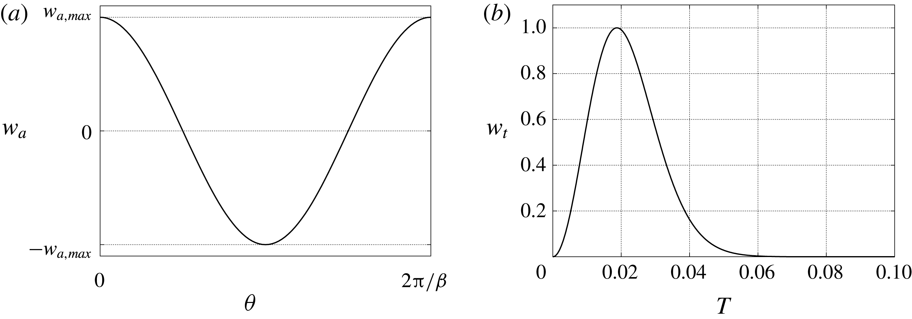
Reference Appelquist, Schlatter, Alfredsson and Lingwood2018). Relatively strong suction and blowing was used to quickly establish a wavy structure in the flow field. The velocity profiles of the suction and blowing consist of two parts: the spatial amplitude
 $w_{a}$
depending on the azimuthal direction, and the temporal amplitude
 $w_{t}$
,
 $$\begin{eqnarray}w_{excite}(\unicode[STIX]{x1D703},t)=w_{a}(\unicode[STIX]{x1D703},t)w_{t}(t).\end{eqnarray}$$
These two terms are given by
 $$\begin{eqnarray}\displaystyle & w_{a}(\unicode[STIX]{x1D703},t)=w_{a,max}\cos (\unicode[STIX]{x1D6FD}(\unicode[STIX]{x1D703}-t)), & \displaystyle\end{eqnarray}$$
 $$\begin{eqnarray}\displaystyle & w_{t}(t)=4(1-\text{e}^{-50t^{2}})\text{e}^{-50t^{2}}, & \displaystyle\end{eqnarray}$$
where
 $w_{a,max}=0.1V$
,
 $0<\unicode[STIX]{x1D703}<2\unicode[STIX]{x03C0}/\unicode[STIX]{x1D6FD}$
and
 $0<t<0.06\times 2\unicode[STIX]{x03C0}$
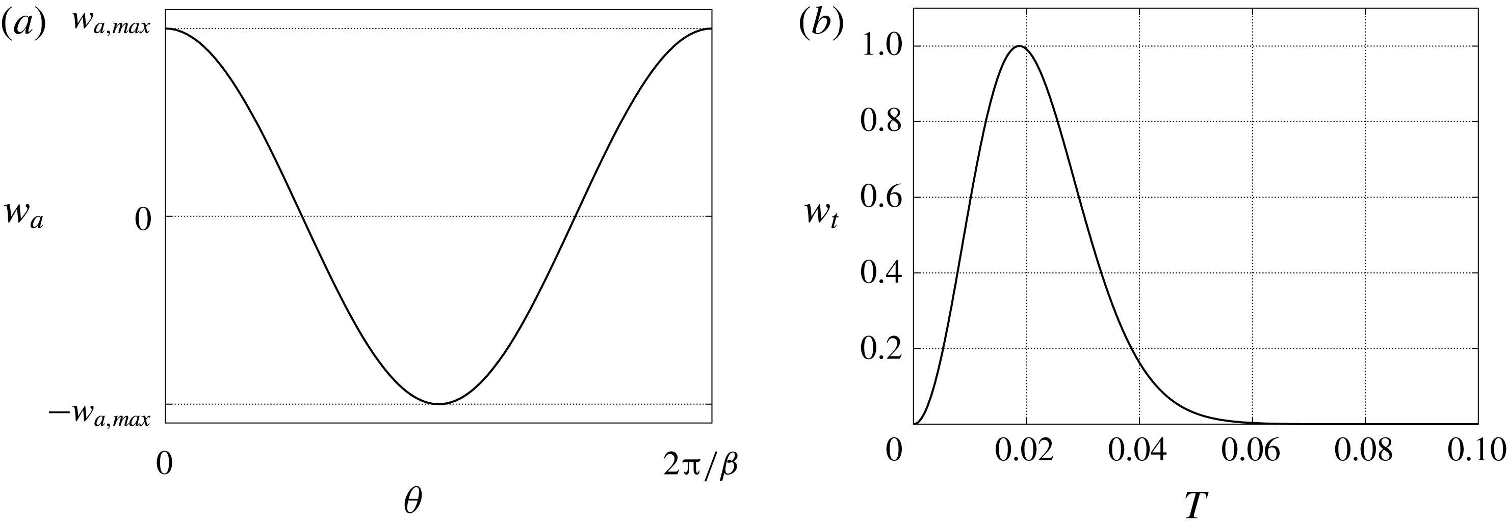
. Figure 3 shows the initial spatial amplitude
 $w_{a}(\unicode[STIX]{x1D703},0)$
and the temporal amplitude
 $w_{t}(t)$
. In figure 3,
 $T$
is the number of rotations, which is
 $T=t/2\unicode[STIX]{x03C0}$
. The azimuthal wavenumber of the disturbance is set to be equal to the azimuthal number of the computational domain,
 $\unicode[STIX]{x1D6FD}$
. The forcing disturbance, which is the short-duration suction and blowing, is always stationary relative to the rotating-disk surface, because it has the same angular velocity as the rotating disk.
(a) The initial spatial amplitude
 $w_{a}(\unicode[STIX]{x1D703},0)$
of the artificial disturbance. (b) The temporal amplitude
 $w_{t}(t)$
of the artificial disturbance.
2.1 Boundary conditions and initial condition
The boundary conditions for the perturbation components are determined by referring to the conditions of Appelquist et al. (Reference Appelquist, Schlatter, Alfredsson and Lingwood2015a
). During the present simulations, the von Kármán (Reference von Kármán1921) similarity solution, which is obtained by the preliminary computation, is used as the base flow of the 3D rotating-disk boundary layer. The disk surface is rotating in the region from the inlet (
 $Re=450$
) to
 $Re=750$
, while it stands still in the region of
 $Re>750$
. This configuration is the same as that of the experimental study by Imayama, Alfredsson & Lingwood (Reference Imayama, Alfredsson and Lingwood2014). Thus, we use two different non-slip boundary conditions for fluctuating components in accordance with the rotational and irrotational parts of the disk. The former boundary conditions are given by
 $$\begin{eqnarray}\tilde{u} =\tilde{v}=\tilde{w}=0,\end{eqnarray}$$
and the latter boundary conditions are
 $$\begin{eqnarray}\tilde{u} =0,\quad \tilde{v}=-\frac{r^{\ast }\unicode[STIX]{x1D6FA}^{\ast }}{r_{u}^{\ast }\unicode[STIX]{x1D6FA}^{\ast }},\quad \tilde{w}=0.\end{eqnarray}$$
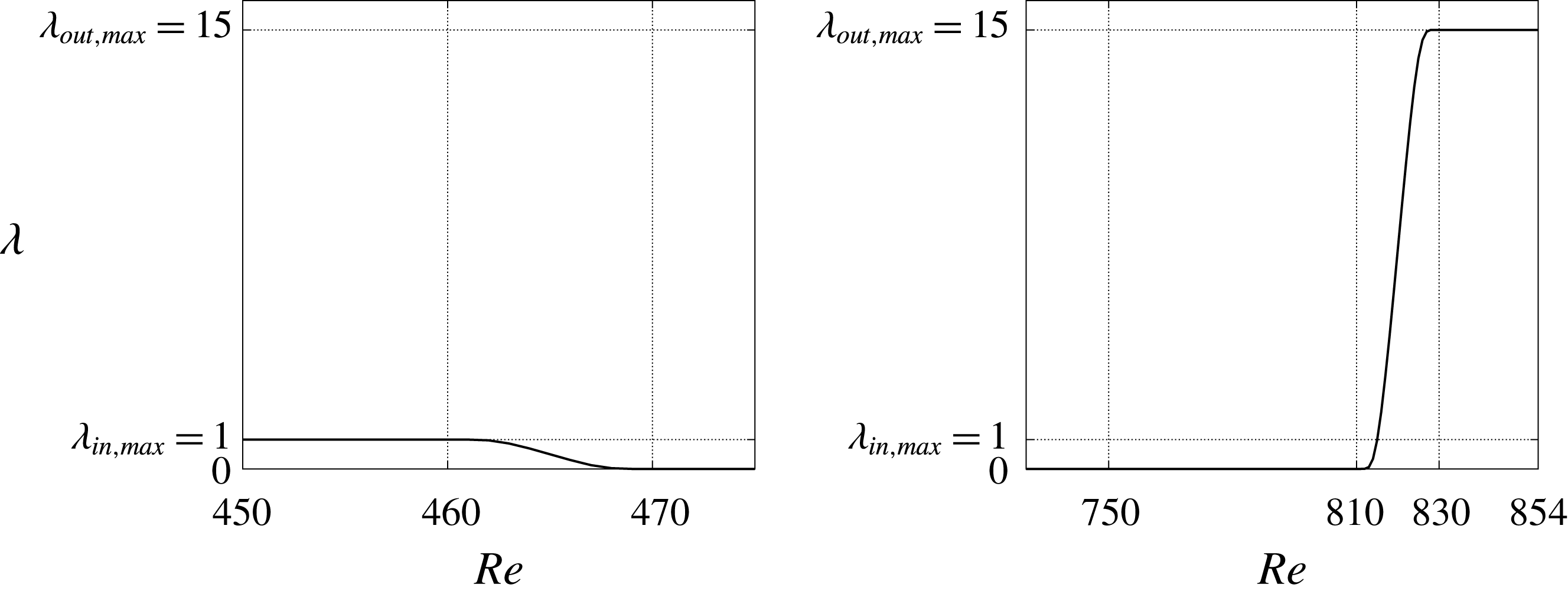
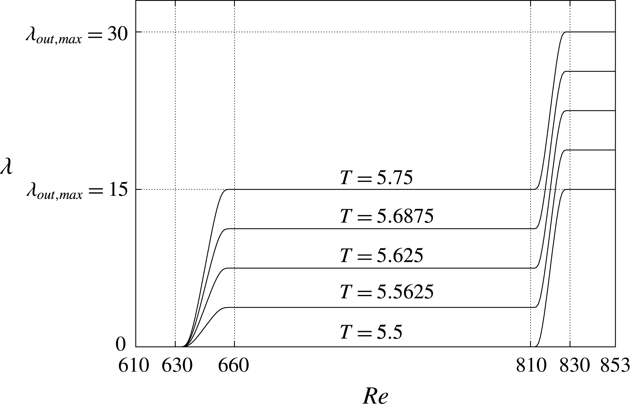
First, a conventional Neumann condition for the outflow boundary was tested, which ended up with contamination of the inflow due to undesirable reflections at the outflow boundary as the turbulent fluid flowed out. In order to prevent such contamination by non-physical reflections, sponge regions were introduced, where the velocity fluctuations were forced to be damped to a sufficiently weak level at which the mean flow could be assumed to be equal to the base flow. The sponge regions were placed at both the inflow and outflow boundaries, as shown in figure 2. The sponge function is defined as
 $$\begin{eqnarray}\boldsymbol{f}=-\unicode[STIX]{x1D706}(Re)\tilde{\boldsymbol{u}},\end{eqnarray}$$
where the function
 $\unicode[STIX]{x1D706}(Re)$
is given by
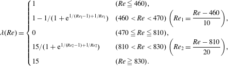 $$\begin{eqnarray}\unicode[STIX]{x1D706}(Re)=\left\{\begin{array}{@{}ll@{}}1 & (Re\leqq 460),\\ 1-1/(1+\text{e}^{1/(Re_{1}-1)+1/Re_{1}}) & (460<Re<470)\left(Re_{1}={\displaystyle \frac{Re-460}{10}}\right)\!,\\ 0 & (470\leqq Re\leqq 810),\\ 15/(1+\text{e}^{1/(Re_{2}-1)+1/Re_{2}}) & (810<Re<830)\left(Re_{2}={\displaystyle \frac{Re-810}{20}}\right)\!,\\ 15 & (Re\geqq 830).\end{array}\right.\end{eqnarray}$$
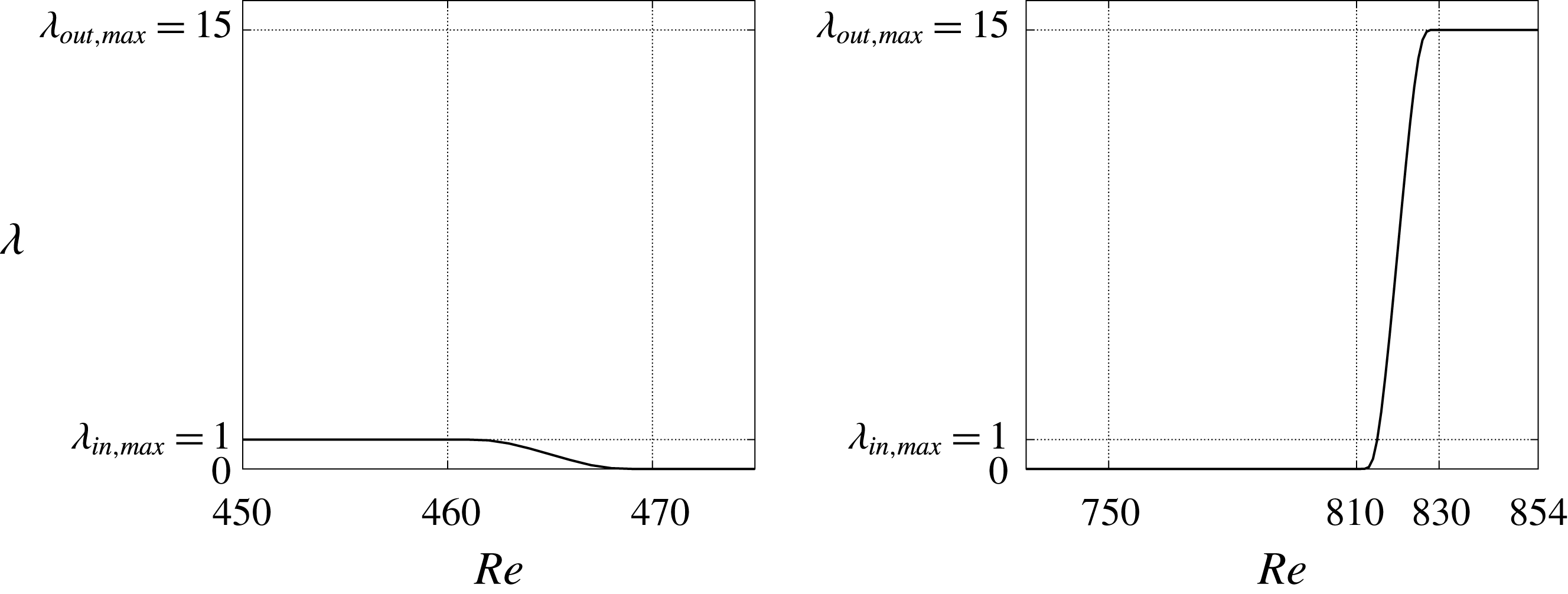
Figure 4 shows the profile of sponge function
 $\unicode[STIX]{x1D706}(Re)$
, where
 $\unicode[STIX]{x1D706}_{in,max}$
is 1, and
 $\unicode[STIX]{x1D706}_{out,max}$
is 15 for all computations. The inlet sponge region is from the inlet through
 $Re=470$
. The outlet sponge region is
 $Re>810$
, right after the stationary disk given as the non-slip condition region,
 $Re=750{-}810$
. The perturbation velocities are set to zero at the upstream and downstream boundaries in the radial direction. The perturbation components
 $\tilde{u} ,~\tilde{v}$
are zero and
 $\text{d}w/\text{d}z=p$
on the upper boundary surface, which is the same as in Appelquist et al. (Reference Appelquist, Schlatter, Alfredsson and Lingwood2015a
). Because of the non-slip boundary condition, it takes time to reach a steady state. Therefore, the flow field after 1.5 rotations is used as the initial flow condition.
The values of sponge function in the entire radial direction;
 $\unicode[STIX]{x1D706}_{in,max}$
and
 $\unicode[STIX]{x1D706}_{out,max}$
are the maximum values at the inflow and outflow regions, respectively.
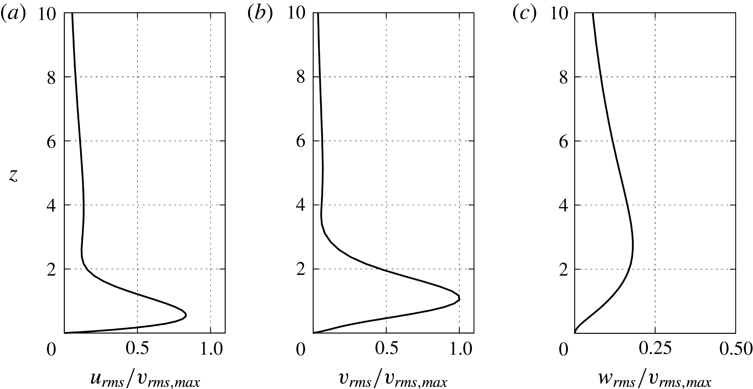
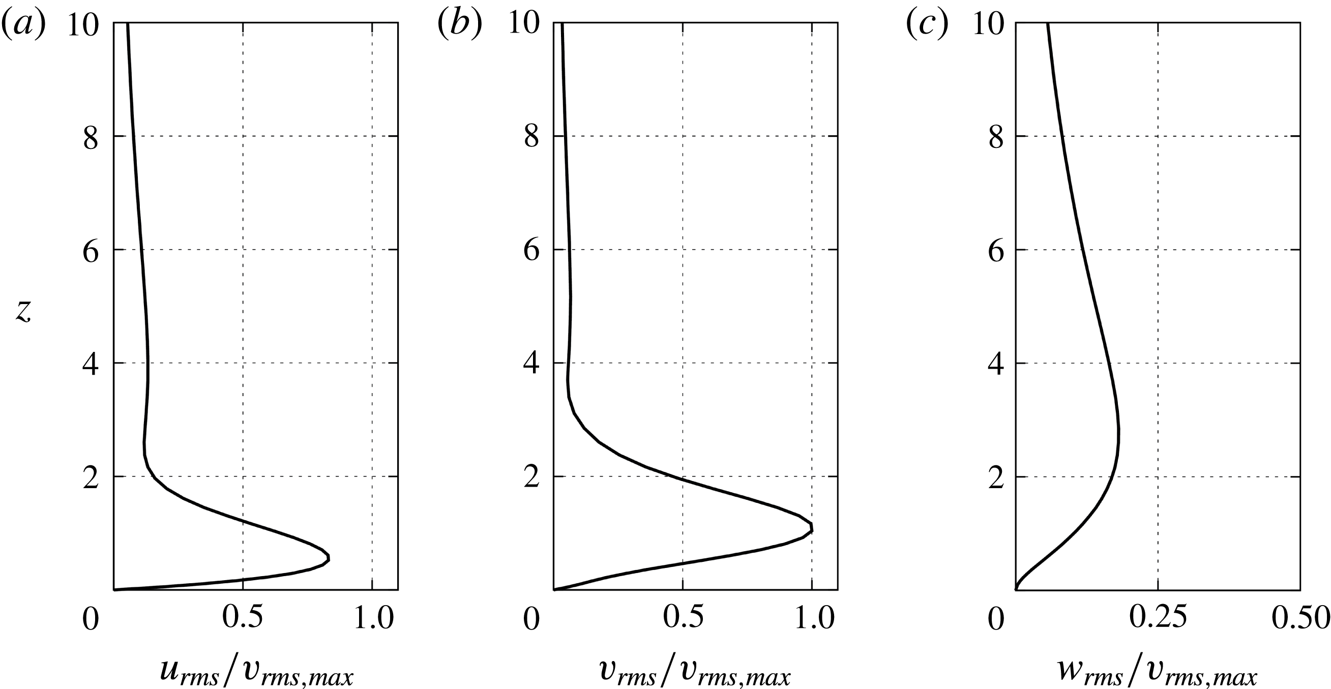
The r.m.s. values of velocity fluctuation components in each direction (
 $r,\unicode[STIX]{x1D703},z$
) at
 $Re=570$
for
 $2\unicode[STIX]{x03C0}/68$
computation. All the profiles are normalized by the maximum value of the azimuthal profile.
3 Results and discussion
3.1 Computation in
 $2\unicode[STIX]{x03C0}/68$
domain and code verification

We compared our results with other DNS data in order to verify the validity of our simulation code.
Figure 5 shows the root-mean-square (r.m.s.) profiles of velocity fluctuation components in each direction after the growth rate of the flow field reached a steady state. Appelquist et al. (Reference Appelquist, Schlatter, Alfredsson and Lingwood2016b
) used a short volume force to disturb the flow, whereas we used a local suction and blowing in our computation. Data of radial locations,
 $Re=570$
, are presented. The locations are the same as in figure 10 of Appelquist et al. (Reference Appelquist, Schlatter, Alfredsson and Lingwood2016b
). The r.m.s. values of each velocity fluctuation component are given by
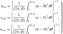 $$\begin{eqnarray}\left.\begin{array}{@{}c@{}}\displaystyle u_{rms}=\left[\frac{1}{(2\unicode[STIX]{x03C0}/\unicode[STIX]{x1D6FD})}\int _{0}^{2\unicode[STIX]{x03C0}/\unicode[STIX]{x1D6FD}}(u-\overline{u})^{2}\,\text{d}\unicode[STIX]{x1D703}\right]^{1/2}\!,\\ \displaystyle v_{rms}=\left[\frac{1}{(2\unicode[STIX]{x03C0}/\unicode[STIX]{x1D6FD})}\int _{0}^{2\unicode[STIX]{x03C0}/\unicode[STIX]{x1D6FD}}(v-\overline{v})^{2}\,\text{d}\unicode[STIX]{x1D703}\right]^{1/2}\!,\\ \displaystyle w_{rms}=\left[\frac{1}{(2\unicode[STIX]{x03C0}/\unicode[STIX]{x1D6FD})}\int _{0}^{2\unicode[STIX]{x03C0}/\unicode[STIX]{x1D6FD}}(w-\overline{w})^{2}\,\text{d}\unicode[STIX]{x1D703}\right]^{1/2}\!,\end{array}\right\}\end{eqnarray}$$
where the bar denotes the mean value. At each streamwise location, the data are normalized by the maximum value of
 $v_{rms,max}$
at that location. The profiles of the present simulation agree well with those of Appelquist et al. (Reference Appelquist, Schlatter, Alfredsson and Lingwood2016b
). From the results, we concluded that there were no problems with our code in simulating the behaviour of disturbance introduced from the upstream surface of the rotating disk.
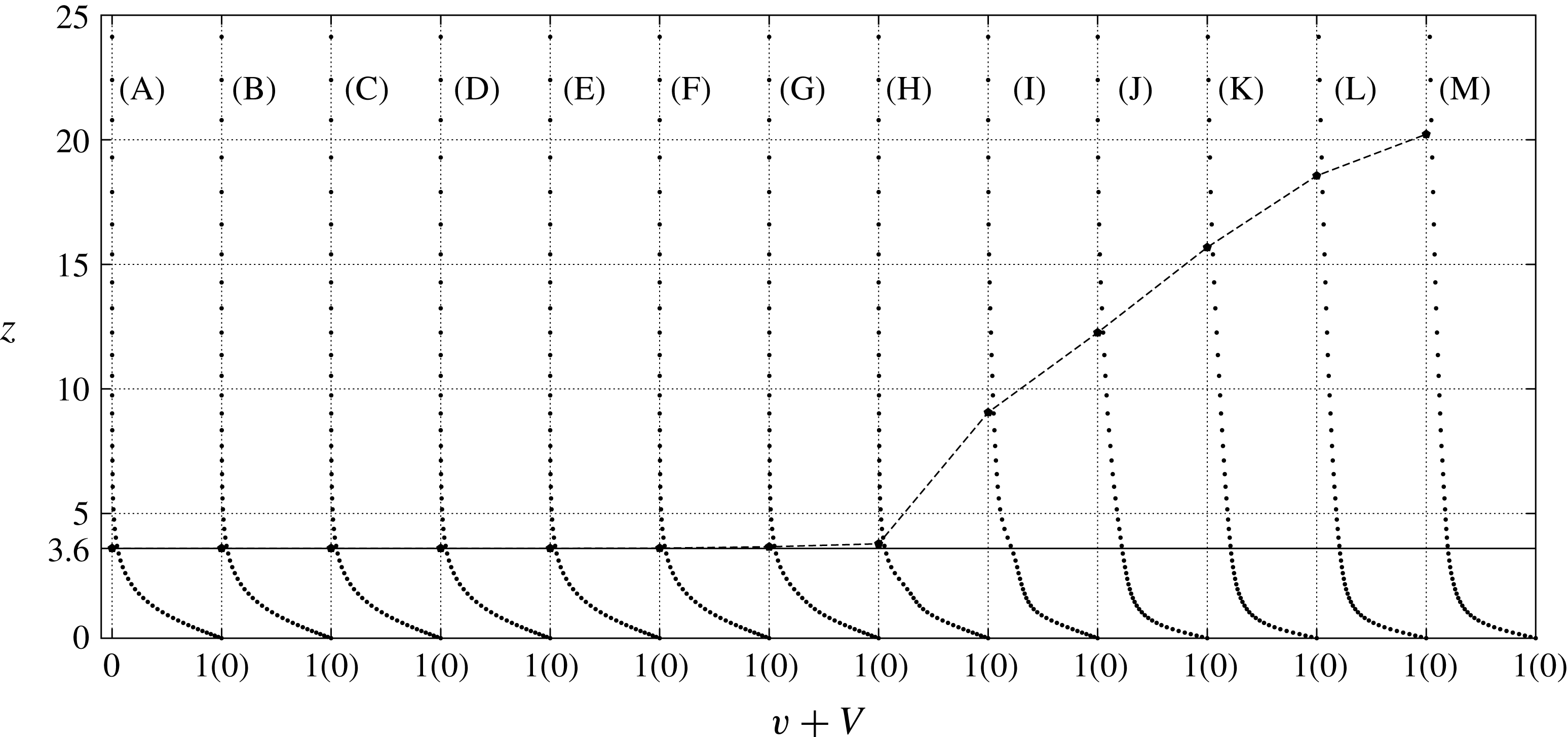
Profiles of the mean azimuthal velocity for the
 $2\unicode[STIX]{x03C0}/68$
region computation at different radial locations:
 $Re=490$
(A), 510 (B), 530 (C), 550 (D), 570 (E), 590 (F), 610 (G), 630 (H), 650 (I), 670 (J), 690 (K), 710 (L) and 730 (M). The solid straight line at
 $z=3.6$
indicates the theoretical boundary layer thickness for the laminar profile, which is defined as the height where
 $V=0.05$
. The velocity data are spatially averaged in the azimuthal direction and temporally averaged for
 $T=3.5{-}5.5$
, which is after the flow field reaches the steady state. The location of the boundary layer outer edge is also shown by a broken line.
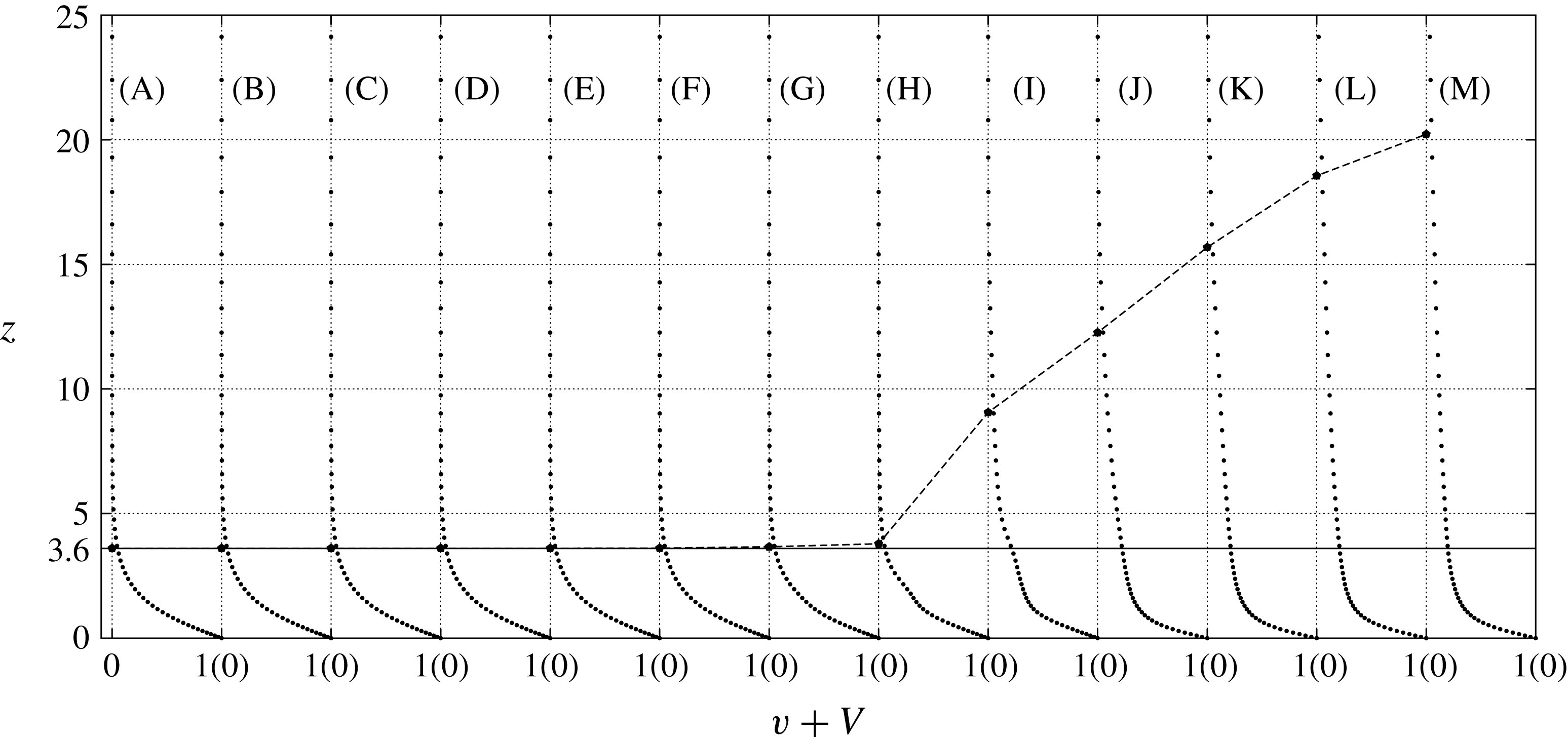
Figure 6 shows the profiles of the total mean velocity in the azimuthal direction at different radial locations
 $Re=490{-}730$
. The location of the boundary layer outer edge, which is defined as
 $V=0.05$
, is also shown in figure 6. The azimuthal velocity component for the
 $2\unicode[STIX]{x03C0}/68$
region computation is spatially and temporally averaged at each location through the rotation number
 $T=3.5{-}5.5$
, which is after the flow field has reached a steady state. The velocity profiles are self-similar, and the boundary layer thickness is kept constant at
 $z=3.6$
throughout the laminar region, which is upstream of
 $Re<630$
. The results agree with the von Kármán similarity solution. When the Reynolds number exceeds 630, the boundary layer thickness increases considerably, and the velocity gradient near the wall becomes larger. The boundary layer thickness reaches 20 at
 $Re=730$
. The velocity profiles at these higher Reynolds numbers become close to those of fully turbulent boundary layers. The results agree with the experimental study by Imayama et al. (Reference Imayama, Alfredsson and Lingwood2014), although the deviation from the laminar profile starts at the smaller Reynolds number of 550 in their case. The reason for the discrepancy is probably that, in the experiments, minute roughness is unavoidable on a real disk surface, which would continuously excite the stationary mode. Appelquist et al. (Reference Appelquist, Schlatter, Alfredsson and Lingwood2016a
) studied the linear effect of distributed roughness on the stationary convective modes and showed that good agreement is present among the local linear stability analysis, DNS in a linear framework and experiment.
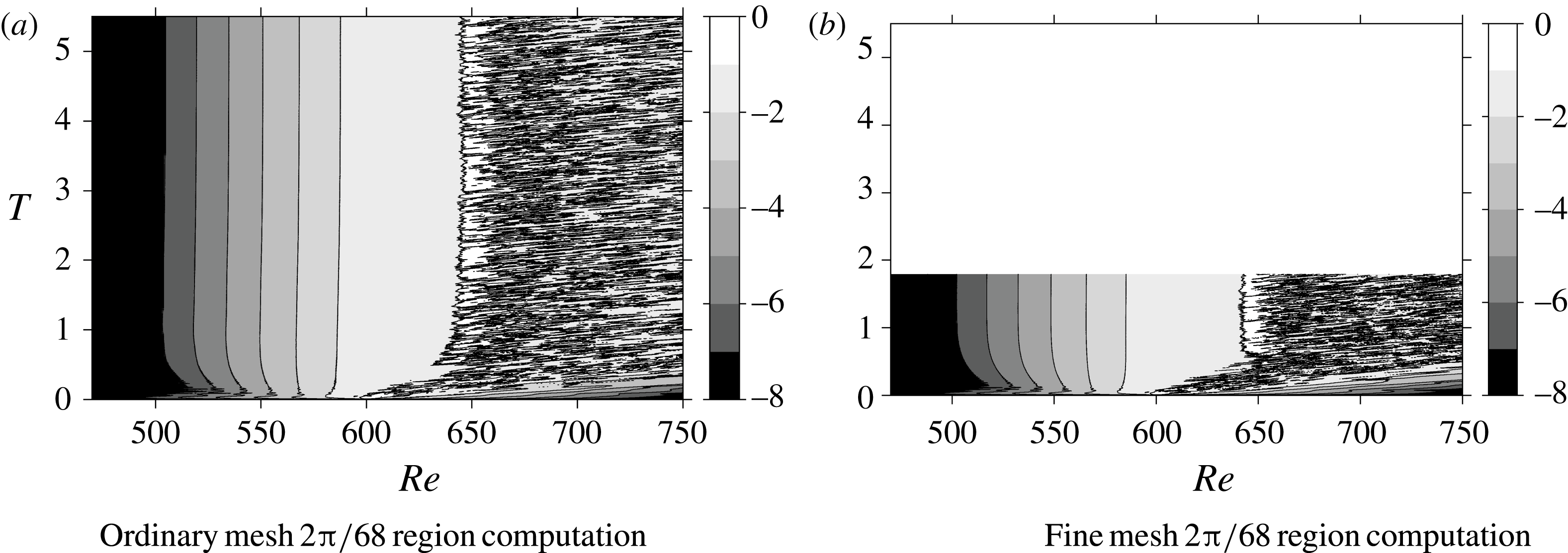
Figure 7(a) shows the spatial and temporal developments of
 $\log (v_{rms})$
measured at
 $z=1.3$
. The initial local disturbance is added at
 $Re\approx 600$
. The strong, highly unsteady velocity fluctuation, represented by the numerous black lines in the white area, is convected downstream up to approximately
 $T=0.7{-}0.8$
. After that, all the borders between the different levels of velocity fluctuations become parallel, which indicates that the distribution becomes steady. Downstream of
 $Re>640$
, a fully turbulent region is formed. Another simulation with a finer grid resolution was performed to investigate the influence of grid resolution on the numerical results; the results are shown in figure 7(b) as the case for
 $2\unicode[STIX]{x03C0}/68$
(fine mesh). In this case, the computation was terminated at
 $T=1.8$
, because the flow field became steady and the profile stopped changing with time. Little difference in the computational results could be found between the two cases, which confirms that the grid used in the ordinary mesh case was sufficiently fine. These results also agree with the DNS by Appelquist et al. (Reference Appelquist, Schlatter, Alfredsson and Lingwood2015b
), which had the outflow boundary at
 $Re=700$
. From the comparison, we determined that our simulation code has sufficient accuracy to analyse the flow field on the rotating disk.
Spatio-temporal development of
 $\log (v_{rms})$
at
 $z=1.3$
for different grid resolutions: (a) ordinary mesh and (b) fine mesh. The colour bar indicates the value of
 $\log (v_{rms})$
.
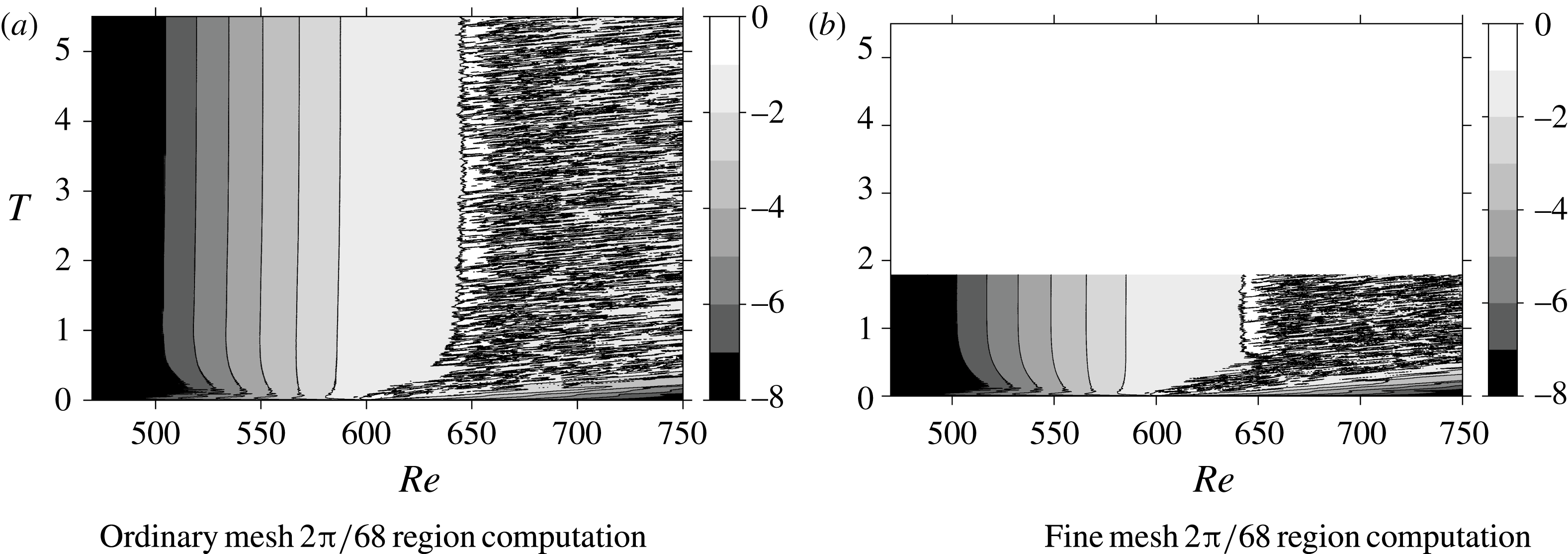
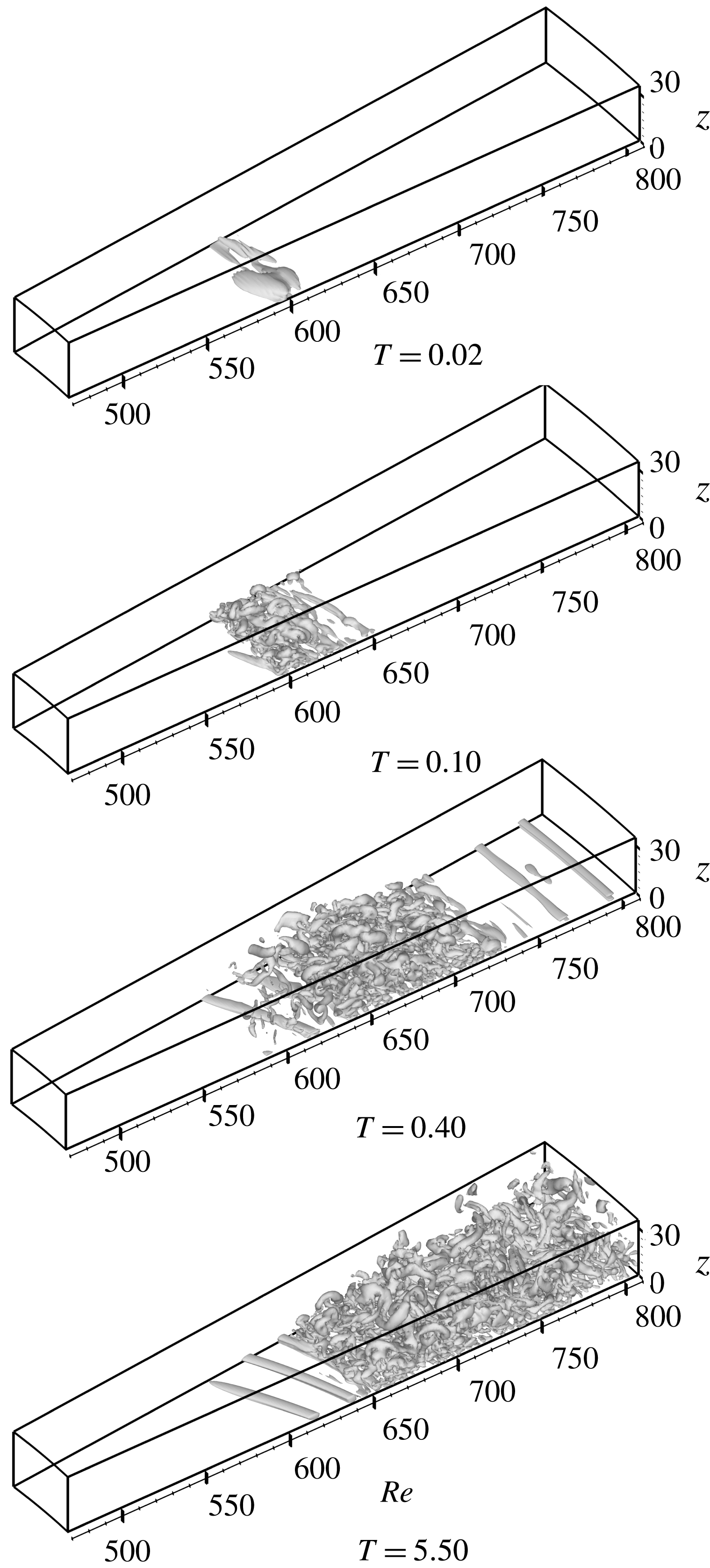
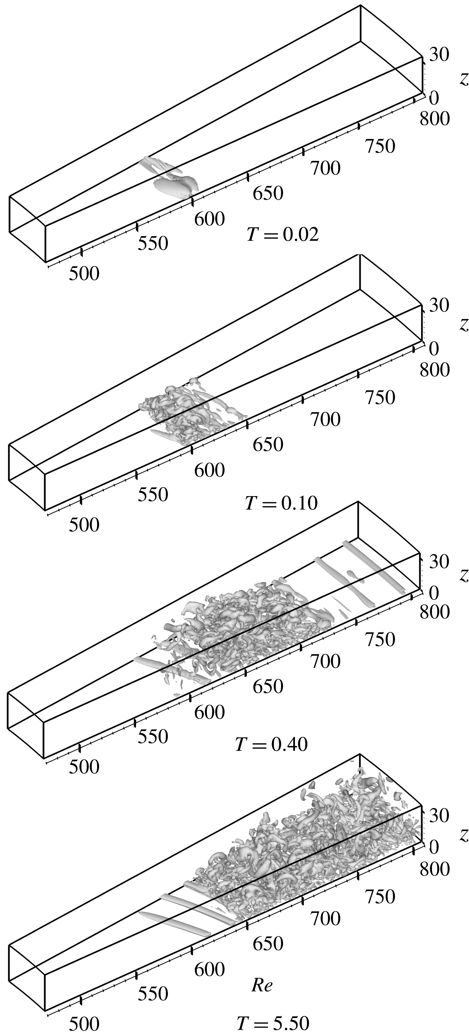
Figure 8 shows the isosurface of the second invariant of velocity gradient tensor
 $\unicode[STIX]{x1D64C}$
at
 $\unicode[STIX]{x1D64C}=50$
for the case of
 $2\unicode[STIX]{x03C0}/68$
. In figure 8, vortical structures at
 $T=0.02$
, 0.10, 0.40 and 5.50 are shown, where
 $T=0.02$
is the moment at which the disturbance amplitude reaches its maximum, and
 $T=5.5$
is after the flow field reaches the steady state. A disturbance is added to the boundary layer at
 $Re=598{-}602$
, which is in the region where global instability is unstable. The disturbance grows while flowing down in the radial direction, and by
 $T=0.1$
, a complicated vortical structure, which represents turbulence, is formed. When the flow field settles down, as by
 $T=5.5$
, a turbulent flow can be found in a large area downstream around
 $Re=640{-}650$
. Also at
 $T=5.5$
, spiral vortices can be clearly observed in the region
 $Re=590{-}640$
, upstream of the turbulent region. At
 $T=0.4$
, the axisymmetric vortices can be observed on the stationary disk surface at
 $Re=750{-}800$
. They are transient structures, which later will be covered by the upstream turbulent region.
Isosurface of
 $\unicode[STIX]{x1D64C}=50$
at
 $T=0.02$
, 0.1, 0.4 and 5.5 for the ordinary mesh
 $2\unicode[STIX]{x03C0}/68$
region computation case.
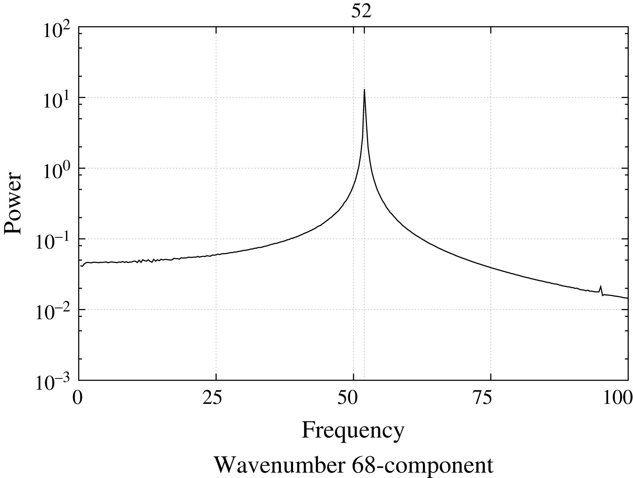
The temporal power spectrum of the azimuthal velocities for wavenumber 68-component at
 $z=1.3$
and
 $Re=610$
is shown in figure 9. The spectrum is calculated using 750 data points of
 $T=2.5{-}5.5$
; thus the resolution of the temporal wavenumber becomes
 $1/3$
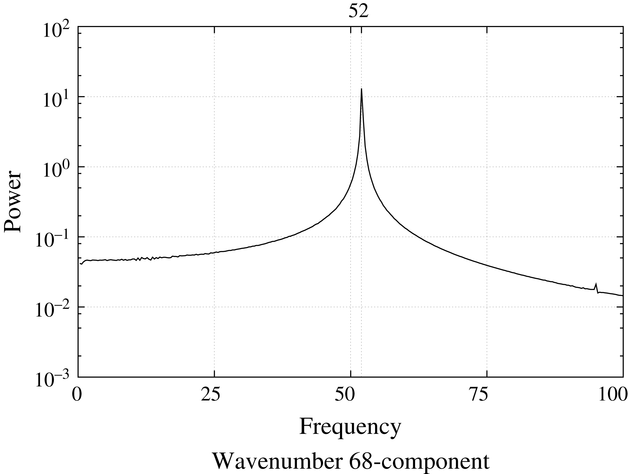
. The data are the same as what a hot wire would measure in an experiment. The horizontal axis in figure 9 indicates the temporal wavenumber per rotation of the disk. Henceforward, this temporal wavenumber is called the frequency. The frequency of the wavenumber 68-component measured in the laboratory frame is 52. The frequency in the rotating frame can be calculated by subtracting the wavenumber component from the frequency in the laboratory frame, i.e.
 $52-68=-16$
. This result shows that the 68 spiral vortices are not stationary with respect to the rotating disk, but are travelling in the azimuthal direction. In addition, this value of
 $-16$
is very close to the frequencies of wavenumber 68-component in the linear simulation of Appelquist et al. (Reference Appelquist, Schlatter, Alfredsson and Lingwood2015a
), the nonlinear simulation of Appelquist et al. (Reference Appelquist, Schlatter, Alfredsson and Lingwood2016b
) and the theoretical prediction of Lingwood (Reference Lingwood1995), which are
 $-15.86$
to
 $-15.96$
,
 $-15.64$
and
 $-15.56$
, respectively.
Frequency spectrum of
 $v$
at
 $z=1.3$
and
 $Re=610$
for the wavenumber 68-component, using the data of
 $2.5{-}5.5$
rotations.
3.2 Computation in the
$2\unicode[STIX]{x03C0}/32$
domain

The growth of impulsive disturbance excited at
 $Re\approx 600$
is also studied using a computational domain larger in the azimuthal direction,
 $2\unicode[STIX]{x03C0}/32$
, because this larger domain can handle also the circumferential wavenumber 32, corresponding to 32 spiral vortices for the whole disk. The number 32 is the most likely number of spiral vortices found in the experiments (Kobayashi et al.
Reference Kobayashi, Kohama and Takamadate1980; Malik et al.
Reference Malik, Wilkinson and Orszag1981; Jarre, Gal & Chauve Reference Jarre, Gal and Chauve1995; Imayama et al.
Reference Imayama, Alfredsson and Lingwood2013). The flow field is disturbed for a very short period at
 $Re\approx 600$
, as a fluctuation of the
 $w$
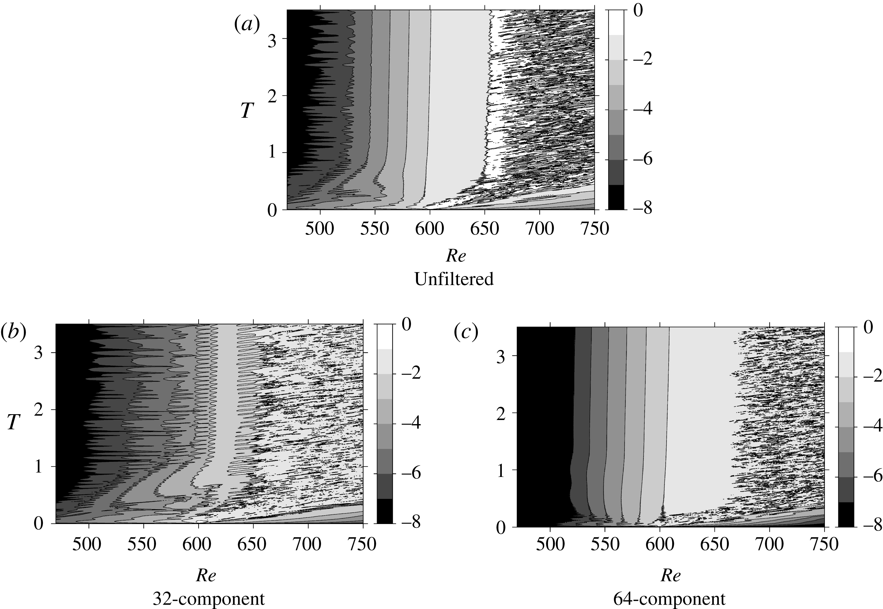
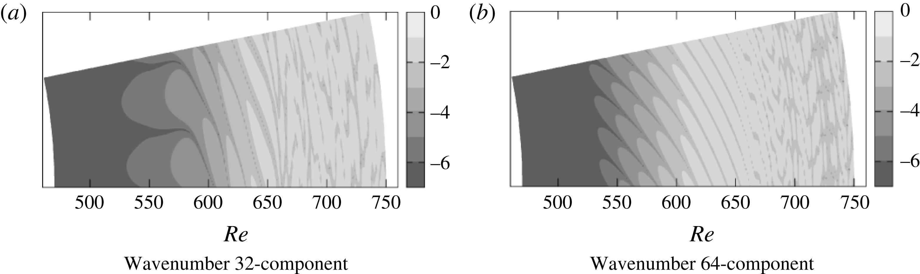
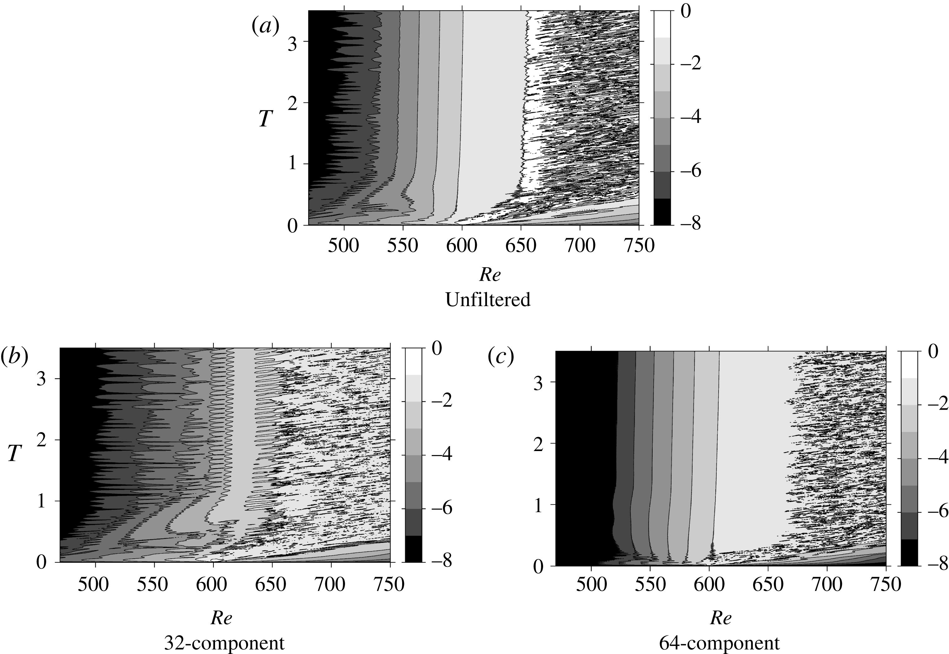
-component velocity fluctuation with a circumferential wavenumber of 32. Two waves, namely the wavenumber 32- and 64-components, can reside in the azimuthal direction in this computational domain. The results are shown in figure 10(a). The spatio-temporal diagram of
 $\log (v_{rms})$
in the case of
 $2\unicode[STIX]{x03C0}/32$
region computation is similar to those in the case of the
 $2\unicode[STIX]{x03C0}/68$
region computation shown in figure 7(a). The disturbance is first convected downstream, but gradually stops moving. After the flow field settles down, the starting point of the fully turbulent region can be found around
 $Re=650$
, as in figure 7. This demonstrates that the edge of the turbulent region does not change regardless of the size of the computational domain in the azimuthal direction,
 $2\unicode[STIX]{x03C0}/32$
or
 $2\unicode[STIX]{x03C0}/68$
. However, several differences can be found between the two diagrams. For example, the contour lines in the low-
 $Re$
region oscillate considerably only in the
 $2\unicode[STIX]{x03C0}/32$
case. In addition, the behaviour of the contour lines is different before the flow field settles down. Figures 10(b) and 10(c) show the diagrams for the wavenumber 32- and 64-components, respectively, extracted from figure 10(a) using a discrete Fourier transformation. Note that the flow field is excited by the wavenumber 32-component, so the 64-component is the harmonic of the forcing wavenumber. The diagram of the 64-component is quite similar to that of
 $2\unicode[STIX]{x03C0}/68$
region computation, while the diagram of the subharmonic 32-component (figure 10
b) is noisy at all times. This result shows that the noisy nature of the low-
 $Re$
field of figure 10(a) derives from the wavenumber 32-component. It can also be observed that the spatial growth rate of the 32-component is lower than that of the 64-component.
Spatio-temporal development of
 $\log (v_{rms})$
at
 $z=1.3$
for the
 $2\unicode[STIX]{x03C0}/32$
region computation case. (a) Original flow field including all wavenumber components. Filtered flow fields for (b) wavenumber 32-component and (c) wavenumber 64-component.
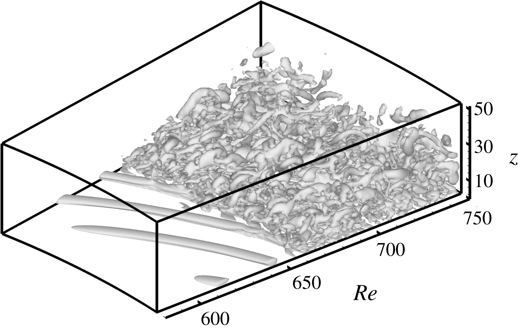
Isosurfaces of
 $\unicode[STIX]{x1D64C}=50$
at
 $T=3.5$
for the
 $2\unicode[STIX]{x03C0}/32$
region computation case.
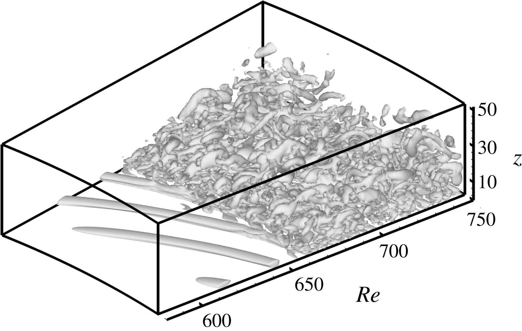
Vortical structures at
 $T=3.5$
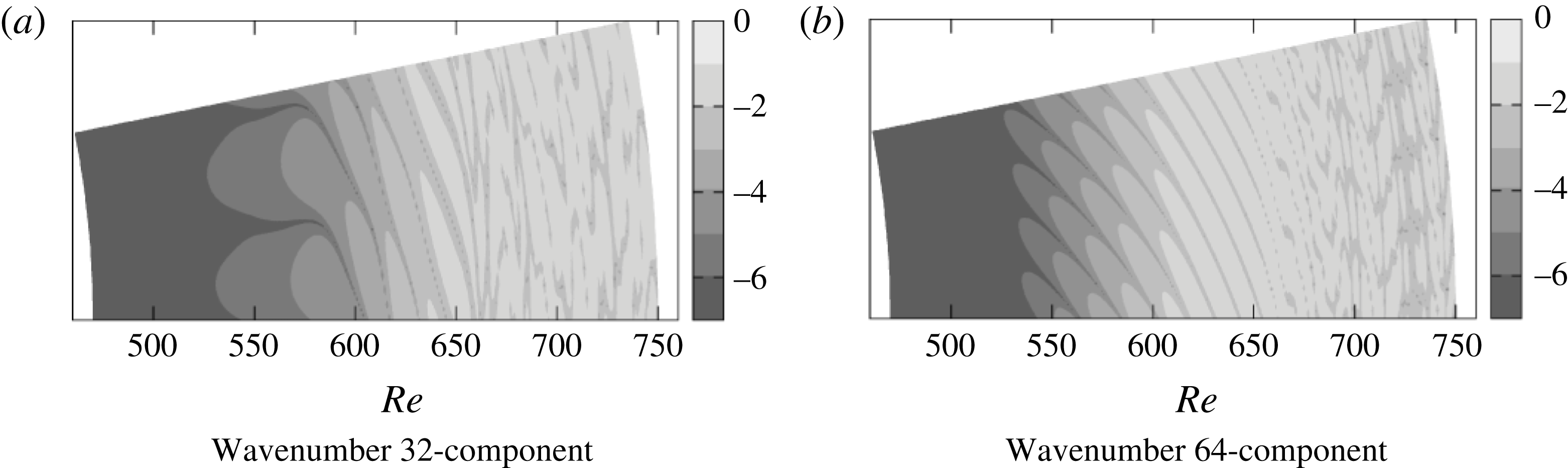
are shown in figure 11. Two spiral vortices can be clearly observed on the upstream side of the turbulent region in the original flow field. It is obvious that the flow field is governed by the 64-component, although it is the 32-component that was introduced into the flow field. Figure 12 shows the colour maps of
 $\text{log}|v|$
corresponding to each wavenumber component at
 $T=3.5$
, which is the azimuthal component of velocity fluctuation, at
 $z=1.3$
and
 $T=3.5$
. Because the absolute value of
 $v$
is shown, one spiral vortex appears as two-finger-like patterns in figure 12. In the
 $Re=600{-}660$
region of figure 12(a), which is the 32-component field, a two-finger-like pattern corresponding to the single spiral vortex can be observed. In contrast, in figure 12(b), which is the 64-component field, a four-finger-like pattern can be observed for a wide range of
 $Re=530{-}660$
.
Colour maps of
 $\text{log}|v|$
at
 $z=1.3$
and
 $T=3.5$
: (a) bandpass filtered by 32-component and (b) filtered by 64-component.
Frequency spectra of
 $v$
at
 $z=1.3$
and
 $Re=610$
, for
 $T=0.5{-}3.5$
.
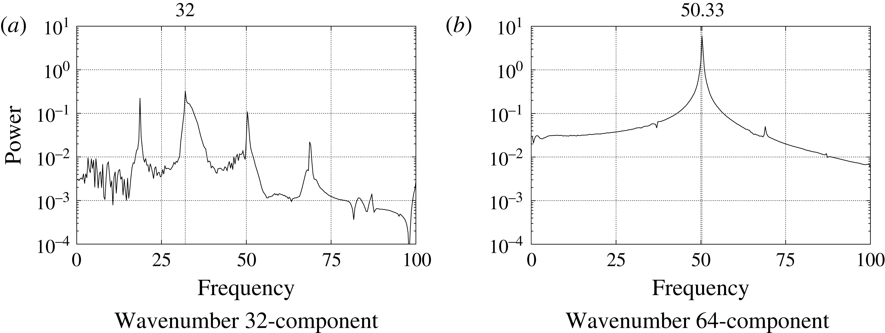
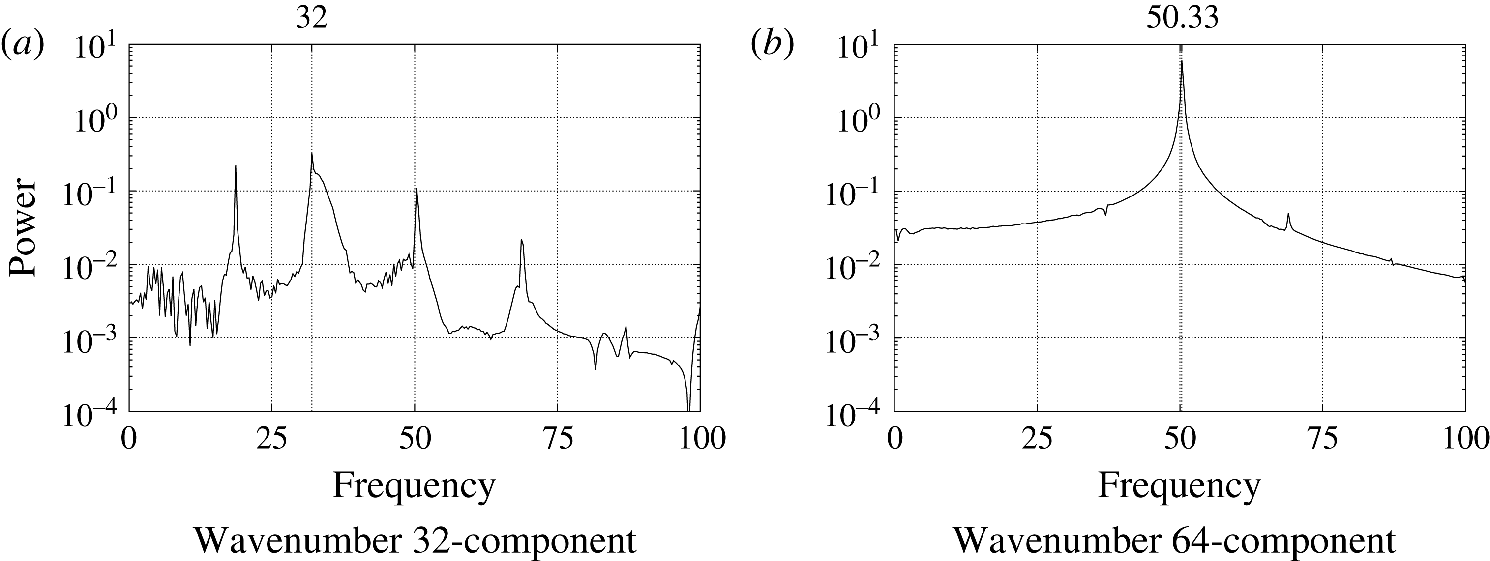
Figure 13 shows the temporal power spectra of azimuthal velocity for wavenumber 32- and 64-components, measured at
 $z=1.3$
and
 $Re=610$
. The data are from
 $T=0.5{-}3.5$
. The wavenumber 64-component has the frequency of 50.33, which is close to the frequency of the wavenumber 68-component in the
 $2\unicode[STIX]{x03C0}/68$
region computation. Because the values of the wavenumber and the frequency do not match, the 64 spiral vortices are travelling. On the other hand, the wavenumber 32-component peaks at the frequency of 32, indicating that it is stationary. The 32 spiral vortices in figure 12(a) have the same characteristics as spiral vortices found in the experiments. It should be noted that the power of the 32-component is an order of magnitude lower than that of the 64-component, which shows that the flow field is dominated by the travelling mode 64-component, which grows by the global instability.
3.3 Self-sustained system
In our computations, although the disturbance is given only at the start (
 $T<0.06$
), the flow field is self-sustained. It is therefore likely that a vibration source is present somewhere in the flow field. From a theoretical point of view, it is believed that the upstream spiral pattern is maintained by a stationary front of elephant global modes located at the transition radius from local convective to absolute instabilities, around
 $Re=507$
, when the external forcing is absent. Pier (Reference Pier2007) showed that, if localized periodic forcing is applied in the convectively unstable region, the naturally selected nonlinear global mode can be suppressed and replaced by the incoming finite-amplitude perturbations. Appelquist et al. (Reference Appelquist, Schlatter, Alfredsson and Lingwood2016b
) suggested that the global nonlinear flow is governed by the absolute instability properties at
 $Re=582.8$
, not 507, and the frequency of the absolute instability mode is triggered by the presence of downstream turbulence. In this section, the relation between the upstream velocity fluctuations at
 $Re<582.8$
, which are the spiral vortices, and the downstream turbulent region at
 $Re>650$
is investigated. The search for the location of the vibration source of the self-sustained structure of the rotating disk is pursued, and its relation to the elephant mode is discussed. We attempt to remove the turbulent region by two different methods, which will be explained later. The flow field at
 $T=5$
of the
 $2\unicode[STIX]{x03C0}/68$
case, where 68 spiral vortices are present, is used as the target for the investigation.
Time variation of sponge function
 $\unicode[STIX]{x1D706}$
.
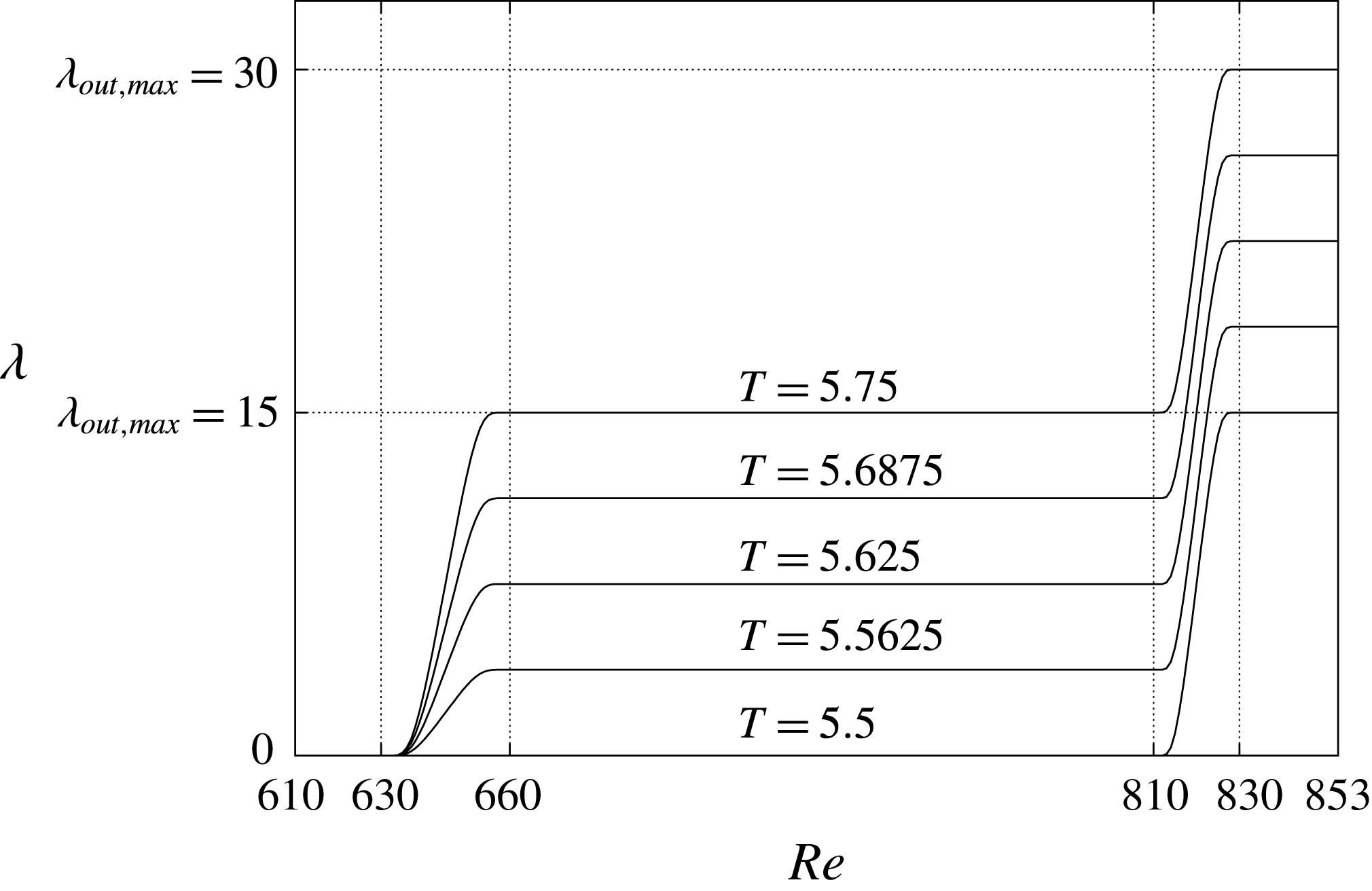
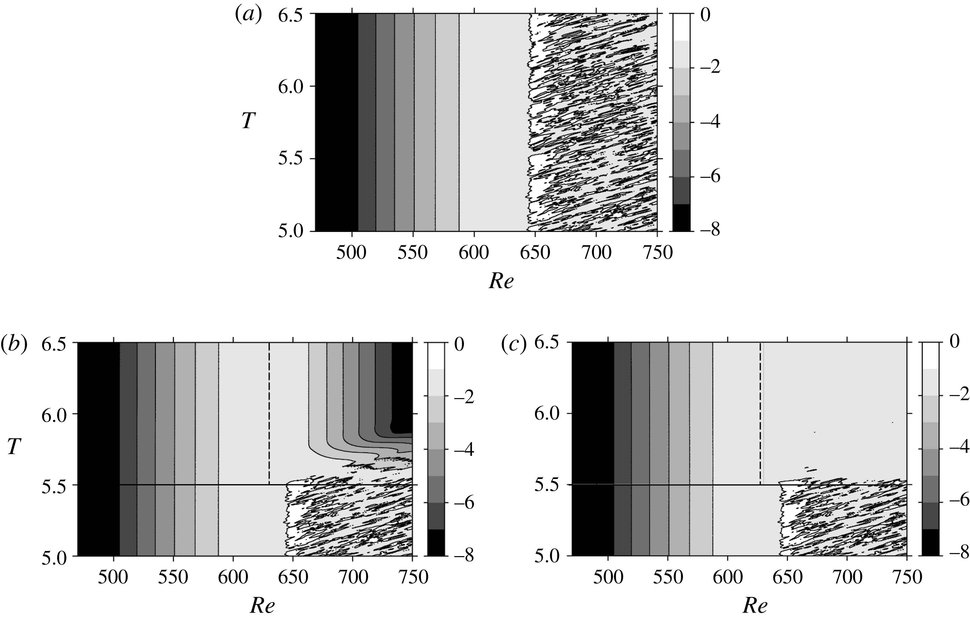
In the first attempt, the velocity fluctuations downstream of
 $Re=630$
are artificially damped by gradually changing the intensity of the sponge function
 $\unicode[STIX]{x1D706}$
in (2.14) from
 $T=5.5$
until
 $T=5.75$
, as shown in figure 14. The gradual change is intended to avert the impact of the abrupt change in the flow field. The original starting point of the sponge region was
 $Re=810$
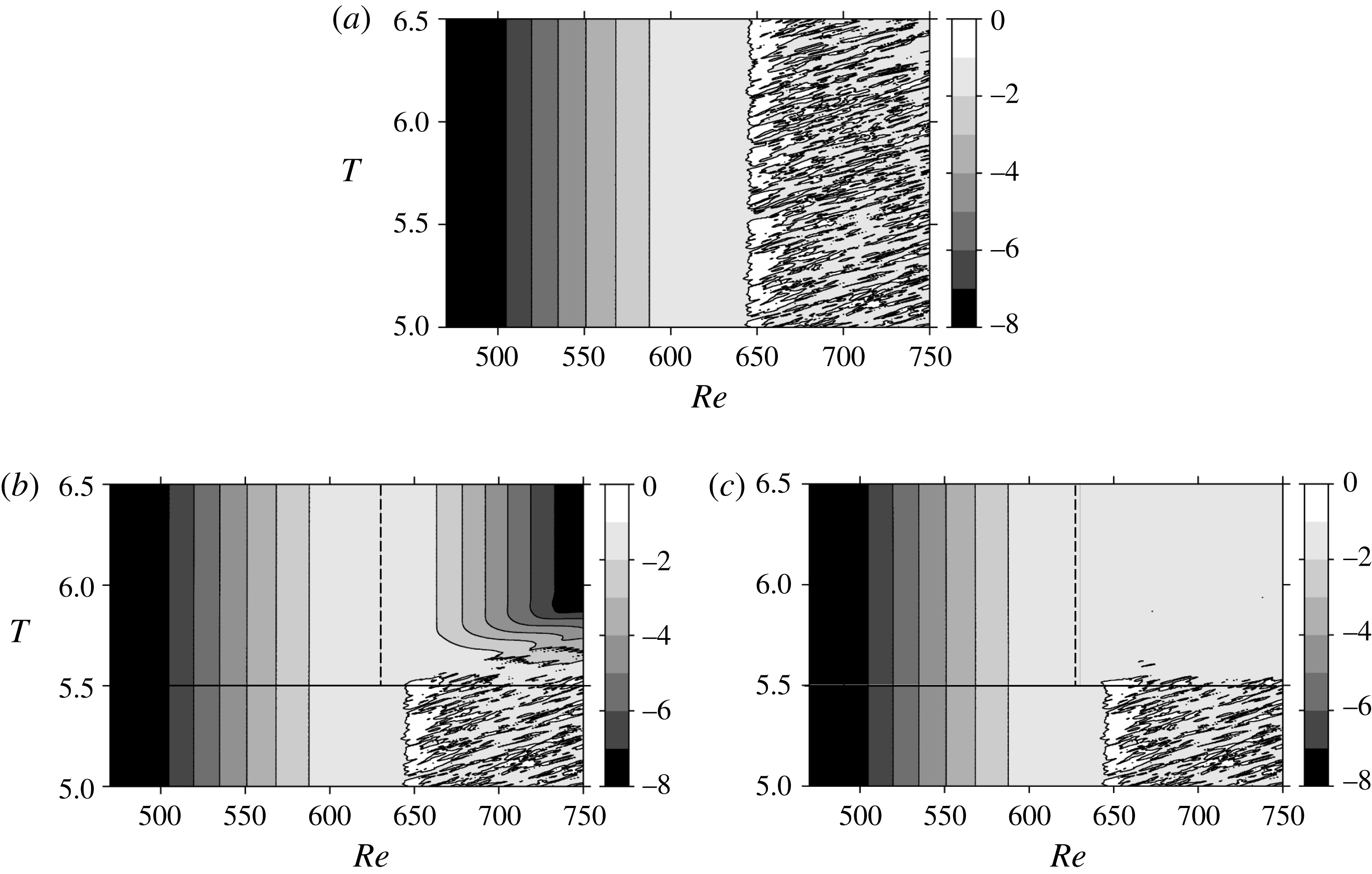
. The result is shown in figure 15(b). The reference case without any damping schemes is also shown in figure 15(a) for comparison. The turbulent region that existed in the
 $Re>645$
region has been effectively damped by extending the sponge region inward to
 $Re=630$
. In addition, the velocity fluctuation distribution becomes steady at around
 $T=5.8$
. It is obvious that removing the downstream turbulent region had a small effect on the flow field upstream of
 $Re<590$
.
In the second attempt, the turbulent region in
 $Re>645$
is removed in a milder way. A symmetric boundary condition,
 $\unicode[STIX]{x2202}(\tilde{U} +\tilde{u} )/\unicode[STIX]{x2202}z=0$
,
 $\unicode[STIX]{x2202}(\tilde{V}+\tilde{v})/\unicode[STIX]{x2202}z=0$
and
 $(\tilde{W}+\tilde{w})=0$
, i.e. the slip condition, is applied at the wall for the
 $Re>630$
region. The result shown in figure 15(c) indicates that this is also a very effective way to suppress turbulence. Unlike the method using the extended sponge region, the velocity fluctuation is not forced to damp downstream, so it nearly keeps its strength until the end of the computational region. As in the first attempt, removing the downstream turbulent region had a surprisingly small effect on the flow field upstream of
 $Re<590$
. Viaud, Serre & Chomaz (Reference Viaud, Serre and Chomaz2008) observed a nonlinear self-sustained mode in a source–sink flow between two rotating disks. The spiral vortices were sustained without downstream turbulence, which is similar to this study. They pointed out that an elephant mode arising at the upstream boundary of the absolute domain plays the role of a wavemaker triggering a saturated wave downstream whose frequency is determined at the local absolute frequency at this boundary.
Spatio-temporal development of
 $\log (v_{rms})$
at
 $z=1.3$
for (a) the reference case without any damping schemes, (b) the damping case with an expanded sponge region and (c) with a slip condition. The black solid line in (b,c) indicates the starting point of the expanded sponge region and the slip boundary condition region, respectively. The black dashed line in (b,c) divides the sponge region, or the slip boundary region from the normal calculation region.
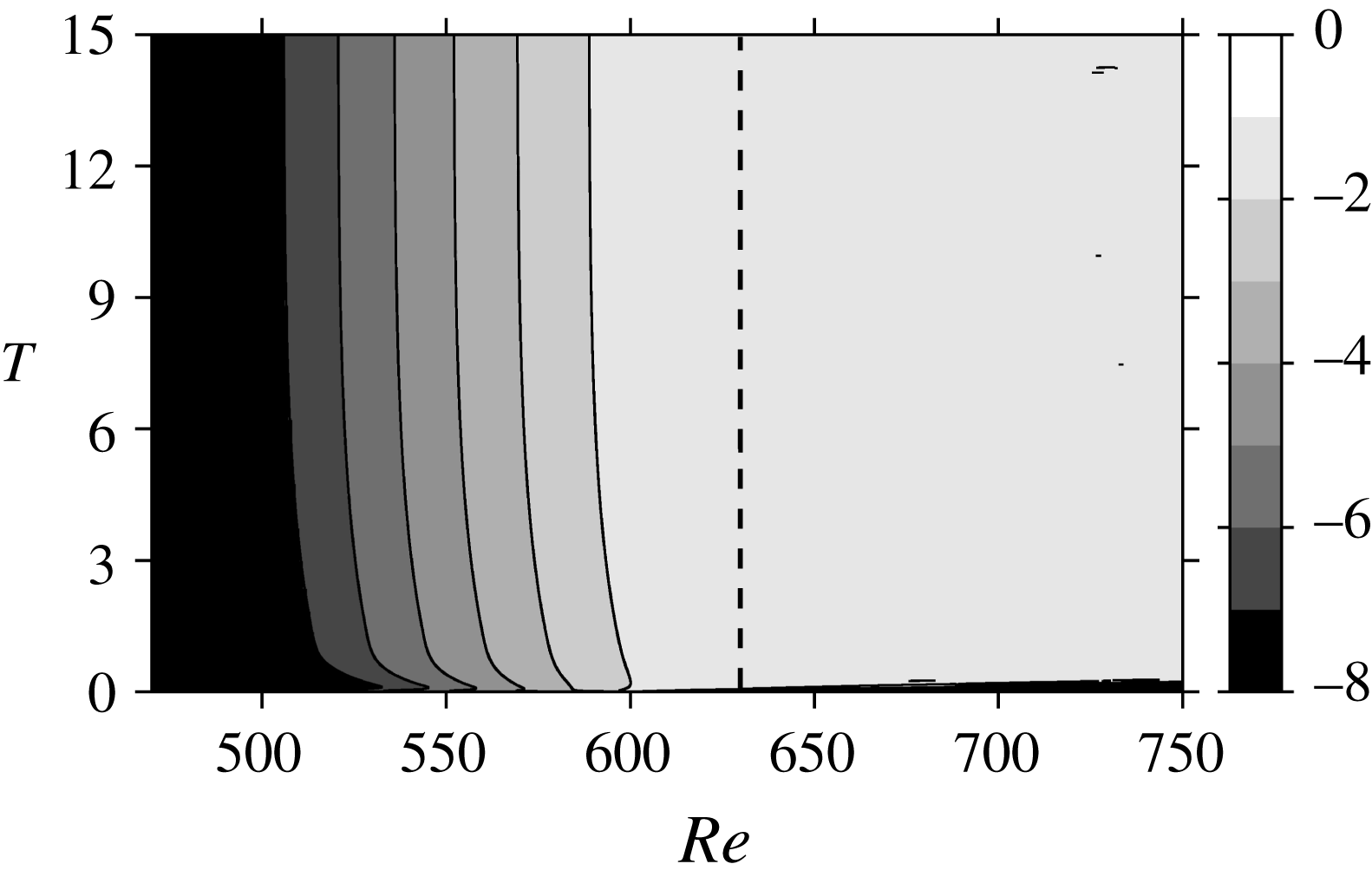
Spatio-temporal development of
 $\log (v_{rms})$
at
 $z=1.3$
when the slip condition is applied from the beginning of the computation,
 $T=0$
. The black dashed line divides the slip boundary region from the normal calculation region.
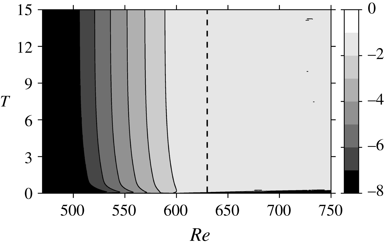
In order to clarify the effect of downstream turbulence on the upstream global mode, we performed an additional simulation in which the slip condition was applied from the beginning of the computation to the region of
 $Re>630$
. The maximum amplitude of initial disturbance,
 $w_{a,max}$
, was lowered to
 $0.005V$
so that turbulent transition would not take place. Other conditions are the same as the ordinary mesh
 $2\unicode[STIX]{x03C0}/68$
computation in table 1. The result is shown in figure 16. The initial disturbance is convected downstream and away from the computational domain without generating a turbulent region. Meanwhile, velocity fluctuations grow in the globally unstable region. It clearly shows that the velocity fluctuation field in the upstream region is sustained regardless of the presence of downstream turbulence. Also, the spatial variations of the azimuthal velocity fluctuation intensity,
 $v_{rms}$
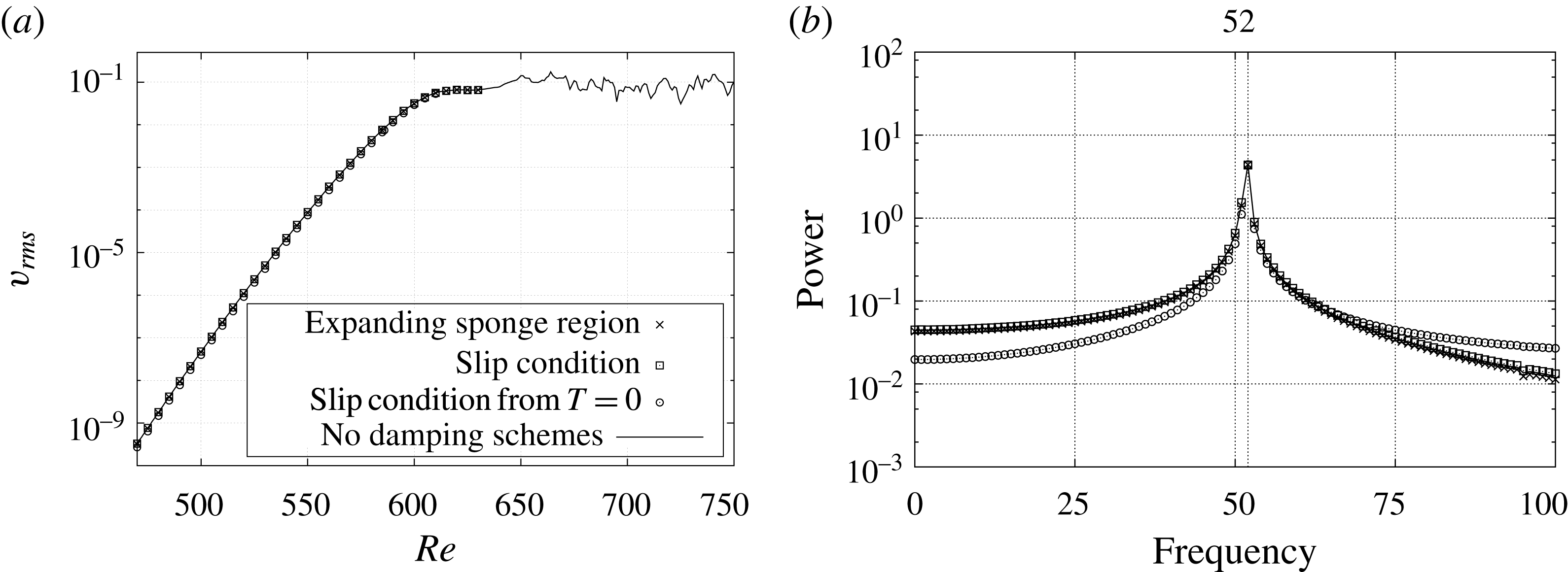
, after the flow field has reached the steady state, are compared in figure 17(a). The crosses and squares correspond to the final data at
 $T=6.5$
in figure 15(b,c). The original flow field without any damping schemes is also shown by a solid line in figure 15(a). A fully developed turbulent region is observed as a fluctuating part around
 $v_{rms}\approx 0.1$
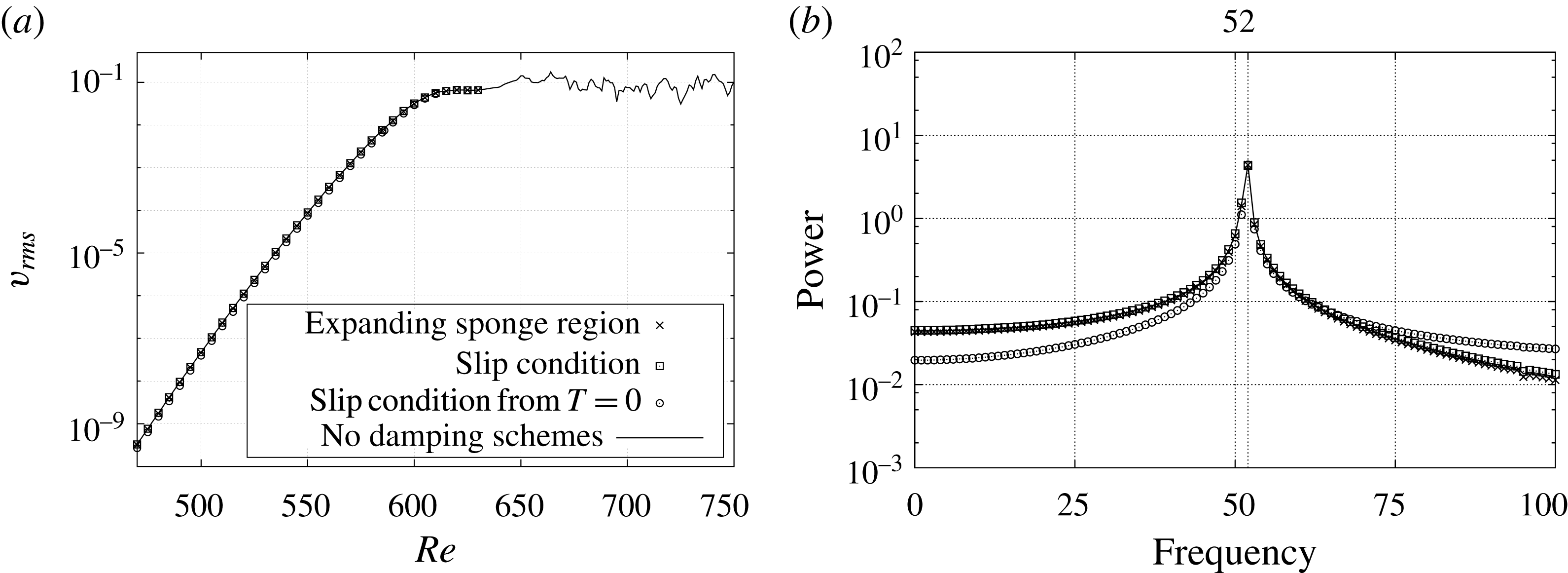
in figure 17(a). All these results are identical to the case when the slip condition is applied from the beginning of the computation. Also, figure 17(b) shows that the temporal power spectra of the azimuthal velocities have the same peak frequency of 52, which is the frequency of the travelling global mode of wavenumber 68-component. These results indicate that the origin of upstream global mode velocity fluctuations cannot be attributed to the turbulent field downstream.
Comparison of the flow fields at the steady state: (a) r.m.s. values of azimuthal velocity fluctuation
 $v_{rms}$
in the
 $z=1.3$
plane at
 $T=6.5$
; (b) frequency spectra of
 $v$
at
 $z=1.3$
and
 $Re=610$
calculated over the last rotation. The crosses indicate when the sponge region is placed in
 $Re>630$
region after
 $T=5.5$
, and the squares indicate when the slip boundary condition is applied instead. The data at
 $T=15$
when the slip condition is used from
 $T=0$
are also shown by circles. The reference case without any damping schemes is shown by a solid line.
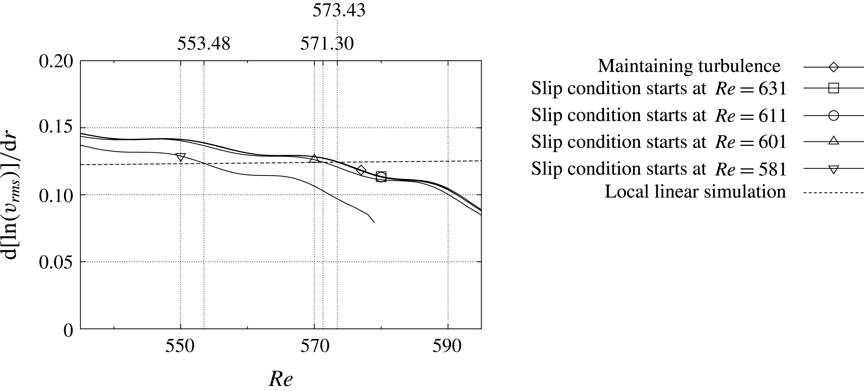
Spatial growth rate of
 $v_{rms}$
for each slip condition case at
 $T=7$
. The dashed line shows the result of local linear simulation.
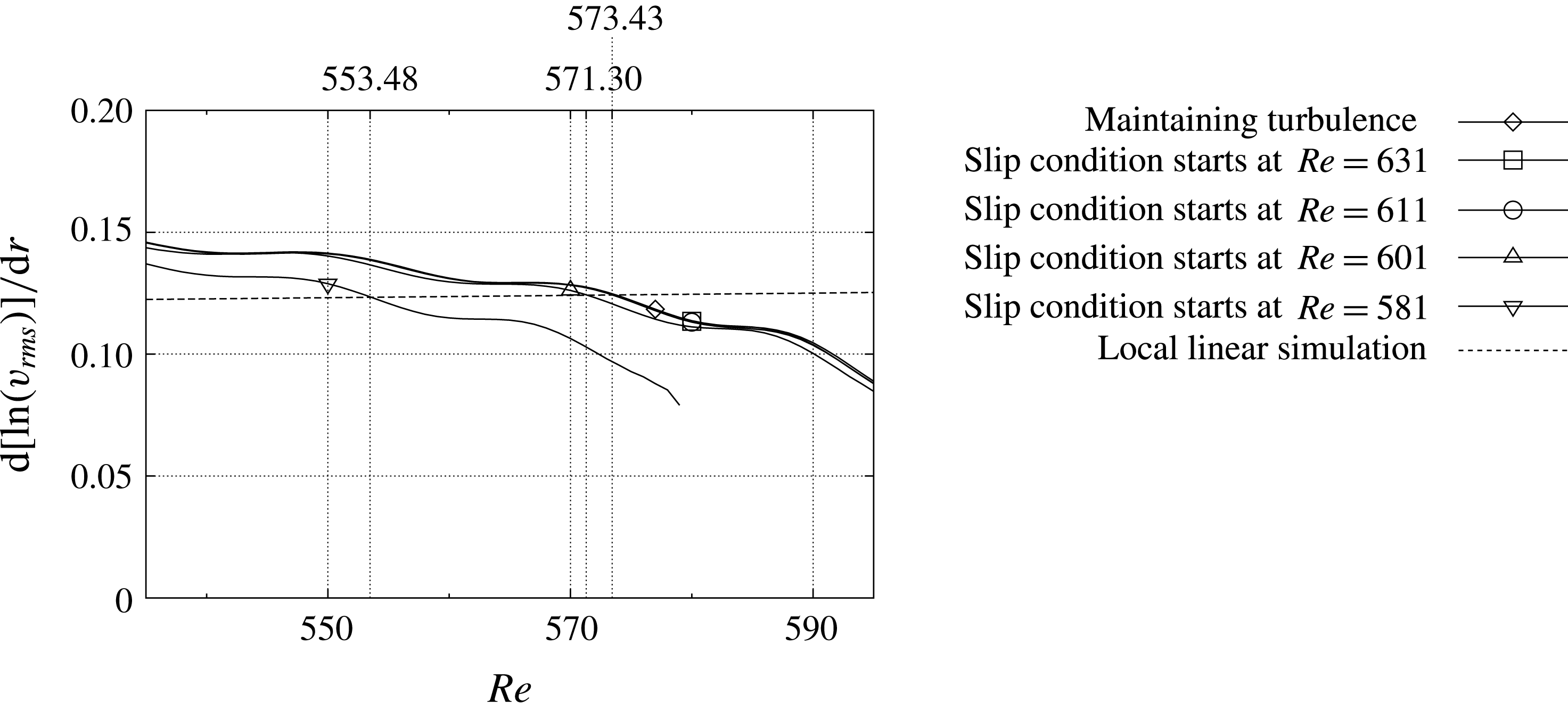
The relation between the upstream spiral structures and the downstream elephant mode is examined in detail by changing the starting point of the area where the slip condition is applied. Figure 18 shows the spatial growth rate of
 $v_{rms}$
in the radial direction at
 $T=7$
, when the slip condition is applied after
 $T=5.5$
to the region of
 $Re>630$
,
 $Re>610$
,
 $Re>600$
or
 $Re>580$
, and the turbulence is maintained. The result of linear simulation based on the parallel-flow assumption is also shown in figure 18. In all cases, the growth rates of azimuthal velocity fluctuations monotonically decrease as the Reynolds number increases and fall below that of the local linear simulation value. The point intersecting the local linear simulation result is at
 $Re^{nl}=573.43$
when the downstream turbulence is maintained without the damping schemes, and for the cases when the slip condition starts at
 $Re=611$
or 631. The curve shifts downward and the intersection moves to
 $Re^{nl}=571.30$
or 553.48 when the slip condition starts further upstream. The flow field is divided by this intersecting point into the upstream linear region and the downstream nonlinear region. It should be noted here that these values of
 $Re^{nl}$
are almost independent of time except for a short period right after the initial perturbation was added, whose reason is because strong perturbations were added to quickly obtain a steady state.
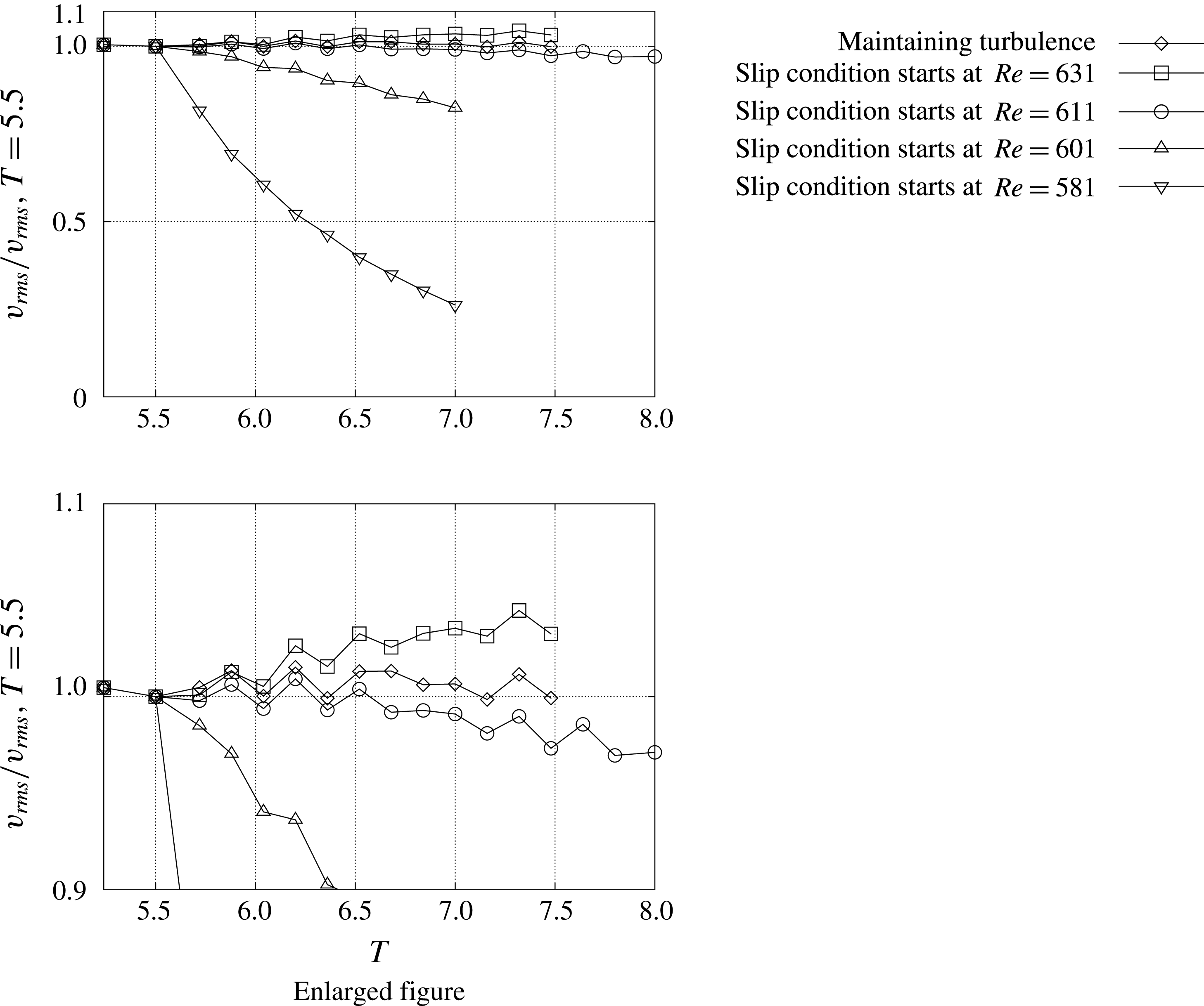
Temporal development of
 $v_{rms}$
for each slip condition case at
 $Re=560$
. All the profiles are normalized by the r.m.s. value at
 $z=1.3$
and
 $T=5.5$
.
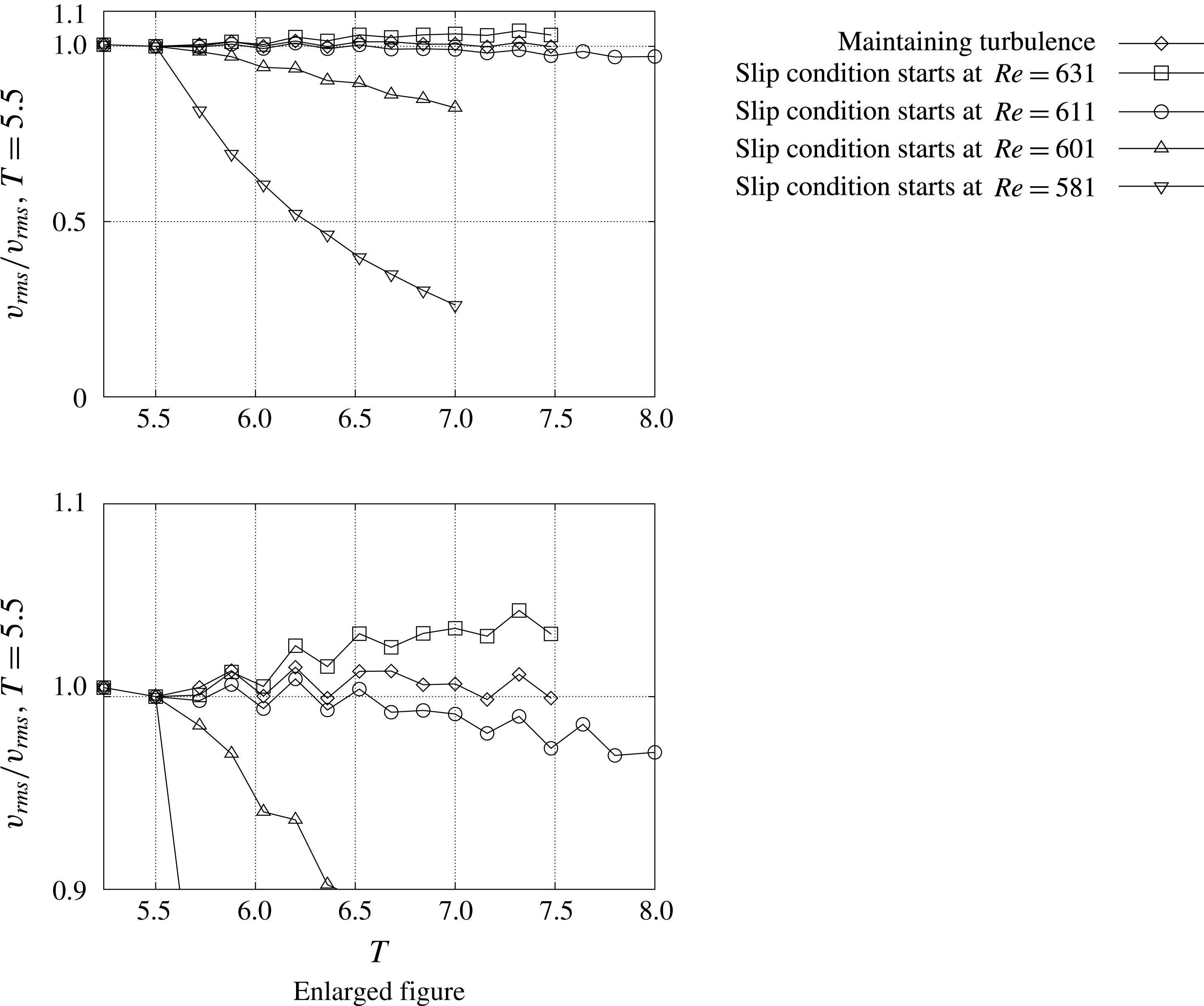
The temporal developments of
 $v_{rms}$
at
 $Re=560$
and
 $z=1.3$
changing the location where the slip condition starts are shown in figure 19. The data up to
 $T=8$
for the case when the slip condition starts at
 $Re=611$
are shown. The r.m.s. values at
 $T=5.5$
are used to normalize the profiles. When the turbulent region is sustained, the r.m.s. value stays at around the value of 1.0. A similar result is found for the case when the slip condition starts at
 $Re=631$
, though the r.m.s. value slightly rises with time. However, when the slip condition starts at
 $Re=611$
, 601 or 581, the r.m.s. values decrease with time, showing that the velocity fluctuations cannot be maintained under these conditions.
Pier et al. (Reference Pier, Huerre, Chomaz and Couairon1998) identified a stationary front of the elephant mode, which was referred to as the steep global mode in the literature, as the upstream boundary of the absolutely unstable domain in the context of the supercritical complex Ginzburg–Landau equation with coefficients slowly varying in space for a doubly infinite domain. As mentioned above, Appelquist et al. (Reference Appelquist, Schlatter, Alfredsson and Lingwood2016b
) deduced the critical Reynolds number for the global nonlinear modes in rotating-disk flows,
 $Re^{cg}=582.8$
, from the comparison of the growth rates in their nonlinear simulations and the local theory. Also, Viaud, Serre & Chomaz (Reference Viaud, Serre and Chomaz2011) observed a direct transition to turbulence through an elephant global mode cascade in a double-facing-disks configuration, in which the primary stationary front was already nonlinearly and globally unstable when it saturated. However, in our present research, except for the
 $Re=631$
case, the stationary front of elephant global modes cannot be present because the velocity fluctuations decrease with time. When the turbulence is maintained or the slip condition starts at
 $Re=631$
, the elephant mode arises at around
 $Re=573.4$
, which is given as a convergent value of
 $Re^{nl}$
for
 $T\rightarrow \infty$
. Our results in figures 18 and 19 also suggest that the self-sustained system is not always formed even if the nonlinearity becomes predominant in the globally unstable region. And the fact that the flow field cannot be sustained when the slip region appears upstream of
 $Re=611$
strongly indicates that the region of
 $611\leqslant Re<631$
, just upstream of the fully turbulent region, is necessary for the global mode velocity fluctuation to self-sustain itself. Consequently, we suggest that the source of vibration for the global instability, i.e. the vibration source, exists between
 $Re=611$
and
 $Re=631$
, and not at the location of the stationary front of the elephant global modes.
4 Conclusions
Direct numerical simulations were performed to investigate the role of the turbulent region on the self-sustaining mechanism of the spiral vortex structures of rotating-disk flows. Two computational domains with different azimuthal sizes,
 $2\unicode[STIX]{x03C0}/68$
and
 $2\unicode[STIX]{x03C0}/32$
, were computed. A disturbance was given in the form of a wall-normal short-duration suction and blowing at
 $Re=598{-}602$
, which was in the globally unstable region. The azimuthal wavenumber of the disturbance was chosen so that it matched the azimuthal wavenumber of the computational domain, and relatively large amplitude was given as a disturbance to quickly establish a wavy structure in the flow field.
When the azimuthal size of the computational domain was
 $2\unicode[STIX]{x03C0}/68$
, our flow field was in good agreement with the numerical results of Appelquist et al. (Reference Appelquist, Schlatter, Alfredsson and Lingwood2016b
). The disturbance grew while flowing down in the radial direction, and a turbulent region appeared at around
 $Re=640{-}650$
. Travelling spiral vortices were also formed in the
 $Re=590{-}640$
region, which was upstream of the turbulent region.
In the computation of a wider computational domain of
 $2\unicode[STIX]{x03C0}/32$
, the flow field was investigated by extracting the wavenumber 32- and 64-components. The pattern of the wavenumber 64-component was quite similar to the pattern found in the narrower domain case of
 $2\unicode[STIX]{x03C0}/68$
. Travelling spiral vortices of the 64-component were found to be much stronger and dominant compared to the 32-component.
In order to clarify the role of the turbulent region, the velocity fluctuations in that region were artificially suppressed after the flow field of
 $2\unicode[STIX]{x03C0}/68$
reached a steady state. Three methods were tested. As the first method, the velocity fluctuations downstream of
 $Re>630$
were damped using the sponge region. The turbulent region, which existed outside
 $Re=640{-}650$
, completely disappeared by the damping, and the velocity fluctuations were attenuated by the action. However, the flow field upstream of
 $Re<590$
showed no difference. As the second method, a slip condition was applied at the wall for
 $Re>630$
. In this case, the turbulent region disappeared, but the velocity fluctuations did not attenuate as in the former case, and the amplitude stayed almost constant for the entire
 $Re\leqq 630$
region as a result of the action. As the third method, a slip condition was applied for the region of
 $Re>630$
from the beginning of the computation and the amplitude of initial disturbance was lowered so that turbulence would not be generated. It was shown that the flow field would become globally unstable without the presence of the turbulent region. The results suggested that the downstream turbulent region was dispensable for the self-sustaining mechanism.
If the outer boundary of the computation was the source of the vibration, the sponge region would have blocked the disturbances travelling upstream in the first case, while in the second case, the disturbances could easily travel through the slip region. The fact that the flow field upstream of
 $Re<590$
was not affected by the control implied that the outer boundary was unlikely to be the source of the vibration.
The starting point to apply the slip condition was changed in order to investigate the existence and the location of the vibration source for the velocity fluctuations which grew by the global instability. When the slip condition was applied at
 $Re>610$
,
 $Re>600$
or
 $Re>580$
, the flow fields could not be sustained by the global instability any more. The results indicated that the location of the vibration source was located between
 $Re=611$
and
 $Re=631$
.