



Nomenclature
- ACM
-
adaptive coding and modulation
- AI
-
artificial intelligence
- ARQ
-
automatic repeat request
- AZ
-
azimuth
- CNN
-
convolutional neural networks
- DRL
-
deep reinforcement learning
- EL
-
elevation
- XGBoost
-
Xtreme Gradient Boosting
- FT
-
fault tolerant
- FT-TSR
-
fault-tolerant tracking signal receiver
- FSO
-
free space optical
- GWO
-
grey wolf optimised
- GS
-
ground station
- KF
-
Kalman filter
- KNN
-
K-nearest neighbors
- LEO
-
low earth orbit
- LNA
-
low-noise amplifier
- ML
-
machine learning
- ML-TSR
-
machine learning tracking signal receiver
- MDP
-
Markov decision process
- MSE
-
mean squared error
- PSO
-
particle swarm optimisation
- PPO
-
proximal policy optimisation
- RF
-
radio frequency
- RSSI
-
receiver signal strength indicator
- RSL
-
receiver signal level
- RMSE
-
root mean squared error
- SSO
-
sun-synchronous orbit
- SL-LSTM
-
supervised long short-term memory
- SVM
-
support vector machines
- TWTA
-
traveling wave tube amplifiers
1.0 Introduction
In low earth orbit (LEO) and sun-synchronous orbit (SSO) missions, ensuring reliable communication is a challenge due to very short passes and severe operational environment requirements. In the literature, the reliability and efficiency of the communications are provided by classical multi-layer link mechanisms, including adaptive coding and modulation (ACM) [Reference Caire and Kumar1, Reference Örmeci, Liu, Goeckel and Wesel2], received signal strength indicator (RSSI) monitoring [Reference Gongora-Torres, Vargas-Rosales, Aragón-Zavala and Villalpando-Hernandez3], automatic repeat request (ARQ) [Reference Le and Pham4] and hardware redundancy [Reference Lohmeyer, Aniceto and Cahoy5] in critical subsystems for the physical layer, such as dual transponders, traveling wave tube amplifiers (TWTAs) and antennas in hot- or cold-standby configurations, as well as advanced signal impairment mitigation techniques such as Doppler shift compensation and polarisation management approaches for satellite communications [Reference Nasri, BAB, Saiah, Hamed and Adnane6].
Furthermore, leveraging recent advanced approaches, numerous research works have investigated the integration of artificial intelligence (AI) across most satellite subsystems such as on-board image processing (cloud detection, image filtering, etc.), attitude control, autonomous navigation and thruster management, as well as radio frequency (RF) communication subsystems, including transponders, amplifiers and patch antennas [Reference Fontanesi, Ortiz and Lagunas7–Reference Hassan and Hassan10]. The authors in Ref. [Reference El Hariry, Cini, Mellone and Balossino11] apply deep reinforcement learning (DRL) through a proximal policy optimisation (PPO) to a Markov decision process (MDP) model to learn fault-tolerant (FT) satellite attitude control, capable of executing large manoeuvres with standard-compliant precision despite actuator failure. In addition, the authors in Refs [Reference Loettgen, Ceriotti, Aragon-Camarasa and Worrall12, Reference Ma, Wang, Yang, Wang, Tang and Ackland13] demonstrate that DRL) enables the optimisation of attitude control laws, which allows improving pointing robustness against uncertainties, noise and perturbations. These advances may ultimately contribute to improving the quality of pointing and tracking manoeuvres, including for non-cooperative targets, within architectures combining onboard control and ground segment supervision. However, these approaches present certain limitations where they only handle limited failures and require significant computational power not supported by on-board limited resources.
Consequently, these limitations can cause, in practice, misalignment between the satellite and the ground segment, affecting communication and tracking. In this context, Ref. [Reference Huang, Ji, Zhai, Yang and Yang14] proposes a supervised long short-term memory (SL-LSTM) model to predict navigation satellite clock bias, capturing both cyclic and random components to improve temporal accuracy over medium to long durations. Although high performing, the model depends heavily on high-quality historical data that can be sensitive to anomalies, which requires substantial computational resources for training and updating across large satellite constellations. In a similar context Ref. [Reference Alam, Yusof and Faudzi15] presents a dual-band (X/Ku) microstrip patch antenna whose resonance frequencies are predicted by machine learning (ML) models, including regression and convolutional neural networks (CNNs). Similarly, Ref. [Reference Maharjan and Kim16] shows that the use of predictive models, such as neural networks or support vector machines (SVMs), allows for real-time correction of beam-pointing errors in satellite-to-ground free space optical (FSO) links. However, these approaches remain dependent on data and simulated scenarios, which may limit their reliability under practical operational conditions.
The validity of these methods is affected by the quality of the ground segment infrastructure, which constitutes the overall framework for anomaly detection, pointing error correction and the guarantee of reliable communications. In line with these works, the present paper focuses specifically on the ground segment side. The ground station (GS) faces several challenges related to precise satellite tracking, where these difficulties can be observed, analysed and addressed operationally. To this end, recent works focus on automatic antenna tracking strategies where the beacon tracking strategy continuously points the antenna by maximising received power or following the carrier phase of a dedicated signal using Kalman filter (KF) loops. Such a solution compensates for Doppler shifts and geometric variations [Reference Periyapatna, Murali, Basavaraju, Bagali, Goparaju and Purohith17–Reference Roy, Nagasekhar, Saha, Mane, Padmavathy, Umadevi and Kumar19], so, they ensure robust real-time pointing. Nevertheless, the performance degrades when the beacon’s carrier-to-noise density ratio (C/N0) becomes low.
In this context, the precise estimation of azimuth, elevation and Doppler shift remains essential. In Ref. [Reference Bensikaddour, Nasri, Hamed, Kaddouri and Saiah20], these parameters are estimated using an open-source Python tool that relies on the Ephem library, then compared with measurements from the operational ALSAT-2 GS data. Experimental tests demonstrate that the developed solution enables reliable tracking. However, its accuracy depends heavily on the quality of received measurements and atmospheric conditions.
Although ML techniques are still under-exploited in the GS domain, the authors of Ref. [Reference Bensikaddour, Nasri, Bouchiba, Baba Hamed and Saiah21] proposed an intelligent solution for the ground acquisition of ALSAT-2 satellite telemetry. This approach applies the K-nearest neighbors (KNN) method to drive the polarisation device. It demonstrates that intelligent methods can be integrated to improve existing systems by introducing and proposing resilient hybrid frameworks for FT operation.
Our contribution extends the study detailed in Ref. [Reference Nasri, Saiah, Meghabber and Bouchiba22] by integrating ML into the previously established monopulse auto-tracking architecture using a particle swarm optimisation (PSO) algorithm for antenna pointing in the Oran’s GS. This article proposes the integration of ML into an FT monopulse system to supplement automatic control in the case of anomalous events. The study focuses on active components, specifically the low-noise amplifier (LNA), which, from our experience and feedback, can degrade progressively or fail completely so that it will affect the whole system performance. To manage these failures, a likelihood function is introduced, and its statistical parameters are optimised using the grey wolf optimised (GWO) algorithm. This function allows the system to automatically switch to machine learning tracking signal receiver (ML-TSR) control as soon as an anomaly is detected. ML-TSR, based on KNN, offers better performance than eXtreme Gradient Boosting (XGBoost) and decision trees.
The remainder of this paper is organised as follows: Section 2 presents the design and architecture of the proposed auto-tracking system, including the modeling of RF components (a case study of the LNA), the probabilistic decision algorithm, GWO-based optimisation and the ML models for auto-track prediction. Section 3 reports the experimental setup and evaluation results obtained through ALSAT-1B data, and Section 4 concludes the paper.
2.0 Design and architecture of the proposed auto-tracking system
In this section, we present the fault-tolerant tracking signal receiver (FT-TSR) approach, based on ML (see Fig. 1, dashed area), designed to take over from the monopulse auto-track system in the event of an LNA failure. At the start of a pass, the antenna operates in the S or X band, with measurements computed by the simplified general perturbations model 4 (SGP4) propagator, which provides the
 $\boldsymbol{EL}$
and
 $\boldsymbol{AZ}$
coordinates. When a predefined signal level threshold is exceeded, the auto-track system is activated, providing the coordinates
 $\boldsymbol{EL}'$
and
 $\boldsymbol{AZ}'$
, corresponding to nominal operation. In the case of a partial or total LNA failure, the likelihood function, whose statistical parameters are optimised using the GWO algorithm, detects the fault and automatically switches to the ML-TSR controller. The detailed operation of this function will be presented later.
Design of a fault detection scheme for monopulse auto-tracking.

Figure 1 Long description
A diagram of a fault detection scheme for monopulse auto-tracking. The diagram includes several components and processes. On the left, there is a satellite labeled ALSAT-1B, which is connected to a tracking signal receiver. The receiver is linked to two propagators labeled SGP4 Propagator, one directly and one through a decision point labeled SLevel < S0. The SGP4 Propagator provides TLE data to both the FT-TSR and ML-TSR systems. The FT-TSR system includes a likelihood function optimization process and outputs EL, AZ data to an S/X Band antenna. The ML-TSR system outputs EL, AZ data directly. The diagram shows the flow of data and the interaction between different components to ensure reliable communication in low earth orbit and sun-synchronous orbit missions.
2.1 Modeling of RF components: a case study on the LNA
The X-band chain of the monopulse system at the Oran station incorporates three identical amplifiers [Reference Nasri, Saiah, Meghabber and Bouchiba22] of reference AMFW-6S-07700850-50-N-R [23]. Their modeling is based on the manufacturer’s specifications in order to faithfully reproduce their performance (see Table 1).
To anticipate the effects of potential failures, it is essential to define a tolerance strategy for the LNA, particularly by considering the impact of a fault on the input impedance. The effective gain of the LNA depends on the impedance mismatch and can be expressed using the reflection coefficient
 ${{\Gamma }}$
, defined as
 \begin{align}{\boldsymbol{\Gamma }} = \frac{{{Z_{in}} - {Z_s}}}{{{Z_{in}} + {Z_s}}}\end{align}
with
 ${Z_{in}}$
being the input impedance of the LNA and
 ${Z_s}$
the source impedance (typically 50Ω). The corresponding gain loss in decibels is given by [Reference Pozar24]:
 \begin{align}\Delta \boldsymbol{G}({{{dB}}}) = 10{\textrm{log}}_{10}({1 - {{|{\boldsymbol{\Gamma }}|}^2}})\end{align}
Main specifications of the AMFW-6S-07700850-50-N-R amplifier

Table 1 Long description
A table with three columns and eight rows detailing the specifications of the AMFW-6S-07700850-50-N-R amplifier. The columns are labeled Parameter, Value, and Significance. Row 1: Parameter, Frequency band; Value, 7.70 – 8.50 GHz; Significance, Amplifier bandwidth. Row 2: Parameter, Gain; Value, ≥ 50 dB; Significance, Nominal gain. Row 3: Parameter, Gain flatness; Value, ± 1 dB; Significance, Frequency variation of gain. Row 4: Parameter, Gain vs temperature; Value, ± 5 dB; Significance, Thermal dependence. Row 5: Parameter, Noise factor; Value, 45 K max (40 K typ.); Significance, Added noise. Row 6: Parameter, P1dB output; Value, + 10 dBm min; Significance, Linearity limit. Row 7: Parameter, VSWR in/out; Value, ≤ 1.5:1; Significance, Impedance matching. Row 8: Parameter, Temperature; Value, -40 to +60 °C; Significance, Temperature rating.
For a given voltage standing wave ratio (VSWR), the reflection coefficient can be calculated as follows:
 \begin{align}\left| {\boldsymbol{\Gamma }} \right| = \frac{{{\textrm{VSWR}} - 1}}{{{\textrm{VSWR}} + 1}}\end{align}
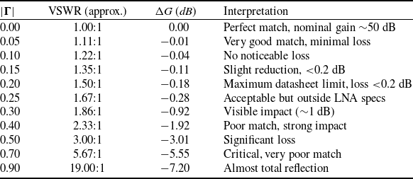
Table 2 illustrates the impact of the reflection coefficient
 $\left| {{\Gamma }} \right|$
on the LNA gain.
Impact of impedance matching on LNA gain

Table 2 Long description
A table with four columns and nine rows. The columns are labeled as follows: |Γ|, VSWR (approx.), ΔG (dB), and Interpretation. The rows present the following data: Row 1: |Γ|, 0.00; VSWR (approx.), 1.00:1; ΔG (dB), 0.00; Interpretation, Perfect match, nominal gain 50 dB. Row 2: |Γ|, 0.05; VSWR (approx.), 1.11:1; ΔG (dB), 0.01; Interpretation, Very good match, minimal loss. Row 3: |Γ|, 0.10; VSWR (approx.), 1.22:1; ΔG (dB), 0.04; Interpretation, No noticeable loss. Row 4: |Γ|, 0.15; VSWR (approx.), 1.35:1; ΔG (dB), 0.11; Interpretation, Slight reduction, <0.2 dB. Row 5: |Γ|, 0.20; VSWR (approx.), 1.50:1; ΔG (dB), 0.18; Interpretation, Maximum datasheet limit, loss <0.2 dB. Row 6: |Γ|, 0.25; VSWR (approx.), 1.67:1; ΔG (dB), 0.28; Interpretation, Acceptable but outside LNA specs. Row 7: |Γ|, 0.30; VSWR (approx.), 1.86:1; ΔG (dB), 0.92; Interpretation, Visible impact (1 dB). Row 8: |Γ|, 0.40; VSWR (approx.), 2.33:1; ΔG (dB), 1.92; Interpretation, Poor match, strong impact. Row 9: |Γ|, 0.50; VSWR (approx.), 3.00:1; ΔG (dB), 3.01; Interpretation, Significant loss. Row 10: |Γ|, 0.70; VSWR (approx.), 5.67:1; ΔG (dB), 5.55; Interpretation, Critical, very poor match. Row 11: |Γ|, 0.90; VSWR (approx.), 19.00:1; ΔG (dB), 7.20; Interpretation, Almost total reflection.
Assumption 1. Gain failure due to LNA mismatch (critical mission). A relevant interval for the failure assumption is defined by:
 \begin{align*}\left\{\! \begin{array}{l@{\quad}l}|\unicode{x1D71E} | \in[{0.25,{{\;}}0.40} [(\Delta \boldsymbol{G} \in [-\!1.92, - 0.28\,dB])\qquad\quad \textrm{Potential risk out of specification}.\\| \unicode{x1D71E} | \ge 0.40\;\;\Delta G\; \le - 1.92\;dB \qquad \qquad \qquad \qquad \textrm{Strict and valid failure assumption.}\end{array} \right.\end{align*}
2.2 The probabilistic decision algorithm
A probabilistic decision algorithm is employed to estimate the failure probability of the LNA component. The algorithm uses the outputs of the TSR as observations
 $\unicode{x1D71F}{\boldsymbol{G}_k}$
to compute the likelihood of a fault. The likelihood function is based on the measured reflection coefficient of magnitude
 ${\boldsymbol{x}_k} = \left| {{{\boldsymbol{\Gamma }}_k}} \right|$
. In the event of failure or degradation of one of the LNAs, the likelihood function automatically transfers control to the ML-TSR module, which relies on ML to maintain system reliability.
Remark 1. In the event of a failure or degradation of any of the three LNAs, the likelihood function automatically transfers control to the FT-TSR module, which relies on ML.
The gain loss can be expressed in terms of the reflection coefficient as:
 \begin{align}\unicode{x1D71F} {\boldsymbol{G}_k} = 10\,{\textrm{log}}_{10}\big({1 - {\boldsymbol{x}_k}^2}\big),\,{\boldsymbol{x}_k} = |{\boldsymbol{\Gamma}}|\end{align}
The likelihood of the measured gain variation
 $\unicode{x1D6E5} {G_k}$
under state
 ${H_{s(k)}}$
is modeled as a normal (Gaussian) distribution [Reference Casella and Berger25]:
 \begin{align}L({\unicode{x1D71F} {\boldsymbol{G}_k}|{H_{s(k)}}}) = \frac{1}{{\sqrt {2\pi \boldsymbol\sigma _{s(k)}^2} }}\exp\left({-\frac{{{{({\unicode{x1D71F} {\boldsymbol{G}_k} - {\boldsymbol\mu _{s(k)}}})}^2}}}{{2\boldsymbol\sigma _{s( k )}^2}}}\right)\end{align}
where
 ${\boldsymbol\mu _{s(k)}}$
and
 ${\boldsymbol\sigma _{s(k)}}$
are the mean and standard deviations assigned according to the state of the observation.
Assignment to observations. For each of the
 ${{\;}}{N_s}$
observation
 $\unicode{x1D71F}{\boldsymbol{G}_k}({k = 1, \ldots ,\,{N_s}})$
the corresponding parameters
 ${\boldsymbol\mu _{s(k)}}$
and
 ${\boldsymbol\sigma _{s(k)}}$
are assigned based on the associated state
 $s(k)$
, (0 for normal, 1 for faulty):

Note (for reference). If estimated classically from the measurements, the mean and variance for each state
 $i \in \left\{{0,1}\right\}$
would be:
 \begin{align}\left\{ {\begin{array}{*{20}{c}}{{\boldsymbol\mu _i} = \;\dfrac{1}{{{N_i}}}\mathop \sum \limits_{k = 1}^{{N_s}} {\textbf{1}_{\left\{ {s(k) = i} \right\}}}\unicode{x1D71F} {\boldsymbol{G}_k}\;\;\;\;\;\;\;\;\;\;\;\;\;\;\;\;\;\;\;\;\;\;}\\[9pt]{\boldsymbol\sigma _i^2 = \dfrac{1}{{{N_i} - 1}}\mathop \sum \limits_{k = 1}^{{N_s}} {\textbf{1}_{\left\{ {s(k) = i} \right\}}}{{(\unicode{x1D71F} {\boldsymbol{G}_k} - {\boldsymbol\mu _i})}^2}\;\;\;\;}\end{array}} \right.\end{align}
where:
-
•
 ${N_i}$
is the number of measurements corresponding to state
${{\;}}i$
.
-
•
${\textbf{1}_{\left\{ {s(k) = i} \right\}}}$
is the indicator function (
$1$
if measurement
$k$
belongs to state
$i$
,
$0$
otherwise).


Remark 2. The statistical parameters
 ${\boldsymbol\mu _0}$
,
 ${\boldsymbol\sigma _0},{\boldsymbol\mu _1}$
and
 ${\boldsymbol\sigma _1}$
of the likelihood models in Equation (5) are directly optimised using the GWO algorithm, rather than computed from classical sample estimates.
Remark 3. During fault detection, the likelihood function is evaluated solely as a statistical measure of consistency between the observed signal and the nominal model. No gradient computation (i.e. ∇L = 0) or search for a minimum/maximum is performed, and detection is based on a predefined threshold.
The likelihood ratio for each observation is computed as:
 \begin{align}\boldsymbol\varLambda({{\unicode{x1D71F}}{\boldsymbol{G}_{\boldsymbol{k}}}}) = \frac{{{{L}}( {{\unicode{x1D71F}}{\boldsymbol{G}_{{k}}}\,{{{H}}_1}} )}}{{{{L}}( {{\unicode{x1D71F}}{\boldsymbol{G}_{{k}}}\,{{{H}}_0}} )}} \lessgtr {{\eta }}\end{align}
Assumption 2 (decision rule). Each observation
 $\Delta {G_k}$
is evaluated independently. A fault is declared if
 $\boldsymbol\varLambda({\boldsymbol\Delta {\boldsymbol{G}_k}}) \gt \eta ,$
(assumption
 ${H_1}$
); otherwise, the system is considered to be in normal operation (
 ${H_0}$
).
Assumption 3 (measurement model). The measured reflection coefficient magnitude,
 ${\boldsymbol{x}_k} = \left| {{{\boldsymbol{\Gamma }}_k}} \right|$
, is modeled under two assumptions:
-
•
${H_0}$
(normal LNA):
${{\;}}{\boldsymbol{x}_k}$
is low and follows a Gaussian distribution with mean
${\boldsymbol\mu _0}$
and variance
$\boldsymbol\sigma _0^2$
. -
•
${H_1}$
(faulty LNA):
${x_k}$
is high and follows a Gaussian distribution with mean
${\boldsymbol\mu _1}$
and variance
$\boldsymbol\sigma _1^2$
.


2.3 Grey wolf optimisation
GWO is a nature-inspired metaheuristic mimicking grey wolf hunting behaviour and hierarchy [Reference Boualem26]. The three best solutions
 $\;\left( {\alpha ,{{\;}}\beta ,{{\;}}\delta } \right)$
guide the population. Wolf positions are updated iteratively using:
-
1. Coefficient vectors:
(8)such as
\begin{align}\left\{ {\begin{array}{*{20}{c}}{{\vec{A}} = 2.{\vec{a}}.\,{{{\vec{r}}}_1} - {\vec{a}}\;}\\{{\vec{C}} = 2.{{{\vec{r}}}_2}\;\;\;\;\;\;\;\;\;\;\;\;}\end{array}} \right.\end{align}
(9)where
\begin{align}{\vec{a}} = 2 - 2\;.\,{{n}}/{Max\_iter}\end{align}
${\vec r_1}$
,
${\vec r_2}$
$ \in \left[ {0,1} \right]$
are random vectors,
$n$
is the actual number of iterations and
$Max\_{iter}$
is the maximum number of iterations.
-
2. Distance to leaders:
(10)
\begin{align}\left\{ {\begin{array}{*{20}{c}}{{{{\vec{D}}}_{{\alpha }}} = \left| {{\vec{C}}.\,{{{\vec{X}}}_{{\alpha }}} - {{{\vec{X}}}_{{j}}}} \right|}\\[5pt]{{{{\vec{D}}}_{{\beta }}} = \left| {{\vec{C}}.\,{{{\vec{X}}}_{{\beta }}} - {{{\vec{X}}}_{{j}}}} \right|}\\[5pt]{{{{\vec{D}}}_{{\delta }}} = \left| {{\vec{C}}.\,{{{\vec{X}}}_{{\delta }}} - {{{\vec{X}}}_{{j}}}} \right|}\end{array}} \right.\end{align}
-
3. Position update:
(11)
\begin{align}\left\{ {\begin{array}{*{20}{c}}{{{{\vec{X}}}_1} = \left| {{{{\vec{X}}}_{{\alpha }}} - {{A}}.\,{{{\vec{D}}}_{{\alpha }}}} \right|}\\[5pt]{{{{\vec{X}}}_2} = \left| {{{{\vec{X}}}_{{\beta }}} - {{A}}.\,{{{\vec{D}}}_{{\beta }}}} \right|}\\[5pt]{{{{\vec{X}}}_3} = \left| {{{{\vec{X}}}_{{\delta }}} - {{A}}.\,{{{\vec{D}}}_{{\delta }}}} \right|}\end{array}} \right.\end{align}
(12)
\begin{align}{{\vec{X}}_{{j}}}\left( {{{n}} + 1} \right) = \;\frac{{{{{\vec{X}}}_1} + {{{\vec{X}}}_2} + {{{\vec{X}}}_3}}}{3}\end{align}


The fitness function measures how well a candidate solution
 ${\vec{\boldsymbol{X}}_j} = ({{\boldsymbol\mu _{0,\;j}},\,{\boldsymbol\sigma _{0,\;j}},\,{\boldsymbol\mu _{1,\;j}},\,{\boldsymbol\sigma _{1,\;j}}})$
explains the observed gain variations
 ${\boldsymbol{\Delta }}{\boldsymbol{G}_k}$
. It is defined as the negative log-likelihood over all observations:
 \begin{align}{{f}}({{\vec{\boldsymbol{X}}_{{j}}}}) = - \mathop \sum \limits_{{{k}} = 1}^{{{{N}}_{{s}}}} {\textrm{log}\,L}({\boldsymbol{\Delta }}{\boldsymbol{G}_{{k}}}| {{{{H}}_{{{s}}({{k}})}},\,{\vec{\boldsymbol{X}}_{{j}}}}) .\end{align}
-
• Here,
${{\;}}{\vec{\boldsymbol{X}}_j}$
contains the parameters of the
$j$
-th wolf in the GWO population. -
• This function is evaluated individually for each wolf
$j = 1, \ldots ,N$
.


Equivalently, in expanded form:
 \begin{align}{{f}}({{\vec{\boldsymbol{X}}_{{j}}}}) = \mathop \sum \limits_{{{k}} = 1}^{{{{N}}_{{s}}}} \left[ {\frac{{{{({\boldsymbol{\Delta }}{\boldsymbol{G}_{{k}}} - {{\boldsymbol{\mu }}_{{{s}}\left( {{k}} \right),{{j}}}})}^2}}}{{2{\boldsymbol{\sigma }}_{{{s}}\left( {{k}} \right),{{j}}}^2}} + \frac{1}{2}{\textrm{log}}( {2{{\unicode{x03C0} \boldsymbol\sigma }}_{{{s}}({{k}}),{{j}}}^2})} \right]\end{align}
The optimisation algorithm proceeds through the following sequential steps:
Step 1: Initialisation
-
1. Define the GWO control parameters:
-
• Population size
$N$
(number of wolves), -
• Maximum number of iterations
$Max\_{iter}$
, -
• Convergence tolerance
$\varepsilon $
.
-
-
2. Define problem-specific parameters:
-
• Number of observations
${N_{{s}}}$
(number of TSR measurements
${{\Delta }}{G_k})$
-
-
3. Define the search bounds for the decision variables:
\begin{align*}{\vec X_j} = ({{\mu _{0,j}},\,{\sigma _{0,j}},\,{\mu _{1,j}},\,{{\;}}{\sigma _{1,j}}}),{{\;\;\;\;\;\;\;\;\;\;\;\;}}j = 1, \ldots ,{{\;}}N\end{align*}


with
 \begin{align*}{\mu _{0,\,j}} \in {{\;}}\left[ {\mu _0^{min},{{\;}}\mu _0^{max}} \right],\,{\sigma _{0,j}} \in {{\;}}\left[ {\sigma _0^{min},{{\;}}\sigma _0^{max}} \right],\,\,{\mu _{1,j}} \in {{\;}}\left[ {\mu _1^{min},{{\;}}\mu _1^{max}} \right],\,{\sigma _{1,j}} \in {{\;}}\left[ {\sigma _1^{min},{{\;}}\sigma _1^{max}} \right]\end{align*}
-
4. Randomly initialise the position of each wolf
${\vec X_j}\left( 0 \right)$
within the defined bounds. -
5. Evaluate the fitness of each wolf using the objective function defined in Step 2.
-
6. Identify the three best wolves as
${\vec X_\alpha },{{\;}}{\vec X_\beta },{{\;}}{\vec X_\delta }$


Step 2: Definition of the fitness function
Compute the fitness of each wolf using Equation (14)
-
• This evaluates how well is a candidate solution
${\vec{\boldsymbol{X}}_j} = \left( {{\boldsymbol\mu _{0,j}},\,{\boldsymbol\sigma _{0,j}},\,{\boldsymbol\mu _{1,j}},\,{\boldsymbol\sigma _{1,j}}} \right)$
-
• The optimisation goal is to minimise this fitness.

Step 3: Main GWO optimisation loop
For iteration
 $n = 1$
to
 $Max\_{iter}$
-
1. Update the coefficient vectors
$\vec A$
and
$\vec C$
according to Equation (8). -
2. For each wolf
${\vec X_j}\left( n \right),{{\;}}j = 1, \ldots ,{{\;}}N:$
-
3. Re-evaluate the fitness of all wolves using Step 2 over all
$k = 1, \ldots ,{{\;}}{N_s}$
. -
4. Update
${\vec X_\alpha }$
,
${\vec X_\beta }$
,
${\vec X_\delta }$
as the three best solutions.


Step 4: Termination criteria
-
1. Let
${f_\alpha }\left( n \right) = f\left( {{{\vec X}_\alpha }\left( n \right)} \right)$
-
2. Convergence check:
-
• If
$\left|\, {{f_\alpha }\left( n \right) - {f_\alpha }\left( {n - 1} \right)} \right| \lt $
$\varepsilon $
or
$n = {{\;}}Max\_{iter}$
is reached-
° Report the best solution
${\vec X_\alpha }$
(position of α). -
° Terminate the algorithm.
-
-
• Else: return to Step 3.
-


Notes:
 ${\vec{\boldsymbol{X}}_{\boldsymbol{j}}} \boldsymbol\in {{\boldsymbol{\mathbb{R}}}^4},\;{\vec{\boldsymbol{X}}_{\boldsymbol\alpha}},$
 ${\vec{\boldsymbol{X}}_{\boldsymbol\beta}}$
,
 ${\vec{\boldsymbol{X}}_{\boldsymbol\delta}}$
 $ \boldsymbol\in {{\boldsymbol{\mathbb{R}}}^{\textbf{4}}},\;{\boldsymbol{N}_{\textbf{s}}} \boldsymbol\in {{\boldsymbol{\mathbb{R}}}^ + }$
.
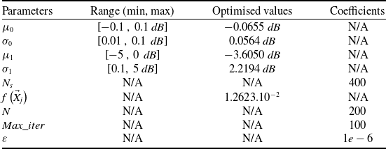
Table 3 reports the results obtained by the learning process based on the GWO algorithm, together with the corresponding three-dimensional fitness landscapes (see Figs 2 and 3). The statistical parameters of the gain
 ${\boldsymbol{\Delta }}{\boldsymbol{G}_k}$
were estimated as
 ${\mu _0}$
 $ = {{\;}} - 0.0655{{\;}}dB$
,
 ${\sigma _0}$
 $ = {{\;}}0.0564{{\;}}dB$
for the normal state, and
 ${\mu _1}$
=
 $ - 3.6050{{\;}}dB$
,
 ${\sigma _1}$
 $ = $
 $2.2194{{\;}}dB$
for the faulty state, with a minimum fitness value of
 $f({{{\vec X}_j}}) = 8.1910 \times {10^{ - 2}}$
.
Optimisation of LNA fault detection parameters using GWO

Table 3 Long description
The table presents the optimization of LNA fault detection parameters using GWO. It has 10 rows and 4 columns. The columns are labeled Parameters, Range (min, max), Optimised values, and Coefficients. The rows list the parameters with their respective ranges, optimized values, and coefficients. Row 1: μ0, [-0.1, 0.1 dB], -0.0655 dB, N/A. Row 2: σ0, [0.01, 0.1 dB], 0.0564 dB, N/A. Row 3: μ1, [-5, 0 dB], -3.6050 dB, N/A. Row 4: σ1, [0.1, 5 dB], 2.2194 dB, N/A. Row 5: Ns, N/A, N/A, 400. Row 6: f(X⃗j), N/A, 1.2623.10^-2, N/A. Row 7: N, N/A, N/A, 200. Row 8: Max_iter, N/A, N/A, 100. Row 9: ε, N/A, N/A, 1e-6.
Fitness function surface over (
 ${\mu _0}$
,
 ${\sigma _0}$
) for the normal operating state.

Fitness function surface over (
 ${\mu _1}$
,
 ${\sigma _1}$
) for the faulty operating state.

Figure 3 Long description
A 3D surface plot represents the fitness function over the variables mu1 and sigma1. The x-axis is labeled mu1 in decibels, ranging from approximately -4.5 to 3. The y-axis is labeled sigma1 in decibels, ranging from approximately 1.8 to 3. The z-axis represents the fitness function f(Xi), ranging from 0.015 to 0.06. The color gradient ranges from blue (lower values) to red (higher values), indicating the magnitude of the fitness function. The surface shows multiple peaks and valleys, suggesting varying levels of fitness across different combinations of mu1 and sigma1. Higher fitness values are indicated by red peaks, while lower values are shown in blue.
The analysis of the convergence surfaces shows that, for the normal state (Fig. 2), the fitness function is smooth and convex, exhibiting a well-defined global minimum. This topology indicates that the normal operating regime is statistically stable and that the algorithm converges easily toward a robust estimation of
 ${\mu _0}$
and
 ${\sigma _0}$
. In contrast, the surface associated with the faulty state (Fig. 3) is more irregular and multimodal, reflecting the increased dispersion of the observations in this regime. Despite this complexity, the global minimum remains identifiable, which justifies the use of a global optimisation strategy to avoid entrapment in local minima. These results confirm that the system exhibits stable behaviour under normal operating conditions and more dispersed behaviour in the faulty regime, and they demonstrate the effectiveness of the proposed approach for the robust estimation of statistical parameters in both states.
2.4 ML models for autotrack prediction
Three ML algorithms were selected to predict the elevation and azimuth parameters of the auto-track system, namely XGBoost, decision trees and KNN. These models were chosen for their ability to model nonlinear relationships, their robustness to noise and their established use in nonlinear regression problems [Reference Chen and Guestrin27–Reference Cover and Hart29].
-
1. XGBoost: A gradient boosting approach based on a set of decision trees optimised to minimise a loss function. It is well known for its robustness against overfitting and its high efficiency when handling large-scale datasets.
-
2. Decision trees: A hierarchical partitioning of the feature space, offering high interpretability while effectively capturing feature interactions and nonlinear patterns.
-
3. KNN: A non-parametric method based on proximity between observations, particularly suitable for modeling complex local structures in the data.
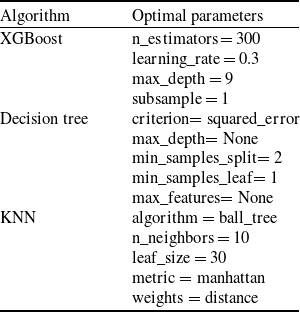
The study is based on a dataset comprising 336,000 measurements collected between 2017 and 2024 from the ALSAT-1B mission, including the actual antenna azimuth and elevation values, the received signal power, as well as the azimuth and elevation measurements provided by the auto-track system. After preprocessing and formatting, the data were used to train the models and to develop an accurate predictor for elevation and azimuth angles. Table 4 summarises the optimised hyperparameters of each algorithm, ensuring an appropriate trade-off between prediction accuracy and generalisation capability.
Tuning of KNN, XGBoost and decision tree algorithms

Table 4 Long description
A table comparing optimal parameters for three algorithms: XGBoost, Decision Tree, and KNN. The table has three rows and two columns. The first column lists the algorithms: XGBoost, Decision Tree, and KNN. The second column lists the optimal parameters for each algorithm. For XGBoost, the optimal parameters are n_estimators = 300, learning_rate = 0.3, max_depth = 9, and subsample = 1. For Decision Tree, the optimal parameters are criterion = squared_error, max_depth = None, min_samples_split = 2, min_samples_leaf = 1, and max_features = None. For KNN, the optimal parameters are algorithm = ball_tree, n_neighbors = 10, leaf_size = 30, metric = manhattan, and weights = distance.
Remark 2. Although all three algorithms are based on standard formulations, the pseudocode is provided only for KNN, which is used as the reference method (baseline) and serves as a point of comparison for the other models. The implementations of XGBoost and decision trees, which are well-documented in the literature [Reference Chen and Guestrin27] and available in established software libraries, are not detailed here.
Algorithm 1: Baseline KNN weighted multi-output regression (optimised with ball tree)
Step 1: Input definition
-
1. Query point:
${x_q}$
: [
${{A}}{{{z}}_{{{mesured}}}}$
,
${{E}}{{{l}}_{{{mesured}}}}$
, Signal Power] -
2. Historical database
$D = \left\{ {\left( {{x_i},{y_i}} \right)} \right\}_{i = 1}^N$
(here
$N = {{\;}}336{{\;}}000{{\;}}measurements$
) -
3. Parameters:
-
•
$v$
= 10 (number of neighbours) -
• Distance metric
$d$
(Manhattan) -
•
$lea{f_{size}} = 30$
-


Step 2: Initialisation phase (baseline setup)
-
1. Build the ball tree spatial index over the dataset
$D$
by recursively partitioning the points into hyperspheres until each leaf node contains at most 30 points.

Step 3: Prediction phase (search for nearest neighbours)
-
1. Go through the ball tree using the triangle inequality to find the nearest neighbours according to the Manhattan distance defined in Equation (15):
(15)
\begin{align}{d_{Manhattan}}({{x_q},{x_i}}) = \mathop \sum \limits_{l = 1}^m \left| {{x_{q,\,f}} - {x_{i,\,f}}} \right|\;\end{align}

where
 $l = 1, \ldots ,{{\;}}m$
indexes the features (azimuth, elevation, signal power).
Step 4: Prediction phase (weight computation and aggregation)
-
1. Compute distance-based weights with numerical stabilisation:
(16)
\begin{align}{{{\omega }}_{{i}}} = \frac{1}{{{{d}}\left( {{{{x}}_{{q}}},\,{{{x}}_{{i}}}} \right) + {{\varepsilon }}}}{{\;}},\,{{\;\;\varepsilon }} \gt 0\;\end{align}
-
• Normalise the weights:
(17)
\begin{align}{{{\omega }}_{{i}}} = \frac{{{{{\omega }}_{{i}}}}}{{\mathop \sum \nolimits_{{{n}} = 1}^{{\nu }} {{{\omega }}_{{n}}}}},\,{{\;}}\mathop \sum \limits_{{{i}} = 1}^{{v}} {{{\omega }}_{{i}}} = 1{{\;}}\end{align}
-
-
2. Compute the multi-output prediction:
(18)
\begin{align}\hat y = \mathop \sum \limits_{i = 1}^\nu {\omega _i}{y_i}\end{align}
-
• Here,
${y_i}$
is the output vector of neighbour
$i$
(azimuth, elevation).
-


Step 5: Output
-
• Return the predicted vector
$\hat y$
, containing azimuth and elevation.

Notes:
 ${x_q} = ({x_{q,1}}$
, …,
 ${x_{q,m}}) \in {R^m}$
, (query point,
 $m = 3$
),
 ${{\;}}{x_i} = ({x_{i,1}}$
, …,
 ${x_{i,m}}) \in {{\mathbb R}^m}$
, (historical input samples),
 ${{\;}}{y_i} = ({y_{i,1}}$
, …,
 ${y_{i,r}}) \in {{\mathbb R}^r}$
, (output vectors,
 $r = 2$
),
 ${{\;\hat y}} = ({\hat y_1}$
, …,
 ${\hat y_{{r}}}) \in {\mathbb{R}^r}$
,
 $d\left( {{x_q},{{\;}}{x_i}} \right) \in {\mathbb{R}^ + },{{\;}}{\omega _i} \in {\mathbb{R}^ + }$
.
3.0 Design and architecture of the proposed auto-tracking system
The experimental work is organised into two main phases. To clearly present our methodology, these two phases are introduced as follows.
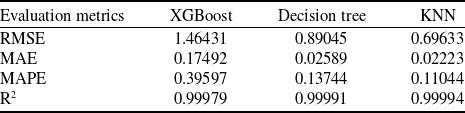
The first phase evaluates XGBoost, decision tree and KNN on eight years’ worth of ALSAT-1B data sampled at one-second intervals. The validation data, corresponding to 20% of the test set, are presented in Table 5. Two representative years, 2017 and 2024, were selected to compare the performance of the models.
Tuning of KNN, XGBoost and decision tree algorithms

Table 5 Long description
A table comparing the performance of XGBoost, decision tree, and KNN algorithms using evaluation metrics. The table has four rows and four columns. The columns are labeled Evaluation metrics, XGBoost, Decision tree, and KNN. The rows are labeled RMSE, MAE, MAPE, and R2. Row 1: RMSE, XGBoost 1.46431, Decision tree 0.89045, KNN 0.69633. Row 2: MAE, XGBoost 0.17492, Decision tree 0.02589, KNN 0.02223. Row 3: MAPE, XGBoost 0.39597, Decision tree 0.13744, KNN 0.11044. Row 4: R2, XGBoost 0.99979, Decision tree 0.99991, KNN 0.99994.
Test configuration at the Oran GS.

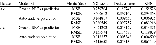
Remark 4. Only the data from 2017 are shown in the figures, as the performance observed in 2024 is similar. The root mean square error (RMSE) values for this latter year are compiled in Table 7 to enable a clear comparison without relying on multiple graphs.
The second phase involves applying the optimal KNN-based solution to ALSAT-1B satellite passes in the presence of a critical fault in the auto-track system. During this phase, the algorithm was tested on real passes from 2025, which constitute unseen data and were not part of the model training dataset (2017–2024). The satellite operates in an SSO with an inclination of 97.78° and a semi-major axis of approximately 7,090 km. The experimental setup (see Fig. 4) relies on the S/X-band GS in Oran, operating in the TM frequency range of 2,200–2,290 MHz and the TC frequency range of 2,025–2,110 MHz. The telemetry data rate reaches 38.4 kbps in S-band and up to 80 Mbps in X-band, with a carrier frequency between 8.025 and 8.400 GHz and an intermediate frequency centred at 720 MHz [Reference Bekkar Djelloul, Djelloul, Bensikaddour and Kaddouri30]. In this second phase, two experimental scenarios were investigated, and their details are presented in the following subsections.
3.1 Results of phase 1: dataset-based algorithms evaluation
Each algorithm was analysed by graphically representing the azimuth and elevation data from the satellite pass in 2017 (AOS: 10:11:39, LOS: 10:16:22). Figures 5 and 6, respectively, show the response of the XGBoost algorithm compared to the reference azimuth and elevation and that of the automatic tracking system upon activation.
Azimuth auto-tracking predicted with XGBoost.

Figure 5 Long description
A line graph showing azimuth auto-tracking predictions using XGBoost compared to ground reference and ground solution data. The horizontal axis represents time in Coordinated Universal Time (UTC) ranging from 10:11:45 to 10:16:15. The vertical axis represents the angle in degrees ranging from 198 to 208 degrees. The graph includes three lines: a green line for ground reference, a red line for auto-track ground solution, and a blue line for XGBoost prediction. The lines show a general downward trend in the angle over time. An inset zooms in on a specific time range from 10:11:40 to 10:11:45, highlighting detailed variations in the angle measurements.
Elevation auto-tracking predicted with XGBoost.

First, it should be noted that at the beginning of the pass, azimuth tracking remained generally acceptable until time 10:45:00, with only slight fluctuations, as shown in the enlarged area of Fig. 5 (auto-track vs REF:
 $MSE{{\;}} = {{\;}}0.003290^\circ $
; XGBoost vs auto-track:
 $MSE{{\;}} = {{\;}}0.114913^\circ $
). After this time, a marked discrepancy appeared and persisted until the end of the pass, indicating a significant degradation in azimuth tracking accuracy.
Regarding elevation (Fig. 6), tracking remains generally stable, with only minor fluctuations. However, a slight degradation is observed between 10:15:40 and 10:16:01 (XGBoost vs. auto-track:
 $MSE{{\;}} = {{\;}}0.035245^\circ $
), indicating significantly better performance compared to azimuth. This degradation, particularly pronounced in azimuth, is primarily attributable to a decrease in signal quality, which can lead to telemetry losses and impair the operation of the automatic tracking system.
For Figs 7 and 8, illustrating the azimuth and elevation estimates obtained with the decision tree algorithm, we initially observe more accurate tracking than that provided by the XGBoost algorithm. At the beginning of the pass, the azimuth calculated by the decision tree closely follows the ground reference trajectory as well as that measured by the auto-track system. However, slight oscillations appear at times 10:12:16, 10:13:12, 10:13:15 and 10:13:26, with respective angles of 204.2°, 201.6°, 202.0° and 201.8° showing deviations from nominal.
Azimuth auto-tracking predicted with decision tree.

Elevation auto-tracking predicted with decision tree.

Figure 8 Long description
Panel: A line graph with the horizontal axis labeled Time in U T C and the vertical axis labeled Angle in degrees. The graph shows three lines representing Ground Reference, Auto-track Ground Solution, and Auto-track Decision Tree Prediction. The Ground Reference line is green, the Auto-track Ground Solution line is red, and the Auto-track Decision Tree Prediction line is blue. The graph includes two zoomed-in insets highlighting specific time intervals. The main trend shows a general decrease in angle over time for all three lines, with the blue line deviating more significantly from the green and red lines as time progresses.
Thereafter, the algorithm very accurately follows the auto-track system, particularly between 10:15:30 and 10:16:22, with a remarkably low RMS error (
 $RMS{{\;}} = {{\;}}0.000136^\circ $
). For elevation, accuracy remains high throughout the pass, as illustrated by the zoom between 10:15:28 and 10:16:01. The RMS error calculated over this period (10:15:28–10:16:22) is
 $0.000772^\circ $
, confirming stability and performance consistency of the algorithm for elevation tracking.
The final algorithm considered for this phase is KNN. Figure 9 shows that the azimuth estimated by KNN very accurately follows the auto-track system throughout the pass. The RMS error calculated over the entire pass is
 $0.000190^\circ $
, confirming high azimuth tracking accuracy.
Azimuth auto-tracking predicted with KNN.

In terms of elevation (Fig. 10), the tracking performance also remains high. Although a brief peak of
 $1.73^\circ $
is observed at 10:16:08, the RMS error over the entire pass remains low, with a value of
 $0.026375^\circ $
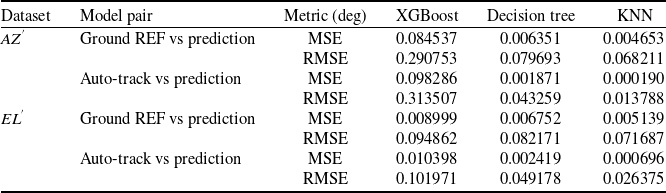
. Overall, the KNN-based algorithm demonstrates high and stable accuracy. Compared to the decision tree, which remains competitive, the KNN offers better overall performance thanks to its ability to adapt to local signal variations, ensuring more accurate tracking in both azimuth and elevation. These observations are consistent with the results presented in Table 6.
Elevation auto-tracking predicted with KNN.

At the end of this section, Table 7 provides a summary of the performance indicators (azimuth and elevation) for all models, in accordance with Remark 4, without multiplying the graphs.
3.2 Results of phase 2: KNN implementation on real satellite passes
Based on the performance observed in Phase 1, KNN was chosen as the implementation algorithm, with the likelihood function used to trigger a switch in the event of an LNA failure in the auto-track chain.
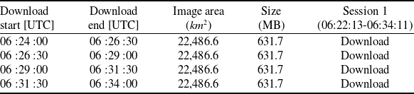
The satellite pass of October 10, 2025 (AOS: 06:22:13, LOS: 06:34:11) was selected as a case study, corresponding to a cumulative volume of downloaded multispectral images of 2,526.8 MB. Table 8 summarises the details related to the image acquisitions.
Remark 5. The likelihood function is applied to elevations above 5°, i.e. when the receiver signal level (RSL) is representative, ensuring reliable process control.
Figure 11 highlights a clear transition from a stationary nominal regime (
 ${H_0}$
) to an unstable degraded regime (
 ${H_1}$
) around 06:27:26, characterised by a significant drop and an increase in its variance associated with an increase in the reflection coefficient
 $\left| {{\Gamma }} \right|$
of the LNA (
 $\left| {{\Gamma }} \right|{{{\;}}_{{{mean\;}}}} \approx 0.35$
).
As shown in Fig. 12, this transition is detected when the log-likelihood ratio abruptly changes from a stable value of approximately −4.3 under normal operating conditions to positive values greater than 10 after 06:27:26, reflecting a statistically significant change in
 $\Delta G$
that renders the observations inconsistent with the nominal model and triggers the fault decision. This separation is quantitatively confirmed by the estimated parameters of the distributions, with
 ${\mu _0} \approx - 0.0655{{\;dB}},\,{\sigma _0} \approx - 0.0564{{\;dB}},$
 ${\mu _1} \approx - 3.6050{{\;dB}},\,{\sigma _1} \approx 2.2194{{\;dB}}$
.
Figures 13 and 14 show the temporal evolution of the satellite’s azimuth (
 $AZ{{'}}$
) and elevation (
 $EL{{'}}$
), comparing the measured values with the predictions provided by the ML-TSR algorithm (see Table 9). Until 06:27:25, the LNA operates in nominal mode (
 ${{\boldsymbol{H}}_0}$
), and the predictions remain consistent with the measurements. At 06:27:26, the likelihood function detects a fault in the LNA, signaling the transition to degraded mode (
 ${{\boldsymbol{H}}_1}$
). From this point onward, the ML-TSR algorithm takes over and initially provides
 $AZ{{'\;}} \approx {{\;}}49.5^\circ $
and
 $EL{{'\;}} \approx {{\;}}32.8^\circ ,$
then values that evolve according to the orbital dynamics until the end of the pass, thus ensuring continuous tracking.
Performance metrics –
 $A{Z^{{'}}}$
&
 $E{L^{{'}}}$
(comparison of models, 21 April 2017, AOS: 10 :11 :39, LOS: 10 :16 :22)

Table 6 Long description
A table comparing performance metrics of different models across two datasets, AZ and EL. The table has 4 rows and 6 columns. Column headers are Dataset, Model pair, Metric (deg), XGBoost, Decision tree, and KNN. Row labels include Ground REF vs prediction and Auto-track vs prediction for each dataset. The table lists values for Mean Squared Error (MSE) and Root Mean Squared Error (RMSE) for each model pair and dataset. For dataset AZ, Ground REF vs prediction shows MSE values of 0.084537 for XGBoost, 0.006351 for Decision tree, and 0.004653 for KNN. RMSE values are 0.290753 for XGBoost, 0.079693 for Decision tree, and 0.068211 for KNN. Auto-track vs prediction shows MSE values of 0.098286 for XGBoost, 0.001871 for Decision tree, and 0.000190 for KNN. RMSE values are 0.313507 for XGBoost, 0.043259 for Decision tree, and 0.013788 for KNN. For dataset EL, Ground REF vs prediction shows MSE values of 0.008999 for XGBoost, 0.006752 for Decision tree, and 0.005139 for KNN. RMSE values are 0.094862 for XGBoost, 0.082171 for Decision tree, and 0.071687 for KNN. Auto-track vs prediction shows MSE values of 0.010398 for XGBoost, 0.002419 for Decision tree, and 0.000696 for KNN. RMSE values are 0.101971 for XGBoost, 0.049178 for Decision tree, and 0.026375 for KNN.
Performance metrics –
 $A{Z^{{'}}}$
&
 $E{L^{{'}}}$
(comparison of models, 19 Nov 2024, AOS: 19 :32 :03, LOS: 19 :40 :50)

Table 7 Long description
A table comparing performance metrics of different models. The table has 2 groups of rows labeled AZ and EL, 3 columns labeled Model pair, Metric (deg), and XGBoost, Decision tree, KNN. Row 1: Model pair, Ground REF vs prediction; Metric (deg), MSE; XGBoost, 0.259704; Decision tree, 0.157743; KNN, 0.155526. Row 2: Model pair, Auto-track vs prediction; Metric (deg), MSE; XGBoost, 0.144817; Decision tree, 0.009556; KNN, 0.006925. Row 3: Model pair, Ground REF vs prediction; Metric (deg), RMSE; XGBoost, 0.509612; Decision tree, 0.397169; KNN, 0.394368. Row 4: Model pair, Auto-track vs prediction; Metric (deg), RMSE; XGBoost, 0.380549; Decision tree, 0.097757; KNN, 0.083216. Row 5: Model pair, Ground REF vs prediction; Metric (deg), MSE; XGBoost, 0.024203; Decision tree, 0.013129; KNN, 0.014371. Row 6: Model pair, Auto-track vs prediction; Metric (deg), MSE; XGBoost, 0.013377; Decision tree, 0.005348; KNN, 0.004509. Row 7: Model pair, Ground REF vs prediction; Metric (deg), RMSE; XGBoost, 0.155574; Decision tree, 0.114583; KNN, 0.119879. Row 8: Model pair, Auto-track vs prediction; Metric (deg), RMSE; XGBoost, 0.115658; Decision tree, 0.073130; KNN, 0.067149.
Scheduled ALSAT-1B image acquisitions and related operations

Table 8 Long description
The table has five rows and five columns. The columns are labeled Download start (UTC), Download end (UTC), Image area (km^2), Size (MB), and Session 1 (06:22:13-06:34:11). The rows provide details for each image acquisition. Row 1: Download start, 06:24:00; Download end, 06:26:30; Image area, 22,486.6; Size, 631.7; Session 1, Download. Row 2: Download start, 06:26:30; Download end, 06:29:00; Image area, 22,486.6; Size, 631.7; Session 1, Download. Row 3: Download start, 06:29:00; Download end, 06:31:30; Image area, 22,486.6; Size, 631.7; Session 1, Download. Row 4: Download start, 06:31:30; Download end, 06:34:00; Image area, 22,486.6; Size, 631.7; Session 1, Download.
Transition from nominal to degraded LNA regime (
 ${H_0}$
→
 ${H_1}$
): output ΔG dynamics.

Statistical detection of LNA defects.

ML-TSR azimuth auto-tracking predictions profile during phase 2.

ML-TSR elevation auto-tracking predictions profile during phase 2.

Although a fault in the LNA was observed for approximately 4 s around 06:27:26, it did not cause an interruption of the transmission, as illustrated in Fig. 15. This event resulted in a transient degradation of the RSL, which briefly dropped to approximately
 $ - 58{{\;}}dBm$
, accompanied by an increase in the LNA’s reflection coefficient, momentarily rendering the observations incompatible with the nominal regime. The likelihood function decision triggered the activation of the ML-TSR controller, which took over the auto-tracking chain and allowed the tracking to stabilise again from 06:27:30. The RSL then recovered to values approximately between
 $ - 55$
and
 $ - 42{{\;}}dBm$
, with the link lock maintained, ensuring continuity of the transmission until the Loss of Signal (LOS).
Table 9 illustrates the values distinguishing the nominal state of the LNA from the period affected by a fault. In the absence of a fault, the average
 $\Delta G{{\;}}\left( {dB} \right)$
corresponds to the component specifications and remains within the normal operating range. In the presence of a fault, according to assumption 1, the average ΔG is in the range
 $\left[ { - 1.92,{{\;}} - 0.28{{\;}}dB} \right]$
, indicating a potential out-of-specification risk requiring careful monitoring.
4.0 Conclusion
The combination of the KNN algorithm with GWO for tuning the statistical parameters of the likelihood function enabled the development of a robust and fault-tolerant tracking system, particularly resilient to LNA failures. The method was first validated on 20% of an eight-year dataset (2017–2024), including the operational parameters of the ALSAT-1B GS, and subsequently evaluated on an independent satellite pass in 2025 under real fault conditions.
During the LNA degradation event (Avg. ΔG = −0.5483 dB), the likelihood-based decision mechanism triggered a switch to the ML-assisted tracking mode within 4 s, restoring the received signal level to its nominal operating range (−55 to −42 dBm). This rapid adaptation ensured uninterrupted mission continuity and enabled the successful download of four images totaling 2,526.8 MB, with no data loss observed.
These results demonstrate the effectiveness of the proposed hybrid approach for real-time fault detection and mitigation in satellite GS operations. Beyond the specific ALSAT-1B case study, the framework can be extended to other RF subsystems and fault scenarios, providing a general methodology for improving the reliability and autonomy of future ground segment infrastructures.
Scheduled ALSAT-1B image acquisitions and related operations

Table 9 Long description
A table comparing performance metrics of different models for azimuth and elevation predictions. The table has four rows and three columns. Column headers are Model pair, Metric (deg), and values under XGBoost, Decision tree, and KNN. Row labels are AZ' Ground REF vs prediction MSE, AZ' Ground REF vs prediction RMSE, AZ' Auto-track vs prediction MSE, AZ' Auto-track vs prediction RMSE, EL' Ground REF vs prediction MSE, EL' Ground REF vs prediction RMSE, EL' Auto-track vs prediction MSE, and EL' Auto-track vs prediction RMSE. Row 1: XGBoost, 0.084537, 0.006351, 0.004653. Row 2: XGBoost, 0.290753, 0.079693, 0.068211. Row 3: XGBoost, 0.098286, 0.001871, 0.000190. Row 4: XGBoost, 0.313507, 0.043259, 0.013788. Row 5: XGBoost, 0.008999, 0.006752, 0.005139. Row 6: XGBoost, 0.094862, 0.082171, 0.071687. Row 7: XGBoost, 0.010398, 0.002419, 0.000696. Row 8: XGBoost, 0.101971, 0.049178, 0.026375.
RSL profile during phase 2.



 μ0
 σ0

 μ1
 σ1


 AZ′
 EL′
 AZ′
 EL′

 H0
 H1






