





Non-technical Summary
San Salvador Island in the Bahamas is covered by many saltwater lakes that formed thousands of years ago when rising sea levels flooded the island’s lowlands, making these lakes unique opportunities to study evolution in small, isolated communities of marine organisms. We found these lakes to be home to thriving populations of a small clam called Ctena, which live buried in lake sediments and rely on bacteria inside their bodies for nutrition (a feeding strategy called chemosymbiosis). By comparing both living Ctena and preserved dead shells from the sediment, we found strong differences in shell size and shape among lakes, and more modest differences between living and dead within each lake. These morphological differences appear to reflect adaptations of their chemosymbiotic lifestyle to each lake’s distinct environmental conditions. Ongoing genetic analyses suggest these Ctena are all one species, meaning differences we observe are likely caused by environmental conditions in each lake rather than the formation of new species. Our results show how environmental variation can shape the form of organisms over relatively short evolutionary timescales, and how preserved shells can help bring temporal context to these patterns.
Introduction
Lakes can serve as natural experiments of adaptive radiation, especially those that (1) have ecologically distinct habitats, (2) persist on evolutionary timescales, and (3) harbor nonrandom subsets of the regional fauna (Schön and Martens Reference Schön and Martens2004). Classic examples include repeated colonization of post-glacial lakes by ancestrally marine and anadromous three-spine sticklebacks (Reid et al. Reference Reid, Bell and Veeramah2021; Aguirre et al. Reference Aguirre, Reid, Rivera, Heins, Veeramah and Bell2022); the radiation of more than 350 species of endemic amphipods in Lake Baikal—Earth’s oldest and deepest freshwater body—over multiple colonization events (Macdonald et al. Reference Macdonald, Yampolsky and Duffy2005; Ironside and Wilkinson Reference Ironside and Wilkinson2018); and perhaps most profoundly, the explosive diversification of more than 1200 species of cichlids in the African Great Lakes over the last 100,000 to 1.2 million years (Meier et al. Reference Meier, Marques, Mwaiko, Wagner, Excoffier and Seehausen2017; Santos et al. Reference Santos, Lopes and Kratochwil2023). Although large and ancient lakes have offered numerous insights into the nature of adaptive radiation, it is equally important to examine recently formed Holocene habitats, where early processes in adaptive divergence may be more readily observed and mechanistically understood.
San Salvador Island in the Bahamas has numerous anchialine lakes that formed within karstified, interdunal depressions during the Holocene transgression over the last 10,000 years (Teeter Reference Teeter, Curran and White1995; Park Boush et al. Reference Park Boush, Myrbo and Michelson2014). These lakes range from brackish to hypersaline and experience delayed tidal fluctuations due to variable hydrologic connectivity to the ocean through networks of submerged karst conduits (Davis and Johnson Reference Davis, Johnson and Mylroie1989; Godfrey et al. Reference Godfrey, Edwards, Smith and Davis1994; Hagey and Mylroie Reference Hagey, Mylroie, Curran and White1995; Smith et al. Reference Smith, Wynn, Scharping, Moore, Garey and Onac2020). The distinct habitats of San Salvador’s anchialine lakes led Edwards (Reference Edwards, Elliot, Edwards and Godfrey1996) to postulate that inhabitants could provide evidence of adaptive radiation since the start of the Holocene, whereby morphological and genetic differentiation would occur over a relatively rapid time frame. Indeed, two endemic species of Cyprinodon pupfishes from the San Salvador lakes are distinct from widely distributed western Atlantic taxa and distinguished by jaw morphologies that enable specialized feeding strategies, including durophagy of shellfish (Turner et al. Reference Turner, Duvernell, Bunt and Barton2008; Martin and Wainwright Reference Martin and Wainwright2013; Chan et al. Reference Chan, Colaco, Martin and Evans2024). It is therefore worth investigating whether similar patterns of ongoing adaptive change are evident from other members of these anchialine lake communities. Further, benthic mollusks are a particularly compelling taxonomic candidate, as they may be trophically linked to durophagous pupfish in these lakes.
Here, we tested for morphological divergence of phenotypic traits in lake-dwelling lucinid bivalves that we assign to the genus Ctena (previously misidentified as Codakia orbicularis; Edwards Reference Edwards, Clark-Simpson and Smith2001; Lanterman et al. Reference Lanterman, Button, Erdman, Rathcke and Hayes2007). We discovered dense populations of Ctena sp. inhabiting carbonate-rich clays within karst pockets along the shorelines of small anchialine lakes in northern San Salvador, representing a novel habitat occurrence for lucinids. These lake-dwelling Ctena resemble C. imbricatula that occur in adjacent coastal waters (Taylor and Glover Reference Taylor and Glover2016), but ongoing genomic analyses indicate that these lake-dwelling populations encompass a single species without a clear phylogenetic relationship to other Ctena spp. from the Caribbean and Atlantic basins (Long-Fox et al. Reference Long-Fox, Anderosn, Lim, Campbell, Kokesh, Paterson and Engel2025). However, morphometric analyses may help in supporting genomic work in identifying and describing species, especially when evaluating both extant and extinct taxa (Lee and Palci Reference Lee and Palci2015; Aguirre et al. Reference Aguirre, Richiano, Álvarez and Farinati2016; Holvast et al. Reference Holvast, Celik, Phillips and Wilson2024). To quantify both spatial and temporal dimensions of morphological divergence, our approach employs two-dimensional geometric morphometrics of internal shell features on both live- and dead-collected shells from three of San Salvador’s anchialine lakes.
Intraspecific morphological variation of these anatomical features could be, at least initially, a plastic response to environmental conditions that vary geographically, which in turn could drive ecological separation (e.g., Li et al. Reference Li, Li, Song, Meng, Guo, Li and Li2018; Richards et al. Reference Richards, Cruz, Shapiro, Wootton and Pfister2025). As such, we evaluated lake sediment descriptions and pore-water geochemistry to identify environmental conditions that were likely to be important to the lifestyle of Ctena and that could explain spatial patterns in morphological variation observed among populations. Further, the time-averaged nature of dead-shell debris in surficial sediments has made live–dead comparisons an increasingly common tool for detecting temporal changes in ecological or environmental conditions over the window of time averaging, typically spanning centuries to millennia in coastal seabeds (Kidwell and Tomašových Reference Kidwell and Tomašových2013). The inclusion of dead-collected shells in this study was thus motivated to test temporal changes in Ctena morphology within and among lake populations.
Lucinid bivalves, like Ctena, are an especially interesting study system because of their chemosymbiotic lifestyle, wherein they harbor bacterial endosymbionts that oxidize reduced sulfur compounds and provide a critical ecosystem service for the health of seagrass beds, mangrove swamps, and other coastal habitats (van der Heide et al. Reference van der Heide, Govers, DeFouw, Olff, van der Geest, van Katwijk and Piersma2012; Lim et al. Reference Lim, Alexander, Engel, Paterson, Anderson and Campbell2019; Giani et al. Reference Giani, Lim, Anderson, Paterson, Engel and Campbell2025). Lucinids obtain endosymbionts via horizontal transmission from the surrounding environment throughout their life, rather than vertically from parent to offspring (Gros et al. Reference Gros, Elisabeth, Gustave, Caro and Dubilier2012; Elisabeth et al. Reference Elisabeth, Gustave and Gros2012), and possess several key anatomical features associated with their infaunal chemosymbiotic lifestyle. Diagnostic on the interiors of both live- and dead-collected shells is an anterior adductor muscle scar detached from the pallial line to create an inhalant channel, which is thought to facilitate respiration and circulate oxygenated blood via a pallial blood vessel to other mantle tissues (Allen Reference Allen1958; Stanley Reference Stanley1970; Taylor and Glover Reference Taylor, Glover, Harper, Taylor and Crame2000; Anderson Reference Anderson, Hembree, Platt and Smith2014). Although all known lucinid species to date form chemosymbiotic associations with thiotrophic bacteria, it is unclear whether this process is obligatory (as it is known for the Solemyidae) or facultative (as is known for the Thyasiridae; Taylor and Glover Reference Taylor, Glover and Kiel2010). However, Duplessis et al. (Reference Duplessis, Dufour, Blankenship, Felbeck and Yayanos2004) suggest that some anatomical features of lucinids are consistent with the ability to perform particulate feeding.
Materials and Methods
Sample Collection
Ctena specimens were collected from three small anchialine lakes surveyed from 2016 through 2018, where previous surveys report the presence of Ctena (as Codakia; Edwards Reference Edwards, Clark-Simpson and Smith2001). The lakes are about 1 km south of the Gerace Research Centre (GRC) adjacent to the northern coast of San Salvador Island, the Bahamas (Fig. 1), with shorelines separated by a minimum of ~50 m. This proximity ensures that lakes experienced the same climatic variation and hurricane recurrence, which has varied across the island and from the rest of the Caribbean region (Park Reference Park2012). Four stations of 50 × 50 cm quadrats were established in each lake. When possible, stations were excavated using a shovel or hand trowel to a depth of at least 30 cm, although limestone bedrock was encountered at 10–15 cm depth at several stations due to the irregular karst surface. Excavated sediments were sieved through 3 mm mesh to isolate bivalves. While this mesh size almost certainly caused us to miss juveniles and the smallest-bodied individuals (Kidwell Reference Kidwell2013), it was suitable for collecting longer-lived adults and capturing the upper limits of population body sizes. Accounting for permitted per-quadrat sampling limits, we collected 44 out of 47 encountered living Ctena specimens at Crescent Pond, 86 out of 173 at Moon Rock Pond, and 85 out of 85 at Pain Pond. For dead specimens (n = 562 for Crescent Pond, 231 for Moon Rock Pond, and 332 for Pain Pond), we collected only articulated shells under the assumption these specimens died in situ or experienced minimal postmortem transport. Cleaned shells (stored dry) and soft tissues (initially preserved in RNAlater and later stored in ethanol at −20°C) are accessioned and cataloged at the Museum of Geology at the South Dakota School of Mines and Technology (SDSM). SDSM catalog numbers for live-collected specimens are indicated as specimen names in the online dataset (see “Data Availability Statement”). Dead-collected specimens were randomly selected from death assemblage samples for Crescent Pond (catalog nos. SDSM 115684, 138088, 140321, 140344, 140349), Moon Rock Pond (115745, 138089, 140356, 140381, 140406), and Pain Pond (140453, 140454, 140477, 140500, 140539).
Map of San Salvador Island, the Bahamas, with filled circles marking marine sites used for geochemical comparisons to lake conditions and the open square indicating inset region containing lakes studied here (photographs). Dotted line in inset map represents marked trails near the Gerace Research Centre (GRC). Stars at Crescent Pond, Moon Rock Pond, and Pain Pond indicate approximate sampling area along each lakeshore. Small circles indicate locations of karst conduit openings. Inset map after Knowlton et al. (Reference Knowlton, Barr, Marshalonis, Spark and Gross2014).

Figure 1. Long description
The image consists of three main sections.
On the left is a geographical map of San Salvador Island with a 5 kilometer scale bar. Two filled circles mark marine sites: Graham’s Harbour (North Ocean Control) at the northern tip and Pigeon Creek (South Ocean Control) at the southern tip. An open square in the Northeast indicates the study area.
In the center is a detailed inset map of the study area with a 500 meter scale bar. At the top is the Gerace Research Centre (G RC). Dotted lines represent trails connecting several ponds. Reckley Hill Pond is in the Northeast. Crescent Pond is centrally located with two small circles indicating karst conduit openings on its West side and a star marking the sampling area on its East side. To the South and Southeast are Pain Pond and Moon Rock Pond, both marked with stars for sampling areas and small circles for karst conduits. Wild Dilly Pond, Oyster Pond, and Osprey Pond are located to the Southwest.
On the right is a vertical column of three photographs showing the lakeshores of Crescent Pond, Moon Rock Pond, and Pain Pond. Each photo depicts calm water surrounded by low-lying green vegetation under a blue or slightly overcast sky.
Pore-water geochemical data were collected in the field at sediment depths of 10–20 cm using a hollow stainless-steel piezometer fit with peristaltic pump tubing connected to a syringe to create a low-flow pump. Pore-water temperature, pH, and conductivity, as well as dissolved oxygen, dissolved sulfide, and alkalinity concentrations were quantified, following methods described by Green-García and Engel (Reference Green-Garcia and Engel2012). The pore-water and overlying lake geochemistry dataset included samples from Crescent Pond (n = 4), Moon Rock Pond (n = 4), and Pain Pond (n = 1), with the low number of sample sites reflecting the challenge in obtaining pore-water-only samples when depth to bedrock is shallow. We also collected pore-water samples at Pigeon Creek (n = 9) on the southeast corner of San Salvador and Graham’s Harbour (n = 4) north of the GRC to compare pore-water conditions found in open-marine settings with those measured from anchialine lakes (Fig. 1). After log-transforming and z-score scaling all pore-water variables, we evaluated overall variation patterns among lakes and ocean controls using redundancy analysis (RDA).
Shell Data Preparation
Images of shell interiors from left valves were obtained using a flatbed scanner at a resolution of 2400 dpi. We digitized landmarks using tpsDIG2 (Rohlf Reference Rohlf2008). During digitization, specimens were removed if image quality or physical condition obscured features necessary for landmarking. In the final dataset, 40, 57, and 43 live-collected specimens were retained from Crescent Pond, Moon Rock Pond, and Pain Pond, respectively. To make live and dead sample sizes similar, 50 dead-collected specimens from each lake were randomly subsampled and added to the dataset. Replicating statistical analyses (see next section) using a second set of 50 randomly selected dead specimens generated similar results, suggesting that 50 dead-collected specimens from each lake adequately captured shape and size variation within the death assemblage.
We replicated the landmark configuration defined by Anderson (Reference Anderson, Hembree, Platt and Smith2014), which focused on capturing the inhalant channel (Fig. 2). Landmarks 4 and 5 are defined as Type I landmarks, representing the junctions between each adductor muscle scar and the pallial line (Bookstein Reference Bookstein1991). Landmarks 1, 2, 3, and 6 are defined as Type II landmarks, representing localized maxima in curvature for the shell beak, dorsal and ventral ends of the anterior adductor scar, and the dorsal end of the posterior adductor scar, respectively. In addition, three semilandmark curves were added to the configuration to capture additional shell shape variation (Fig. 2). The first curve, with five semilandmarks, connects fixed landmarks 3 and 4, following the ventral side of the anterior adductor scar. The second curve, containing 10 semilandmarks, traces the pallial line between fixed landmarks 4 and 5. The third curve, containing 20 semilandmarks, follows the outline of the shell and is anchored by landmark 1 at the beak. Semilandmarks were resampled by length in tpsDIG2 to reposition them at equidistant points along their respective curves.
Photographed interior of a dead-collected Ctena shell with well-preserved features. Left, biologically significant features preserved on the interiors of dead shells, including the anterior adductor scar (aa), inhalant channel (ic), posterior adductor scar (pa), pallial blood vessel (pb), and pallial line (pl). Right, landmark configuration used in this study, as described in the “Materials and Methods.” Anterior direction to the right. Scale bar, 1 cm.

All succeeding preparations and analyses were performed in version 4.5.0 of the R programming environment (R Core Development Team 2025), with specialized functions for morphometrics supplied by the packages geomorph (Baken et al. Reference Baken, Collyer, Kaliontzopoulou and Adams2021; Adams et al. Reference Adams, Collyer, Kaliontzopoulou and Baken2025) and Morpho (Schlager Reference Schlager, Zheng, Li and Szekely2017). Landmark data were parsed into three datasets: live-collected shells only, dead-collected shells only, and combined live- and dead-collected shells. Raw landmark positions for each dataset were superimposed using a generalized Procrustes analysis (GPA; Rohlf and Slice Reference Rohlf and Slice1990) to correct for scaling, translational, and rotational differences among digitized specimens with the gpa function in geomorph. GPA also calculates the centroid size of each specimen, defined as the square root of the sum of squared distances between all landmarks and the configuration’s centroid. Following GPA, specimens were investigated for potential outliers, defined as those with a Procrustes distance that exceeds the upper quartile of all specimens from the mean shape. Seven outliers were detected, but were retained in the dataset after reinspection that verified the accuracy of landmark placements.
Statistical Analyses
To test for differences in mean shell shape and centroid size, we performed two-sided Procrustes analysis of variance (ANOVA) using the procD.lm function in geomorph and 5000 iterations for significance testing. For the datasets including only live- or only dead-collected specimens, Procrustes ANOVA tested differences in valve shape among lakes (Crescent Pond, Moon Rock Pond, and Pain Pond). For the dataset combining live- and dead-collected specimens, analyses were expanded using a factorial model that included life state (live vs. dead) and its interaction with lakes (e.g., shape or size ~ lake + state + lake:state). We also tested for differences in allometry (i.e., the relationship between shape and size) in the live–dead dataset among lakes and between life states by performing Procrustes ANOVA for shape with centroid size as a covariate. Each test used a residual randomization permutation procedure (RRPP) to increase statistical power and more efficiently calculate descriptive statistics from high-dimensional landmark and semilandmark data (Collyer and Adams Reference Collyer and Adams2018, Reference Collyer and Adams2024). The p-values were generated using 10,000 permutations and considered statistically significant if less than 0.05. We followed Procrustes ANOVA tests with significant results with post hoc pairwise comparisons of group means and allometric slopes using the pairwise function in geomorph and adjusting the resulting p-values with a Holm adjustment procedure.
Shape variation among specimens for each of the three datasets was visualized using principal component analysis (PCA) with the gm.prcomp function in geomorph, with convex hulls drawn around each lake assemblage to visualize groupwise variation. As a complement to PCA, we used canonical variate analysis (CVA) with the CVA function in Morpho. Although PCA ordinates specimens along axes that retain as much of the total morphological variance as possible, CVA specifically generates axes that most effectively discriminate between a priori defined groups among samples (Webster and Sheets Reference Webster, Sheets, Alroy and Hunt2010). We used jackknife reassignment tests to determine the accuracy of recovered group assignments from CVA relative to known group identities. Allometric trends were visualized by plotting each regression’s shape scores from Procrustes ANOVA against log-transformed centroid size (Drake and Klingberg Reference Drake and Klingenberg2008).
A phenotypic trajectory analysis (PTA; Adams and Collyer Reference Adams and Collyer2009) was performed to examine relationships between mean shapes for co-occurring life and death assemblages as shape-change vectors superimposed on model-fit specimen coordinates for each lake. PTA produces pairwise statistical tests for differences in vector magnitude (i.e., the amount of shape change between paired group means) and vector angle (i.e., the difference in the direction of change) among lakes. PTA was visualized by superimposing group means onto a PCA of Procrustes model-fit data.
To visualize overall shape differences among live and dead assemblages from the three lakes, we generated thin-plate spline (TPS) deformation grids, which illustrate the displacement of landmarks and semilandmarks between two configurations on a two-dimensional surface (Bookstein Reference Bookstein1989). Using the plotRefToTarget function in geomorph, we used the global mean landmark configuration for all specimens in the full dataset as the reference to which the groupwise mean landmark configurations were each set as the targets. To aid in visualization of shape changes, TPS deformations were magnified by a factor of four (i.e., artificially exaggerating the amount of shape change). To further support interpretations from TPS grids, we calculated the ratio of inner mantle area (e.g., that inside the pallial line) to the outer margin area (e.g., that of the entire shell) to quantify the proportion of shell area occupied by soft mantle tissues. Ratios were tested for significant differences among lakes and life states using a two-way ANOVA.
Results
Collections and Habitat Characteristics
Open-lake sediment was generally devoid of living Ctena, but we encountered dense populations in sediment that filled irregular karst holes or larger pockets along the shorelines of all three lakes. Sediment in Crescent Pond, sampled in May 2016 and December 2017, was a combination of fine-grained dark carbonate mud overlain by flocculent organics (see also Godfrey et al. Reference Godfrey, Edwards, Smith and Davis1994; Edwards Reference Edwards, Elliot, Edwards and Godfrey1996). Benthic vegetation consisted of macrophytic algae (Batophora and Acetabularia) and dispersed clumps of the seagrass Ruppia maritima. During summertime sampling, Crescent Pond also had abundant populations of Arenicola lugworms and dense concentrations of their egg sacs. Moon Rock Pond sediment, sampled in May 2016 and December 2017, was a fine-grained, white carbonate mud (see also Freile et al. Reference Freile, Faulker, Edge, Davis and Gamble2006) with scattered small patches of algal mats. Pain Pond sediment, sampled in January 2018, was a dark, organic-rich, fine-grained mud mixed with microscopic carbonate shells and sponge spicules composed of silica (Godfrey et al. Reference Godfrey, Edwards, Smith and Davis1994). Live Ctena were constrained to sediment-filled karst pockets along the lake’s edge. Ctena was the only lucinid collected from each lake, but other abundant bivalves encountered alive or dead included Anomalocardia puella and Isognomon alatus in Crescent Pond, Brachidontes exustus and Tampaella mera in Crescent Pond and Moon Rock Pond, and Gemma gemma in Pain Pond.
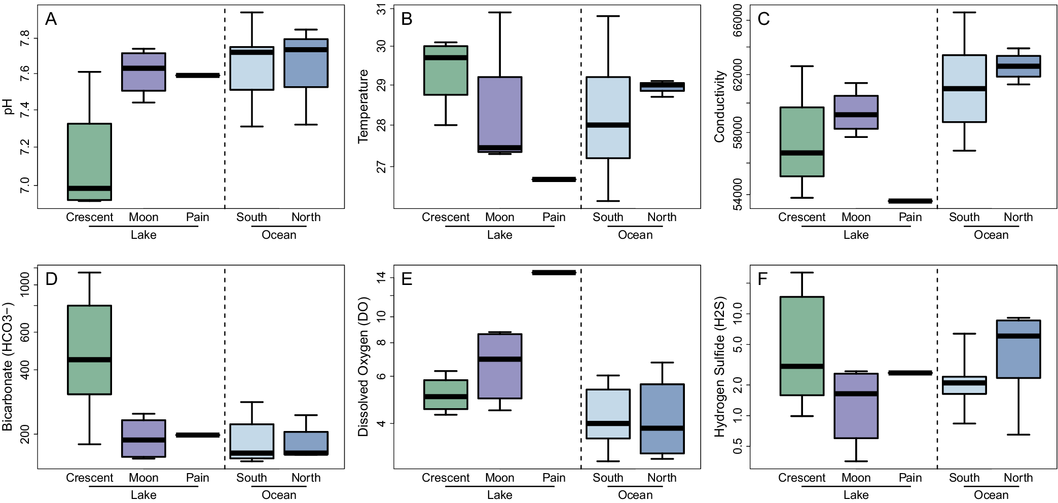
Despite the limited sample sizes, visual examination of pore-water geochemistry measurements indicated several differences among the three lakes and open-marine conditions (Fig. 3). Median and interquartile values for pH were notably low at Crescent Pond compared with other lake and ocean pore-waters (Fig. 3A). Median temperature was also relatively high for Crescent Pond and notably low for Pain Pond (Fig. 3B). Conductivity was generally lower for lakes compared with the open ocean, especially at Pain Pond (Fig. 3C). Alkalinity represented as bicarbonate concentration was notably higher at Crescent Pond (Fig. 3D), and dissolved oxygen values were higher for Moon Rock Pond and especially Pain Pond (Fig. 3E). Finally, median sulfide concentrations were similar for all lakes, though the interquartile range for Crescent Pond was relatively high and that for Moon Rock Pond was relatively low (Fig. 3F). Open-ocean control samples were similar in pore-water geochemical measurements, with the exception to sulfide, which was elevated at Graham’s Harbour on the north side of the island compared with Pigeon Creek in the south. Pore-water RDA further demonstrated a general trend toward lower conductivity for lakes compared with values for ocean controls (Fig. 4).
Measurements for (A) pH, (B) temperature (Celsius), (C) conductivity (μS/cm), (D) alkalinity as bicarbonate concentration (mg/L), (E) dissolved oxygen concentration (mg/L), and (F) dissolved sulfide concentration (mg/L) from pore-water samples from Crescent Pond (n = 4), Moon Rock Pond (n = 4), Pain Pond (n = 1), the south coast ocean control represented by Pigeon Creek (n = 9), and the north coast ocean control at Graham’s Harbour (n = 4).

Figure 3. Long description
A multi-panel figure containing six box plots labeled A through F. Each plot features a vertical dashed line separating three Lake sites (Crescent in green, Moon in purple, Pain in black) from two Ocean sites (South in light blue, North in dark blue).
* Panel A: pH. Lake values range from approximately 6.9 to 7.7. Ocean values are higher, ranging from 7.3 to 7.9.
* Panel B: Temperature in degrees Celsius. Crescent and Moon lakes range from 27.5 to 30.5. Pain Lake is a single point near 26.8. Ocean sites range from 26 to 31.
* Panel C: Conductivity in mu S/cm. Lake values range from 54,000 to 62,000, with Pain Lake significantly lower at approximately 53,500. Ocean values are higher, between 57,000 and 66,000.
* Panel D: Bicarbonate HCO3 in m g/L. Crescent Lake shows high variability from 200 to over 1,000. Other sites are lower, mostly clustered between 100 and 300.
* Panel E: Dissolved Oxygen DO in m g/L. Lake sites range from 4 to 9, while Pain Lake is an outlier at approximately 14. Ocean sites are lower, ranging from 2 to 7.
* Panel F: Hydrogen Sulfide (H2 S) in mg/L on a logarithmic scale. Crescent Lake has the highest range, reaching up to 20. Other sites range from 0.3 to 10.
Biplot of the first two axes from redundancy analysis (RDA) for log-transformed and z-scaled pore-water geochemistry data. Percentage values on axis labels indicate the amount of total variation accounted for by that axis. Convex hulls are drawn around each location to aid in visualizing groupwise variation. Labeled arrows indicate the direction of influence by each geochemical parameter.

Figure 4. Long description
The x-axis is RDA 1, accounting for 42.33 percent of variation, ranging from -0.6 to 0.6. The y-axis is RDA 2, accounting for 25.25 percent of variation, ranging from -0.6 to 0.6. Six geochemical vectors originate from the center. Temperature points North-Northwest. H2 S points Northeast. HCO3 points East. DO points South. pH points West-Southwest. Conductivity points Northwest. Data points are grouped by location. Crescent Pond (green circles) is concentrated in the East and Northeast quadrants. Moon Rock Pond (purple squares) is concentrated in the South and Southwest quadrants. Pain Pond (orange triangle) is a single outlier in the Southeast quadrant. North Grahams Harbour (dark blue diamonds) and South Pigeon Creek (light blue inverted triangles) are heavily overlapped in the Northwest and West quadrants. Each group except Pain Pond is enclosed by a colored convex hull line matching its symbol color.
Combining qualitative sedimentological and quantitative geochemical observations, we characterize each lake as having the following environmental conditions: (1) Crescent Pond is relatively organic-rich, reducing, and weakly buffered; (2) Moon Rock Pond is oligotrophic, carbonate-dominated, and well-buffered; and (3) Pain Pond is diluted of ions, highly oxygenated, and rich in biogenic silica.
Shape and Size Variation
Procrustes ANOVA of Ctena shell shape revealed significant differences among lakes for analyses of both life assemblages (F = 12.49, p < 0.001) and death assemblages (F = 13.06, p < 0.001), as well as the interaction between lake and life state in the full dataset (F = 5.69, p < 0.001; Table 1A). Similarly, Procrustes ANOVA testing for variation in centroid sizes revealed significant differences among lakes for life assemblages (F = 159.81, p < 0.001), death assemblages (F = 76.88, p < 0.001), and the interaction term for the full dataset (F = 8.52, p < 0.001; Table 1B). Further, Procrustes ANOVA revealed that shell shape significantly covaried with size in all three datasets, indicating allometric growth (Table 1C). Finally, the interaction between size and lake was significant for life assemblages (F = 1.97, p = 0.016), but not for death assemblages (F = 0.77, p = 0.727). For the full dataset, the interaction terms between centroid size and lake identity (F = 1.45, p = 0.029) or life state (F = 1.03, p = 0.011) were significant, but the interaction of all three model effects was not significant (F = 0.95, p = 0.499).
Results from Procrustes ANOVA of (A) shell shape variation, (B) centroid size variation, and (C) shape variation with centroid size as a covariate (e.g., a test of allometry), assessed for live-collected specimens, dead-collected specimens, and combined live and dead specimens. Bolded p-values indicate significance (p < 0.05). df = degrees of freedom; F = observed F-value; and p = p-value

Table 1. Long description
The table is divided into three sections: (A) Shape, (B) Size, and (C) Allometry. Each section contains columns for df, F, and p values categorized under Live, Dead, and Live and Dead specimens.
* Section (A) Shape: For the Lake variable, p-values are less than 0.001 across all specimen types. In the Live and Dead category, State and Lake-State interaction also show p-values less than 0.001. Residual d f values are 137 for Live, 147 for Dead, and 284 for Live and Dead.
* Section (B) Size: Lake shows significant p-values (less than 0.001) for all groups. In the Live and Dead category, State is not significant (p equals 0.196), but the Lake-State interaction is significant (p less than 0.001).
* Section (C) Allometry: Size and Lake variables show significant p-values (less than 0.001) across all specimen types. The Size-Lake interaction is significant for Live (p equals 0.016) and Live and Dead (p equals 0.029) but not for Dead (p equals 0.727). In the Live and Dead category, State (p less than 0.001), Size-State (p equals 0.011), and Lake-State (p less than 0.001) are significant, while the three-way Size-Lake-State interaction is not significant (p equals 0.499). Residual d f values are 134 for Live, 144 for Dead, and 278 for Live and Dead.
The first three axes of PCA accounted for ~58% of shape variation for live-only (Fig. 5A,D), 57% for dead-only (Fig. 5B,E), and 54% for the full dataset (Fig. 5C,F). For all datasets assessed, variation along PC 1 and PC 3 did not separate lake assemblages. Moon Rock Pond, however, exhibited detectable separation from those for Crescent Pond and Pain Pond along PC 2, particularly for live specimens.
Plots of the first three axes from principal component analysis (PCA) for shell morphometric data of lake-dwelling Ctena, assessing (A, D) live-collected specimens, (B, E) dead-collected specimens, and (C, F) all specimens combined into a single dataset. Percentage values on axis labels indicate the amount of total morphological variation accounted for by that axis. Convex hulls are used to aid in visualizing groupwise variation.

Figure 5. Long description
A multi-panel scatter plot arrangement with two rows and three columns.
Top Row (P C 1 vs PC 2):
* Panel A (Live): X-axis is PC 1 (27.17 percent), Y-axis is PC 2 (21.32 percent). Crescent Pond (green circles) occupies the upper right. Moon Rock Pond (purple squares) is in the lower left. Pain Pond (orange triangles) is centered and overlapping both.
* Panel B (Dead): X-axis is PC 1 (25.8 percent), Y-axis is PC 2 (18.53 percent). Crescent Pond is shifted right, Moon Rock Pond is centered, and Pain Pond is shifted left.
* Panel C (Live and Dead): X-axis is PC 1 (23.84 percent), Y-axis is PC 2 (18.87 percent). All three groups show significant overlap in the center of the plot.
Bottom Row (P C 1 vs PC 3):
* Panel D (Live): X-axis is PC 1 (27.17 percent), Y-axis is PC 3 (9.02 percent). Groups are highly clustered with Moon Rock Pond showing the widest vertical variance.
* Panel E (Dead): X-axis is PC 1 (25.8 percent), Y-axis is PC 3 (12.21 percent). Pain Pond data points are concentrated in the upper left quadrant.
* Panel F (Live and Dead): X-axis is PC 1 (23.84 percent), Y-axis is PC 3 (11.45 percent). Shows a dense central cluster where all three convex hulls intersect.
Legend for all panels: Green circles represent Crescent Pond, purple squares represent Moon Rock Pond, and orange triangles represent Pain Pond. Each group is enclosed by a colored convex hull line matching its symbol color.
Both live and dead specimens from Moon Rock Pond also had notably smaller median centroid sizes than specimens from the other two lakes (Fig. 6A). Further, only at Moon Rock Pond were live and dead specimens significantly different in size within a lake, verified by the significant lake:state factor observed for the ANOVA on the full dataset (Table 1B). Shape regression scores plotted against centroid size demonstrated an overall positive allometric slope among all lake–state groups (Fig. 6B). Allometric slopes from Pain Pond were visually steeper than those from the other two lakes, supporting the significant size:lake factor observed for ANOVA on the live-only subset and full dataset (Table 1C).
. A, Box plot of log-transformed centroid sizes among life and death assemblages from each lake. B, Allometric shape regression scores versus centroid size, emphasizing linear regression lines for each assemblage (solid lines for life assemblages, dashed lines for death assemblages).

Figure 6. Long description
Panel A is a horizontal box plot. The x-axis is log open parenthesis Centroid Size close parenthesis ranging from 0.6 to 1.4. The y-axis lists three lakes from top to bottom: Crescent, Moon Rock, and Pain. Each lake has two rows: Live and Dead. Crescent Pond (green) shows Live assemblages have a higher median centroid size than Dead. Moon Rock Pond (purple) shows Live assemblages have a lower median than Dead. Pain Pond (orange) shows Live assemblages have a higher median than Dead. Outliers are represented by open circles.
Panel B is a scatter plot with linear regression lines. The x-axis is log open parenthesis Centroid Size close parenthesis from 0.6 to 1.4. The y-axis is Shape Regression Score from negative 0.03 to 0.03. Data points are color-coded by lake: green circles for Crescent Pond, purple squares for Moon Rock Pond, and orange triangles for Pain Pond. Solid lines represent live assemblages and dashed lines represent death assemblages. All six regression lines show a positive linear correlation where shape regression score increases as centroid size increases. The slopes are steepest for Pain Pond and shallowest for Moon Rock Pond. A legend at the bottom right identifies the colors for Crescent Pond, Moon Rock Pond, and Pain Pond.
Group Discrimination
The CVA demonstrated strong separations among life and death assemblages among all three lakes (Fig. 7). For the live-only dataset, CV 1 and CV 2 accounted for ~77% and 23%, respectively, of among-group discriminatory variance, with CV 1 separating specimens from Moon Rock Pond from both Crescent Pond and Pain Pond specimens (Fig. 7A). Along CV 2, Moon Rock and Pain ponds specimens overlapped, and Crescent Pond specimens were distinct from Pain Pond valves. For dead specimens, CV 1 and CV 2 accounted for ~67% and 33% of variation, respectively, and mirrored the same lake separations as seen with live specimens, except for minor overlap of Pain and Crescent Pond specimens on CV 2 (Fig. 7B). In the combined live–dead dataset, CV 1 and CV 2 accounted for ~40% and 32% of variation (Fig. 7C). Like the live- and dead-specimen subsets, CV 1 separated Moon Rock Pond from Crescent Pond and Pain Pond, but in contrast, CV 2 separated dead and live specimens regardless of lake.
Plots of the first two axes from canonical variate analysis (CVA) for (A) live-collected specimens, (B) dead-collected specimens, and (C) all specimens combined into a single dataset. Percentage values on axis labels indicate the amount of total variation accounted for by that axis. Convex hulls are used to aid in visualizing groupwise variation.

Figure 7. Long description
A three-panel scatter plot displaying Canonical Variate Analysis (C VA) results. Each panel uses a horizontal x-axis labeled CV 1 and a vertical y-axis labeled CV 2. A legend at the bottom left of each panel identifies three groups: Crescent Pond (green circles), Moon Rock Pond (purple squares), and Pain Pond (orange triangles). Convex hulls enclose each group.
Panel A, titled Live:
- X-axis: CV 1 (77.37 percent).
- Y-axis: CV 2 (22.63 percent).
- Moon Rock Pond data forms a tight cluster on the far left (negative CV 1).
- Pain Pond data is clustered in the upper right quadrant (positive CV 1 and CV 2).
- Crescent Pond data is clustered in the lower right quadrant (positive CV 1, negative CV 2).
Panel B, titled Dead:
- X-axis: CV 1 (67.21 percent).
- Y-axis: CV 2 (32.79 percent).
- Moon Rock Pond data is clustered on the left (negative CV 1).
- Pain Pond data is clustered in the upper right quadrant.
- Crescent Pond data is clustered in the lower right quadrant.
Panel C, titled Live and Dead:
- X-axis: CV 1 (40.25 percent).
- Y-axis: CV 2 (32.11 percent).
- The clusters show significant overlap compared to panels A and B.
- Moon Rock Pond data occupies the left side but extends toward the center.
- Pain Pond and Crescent Pond data overlap significantly in the right half of the plot, with Pain Pond generally higher on the CV 2 axis and Crescent Pond lower.
Jackknife reclassification analysis demonstrated high accuracy for assigning specimens to their correct lake assemblages, with overall accuracies of 83.57% for live specimens (Table 2A), 78.67% for dead specimens (Table 2B), and 80% for the full dataset (Table 2C). For both the live and dead subsets, specimens from Moon Rock Pond had notably higher groupwise reclassification accuracies than those from Crescent Pond and Pain Pond. For the full dataset, live specimens from Pain Pond had the highest groupwise reclassification accuracy, whereas dead specimens from Pain Pond had the lowest reclassification accuracy.
Jackknife reclassification results as rounded percentages among (A) live-collected specimens, (B) dead-collected specimens, and (C) both live and dead specimens combined. Bolded values are percentages of correctly classified specimens. Overall classification accuracy for each respective analysis was 83.57%, 78.67%, and 80%. C = Crescent Pond; M = Moon Rock Pond; P = Pain Pond; L = live; and D = dead

Table 2. Long description
The table is divided into three sections based on specimen status.
Section A, Live specimens with 83.57 percent accuracy.
* Crescent Pond Live: 82.5 percent correctly assigned to C L, 2.5 percent to M L, and 15 percent to P L.
* Moon Rock Pond Live: 8.8 percent to C L, 86 percent correctly assigned to M L, and 5.2 percent to P L.
* Pain Pond Live: 16.3 percent to C L, 2.3 percent to M L, and 81.4 percent correctly assigned to P L.
Section B, Dead specimens with 78.67 percent accuracy.
* Crescent Pond Dead: 78 percent correctly assigned to C D, 2 percent to M D, and 20 percent to P D.
* Moon Rock Pond Dead: 4 percent to C D, 88 percent correctly assigned to M D, and 8 percent to P D.
* Pain Pond Dead: 18 percent to C D, 12 percent to M D, and 70 percent correctly assigned to P D.
Section C, Live and dead specimens combined with 80 percent accuracy.
* Crescent Pond Live: 77.5 percent to C L, 10 percent to C D, 2.5 percent to M L, 0 percent to M D, 7.5 percent to P L, 2.5 percent to P D.
* Crescent Pond Dead: 6 percent to C L, 80 percent to C D, 0 percent to M L, 0 percent to M D, 0 percent to P L, 14 percent to P D.
* Moon Rock Pond Live: 1.8 percent to C L, 0 percent to C D, 84.2 percent to M L, 10.5 percent to M D, 0 percent to P L, 3.5 percent to P D.
* Moon Rock Pond Dead: 0 percent to C L, 6 percent to C D, 12 percent to M L, 78 percent to M D, 0 percent to P L, 4 percent to P D.
* Pain Pond Live: 7 percent to C L, 2.3 percent to C D, 0 percent to M L, 0 percent to M D, 86 percent to P L, 4.7 percent to P D.
* Pain Pond Dead: 0 percent to C L, 16 percent to C D, 4 percent to M L, 4 percent to M D, 2 percent to P L, 74 percent to P D.
Phenotypic Trajectories
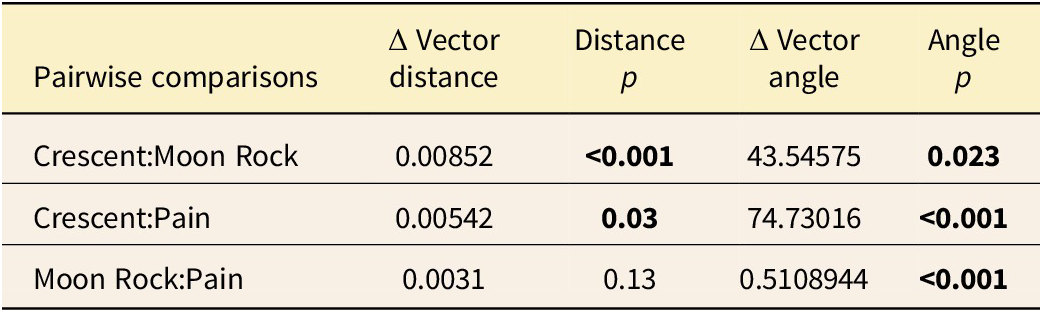
Vector plots from PTA revealed changes in mean shape from dead to live specimens as a vector representing time between time-averaged death assemblages and live-collected individuals (Fig. 8). Pairwise comparisons of vector distances and angles across all model-fit PC axes (not only those illustrated in Fig. 8) indicated that the length of Crescent Pond’s trajectory was significantly different from those of Moon Rock Pond (Z = 3.26, p = 0.003) and Pain Pond (Z = 2.20, p = 0.007) and that trajectory angles were significantly different among all lakes (Table 3). PC 2 represented a shared morphological shift between dead and live specimens in all three lakes from positive to negative means. Dead-to-live trajectories for Moon Rock Pond and Pain Pond have a similar length on PC 1 but their morphology diverged in live populations. In contrast, the trajectory of Crescent Pond, in addition to being longer (i.e., more overall shape changes from dead to living), converged with Pain Pond for living specimens.
Phenotypic shape trajectories between dead (open symbols) and live (filled symbols) specimens from each lake plotted on the first two principal component axes of model-fit coordinate values. Large symbols represent mean shape among each assemblage, with corresponding live (filled) and dead (open) means from each lake connected by line segments that represent the shape-change trajectories. Note that fitted coordinate values used for the trajectory analysis principal component analysis (PCA) are not equivalent to aligned specimen coordinates used to capture total variation, as in Fig. 5.

Figure 8. Long description
A scatter plot with two perpendicular dashed lines intersecting at the origin 0.00, 0.00. The horizontal x-axis is labeled Fitted PC 1 (49.57%) with a scale from -0.03 to 0.03. The vertical y-axis is labeled Fitted PC 2 (30.57%) with a scale from -0.03 to 0.03.
Data points are categorized by three lakes:
* Moon Rock Pond: Represented by purple squares. Small open squares (dead) and filled squares (live) are concentrated in the left half of the plot (negative PC 1). A thick purple line connects a large open square at approximately (-0.01, 0.008) to a large filled square at (-0.014, -0.004), showing a downward-left trajectory.
* Pain Pond: Represented by orange triangles. Small open and filled triangles are concentrated around the center and right-center. A thick orange line connects a large open triangle at (0.001, 0.002) to a large filled triangle at (0.006, -0.007), showing a downward-right trajectory.
* Crescent Pond: Represented by green circles. Small open and filled circles are concentrated in the right half (positive PC 1). A thick green line connects a large open circle at (0.012, 0.009) to a large filled circle at (0.007, -0.011), showing a downward-left trajectory.
A legend in the bottom right corner identifies the symbols for Crescent Pond (green circle), Moon Rock Pond (purple square), and Pain Pond (orange triangle).
Pairwise comparisons of dead-to-live shape trajectories among lakes. Bolded p-values indicate significance following adjustment with the Holm procedure (p < 0.05)

Table 3. Long description
The table consists of five columns: Pairwise comparisons, Delta Vector distance, Distance p, Delta Vector angle, and Angle p.
* Row 1: Crescent to Moon Rock. Delta Vector distance is 0.00852 with a p-value less than 0.001. Delta Vector angle is 43.54575 with a p-value of 0.023.
* Row 2: Crescent to Pain. Delta Vector distance is 0.00542 with a p-value of 0.03. Delta Vector angle is 74.73.016 with a p-value less than 0.001.
* Row 3: Moon Rock to Pain. Delta Vector distance is 0.0031 with a p-value of 0.13. Delta Vector angle is 0.5108944 with a p-value less than 0.001.
Significant p-values (less than 0.05) include both distance and angle for Crescent to Moon Rock, both distance and angle for Crescent to Pain, and only the angle for Moon Rock to Pain.
Diagnostic Shape Differences
Among live-collected specimens, Ctena from Moon Rock Pond were less elongate and had a shortened anterior adductor scar compared with those from Crescent Pond and Pain Pond (Fig. 9A–C). In fact, the relative size of the inhalant channel beneath the anterior adductor scar and detachment of the pallial line (Fig. 2) appears to increase in relative size sequentially from Moon Rock Pond, Crescent Pond, and Pain Pond. Further, a larger mean body size of specimens from Crescent Pond and Pain Pond (Fig. 6A) appears to be associated with a larger relative mantle area compared with specimens from Moon Rock Pond. These patterns were consistent when comparing mean landmark configurations among death assemblages among the three lakes (Fig. 9D–F). When mean dead landmark configurations were compared with their corresponding mean live configurations, two transitions were apparent among all three lakes: (1) the distance between fixed landmarks 2 and 3 (i.e., dorsal and ventral points of the anterior adductor scar; Fig. 2) became shorter, and (2) the marginal shell area exterior to the mantle cavity and pallial line was consistently larger for live-specimen configurations. Thus, both the height of the anterior adductor muscle and the shell area occupied by mantle soft tissue were reduced in life assemblages.
Thin-plate spline (TPS) grids depicting the deformation from the overall mean landmark configuration of the dataset to the mean configurations of life (A–C) and death assemblages (D–F) from Crescent Pond (A, D), Moon Rock Pond (B, E), and Pain Pond (C, F). Deformations are magnified by a factor of four to aid in visualization.

Figure 9. Long description
The figure consists of six panels arranged in a two-by-three grid. Each panel features a warped coordinate grid with a central polygonal landmark outline representing biological shape deformation.
* Top row (Live Assemblages):
* Panel A, Crescent Pond LIVE: The grid shows a slight upward compression on the left and a downward pull on the right.
* Panel B, Moon Rock Pond LIVE: The grid exhibits a distinct inward pinching toward the center-left and a slight expansion on the right.
* Panel C, Pain Pond LIVE: The grid shows a localized downward dip in the upper-right quadrant and a slight upward curve at the bottom-left.
* Bottom row (Dead Assemblages):
* Panel D, Crescent Pond DEAD: The grid is stretched horizontally, with the landmark outline appearing wider and flatter compared to the live counterpart.
* Panel E, Moon Rock Pond DEAD: The grid shows a more uniform compression toward the center, with the landmark outline appearing more compact.
* Panel F, Pain Pond DEAD: The grid displays a wavy deformation pattern, particularly prominent with an upward bulge in the top-left and a downward curve in the top-right.
In all panels, the landmark configuration consists of an outer circular boundary and an inner triangular or wedge-shaped structure on the right side.
These relative mantle area observations were corroborated by quantified internal area ratios (Fig. 10). We found internal area ratios to differ significantly among lakes (F = 31.65, p < 0.001), between life and death assemblages (F = 153.06, p < 0.001), and in the interaction between lake and assemblage (F = 8.15, p < 0.001). Pairwise Tukey tests indicated that death assemblages had relatively greater internal area occupied by the mantle cavity for all lakes, especially for Crescent Pond. Mean area ratios did not differ among lakes for live-collected assemblages, but did for corresponding death assemblages.
Box plot of internal shell area ratios among life and death assemblages from each lake. Ratios were calculated as the area of the semilandmark circle outlining the pallial line (inner mantle area) divided by the area of the semilandmark curve outlining the shell margin (outer margin area).

Figure 10. Long description
The X-axis represents the Internal Area Ratio (Mantle / Margin) ranging from 0.54 to 0.66. The Y-axis is grouped by three lakes, each with a Live and Dead assemblage.
* Crescent Lake (Green): The Live box is centered at approximately 0.59 with whiskers from 0.56 to 0.63. The Dead box is shifted right, centered at 0.625 with whiskers from 0.59 to 0.66 and one outlier at 0.58.
* Moon Rock Lake (Purple): The Live box is centered at 0.585 with whiskers from 0.55 to 0.62 and one outlier at 0.53. The Dead box is centered at 0.61 with whiskers from 0.57 to 0.635 and two outliers near 0.56.
* Pain Lake (Orange): The Live box is centered at 0.60 with whiskers from 0.57 to 0.62 and outliers at 0.54 and 0.64. The Dead box is centered at 0.62 with whiskers from 0.59 to 0.65.
Across all three lakes, the Dead assemblages consistently show a higher median internal area ratio compared to the Live assemblages.
Discussion
The geologically recently established anchialine lakes of San Salvador Island demonstrate an impressive potential for facilitating rapid adaptive radiation as evidenced by endemic pupfishes with specialized feeding morphologies (Turner et al. Reference Turner, Duvernell, Bunt and Barton2008; Chan et al. Reference Chan, Colaco, Martin and Evans2024). Our discovery of thriving populations of chemosymbiotic Ctena in these lakes motivated us to test whether they too diverged morphologically among spatially proximal yet environmentally distinct lakes. By leveraging signals from dead-shell assemblages compared with those from living populations, we aimed to assess possible temporal trends in morphological change both within and among lakes. Our results indicated that (1) shell morphology of live-collected Ctena populations was strongly and significantly distinct among the three lakes, (2) associated dead-collected shells preserved similar among-lake patterns to those observed in the living, and (3) moderate but significant morphological differences were present between living and dead specimens within each lake. The higher share of variation associated with spatial differences among lakes compared with temporal differences between life and death assemblages within lakes suggests that live–dead differences are not associated with changes from an ancestral morphology, but rather, are responses to environmental variation occurring within these habitats.
Spatial Variation and Chemosymbiosis in Anchialine Lakes
To our knowledge, anchialine lakes are a novel habitat type for lucinids like Ctena to thrive in dense populations. Lucinids are important ecosystem engineers in coastal marine biomes like seagrass meadows and mangrove swamps, where they sequester excess carbon and ameliorate sediments of harmful sulfides (van der Heide et al. Reference van der Heide, Govers, DeFouw, Olff, van der Geest, van Katwijk and Piersma2012; Stanley Reference Stanley2014; Martin et al. Reference Martin, Middleton, Fraser, Marshall, Scholz, Hausl and Schmidt2020). However, the small anchialine lakes of San Salvador Island lack extensive vegetation, have thin veneers of sediment above limestone bedrock, and primarily restrict living Ctena to mostly unvegetated or algal-covered karst pockets along the shoreline. It is thus possible that lake-dwelling Ctena have limited and/or differential capacity to perform chemosymbiosis in these lake environments, perhaps even relying more heavily on particulate feeding (Duplessis et al. Reference Duplessis, Dufour, Blankenship, Felbeck and Yayanos2004). Below, we use descriptions of lakebed sediments, pore-water geochemistry, hypothesized environmental conditions, and morphological differences in shells to infer how anchialine environments may have driven plasticity in nutritional strategies (chemosymbiosis vs. particulate feeding) of lake-dwelling Ctena populations (summarized in Table 4).
Summary of lakebed sedimentology, pore-water geochemistry, hypothesized environmental conditions, and Ctena population morphology characteristic to each anchialine lake assessed in this study. Summarized interpretations of lake environmental conditions ("Environmental Characterization") and consequences on chemosymbiosis ("Biological Interpretation") are elaborated on in the “Discussion” section

Table 4. Long description
The table consists of six columns: Lake, Sedimentology, Pore-water geochemistry, Environmental characterization, Ctena morphology, and Biological interpretation.
* Moon Rock Pond: Features white carbonate mud with limited seagrass and low organic content. Geochemistry shows typical marine pH and bicarbonate, high dissolved oxygen, and low sulfide. Characterized as oligotrophic and well-buffered. Ctena are small-bodied with short inhalant channels and low mantle area ratios, interpreted as growth constrained by lower productivity.
* Crescent Pond: Features thick flocculent organic matter over dark carbonate mud with intense lugworm bioturbation. Geochemistry shows low p H, high temperature, high bicarbonate, and high sulfide. Characterized as organic-rich and reducing. Ctena are large-bodied with moderate inhalant channels and high mantle area ratios, interpreted as high growth rates due to high sulfide availability for chemosymbiosis.
* Pain Pond: Features dark carbonate muds with silica sponge spicules and no macrophytes. Geochemistry shows typical marine p H, high dissolved oxygen, and low temperature/conductivity. Characterized as oligotrophic with freshwater dilution and regular oxygenation. Ctena are large-bodied with long inhalant channels and moderate mantle area ratios, interpreted as high growth rates due to oxygen availability and possible reliance on deposit feeding.
Ctena from Moon Rock Pond were characterized by significantly smaller body sizes, shorter detachment of the anterior adductor muscle, and less mantle area demarcated by the pallial line relative to the total shell interior area. Moon Rock Pond may be a more challenging, nutrient-poor habitat for Ctena to facilitate chemosymbiosis and/or particulate feeding, as indicated by its sediment cover of white carbonate mud with few organics and lower measured sulfide concentrations, leading to smaller overall body size driving shape divergence. Although body sizes of different lucinid taxa vary considerably (Taylor and Glover Reference Taylor and Glover2009; Anderson Reference Anderson, Hembree, Platt and Smith2014), intraspecific population-level body-size responses to organic matter concentrations have been documented in other species. For example, increased body size for the Pacific taxon Parvilucina tenuisculpta in Southern California corresponded to high levels of municipal waste effluent off the coast of Los Angeles during the 1970s (Fabrikant Reference Fabrikant1984), and seasonal food limitation in the tropical seagrass-associated Loripes orbiculatus (identified at the time as L. lucinalis) was observed to correlate with size-corrected body and somatic mass changes (van der Geest et al. Reference van der Geest, Sall, Ely, Nauta, van Gils and Piersma2014). A particularly oligotrophic environment at Moon Rock Pond could thus result in a resident population experiencing slower growth and/or reduced maximum body size relative to the other two lakes (e.g., Morton et al. Reference Morton, Da Cunha and De Frias Martins2014; Fuksi et al. Reference Fuksi, Tomašových, Gallmetzer, Haselmair and Zuschin2018).
Ctena from Pain Pond exhibited longer and more detached anterior adductor muscles, resulting in a relatively enlarged inhalant channel. This increased detachment and lengthening relative to Ctena from Crescent Pond, while maintaining a similar overall centroid size, is consistent with Pain Pond Ctena having a steeper allometric slope of shape change with growth (Fig. 6). Such a morphological signature could be in response to higher pore-water dissolved oxygen concentrations we observed at Pain Pond, facilitating faster growth rates. Numerous studies have demonstrated strong allometric relationships between body size and gill area/biomass, which in turn correlate with faster respiration and clearance rates (Järnegren and Altin Reference Järnegren and Altin2006; Le et al. Reference Le, Alfaro, Ibarrola, Ragg, Hilton and King2017), and lucinids use their inhalant channel to draw in water from the sediment–water interface and facilitate respiration while living at depths with poor oxygen availability (Stanley Reference Stanley1970; Taylor and Glover Reference Taylor and Glover2009; Anderson Reference Anderson, Hembree, Platt and Smith2014). Alternatively, greater investment in the inhalant channel could indicate a greater reliance on particulate deposit feeding in the relatively deep karst pockets of Pain Pond with no vegetative cover (Duplessis et al. Reference Duplessis, Dufour, Blankenship, Felbeck and Yayanos2004).
Ctena from Crescent Pond had the greatest relative proportion of surface area interior of the pallial line (Fig. 10), with which they could house larger gills with more bacteriocytes, and thus increase the density of endosymbionts as similarly observed in chemosymbiotic Bathymodiolus mussels (family Mytilidae; Duperron et al. Reference Duperron, Quiles, Szafranski, Léger and Shillito2016). Van der Geest et al. (Reference van der Geest, van der Heide, Holmer and de Wit2020) similarly reported that L. orbiculatus populations associated with seagrass meadows on the southern coast of France experienced increased flesh/shell dry weight ratios when increased organic matter and sulfide levels were experimentally introduced. Because Crescent Pond had higher pore-water dissolved sulfide concentrations, intense bioturbation from resident annelids, and a thick layer of flocculent organics on the lakebed, chemosymbiosis is perhaps efficiently facilitated by Ctena in this lake environment compared with Moon Rock Pond and Pain Pond. Low pH at Crescent Pond suggests that such rates of organic decomposition and sulfate reduction make this lake particularly productive, but also result in conditions that are weakly buffered from changing acidity, which may harm resident bivalves and decrease time averaging of death assemblages (see next subsection).
This study demonstrates that morphological features relevant to chemosymbiosis of lucinid bivalves are impressively plastic to environmental conditions over both space and time. Because lake-dwelling Ctena exhibited strong differences in phenotypic traits correlated with a chemosymbiotic lifestyle, and because these geologically young lakes exhibited sedimentological and geochemical characteristics distinct from one another, observed spatial variation is likely driven by ecophenotypic plasticity to the environmental conditions of each lake. Indeed, bivalves elsewhere have demonstrated a profound capacity for phenotypic plasticity in response to new environmental conditions, including variable growth rates and shell shape divergence (McLachlan et al. Reference McLachlan, Jaramillo, Defeo, Dugan, de Ruyck and Coetzee1995; Valladares et al. Reference Valladares, Manríquez and Suárez-Isla2010; Sharma et al. Reference Sharma, Mondal, Ganguly and Giri2023; Alma et al., Reference Alma, McElhany, Crim, Newton, Maher, Mickett and Padilla-Gamiño2024; Keogh et al. Reference Keogh, Minerich, Ohlman, Pletta, Scheunemann, Schroeder, Secrist, Franzen, Sietman and Simons2025; Osei et al. Reference Osei, Yankson and Obodai2026). Employing a similar landmark configuration as that used in this study, Anderson et al. (Reference Anderson, Long-Fox, Paterson and Engel2022) found that morphological variation in the lucinid Stewartia floridana tracked seagrass coverage and stability in a single seagrass meadow in western Florida, demonstrating the sensitivity of lucinid morphology to fine-scale environmental gradients, even without geographic isolation.
Temporal Variation and Environmental Fragility of Lakes
Lake-dwelling Ctena exhibited relatively modest morphological change between life and death assemblages (relative to differences among lakes), and the trajectories of mean dead to mean live shell shape were significantly different in both magnitude and direction among lakes (Fig. 8, Table 3), making temporal shifts in morphology unique for each population. That said, life assemblages at each lake exhibited less mantle area interior of the pallial line relative to total shell area compared with death assemblages, suggesting that some aspects of temporal shape change were shared among lakes. Assuming that lake-dwelling Ctena descended from a single metapopulation sourced from the coastal seabeds around San Salvador Island, dead-to-live trajectories are likely to represent recent morphological changes that postdate geographic isolation and morphological divergence among lake populations. Our collection of articulated specimens with both valves further enables us to pursue subsequent investigations of fluctuating asymmetry as an indicator of developmental instability, which bivalves have previously demonstrated to exhibit when facing thermal stress (Nishizaki et al. Reference Nishizaki, Barron and Carew2015), industrial pollution (Scalici et al. Reference Scalici, Traversetti, Spani, Malafoglia, Colamartino, Persichini, Cappello, Mancini, Guerriero and Colasanti2017), and intertidal habitats (Trivellini et al. Reference Trivellini, Van der Molen and Márquez2018); this dimension of Ctena morphometrics is actively being investigated.
Because temporal variation in shell morphology among lake-dwelling Ctena postdated allopatric divergence among lakes, and because death assemblages were not reliably indicative of the ancestral morphology at the time of colonization, differences between life and death assemblages are likely driven by changing or variable environmental conditions of sensitive anchialine habitats. Indeed, numerous marine bivalve taxa physiologically respond to stressors common to lakes, such as heat waves (Masanja et al. Reference Masanja, Yang, Xu, He, Liu, Xu and Xiaoyan2023; Chen et al. Reference Chen, Zhou, Zheng, Hu, Kong, Zhao and Dong2024), salinity fluctuations (Peteiro et al. Reference Peteiro, Woodin, Wethey, Costas-Costas, Martínez-Casal, Olabarria and Vázquez2018), acidification (Stevens and Gobler Reference Stevens and Gobler2018), and compounding effects of multiple stressors (Genovese et al. Reference Genovese, Hudon, Martel and Cattaneo2016; Welton et al. Reference Welton, Hoppit, Schmidt, Witts and Moon2024; Rynkowski et al. Reference Rynkowski, Ellis, Needham and Pilditch2025). Morphological shifts between dead- and live-collected Ctena could thus serve as a proxy for environmental stability of these lakes, similar to how Anderson et al. (Reference Anderson, Long-Fox, Paterson and Engel2022) found live–dead discordance in morphology of S. floridana to serve as a proxy for seagrass stability in a marine coastal meadow.
Although somewhat environmentally buffered by subsurface connections to adjacent coastal areas, anchialine lakes are recognized for compounding sensitivities to changes in atmospheric, terrestrial, and oceanic conditions (Mejía-Ortíz et al. Reference Mejía-Ortíz, Chávez-Solís and Brankovits2022). Compared with open-marine seabeds or large ancient lakes, small and shallow lacustrine ecosystems are susceptible to environmental perturbations that include rising temperatures, altered precipitation, intensifying storms, and direct human disturbance (Jeppesen et al. Reference Jeppesen, Meerhoff, Davidson, Trolle, Sondergaard, Lauridsen and Beklioğlu2014; Havens et al. Reference Havens, Paerl, Phlips, Zhu, Beaver and Srifa2016; Woolway et al. Reference Woolway, Jennings, Shatwell, Golub, Pierson and Maberly2021). The resilience of these habitats to changing climate dynamics is particularly dubious in the Bahamas, where atmospheric temperature, precipitation, and evapotranspiration are highly variable from year to year among island nations in the Caribbean (Spellman et al. Reference Spellman, Pritt and Salazar2021). It is thus possible that temporal trends in Ctena morphological variation might signal ongoing changes to the complex web of environmental interactions that affect lacustrine habitats.
Caveats and Utility for Live–Dead Comparisons
In using dead-collected shells to detect potential temporal patterns in morphological variation, it is important to consider the duration and structure of time averaging they represent. Our collection of only articulated dead shells from the top ~30 cm of sediment aimed to minimize the possibility of postmortem transport, ensuring specimens were more likely sampled from their life positions (Stanley Reference Stanley2014). In excluding disarticulated specimens, however, we almost certainly truncated the duration of time averaging represented by our death assemblages (Kidwell Reference Kidwell2013). Nevertheless, our detection of morphological differences between live- and dead-collected Ctena suggests that time averaging is sufficient to detect ongoing changes in shell morphology from a time-averaged baseline. Indeed, our results contrast with similar studies that found no differences in mean shape between living and dead specimens in open-marine systems that are more time averaged (e.g., Bush et al. Reference Bush, Powell, Arnold, Bert and Daley2002; Krause Reference Krause2004). Rather, this study corroborates findings by more recent work that live–dead comparisons can be used to detect morphological variation associated with fine-scale environmental gradients (e.g., Huntley et al. Reference Huntley, Schiffbauer, Avila and Broce2018; Anderson et al. Reference Anderson, Long-Fox, Paterson and Engel2022; Abdelhady et al. Reference Abdelhady, Husain, Samy-Kamal, Ahmed, Alexakis and Ali2023).
The addition of radiocarbon-calibrated postmortem age data could “age-unmix” death assemblages to assess both the duration of time averaging and the rate of morphological changes observed in this study (e.g., Tomašových and Kidwell Reference Tomašových and Kidwell2017; Agiadi et al. Reference Agiadi, Azzarone, Hua, Kaufman, Thivaiou and Albano2021). Although our lake-dwelling dead Ctena shells have not yet been dated in this way, there have been such studies performed on San Salvador Island. Kowalewski et al. (Reference Kowalewski, Casebolt, Hua, Whitacre, Kaufman and Kosnik2018) found that shells of the bivalve Tucetona pectinata along the western coast had a mean radiocarbon age of ~1300 years, with the oldest sampled shell being ~4300 years. Terrestrial plant leaves in cores from the hypersaline Storrs Lake, a large lake on the eastern side of the island, were dated to ~40–60 years in the core’s top 1 cm (Park Reference Park2012). Using these estimates, Michelson et al. (Reference Michelson, Kidwell, Boush and Ash2018) inferred that ostracods from San Salvador’s blue holes and anchialine lakes are likely time-averaged on a scale of multiple decades but that an appreciable number of specimens from previous centuries could be intermixed. With dead-collected specimens archived at SDSM, future investigations could evaluate how time averaging varies among populations from the three anchialine lakes.
Another important taphonomic caveat is that dead-collected specimens could have been altered postmortem, and this might affect landmark placement (Webster and Sheets Reference Webster, Sheets, Alroy and Hunt2010; Kammerer et al. Reference Kammerer, Deutsch, Lungmus and Angielczyk2020). Internal faces of dead-collected lucinid shells are generally more opaque, making the outlines of adductor scars and pallial lines easier to discern in photographs (see Anderson et al. Reference Anderson, Long-Fox, Paterson and Engel2022: fig. 3). Postmortem alteration may (1) reduce human error in placing landmarks and/or (2) lead to taphonomic alteration of landmark positions. We believe the first scenario is not playing a role for our Bahamian dataset, because human errors would likely lead to increased shape variation of life assemblages. Instead, our results indicated the life assemblages had similar amounts of variation as their corresponding death assemblages (e.g., convex hulls in Fig. 5). We also believe the second possibility is not an issue, because our dead-to-live trajectories indicated significant differences in both distance and angle, meaning that the nature of morphological change between dead and living is independent among lakes. That said, absolute age dating could reveal many dead-collected specimens to be exceptionally young (e.g., less than a few years or decades). Such a short window of time averaging would support explanations for our live–dead differences to be driven by postmortem alterations.
Most live–dead comparison studies evaluate taxonomic compositions or ecological metrics (richness, evenness, etc.) where long-term monitoring data are lacking (e.g., numerous examples from San Salvador Island; Yanes Reference Yanes2012; Casebolt and Kowalewski Reference Casebolt and Kowalewski2018; Michelson et al. Reference Michelson, Kidwell, Boush and Ash2018; Brown and Larina Reference Brown and Larina2019). However, an increasing number of studies incorporate morphometric data to understand how populations have responded to environmental changes (Krause Reference Krause2004; Lockwood and Mann Reference Lockwood and Mann2019; Anderson et al. Reference Anderson, Long-Fox, Paterson and Engel2022; Abdelhady et al. Reference Abdelhady, Husain, Samy-Kamal, Ahmed, Alexakis and Ali2023). With the formalization of conservation paleobiology as a field of study, morphometric comparisons between life and death assemblages are thus powerful tools for detecting shifting baselines due to recent environmental changes and/or anthropogenic impacts.
Discerning Adaptive versus Ecophenotypic Divergence
Is the ecophenotypic spatiotemporal variation observed for lake-dwelling Ctena indicative of an ongoing adaptive radiation? Current evidence suggests that these populations instead represent an early stage of divergence in which substantial morphological differentiation has emerged despite little detectable phylogenetic structure (Long-Fox et al. Reference Long-Fox, Anderosn, Lim, Campbell, Kokesh, Paterson and Engel2025). Phenotypic plasticity to environmental heterogeneity is increasingly recognized as a precursor to subsequent genetic divergence (Muschick et al. Reference Muschick, Barluenga, Salzburger and Meyer2011; Fitzpatrick Reference Fitzpatrick2012; Schneider and Meyer Reference Schneider and Meyer2017; Parsons et al. Reference Parsons, McWhinnie, Pilakouta and Walker2020). This pattern suggests either (1) recent colonization relative to the perennial establishment of these lakes during the ~6–10 ka of the Holocene transgression (Hagey and Mylroie Reference Hagey, Mylroie, Curran and White1995; Teeter Reference Teeter, Curran and White1995; Turner et al. Reference Turner, Duvernell, Bunt and Barton2008) or (2) morphological divergence proceeding more rapidly than genome-wide differentiation. Because death assemblages likely encompass a timescale more recent than initial colonization, integrating genomic and paleoecological perspectives will be critical for determining whether these ecophenotypic differences represent persistent plastic responses or the incipient stages of adaptive divergence.
Data Availability Statement
Data and code used in this study are available on Dryad at https://doi.org/10.5061/dryad.nk98sf88k.
Acknowledgments
We thank T. Dexter and the staff at the GRC for logistical support and accommodations on San Salvador Island. We also thank Z. Payne, A. Tran, and C. Fortier for assistance in the field and the laboratory. This research was conducted with approval by the following Bahamian institutions: The Bahamas Environment, Science, and Technology (BEST) Commission, the Antiquities, Monuments, and Museums Corporation (AMMC), The Bahamas National Trust (BNT), the San Salvador National Parks System, and The Bahamian Ministry of Agriculture. Funding was provided by the National Science Foundation (DEB-1342721 to L.C.A. and DEB-1342785 to A.S.E.) and student grants to B.S.K. from the Geological Society of America and Conchologists of America.
Author Contribution
B.S.K. and L.C.A. designed the study; A.S.E. and L.C.A. acquired funding; B.S.K. and B.L.L.-F. conducted specimen-based morphometric analyses; A.T.P. and A.S.E. analyzed geochemistry data; B.S.K. completed data analysis and visualizations; all authors contributed to fieldwork; B.S.K. wrote the paper; all authors contributed to and approved the final version of the submitted manuscript.
Competing Interests
The authors declare no competing interests.






 Open access

