Quiescent and active nuclei

A quiescent cell can be described as not being involved in growth or division, although other functions generally may continue as usual. By extension, a quiescent nucleus is defined as one that does not contribute to an increase in cell mass or cell division, that is, a nucleus for which the associated synthesis (PS) and breakdown (PB) rates of protein are equal (i.e. PS = PB). In contrast, an active nucleus can be defined as one that contributes to an increase in cell mass or number (i.e. PS > PB).

Let α be the amount of body or tissue protein at maturity, so that (P/α) can be regarded as the degree of protein maturity. For a quiescent nucleus, I assume that PS = PB ∝ (P/α)^X, with the sign ∝ meaning ‘proportional to.’ The power X represents the rate-limiting step in breakdown rate and it is possibly unequal to zero to allow for changes in breakdown control associated with age or size due to genetic, diet or other factors. It can also be assumed that the number of nuclei (nn) in a tissue scales with protein amount proportional to a power Z, nn ∝ (P/α)^Z. With all nuclei in a tissue in the quiescent state, PS and PB will scale as

(2)

with c a constant of proportionality and PS and PB measured in kg/day.

In general, whole body or skeletal muscle nn ∝ (P/α)^2/3, that is, Z = 2/3 (Roux, Reference Roux2006). To accommodate tissues with multinucleate cells, like muscle, a DNA unit will be defined as having a mass of P/nn ∝ (P/α)^1/3. For tissues with mononucleate cells, a DNA unit will be identical to a cell. It follows that the diameter of a whole body or skeletal muscle DNA unit will scale ∝(P/α)^1/9, surface area ∝(P/α)^2/9, and from Fick’s law the diffusion capacity is proportional to surface/distance = (P/α)^2/9/(P/α)^1/9 = (P/α)^1/9. Hence, specific diffusion capacity for a DNA unit is proportional to (P/α)^1/9/(P/α)^1/3 = (P/α)^−2/9, with specific surface area being proportional to (P/α)^2/9/(P/α)^1/3 = (P/α)^−1/9.

Control of breakdown rate

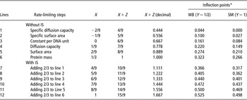
For the purpose of growth description, it is perhaps important to distinguish between quantitative and qualitative control. Qualitative control would refer to the control of the breakdown of different types of protein, whereas quantitative control refers to the total amount of degraded protein. The total degradation rate would therefore be dependent on the concentration of the elements of the degrading system, which consists of lysosomes as well as a pathway inside the cytoplasm often adjacent to plasma or other membranes. It is therefore logical to expect that total protein breakdown would be related to cell or DNA unit mass, surface area or diffusion capacity. The scaling of the different possibilities for the rate-limiting step in breakdown rate (equation 2) is given in Table 1. They follow directly from the preceding discussion on DNA unit scaling. The whole body or skeletal muscle power Z is assumed to be equal to 2/3 (Roux, Reference Roux2006). In line 1 (Table 1), it is assumed that the rate-limiting step for breakdown rate is proportional to the specific diffusion capacity for each DNA unit, that is, to (P/α)^−2/9, so that X = −2/9 and X + Z=4/9 for total specific diffusion capacity. The argument for the derivation of lines 2 to 6 in Table 1 is analogous to that for line 1.

Table 1

The WB or SM powers X + Z associated with different rate-limiting steps without and with IS for protein breakdown rate together with inflection points from equation (9)

WB = whole body; SM = skeletal muscle; IS = intercellular signaling.

*The inflection point is in terms of protein maturity (P/α); X, the power representing the rate-limiting step in protein breakdown associated with a single nucleus; Y, the power in the relationship between cell volume and the amount of protein in a tissue or the WB; Z, the power in the relationship between the number of nuclei and the amount of protein in a tissue or the WB.

To obtain lines 7 to 12, PB regulation by paracrine or intercellular signaling is assumed in addition to the rate-limiting steps indicated in lines 1 to 6, in such a way that the magnitude of the effect on PB in a DNA unit is proportional to the total number of nuclei in a tissue. Lines 7 to 12 can then be obtained by increasing X in lines 1 to 6 by 2/3, the power in the relationship nn ∝ (P/α)^2/3. The inflection points in Table 1 will be discussed later .

For cells classified as viscera, skin or bone, separate values obtained from Roux (Reference Roux2006) indicate that Z ≠ 2/3. Hence, different but analogous tables of both X and Z will have to be constructed for them on the basis of Z = 5/6 (viscera) or Z = 1/2 (skin or bone; see Tables A1 and A2 in Roux (Reference Roux2010)).

Protein synthesis

In the same way as protein breakdown, the control of PS can be differentiated into qualitative and quantitative control. Qualitative control refers to the composition of synthesized proteins that is mediated by the initiation of transcription by promoters. Quantitative control, with reference to the rate of PS, mainly depends on activators bound to DNA sequences called enhancers. Generally, the control of the rate of PS would therefore depend on activator concentration in the nucleus (Roux, Reference Roux2005a). Activator precursors will have to diffuse into the nucleus. Let nv denote nuclear volume. The nuclear surface will scale proportionally to (nv)^2/3 and nuclear diameter to (nv)^1/3. Then, from Fick’s law, diffusion rate into the nucleus will be proportional to the concentration gradient and diffusion capacity, with specific diffusion capacity = (surface/distance)/volume = [(nv)^2/3/(nv)^1/3]/nv = (nv)^−2/3. Assume that for activator precursors the signaling cascade through the cytoplasm always contains such a number of steps that the activator precursor concentration in the cytoplasm does not vary with cell size. On the basis of this premise, it is reasonable to accept that the concentration gradient of activator precursors will be invariant with cell size and hence with time. Then, if activator lifetime is also constant during growth, activator concentration will be proportional to specific diffusion capacity (Roux, Reference Roux2005a):

(3)

It can be assumed that the rate of PS depends essentially on the rate of gene transcription (Latchman, Reference Latchman2005). It is also reasonable to expect that the specific rate of gene transcription would be proportional to the concentration of activators bound to enhancers. Analogous to hormone-binding kinetics (Darnell et al., Reference Darnell, Lodish and Baltimore1990), this activator–enhancer complex concentration would, in turn, be proportional to activator concentration. The rate of gene transcription per nucleus will then be determined by the activator concentration in equation (3) (Roux, Reference Roux2005a). Furthermore, age- or size-related effects (age or size changes ∝(P/α)^X), as in equation (2), are also applicable to all nuclei. Then for the total rate of PS (kg/day) with all nuclei (nn ∝ (P/α)^Z) in a tissue activated by a cascading effect obtained from hormonally mediated growth factors bound to receptors on the cell surface, it follows from equation (3) (Roux, Reference Roux2005a and Reference Roux2006) that

(4)

From Teissier (Reference Teissier1941), it generally holds for mammalian cells that nuclear volume is proportional to cell volume (cv), such that nv ∝ (cv)^2/3. If it is assumed that cv is related to a power Y of the P/α of a tissue, such that cv ∝ (P/α)^Y, equation (4) becomes

(5)

The constants c in equations (2) and (5) are equal, since at maturity (P/α) = 1 and PS = PB.

The assumptions used in the derivation of equation (5) do not seem to allow a gradient of responses for an active nucleus. For differential growth in a tissue, it is therefore assumed that the differential protein growth response elicited by hormonal control is obtained by variation of the proportion of active nuclei in a tissue. Let Q denote the proportion of active nuclei in a tissue. Then, from the addition of active (equation 5) and quiescent nuclei (equation 2), a tissue will have a total synthesis rate of

(6)

Protein retention

Since PR = PS−PB, the equation for PR (kg/day) can be obtained from the difference between equations (6) and (2):

(7)

PR can be taken to be equal to the differential dP/dt, which will allow equation (7) to be regarded as a differential equation that can be solved for P, the amount of protein in a tissue. The differential equation associated with equation (7) does not have an analytic solution for all powers of (P/α). Values for the powers of (P/α) for which analytic solutions exist, together with the solutions, are published in Reiss (Reference Reiss1989). For example, for X + Z = 1 the solution of equation (7) is

(8)

(von Bertalanffy, Reference von Bertalanffy1960) with P ₀ representing the amount of protein in a tissue at time zero, h = (4/9)Y and k = ch(Q/α). Equation (7) has to be solved numerically for values of X + Z for which no analytic solution exists.

The cellular or physiological basis of protein growth parameters

Note that a cellular or physiological basis exists for all the parameters of equations (7) and (8). The limit or mature protein mass in equations (2) and (4) can be shown to arise from the relationship between PS and PB described by the parameterization of equation (1), namely α = (c ₂/c ₁)^1/(a−b) (Roux, Reference Roux2005a). The explanation of the power of the whole body breakdown rate X + Z is encompassed in Table 1. The constant 4/9 arises from the scaling of the specific diffusion rate of activator precursors from nuclear dimensions and from the relationship between nuclear volume and cell volume. The parameter Y is the power of the relationship between cell volume and amount of tissue protein. The number of multinucleate muscle cells does not increase after birth, so that Y = 1 for skeletal muscle (Roux, Reference Roux2006). On the basis of DNA–protein relationships, it is derived by Roux (Reference Roux2006) that Y = 1/3 for mononucleate cells on average, with Y = 1/6 for viscera and Y = 1/2 for both skin and bone. For the whole body, the contribution of the different tissues should be weighed in proportion to their PS rates. On average, Y = 1/2, approximately, for the whole body (Roux, Reference Roux2006).

Point of inflection

Expressed in terms of protein maturity, the protein mass at the point of inflection of equation (7) is as follows from von Bertalanffy (Reference von Bertalanffy1960)

(9)

The values of P/α at the inflection point for whole body Y = 1/2 and skeletal muscle Y = 1 are given in Table 1 for the different postulated values of X + Z.

Evidence for the postulated values of Y

The first question that needs to be answered here is whether equation (7) with theoretical average Y = 1/2 for whole body protein can explain the range of experimental results recorded in the literature. Evidence in confirmation of Y = 1/2, together with (4/9)Y = 2/9, from PS or retention efficiency experiments for pigs, cattle and sheep as well as a weighted average from different tissues is available from Roux (Reference Roux2005a, Reference Roux2005b and Reference Roux2006). In this approach, problems with the separate estimation of a or b in equation (1) were largely ignored, with attention instead focused on estimation of the difference a−b.

As in the present approach, Oltjen et al. (Reference Oltjen, Bywater and Baldwin1985) also modelled PR in terms of PS and PB. With reparameterization, their results provide evidence in favor of the present approach. On account of the generally high correlation between estimates of its parameters, it is difficult to obtain a direct fit to equation (1) by the conventional methods of estimation of a and b. Oltjen et al. (Reference Oltjen, Bywater and Baldwin1985) circumvented the problem by using an independent estimate of protein breakdown to obtain an estimate of PS from the rat data of Enesco and Leblond (Reference Enesco and Leblond1962). By adding PB to PR to obtain PS, they effectively obtained equation (7), if Q = 1 is assumed. Transposed to the present notation, Oltjen et al. (Reference Oltjen, Bywater and Baldwin1985) assumed X + Z = 0.72 and estimated X + Z−(4/9)Y = 0.48. Solving this gives Y = 0.54, near to the average value derived by Roux (Reference Roux2006). Oltjen et al. (Reference Oltjen, Bywater and Baldwin1985) also estimated PS ∝ (DNA)^0.72 from birth onward and PS ∝ (DNA)^0.75 from weaning onward. Taking DNA ∝ P ^2/3(derivation of equation 2), this gives PS ∝ P ^0.48(0.48 = 0.72 × 2/3) as before from birth onward, but PS ∝ P ^0.50(0.50 = 0.75 × 2/3) from weaning onward. This gives X + Z−(4/9)Y = 0.50 and with the Oltjen et al. (Reference Oltjen, Bywater and Baldwin1985) assumption of X + Z = 0.72, it follows that Y = 0.50 identical, from weaning onward, to the value suggested by Roux (Reference Roux2006).

Confirmation derived from experimental estimates of PS and PB for the theoretical estimates of Y = 1 (muscle), Y = 1/2 (skin or bone), Y = 1/6 (viscera) and 1/3 (average for mononucleate cells) is available in Roux (Reference Roux2006).

Di Marco et al. (Reference Di Marco, Baldwin and Calvert1989) aggregately considered two protein pools: body and viscera. Body consisted mainly of skin, muscle and bone; viscera included blood, liver, digestive tract, heart and lungs. When Di Marco et al.’s (Reference Di Marco, Baldwin and Calvert1989) descriptions by complex equations of body and viscera were approximated by equation (1), values of a−b = 0.324 for the body and a−b = 0.078 for the viscera were obtained in reasonable agreement to theoretical expectations of 0.296 and 0.074 derived from weighted synthesis contributions from the viscera, skin or bone and skeletal muscle (Roux, Reference Roux2006).

The tenability of the derived range of theoretical X + Z powers

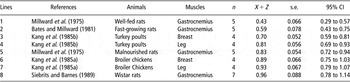
An alternative approach to the estimation of parameters of equation (7) is via its components PB (equation 2) and PS (equation 6). Unless Q is known and equal to 1, equation (6) will be difficult to fit, for the same reason as equation (1). To this will be added the additional problem that, due to measurement difficulties, the available experimental observations tend to be concentrated at few points. Hence, iterative methods may fail to converge or may result in poor estimates and therefore no attempt will be made to fit equation (6). In contrast, equation (2) is easy to fit with linear regression under logarithmic transformation. This will provide valuable evidence on the tenability of the theoretically predicted values of X + Z in Table 1. Estimates from equation (2) of the powers of the whole body protein breakdown rate X + Z are in Table 2 and those of the powers of muscle breakdown rate X + Z are in Table 3.

Table 2

The WB estimates of the powers of protein breakdown rate X + Z together with 95% CI from regression coefficient estimates obtained by logarithmic transformation according to equation (2) on protein breakdown data from the literature

WB = whole body.

Table 3

The muscle estimates of the powers of protein breakdown rate X + Z together with 95% CI from regression coefficient estimates obtained by logarithmic transformation according to equation (2) on protein breakdown data from the literature

F-test for heterogeneity: F = 9.81^xx with 7 and 22 d.f.

The confidence intervals in Table 2 for the powers of the whole body breakdown rate indicate that the mammalian observations are in agreement with the theoretical value of X + Z=6/9 in Table 1, whereas the chicken value is indicated to be in agreement with values of 8/9 to 10/9.

Applied to the values of X + Z for muscle in Table 3, an F-test for heterogeneity of regression coefficients indicates significance at the 0.01 level with F = 9.81 with 7 and 22 d.f. To get enough degrees of freedom for reliable confidence intervals of the regression coefficients, a common standard deviation from regression of 0.1558 with 22 d.f. was calculated.

Note that for muscle the significant heterogeneity F-value together with non-overlapping confidence intervals indicates that no single theoretical value of X + Z in Table 1 can explain the observed values in Table 3. Instead, agreement to the whole range of values in Table 1 from lines 1 to 6 is indicated, with each estimate in Table 3 an s.e. or less away from a theoretical value in Table 1. The only difference between the well-fed rats (line 1) and the marginally malnourished rats (line 5) from the same laboratory is in the dietary protein concentration of their food, indicating that nutritional influences may cause significant differences in the observed values of X + Z. In contrast, the significant difference between the slow-growing well-fed rats in line 1 as well as the fast-growing rats in line 2 with the Wistar rats in line 8 suggests the importance of genetic differences in observed X + Z-values.

Tables 2 and 3 do not provide any evidence for X + Z-values substantially above unity. With X + Z = 1, the maximum value of the point of inflection is the Gompertz value of P/α = 0.368 with Y→0. However, fitting a Bridges curve with a flexible point of inflection, Knap (Reference Knap2000) obtained values for the inflection point on modern pig protein growth data, given in Table 4, with inflection points showing an increasing trend above the Gompertz value. On the assumption of Y = 1/2, equivalent inflection points from equations (7) and (9) will require values of X + Z substantially above unity. Consequently, the observations in Table 4 are in agreement with lines 7 to 10 in Table 1.

Table 4

Time trends in inflection points obtained by Knap (Reference Knap2000) on protein growth data for modern pigs together with the powers of protein breakdown rate X + Z that would result in equal inflection points from equation (9) under the assumption of Y = 1/2

Y, the power in the relationship between cell volume and the amount of protein in a tissue or the whole body.

In evaluating the information in Table 4, it is important to realize that the 1976 population represents unimproved pigs before the initiation of modern selection programs. It therefore gets the first position in the improvement time rank. The 1969 values represent one of the first populations to be systematically selected for growth and body composition traits and therefore gets the second improvement time rank. The values for 1984, 1990 and 1993 represent pigs with greater periods of improvement from their populations of origin behind them, and therefore obtain larger time ranks. The X + Z rankings represent the magnitude of the numerical values of X + Z. Note that the two rankings are in complete agreement. This corresponds to a Spearman’s rank correlation coefficient of unity, r_s = 1. With n = 5, r_s = 1 is significant for a one-tailed test at the 0.01 level of significance. This means that the trend in X + Z with time due to breeding improvement is not likely to be a chance event. The likely proximate cause of larger X + Z values is that breeding improvement causes faster growth at more advanced ages in improved pigs compared with unimproved ones, indicating the importance of genetic influence on the point of inflection.

The general conclusion follows that Tables 2 to 4 provide substantial experimental support for the range of the theoretical values of X + Z postulated in Table 1. This means that a whole range or family of protein growth curves exists for mammals given by equation (7) with postulated values of X + Z like Table 1 and values of Y according to the type of tissue or whole body tissue composition.

The interpretation and estimation of Q

From equation (7), it is evident that, other things being equal, the maximum PR will occur with Q = 1, that is, with all nuclei in the active state. Experimental evidence for the existence of a maximum PR (PR_max) is summarized by Moughan (Reference Moughan1999). In growing pigs, several hyperalimentation studies indicate that the supply of a balanced diet at a level exceeding normal ad libitum ingestion leads to an increased growth rate, but not an increased retention of body protein. These studies imply the operation of a maximal rate of PR (Moughan, Reference Moughan1999).

At present, no method exists for the direct estimation of Q. Indirect estimates have therefore been devised by Roux (Reference Roux2005a and Reference Roux2006) to comply with the basic property of a proportion, that is, to vary between zero and one. Here, a generalization will be presented, derived from a theory developed for pigs (Kyriazakis and Emmans, Reference Kyriazakis and Emmans1992) that contains Roux’s (Reference Roux2005a and Reference Roux2006) formula based on intake rate as a simplification applicable to protein-limiting foods.

From equation (7), it follows that PR = QPR_max, or Q = PR/PR_max. From Sandberg et al. (Reference Sandberg, Emmans and Kyriazakis2005), PR = e_P(IPI−IPM), with IPI indicating ideal protein (IP) intake and IPM indicating IP intake at protein maintenance when PR = 0. Kyriazakis and Emmans (Reference Kyriazakis and Emmans1992) made the marginal efficiency of retaining IP (e_p), a function of the ratio of the metabolizable energy (ME) content (MEC, MJ/kg), to the digestible crude protein (DCP) content (DCPC, kg/kg) of the food, R (MJME/kgDCP). The proposed relationship is e_P = μR, with μ a constant and a maximum value for e_P of when R is above a specific value R*. With this notation, (IPO−IPM), with IPO the optimal IPI when PR = PR_max. It follows that

(10)

Two special cases of equation (10) are of interest. The first is for protein-limiting foods when R > R* and consequently , so that

or for PR and PR_max on different levels of the same diet

(11.1)

with MEM the ME intake at body protein maintenance and MEO the ME intake at PR_max, since on levels of the same diet the ratios involving IP and ME will be the same.

Equation (11.1) is identical to the estimate previously suggested by Roux (Reference Roux2005a). An estimate based on insulin-like growth factor (IGF) concentration in the blood is similar with (IGF) replacing ME. For energy-limiting foods when R > R* equation (10) or an ME equivalent will have to be used, with , equation (11.1) will overestimate Q.

The second special case of interest from equation (10) is when R > R*, but the levels of IPI on the different diets are the same and equal to IPO. The last term of equation (10) then cancels so that it becomes

(11.2)

as follows from the definition of R. Experimental evidence for the validity of equation

follows from the approximate linear relationship between PR and MEI with zero intercept for pigs between 45 and 100 kg live mass and MEI of 0.7, 0.8, 0.9 and 1.0 × MEO, with approximate constant CPI, obtained by Quiniou et al. (Reference Quiniou, Dourmad and Noblet1996).

For cattle (Roux, Reference Roux2005b), the available evidence on the application of equation (11.1) indicates Q = 1 in equation (7) at ad libitum intake on diets adequate for maximal growth. In contrast, some evidence exists for sheep (Roux, Reference Roux2005b) that either Y < 1/2 or Q < 1 at ad libitum intake, except for compensatory growth during realimentation after diet restriction. The application of equation (11.1) is illustrated in Roux (Reference Roux2005b) for cattle and sheep.

General protein growth curves for mammals

In Table 2, the average value for X + Z for mammals is near to 2/3. Since none of them is significantly different from 2/3, equation (2) can be fitted for each species for PB and by calculating α according to the formulas in Roux (Reference Roux2005a). The constant c, calculated by assuming X + Z=2/3, together with α is as follows

A logarithmic regression of c on α gives a slope of 0.768 (s.e. = 0.0462), not significantly different from 3/4. Assuming a slope of 3/4, c = 0.0638α ^3/4 can be calculated. By the arguments leading to equation (7) and assuming (4/9)Y = 2/9, a fit by equation (7) to the three mammalian species becomes

(12)

The 3/4 power assumed in equation (12) is near to a value of 0.72 (n = 6; s.e. = 0.017) for the mature body mass relationship calculated by Waterlow (Reference Waterlow1984) for the protein turnover of six species, from mouse to man and cattle.

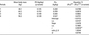
The pigs of Table 2 and equation (12) have a point of inflection P/α = 0.161 (Table 1). This is much lower than the values calculated for pigs by Knap (Reference Knap2000) from the Bridges equation. In contrast to equation (12), the growth data of Quiniou et al. (Reference Quiniou, Dourmad and Noblet1996; Table 5) indicate a point of inflection during their period 2, which cannot be reconciled with a value of P/α = 0.161. It therefore seems worthwhile to illustrate the fit of equation (7) on the data of Quiniou et al. (Reference Quiniou, Dourmad and Noblet1996) in Table 5.

Table 5

The fitting of equation (7) to average protein retention and protein maturity (P/α) in four growth periods on data published by Quiniou et al. (Reference Quiniou, Dourmad and Noblet1996)

Q, the ratio of the total experiment protein retention (PR) to the ad libitum average PR.

Roux (Reference Roux2005a) gives an example in which the fitting of power curves for the description of PB and PS gives estimates of limit or mature protein mass in agreement with the estimates from the fitting of Gompertz curves by Knap (Reference Knap2000). Knap’s (2000) collation of data from the literature contains that of Tullis (Reference Tullis1981) with some observations very near to maturity. The estimates obtained from Tullis (Reference Tullis1981) are well contained within the confines of the total collection of estimates. It seems, therefore, that the somewhat premature truncation of growth records in other cases did not cause any serious bias in Knap’s (Reference Knap2000) estimates of protein limit mass. However, Knap’s (Reference Knap2000) limit masses show clear sex differences with averages of α = 26.4 for castrates, α = 30.3 for females and α = 32.9 for males, with n = 3 for both males and castrates and n = 4 for females, on discarding an outlying male estimate of α = 38.5. Since estimates of protein limit mass show no time trend indicative of selection improvement, these estimates can be used when estimates for specific types or breeds are unavailable or not reliable.

As estimates of PR are subject to measurement error as well as individual variability and the differences are small in the body mass range under consideration, I fitted curves to averages over all sexes, breeds and nutritional treatments. One-third of the pigs were male and two-thirds were castrates, so that limit protein mass is estimated by α = 1/3 × 32.9 + 2/3 × 26.4 = 28.6 (Table 5). Protein mass is obtained by assuming it to be a fraction of 0.16 of live body mass (Agricultural Research Council (ARC), 1981). Table 5 shows that PR is maximum in period 2 with an approximate value of P/α = 0.359. Table 1 indicates consonance with X + Z = 10/9 for (4/9)Y = 2/9 for whole body protein. Hence, from equation (7), one would like to fit

(13)

This can be done by regression of PR on (P/α)^8/9−(P/α)^10/9 through the origin. To test for goodness of fit, an ordinary regression analysis was performed. The highly significant correlation coefficient of 0.9918 indicates excellent fit and the non-significant intercept indicates the acceptability of a fit through the origin. The slope through the origin is estimated by the ratio of the averages of the y and x regression variables and Q is the ratio of total experiment average PR to the ad libitum average PR. Analysis by Quiniou et al. (Reference Quiniou, Dourmad and Noblet1996) suggests that ad libitum PR is equivalent to PR_max in their data. It follows that c in equation (13) can be estimated by 1.8544/0.8746 = 2.1203. Accepting as in equation (12) a 3/4 power relationship with α, the constant c becomes c = 2.1203/(28.6)^3/4 = 0.1714α ^3/4. Hence, equation (13) becomes

(14)

Inclusion of the term α ^3/4 would allow for comparison with or prediction between species, breeds or types with different limit protein masses but the same powers for (P/α) in equations (7) or (14). Such a scaling of PR with protein limit mass is, furthermore, in agreement with Taylor’s (Reference Taylor1980) genetic scaling rules in animal growth. This matter will be further discussed in Roux (Reference Roux2010).

Body mass evidence

Fish body mass growth

Ursin (Reference Ursin1979) used equation (1) with body mass as a variate to describe fish body mass growth and estimated a and b together with 95% confidence limits from a detailed analysis of the growth curves of 81 fish species as

(15)

Since the fish’s empty body does not contain much fat, it is assumed that P ∝ W ^1.09 or W ∝ P ^0.92 like lean pigs (Siebrits, Reference Siebrits1984). Then dW/dt = P ^−0.08dP/dt, so that substitution of W with P ^0.92 in dW/dt = c ₄W ^0.59−c ₃W ^0.83 (equation 15) gives

(16)

with c ₁, c ₂, c ₃ and c ₄ as arbitrary constants. From equation (7), it follows that X + Z = 0.84 and X + Z−(4/9)Y = 0.62. Solving for Y gives Y = 1/2, or (4/9)Y = 2/9, in agreement with the mammalian estimates. According to Fauconneau and Arnal (Reference Fauconneau and Arnal1985), muscle provides a fraction of 0.22 of PS in Rainbow trout, near enough to the 0.25 fraction assumed in Roux (Reference Roux2006) for the derivation of Y = 1/2 for total body protein in mammals. Hence, equations (15) and (16) are in agreement with the theory encompassed in equation (7).

Variation in body mass growth form

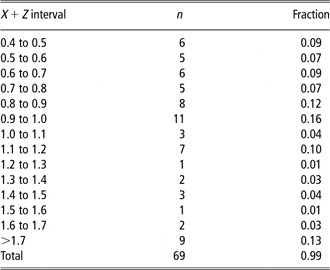
Variation in body mass growth form has been investigated by Gaillard et al. (Reference Gaillard, Pontier, Allaine, Loison, Herve and Heizmann1997) by fitting the Richards (Reference Richards1959) growth curve family from birth to adulthood to 69 species of eutherian mammals. They showed that growth form differs significantly among eutherian mammals and concluded that ‘the commonly used Gompertz model can no longer be considered as the general model for the description of mammalian growth.’ For each species, the inflection point was calculated according to von Bertalanffy (Reference von Bertalanffy1960). From the inflection points, values of X + Z were calculated from equation (9) and are given in Table 6, on the supposition of a fit by equation (7) with Y = 1/2 on the assumption of whole body P ∝ W.

Table 6

The distribution of values of the powers of protein breakdown rate X + Z estimated from the inflection points of the family of curves fitted to mammalian body mass growth data by Gaillard et al. (Reference Gaillard, Pontier, Allaine, Loison, Herve and Heizmann1997)

Inflection points before birth can only be accurately estimated from prenatal observations. Hence, inaccurate or unrealistic negative estimates were replaced by the best available approximate estimates of (birth mass)/(adult body mass) for the estimation of X + Z in Table 6. This creates consonance between the lowest values in Table 6 and those in Table 1.

Judged by the significance of the Richards shape parameter (Gaillard et al., Reference Gaillard, Pontier, Allaine, Loison, Herve and Heizmann1997), only two estimates of X + Z larger than 1.7 in Table 6 are significantly larger than the maximum value of Table 1 in line 12 at the 0.05 level and none at the 0.01 level. For a sample of 69, this is about what one would expect to occur by chance, from the definition of a type 1 error. In addition, seven of the nine outliers larger than 1.7 are rodents, either squirrels or chipmunks, known as hibernators to build up body fat to survive the winter asleep. This possibly fast increase in body fat near maturity may explain a late point of inflection in body mass, not necessarily approximately coinciding with a point of inflection in protein mass. Hence, without further evidence on whole body protein growth, the outliers in Table 6 cannot be regarded as evidence of a possible inadequacy of Table 1 in the explanation of whole body protein growth.

It is clear from equation (7) that variable values of Q will distort the observed growth pattern. The relationship of Q to nutrition is given by equation (10). Presumably, animals are customarily fed to the ad libitum level in growth studies. Since PR_max is achievable in pigs (Moughan, Reference Moughan1999), ad libitum intake on nutritious food could generally result in Q = 1. Hence, the assumption of approximate constancy of Q during growth from birth to maturity may be realistic for many of the growth curves of Gaillard et al. (Reference Gaillard, Pontier, Allaine, Loison, Herve and Heizmann1997). Overall, the evidence in Table 6 may therefore indicate that most species have X + Z values according to lines 1 to 6 in Table 1, but that a significant minority has to be accommodated by lines 7 to 12. This is in agreement with the evidence in Tables 2 to 4.

The significant differences in body protein X + Z powers obtained in Tables 3 and 4 also argue against the possibility that the significantly different body mass fit of different members of the Richards family is solely due to nutrition, body composition or other environmental effects, masking the only true mammalian body protein growth curve. The alternative to a single growth curve is a family or distribution of growth curves based on Table 1. The distribution in Table 6 suggests either X + Z = 8/9 or slightly less likely X + Z = 1, from Table 1, as the median or modal values of such a distribution.

Growth of other chemical components and intake prediction

By assuming power relationships between body protein and other chemical components, appropriate growth curves for these chemical components can be derived. This is illustrated for fat growth in Roux (Reference Roux2010), together with applications of protein and fat growth descriptions in intake prediction.