Relationships between productivity and production costs

Production is a technical process, analytically described using a production function, which relates certain factors (e.g. energy, raw materials, working hours etc.) with total production output. Analytically these relationships are presented by either technical coefficients or their reverse values, i.e. average productivity (equations 1 and 2):

(1)

This ‘average productivity’ measures the amount of total product per unit of i-th production factor X. If we multiply the amount of the i-th production factor used by the relevant price of the factor the costs of the i-th production factor can be established. When combining these partial costs, it is possible to obtain total production costs according to the following equation 3:

(2)

Finally, if the total costs are divided by the amount of production, the average costs can be calculated thus (Equation 4):

(3)

Relating average productivity with average costs and keeping the price of each production factor used constant, an inverse relationship between average productivity and average costs is obtained, whereby an increase of AP_x resulted in growth of TP by keeping the amount of production factor used unchanged. Due to the application of constant prices of production factors and where the production factor remains unchanged, the numerator is unchanged and the denominator is higher, thus causing a decrease of the AC, and vice versa.

If we introduce average productivity - average costs (AP_X - AC) into this relationship, as an optimal criteria, relationships between technical and cost efficiencies can be established. Such optimal criterions include the following:

• • In the case of average productivity, the optimality criterion should be the highest possible amount of production per i-th production factor used.

• • In the case of average costs this criterion should be the lowest possible cost per unit of product.

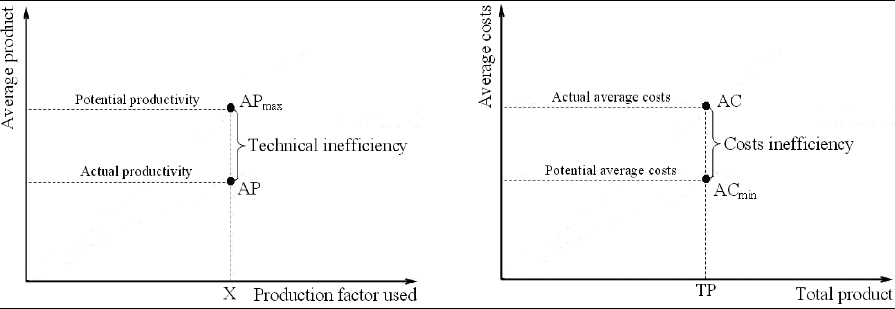
Figure 1 describes the technical and cost inefficiency relationship, and is composed of two parts. On the left side, the graphical deduction of technical inefficiency is presented, where the amount of production factor used equals X and is related with the average productivity at the AP level. Actual productivity level is below potential productivity (AP _max). The observed distance between actual and potential productivity is termed as ‘technical inefficiency’. On the right side of Figure 1 the cost inefficiency is represented, where the amount of production equals TP and is related with the average cost at the AC level. Actual average cost level is above the potentially lowest level (AC _min). The observed distance between actual and potential average cost is termed as ‘cost inefficiency’.

Figure 1

Technical and cost inefficiency.

Source: Novak and Žižmond (Reference NOVAK and ŽIŽMOND2012).

Novak and Žižmond (Reference NOVAK and ŽIŽMOND2012) utilised two different terms with equal meaning: technical inefficiency and efficiency, where both measured the difference between actual and potential productivity, as well as cost inefficiency and efficiency, which measured the difference between actual and potential average costs. In their deduction of the OCE algorithm they introduced technical efficiency and cost inefficiency rates (TER and CIR). Technical efficiency rate was defined as the ratio between actual and potential productivity, where cost inefficiency rate was the ratio between actual and potential average costs (Novak and Žižmond, Reference NOVAK and ŽIŽMOND2012; equations 5 and 6):

(4)

If AP equals AP _max then TER equals 1, implying that full technical efficiency minus the actual amount of production equals the potential amount of production. If AC equals AC _min, then CIR equals one, implying zero cost inefficiency (or full costs efficiency) which can only be achieved in the case of full technical efficiency. According to such calculations, inverse relationships exist between technical efficiency and cost inefficiency. If technical efficiency rises towards one, cost inefficiency decreases towards one, and if technical efficiency decreases towards zero, cost inefficiency increases towards infinity.

Overall equipment and cost efficiencies

In manufacturing practice, especially in the case of automated production lines for mass production of pate, the use of a key performance indicator (KPI) termed as OEE is applied. The OEE was introduced by Nakajima (Reference NAKAJIMA1998), and was aimed at supporting the processes of total productivity maintenance (TPM). OEE is a productivity measure that estimates technical efficiency by controlling the availability, performance and quality of the production process (Huang et al., Reference HUANG, DISMUKES, SHI, SU, RAZZAK, BODHALE and ROBINSON2003; De Ron and Rooda, Reference DE RON and ROODA2006; Jonsson and Lesshammar, Reference JONSSON and LESSHAMMAR1999). There exist different varieties of the mathematical specification of an OEE, where the common framework is given as (Novak and Žižmond, Reference NOVAK and ŽIŽMOND2012; equation 7).

(5)

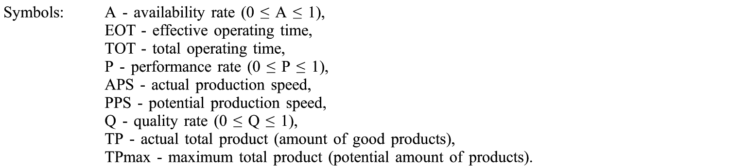
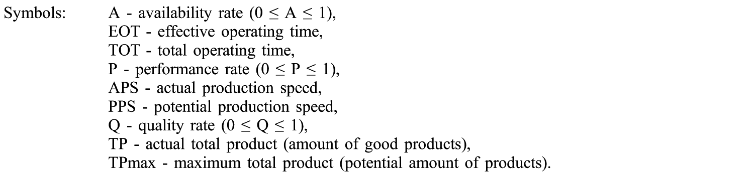
There are three parameters of OEE. The first parameter is availability rate (A) which measures the share of effective versus total operating time. The total operating time (TOT) is a time-span within which the production process can proceed. However, due to varying reasons including cleaning or repair, the production process does not take place within the TOT. Therefore, a time when the production process is in full capacity use is measured as the effective operating time (EOT). The second parameter is performance rate (P), which is a relative coefficient with an actual production speed (APS) in the numerator and a potential production speed (PPS) in the denominator. This measures the amount of production in a certain unit of time (e.g. 1000 pieces per hour). The third parameter is quality (Q), which measures the amount of good pieces made within the total production and realized within the EOT and at a given performance of the production line. The following definition equation is used for each partial parameter of OEE (Novak and Žižmond, Reference NOVAK and ŽIŽMOND2012; equations 8, 9 and 10):

(6)

In the case of full availability, performance and quality of production, there is no deviation between the actual and potential product. However, due to various inefficiencies, the actual amount of production is reduced below its potential level, and the OEE diminishes towards its minimum level zero.

The term OCE (Novak and Žižmond, Reference NOVAK and ŽIŽMOND2012) was proposed as this parameter is deduced from OEE. These authors developed the OCE parameter by introducing the OEE coefficient into the CIR definition equation (6) and applied microeconomic equality, where total cost (TC) consisted of fixed costs (FC) and variable costs (VC), or, when total cost was divided by total product (TP), it held that average cost (AC) consisted of average fixed cost (AFC) and average variable cost (AVC). They then performed an eight-step procedure to reach a final definitive equation for OCE (equation 11):

(7)

As seen from equation (11), there was an inverse relationship between OCE and OEE, where quality rate had an additional impact via variable costs. The equation can be used to mathematically deduce an estimator that transforms technical efficiency into cost inefficiency. There are four factors that determine the impact of technical efficiency on cost inefficiency (Novak and Žižmond, Reference NOVAK and ŽIŽMOND2012):

• • The first impact is controlled by the inverse value of OEE (0≤OEE≤1). Therefore, if OEE diminishes towards zero, its inverse value rises towards infinity, and if it rises towards one, its inverse value diminishes towards one.

• • The second impact is controlled via the proportion of fixed costs within total costs. The domain of this ratio is [0, 1] and is zero where total costs are variable, and one if they are fixed. The greater the share of fixed costs versus total costs, the higher the impact of technical efficiency on cost inefficiency.

• • The third impact is controlled via the inverse value of quality. The domain of the inverse ratio is between [1,). It is 1 in the case of full quality, while decreasing quality rate causes its growth towards.

• • The fourth factor is controlled via the share of average variable costs within average costs. The domain of this share is between [0, 1], i.e. it is zero if total costs are fixed, and one if variable.

Poultry pâté production process

Equation 11 is a suitable application for any automated industry, including poultry pate production. According to the proposed algorithm, only data on the proportion of fixed and variable costs within average costs are needed.

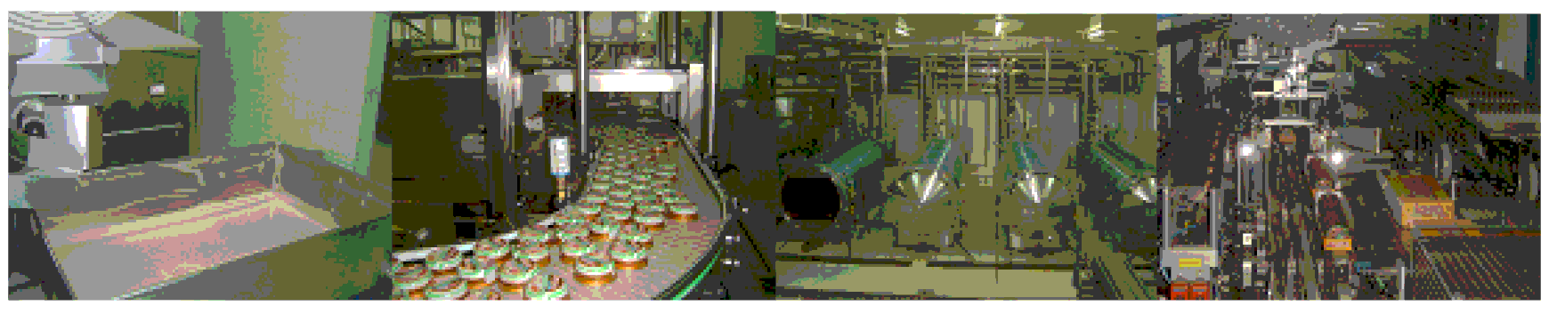
Automated lines for poultry pâté production (Figure 2) are organised as an integrated system of four key production processes: preparation and cooking the meat, adding extra ingredients to the pate, filling individual servings, sterilisation and final packaging.

All production phases represent a comprehensive process, i.e. all are required for final product.

Figure 2

Poultry pâté production process

Measurements on technical efficiency of pâté production

From the viewpoint of technical efficiency, all production phases should be efficient, as the main aim is to ensure uninterrupted production. From the cost efficiency point of view the crucial phase is the packaging of containers, and so analysis is focussed on measuring technical efficiency on the process of packaging.

Real time measurements of OEE were performed on a daily basis, giving the unit of observation as one day for the separate parameters of OEE, according to equations 7-10, with a total of 150 observations (days).

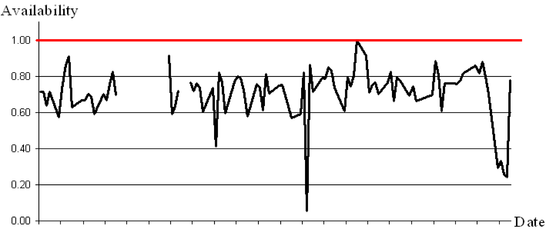
The first parameter measured was availability (A) of the production (i.e. packaging) line. According to equation 8, this measures the ratio between the effective and total operating time. In this case the daily working time was 16 hours (two shifts), the total operating time was the daily working time less planned interruptions. As planned interruptions amounted to 2.4 hours per day, the total operating time is 16 - 2.4 = 13.6 hours per day, which was set as a constant. The EOT was the total operating time less unplanned interruptions (Figure 3).

Figure 3

Availability rate of the packaging line (potential available time = 13.6 hours).

Source: own observations and measurements.

Number of observations: n = 150.

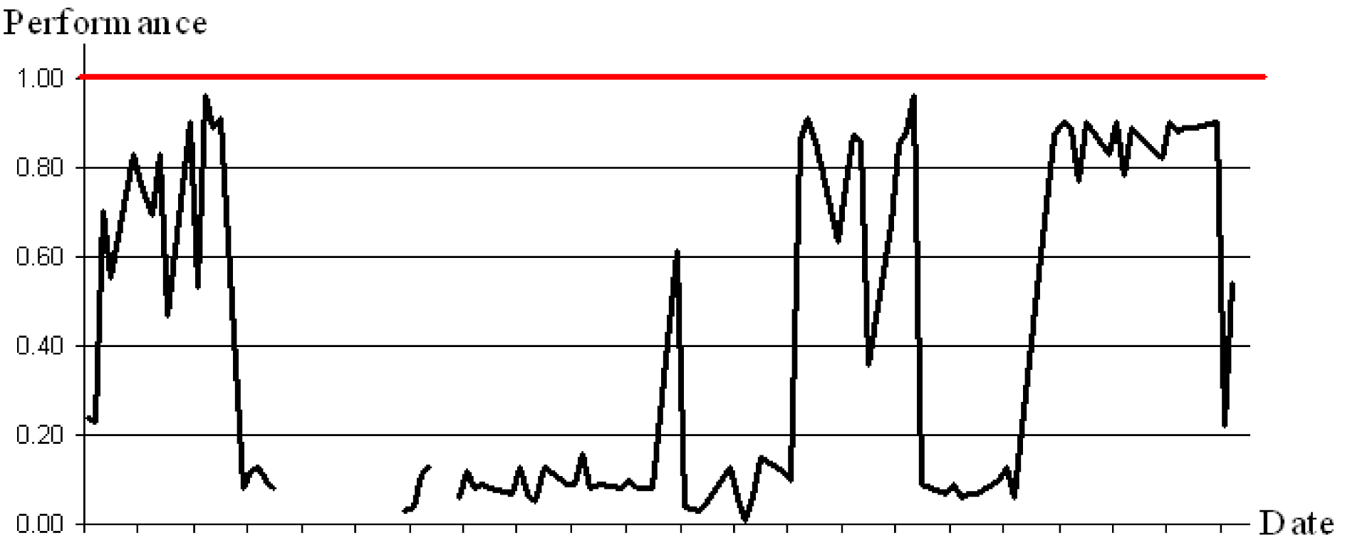
From the 150 measurements it was concluded that the availability rate of the production line of packaging amounted to, on average, 71.23 %. The P according to equation 9, was a relative coefficient with an APS in the numerator and a PPS in the denominator. The performance was measured within the time frame of actual availability of the production line (Figure 4).

Figure 4

Performance rate of the packaging line (according to actual available time).

Source: own observations and measurements.

Number of observations: n = 150.

From the 150 measurements it was concluded that the average value of P was 39.23 %. This means that on average the actual speed of the production line was almost 60% lower than its potential speed within the actual available time of the production line.

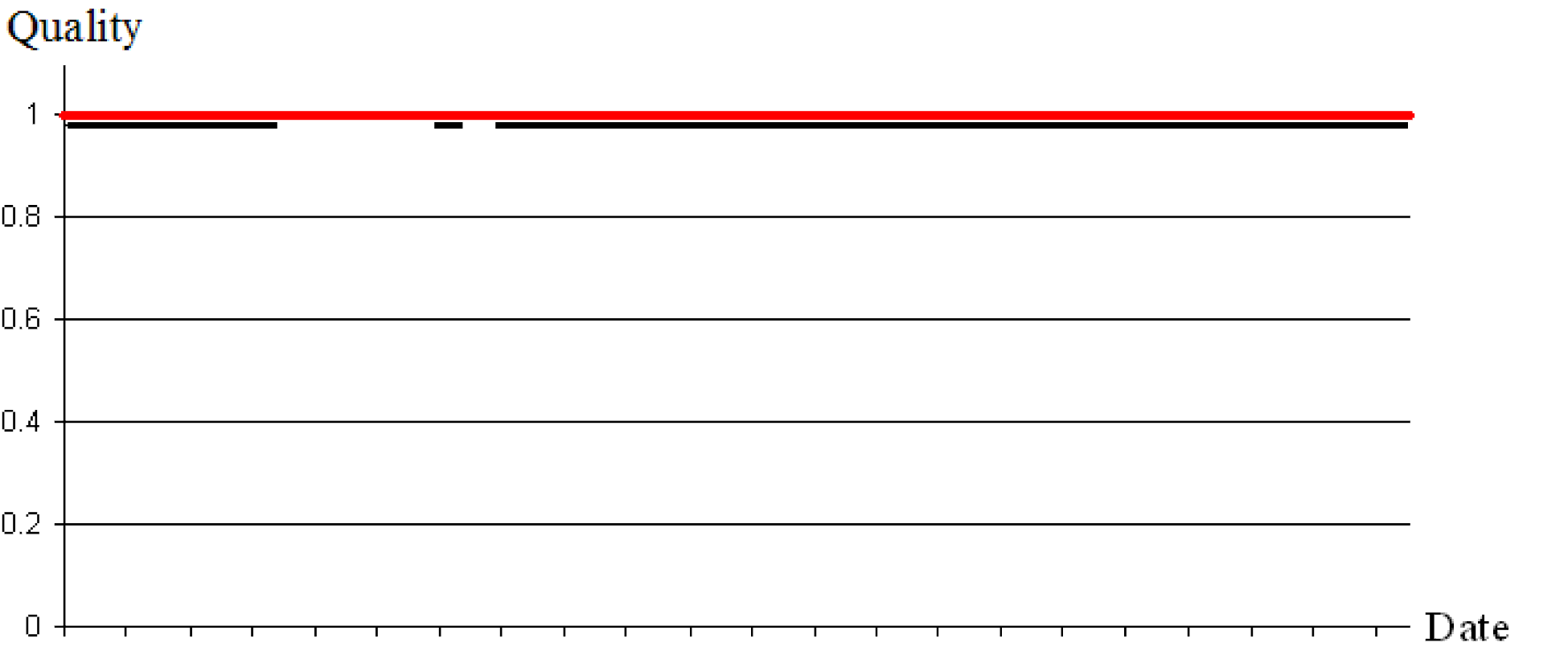
Quality is final parameter, and, according to equation 10, is defined as a share of good pieces of production in the total production realised within the effective operating time and at the given performance of the production line (Figure 5).

Figure 5

Quality rate for the observed production process.

Source: own observations and measurements.

Number of observations: n = 150.

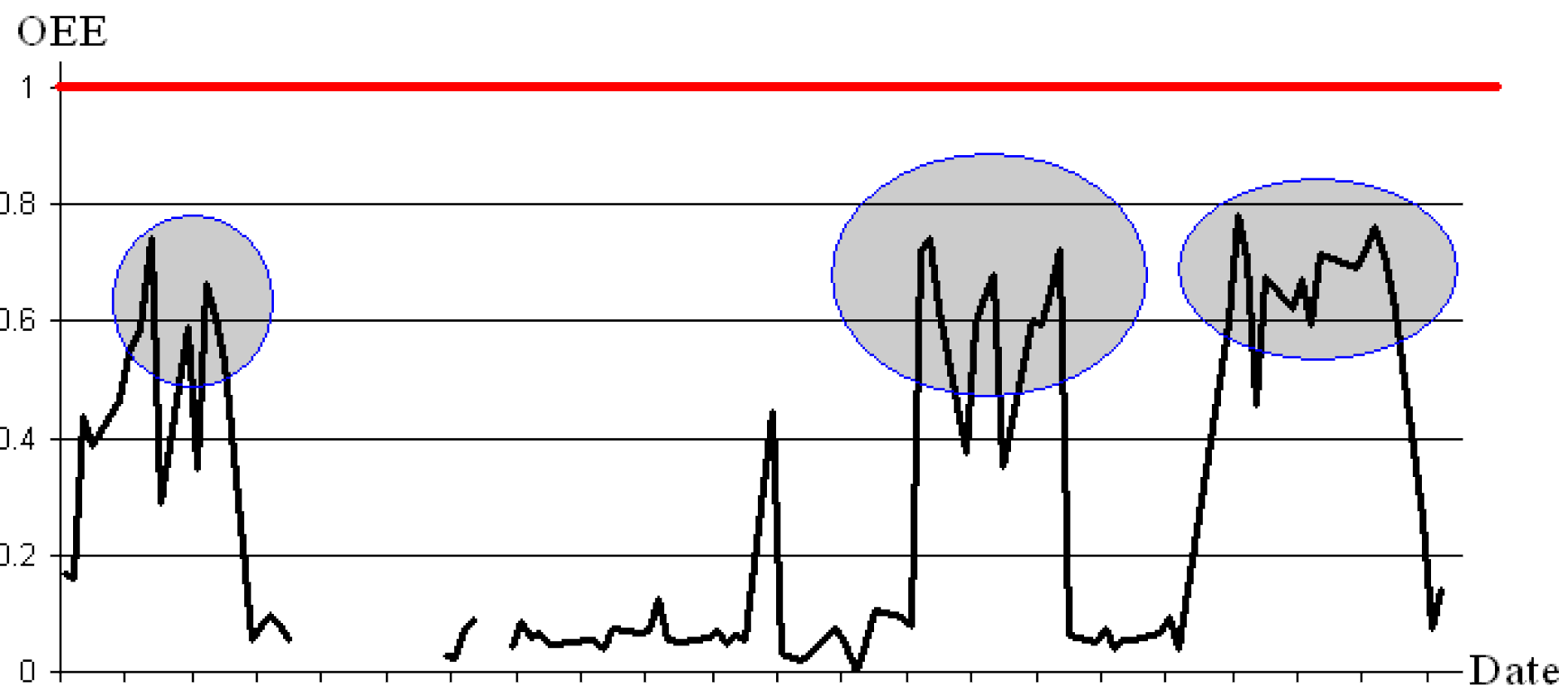
Following these observations, quality rate remained constant over time at a level of 98% on the basis of partial real time measurement of all production parameters (availability, performance and quality). The OEE measured the level of technical efficiency within the interval [0, 1]. Increasing OEE towards 1 means increasing (improving) of technical efficiency, and vice versa. In our case the average value of parameter OEE was 0.2915. This meant the actual quantity of production reached, on average, a little less than 30% of the potential amount of production in the observed period (Figure 6).

Figure 6

Values of parameter OEE for the packaging line of great pâtés.

Source: own observations and measurements.

Number of observations: n = 150.

Very low average values for OEE was seen in summer periods of production. When summer observations of OEE and some extreme daily falls in OEE were removed the average value of OEE was 0.6861. This means that the actual quantity of production reached a little less than 70% of the potential amount of production.

OCE - empirical analysis of costs efficiency

As we know from equation 11, all daily calculated OEE values can be translated into OCE which can be used to determine if the APC of poultry pâté is more expensive, as it will be in the case of full technical efficiency.

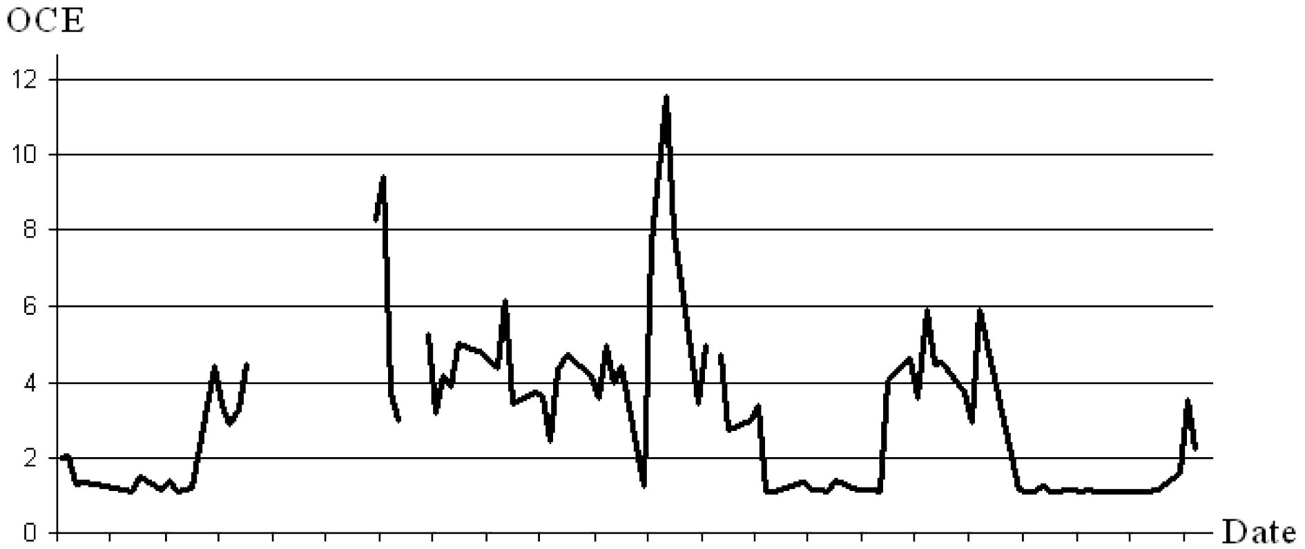
As we know from equation 11, when estimating the cost efficiency the essential point is establishing the proportion of fixed and variable costs within total costs. In the case of pate production, the average relationship between costs is 20% fixed costs and 80% variable costs. This ratio was used as a standard in our estimations of cost efficiency (Figure 7).

Figure 7

Estimations of cost efficiency (OCE) of packaging line of poultry pâtés.

Source: own observations and measurements.

Number of observations: n = 150.

From the obtained OCE calculations for 150 days, it was seen that the average value of pate OCE was 2.99. This implied that actual average costs exceeded the potential minimum average costs by almost three times. One produced package of poultry pâté is therefore around 200% more expensive than it could be if the line was working at full technical efficiency.

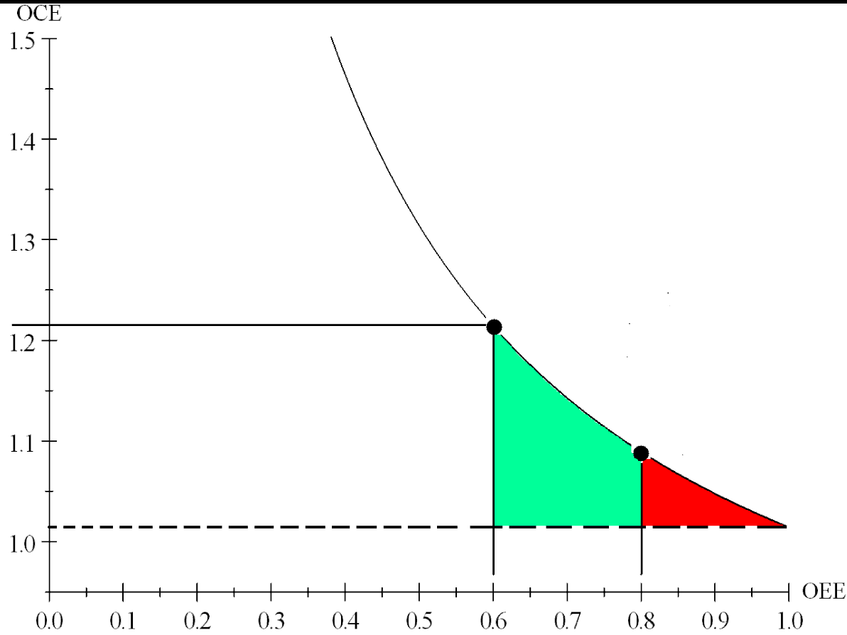
By using average values of OCE and OEE, it is possible to relate OCE with OEE, where OEE is the explanatory variable and OCE is the dependant variable.

Figure 8 shows the mathematical equation which translated OEE into OCE and which can be used as efficient analytical tool for production management. It demonstrated how much cost efficiency can improve with increasing technical efficiency. In the case of pate production, the increase in technical efficiency from 60% to 80 % of potential production decreases cost inefficiency from 1.21 to 1.10.

Figure 8

OEE - OCE relationship.

Source: own calculations and measurements.

The causal relationship between OEE and OCE demonstrated the value added by using OCE methodology, when it is successfully implemented into the industrial management praxis. As demonstrated, it is possible to achieve large improvements in technical efficiency but this will result in only a small reduction in cost inefficiency. Therefore an efficient and successful industrial management needs to utilise both the OEE framework with the proposed OCE methodology.