1 Introduction
General features of planetary atmospheres such as alternating bands and currents, exemplified by the jet streams on Earth and more prominently on Jupiter and the giant gas planets, are known to be strongly affected by planetary rotation, specifically the latitudinal variation in planetary potential vorticity (PV). Nowhere else is this better seen than on Jupiter, a rapidly rotating planet with a particularly active atmosphere (Rogers Reference Rogers1995). Observations of Jupiter in fact go back to ancient times. Babylonian astronomers first recorded the appearance of the planet (Sachs Reference Sachs1974), and for them it was a bright star in the celestial sky. In 1630 with the improvement of optics, Jupiter’s bands were first captured by Niccolo Zucchi. Then, Hooke and Cassini in 1664 and 1665 detected spots, now known as vortices (Rogers Reference Rogers1995). Hence, the presence of bands and vortices was already known at this time. Much more recently, spacecraft observations have revealed complex turbulent dynamics occurring in Jupiter’s atmosphere, composed of quasi-zonal jets and myriads of vortices like the Great Red Spot (see Dowling & Ingersoll Reference Dowling and Ingersoll1988; Marcus Reference Marcus1993).
The outer Jovian atmosphere is structured in zonal bands, called belts and zones. They are separated by jets which are strong currents flowing eastwards around the planet. Contrary to Earth’s jets, Jovian jets are remarkably straight, with few large-scale meanders. Hubble offers us a visualisation of the Jovian atmosphere’s external layer where jets and vortices are clearly present (see Simon, Wong & Orton (Reference Simon, Wong and Orton2015) and for previous observations see Limaye (Reference Limaye1986) and Porco et al. (Reference Porco, West, McEwen, Del Genio, Ingersoll, Thomas, Squyres, Dones, Murray and Johnson2003)). (Movie available at http://svs.gsfc.nasa.gov/cgi-bin/details.cgi?aid=12021.) Observations of Jupiter have in turn inspired researchers to develop idealised models of the Jovian atmosphere (see e.g. Dowling Reference Dowling1995; Ingersoll et al. Reference Ingersoll, Dowling, Gierasch, Orton, Read, Sanchez-Lavega, Showman, Simon-Miller and Vasavada2004).
Such models generally differ as regards the vertical structure of the Jovian atmosphere. Actual data are sparse: we have only a single vertical profile collected by the Galileo probe (see Atkinson, Pollack & Seiff Reference Atkinson, Pollack and Seiff1998), which cannot be argued to be representative. To gain at least a qualitative understanding of the dynamics of Jupiter and of the gas giants generally, two main modelling approaches have been taken: a shallow model and a deep model. The shallow model (typically employing the rotating shallow-water equations in a single layer) suggests that jets emerge essentially through an upscale cascade of geostrophic turbulence (Williams Reference Williams1978; Cho & Polvani Reference Cho and Polvani1996; Kaspi & Flierl Reference Kaspi and Flierl2007; Scott Reference Scott2007; Showman Reference Showman2007). By contrast, the deep model suggests that the flow is organised in deep concentric rotating cylinders, with jets their external representation, (see Busse Reference Busse1970, Reference Busse1976). Kaspi, Flierl & Showman (Reference Kaspi, Flierl and Showman2009) studied a three-dimensional non-hydrostatic general circulation model, with a large density variation under the anelastic approximation. Unlike in models employing the Boussinesq approximation valid for weak density variations, they observe the development of baroclinic shear (a strong increase of horizontal wind speed with height). Likewise, Liu & Schneider (Reference Liu and Schneider2010) and Spiga et al. (Reference Spiga, Guerlet, Meurdesoif, Indurain, Millour, Dubos, Sylvestre, Leconte and Fouchet2015) used general circulation models to study the atmospheres of the gas giants. Liu & Schneider (Reference Liu and Schneider2010) were able to reproduce main features of the large-scale circulation on both Jupiter and Saturn, and found that zonal jets extend down to a depth where drag is assumed to become important. Spiga et al. (Reference Spiga, Guerlet, Meurdesoif, Indurain, Millour, Dubos, Sylvestre, Leconte and Fouchet2015) focused on Saturn and included specifically the roles of aerosol layers, ring shadowing and internal heat fluxes. They found that zonal jets develop in the troposphere and equatorial oscillations occur in the stratosphere. In summary, it has been argued that many models, having widely different formulations, capture qualitative features of planetary circulations on the gas giants.
On Earth, both the atmosphere and the oceans exhibit similar dynamical structures. The jets occurring in the oceans, however, are typically strongly meandering and unsteady (see Maximenko, Bang & Sasaki Reference Maximenko, Bang and Sasaki2005; Kamenkovich, Berloff & Pedlosky Reference Kamenkovich, Berloff and Pedlosky2009; Berloff et al. Reference Berloff, Karabasov, Farrar and Kamenkovich2011). The most well-known oceanic jets are the strong oceanic currents like the Gulf Stream and the Kuroshio. The jets occurring in the atmosphere also exhibit large-scale meanders but are generally much more well defined than their oceanic counterparts.
Arbic & Flierl (Reference Arbic and Flierl2004) and Thompson & Young (Reference Thompson and Young2007) studied the impact of bottom friction on oceanic simulations. Arbic & Flierl (Reference Arbic and Flierl2004) examined the energetics behind the formation of mid-ocean eddies, while Thompson & Young (Reference Thompson and Young2007) focused on the role of the baroclinic (vertically varying) mode on the eddy heat flux. Venaille, Nadeau & Vallis (Reference Venaille, Nadeau and Vallis2014), using a two-layer quasi-geostrophic model on the
 $f$
-plane (uniform background rotation) found that for a small bottom friction the flow forms approximately barotropic (height independent) large-scale structures, which persist over a time scale inversely proportional to the bottom friction damping rate. However, for high bottom friction, the upper layer flow dominates at leading order in the inverse damping rate. In this case, the upper flow behaves like a single-layer shallow-water flow (a
 $1\frac{1}{2}$
-layer model) and exhibits coherent jets separating regions of nearly homogeneous PV.
To develop a conceptual understanding of Jovian jets and vortices, Thomson & McIntyre (Reference Thomson and Mcintyre2016) recently proposed a
 $1\frac{1}{2}$
-layer quasi-geostrophic model based on the Dowling and Ingersoll model (see Dowling & Ingersoll Reference Dowling and Ingersoll1989), with predefined jets (created by an imposed lower boundary shape interface) and forced by the injection of cyclone/anti-cyclone pairs. With this idealised Jovian weather-like model, they managed to reproduce observed features such as nearly steady and straight (zonal) jets together with long-lived vortices.
The goal of the present study is to better understand the vertical structure of jets and vortices in a turbulent planetary atmosphere. A two-layer quasi-geostrophic shallow-water
 $\unicode[STIX]{x1D6FD}$
-channel model is used to examine the formation and evolution of jets and vortices, and in particular their sensitivity to vertical shear, forcing and damping. Following Panetta & Held (Reference Panetta and Held1988), a vertical shear is imposed by relaxing to a thermal equilibrium temperature gradient – however we do not include Ekman damping or any bottom friction (see Venaille et al. (Reference Venaille, Nadeau and Vallis2014) for the impact of bottom friction on a two-layer quasi-geostrophic model). Bottom friction is not relevant in shallow models of the gas giants (Thomson & McIntyre Reference Thomson and Mcintyre2016). The vertical shear induces baroclinic instability, whose nonlinear equilibration attempts to reduce the shear. This competition between thermal forcing and baroclinic instability gives rise to the formation of baroclinic jets and, in extreme cases, to stepped PV profiles or ‘staircases’. Such staircase formation has already been demonstrated in the single-layer barotropic context (see Dritschel & McIntyre Reference Dritschel and Mcintyre2008; Scott & Dritschel Reference Scott and Dritschel2012). Additionally, in the present model small-scale stochastic forcing is imposed, crudely mimicking convective processes. This is done by adding hetons or small cyclonic/anti-cyclonic pairs in the two layers. Unlike in the model of Thomson & McIntyre (Reference Thomson and Mcintyre2016), jets do not emerge from an imposed lower boundary shape but emerge naturally from the competition between baroclinic instability and thermal damping.
Section 2 presents the model, the equations and the boundary conditions. Section 3 presents the results, starting with an analysis of a characteristic simulation, followed by a detailed examination of energy transfers in § 4. We then focus on a turbulent event in § 5 and discuss the wider parameter dependence in § 6. Finally, § 7 presents our conclusions and a few ideas for future research.
2 Model formulation
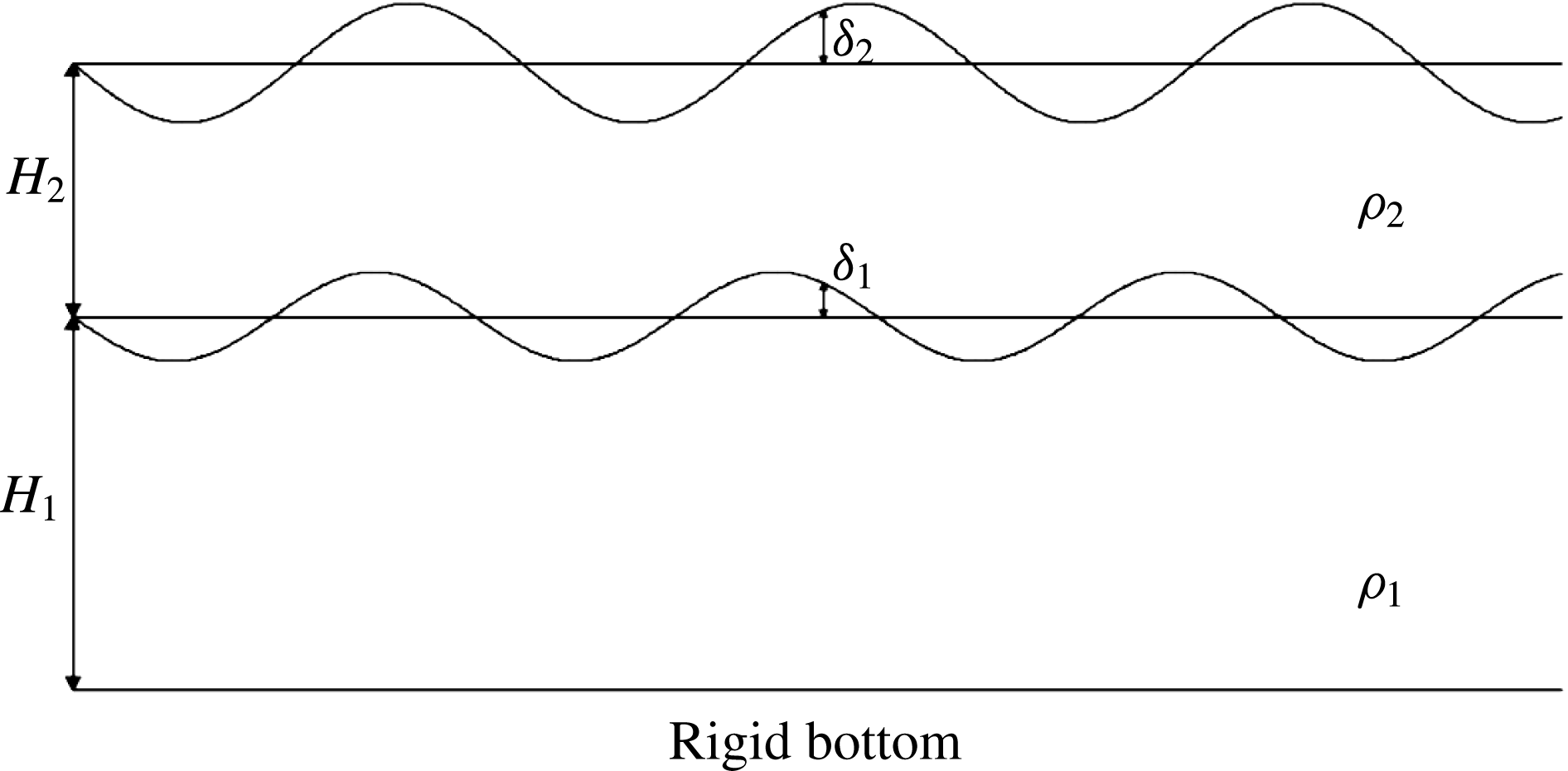
Vertical cross-section of the model. Here,
 $H_{1}$
and
 $H_{2}$
are the mean layer thicknesses,
 $\unicode[STIX]{x1D70C}_{1}$
and
 $\unicode[STIX]{x1D70C}_{2}$
the layer densities and
 $\unicode[STIX]{x1D6FF}_{1}$
and
 $\unicode[STIX]{x1D6FF}_{2}$
the displacements of the middle and upper interfaces.

To study the formation and evolution of jets and vortices in turbulent planetary atmospheres, we make use of a two-layer quasi-geostrophic (QG)
 $\unicode[STIX]{x1D6FD}$
-channel model (see Phillips Reference Phillips1951), with a rigid bottom and a free upper surface (see figure 1). It is governed by the set of equations:
 $$\begin{eqnarray}\displaystyle \frac{\text{D}q_{1}}{\text{D}t}=F_{1};\quad \frac{\text{D}q_{2}}{\text{D}t}=F_{2}, & & \displaystyle\end{eqnarray}$$
 $$\begin{eqnarray}\displaystyle q_{1}=\unicode[STIX]{x1D6FD}y+\unicode[STIX]{x1D6FB}^{2}\unicode[STIX]{x1D713}_{1}-\frac{f_{0}\unicode[STIX]{x1D6FF}_{1}}{H_{1}};\quad q_{2}=\unicode[STIX]{x1D6FD}y+\unicode[STIX]{x1D6FB}^{2}\unicode[STIX]{x1D713}_{2}-\frac{f_{0}(\unicode[STIX]{x1D6FF}_{2}-\unicode[STIX]{x1D6FF}_{1})}{H_{2}}, & & \displaystyle\end{eqnarray}$$
 $$\begin{eqnarray}\displaystyle \unicode[STIX]{x1D6FF}_{1}=\frac{f_{0}(\unicode[STIX]{x1D713}_{1}-\unicode[STIX]{x1D6FC}\unicode[STIX]{x1D713}_{2})}{g(1-\unicode[STIX]{x1D6FC})};\quad \unicode[STIX]{x1D6FF}_{2}=\frac{f_{0}\unicode[STIX]{x1D713}_{2}}{g}, & & \displaystyle\end{eqnarray}$$
where
 $\text{D}/\text{D}t=\unicode[STIX]{x2202}/\unicode[STIX]{x2202}t+\boldsymbol{u}\boldsymbol{\cdot }\unicode[STIX]{x1D735}$
is the material derivative,
 $q_{i}$
is the quasi-geostrophic potential vorticity (QGPV) in layer
 $i$
,
 $F_{i}$
includes all forcing and damping on the QGPV in layer
 $i$
,
 $\unicode[STIX]{x1D6FD}$
is the linear gradient of the Coriolis frequency
 $f=f_{0}+\unicode[STIX]{x1D6FD}y$
,
 $\unicode[STIX]{x1D713}_{i}$
is the streamfunction in layer
 $i$
,
 $\unicode[STIX]{x1D6FF}_{i}$
is the displacement of the upper interface of layer
 $i$
,
 $H_{i}$
is the mean depth of layer
 $i$
,
 $\unicode[STIX]{x1D70C}_{i}$
the uniform density in layer
 $i$
,
 $\unicode[STIX]{x1D6FC}=\unicode[STIX]{x1D70C}_{2}/\unicode[STIX]{x1D70C}_{1}$
is the density ratio and
 $g$
is the acceleration due to gravity. We eliminate all reference to
 $f_{0}$
,
 $g$
and the total mean depth
 $H=H_{1}+H_{2}$
by specifying the mean baroclinic Rossby deformation wavenumber,
 $\bar{k}_{d}$
, defined through
 $$\begin{eqnarray}\bar{k}_{d}^{2}=\frac{1}{L_{d}^{2}}=\frac{f_{0}^{2}H}{g(1-\unicode[STIX]{x1D6FC})H_{1}H_{2}}\end{eqnarray}$$
and making use of the fractional mean layer depths
 $h_{i}=H_{i}/H$
whose sum is unity (
 $h_{1}+h_{2}=1$
). Then the only explicit parameters are
 $h_{1}$
,
 $\bar{k}_{d}$
,
 $\unicode[STIX]{x1D6FC}$
and
 $\unicode[STIX]{x1D6FD}$
.
As explained e.g. in Vallis (Reference Vallis2006), the QGPV expressions in (2.1) derive from a series expansion of the shallow-water Rossby–Ertel PV,
 $q_{i}=(\unicode[STIX]{x1D701}_{i}+f)/(h_{i}(1+\tilde{h}_{i}))$
, where
 $\unicode[STIX]{x1D701}_{i}$
is the relative vorticity in layer
 $i$
and
 $\tilde{h}_{i}$
is the fractional layer depth perturbation defined by
 $\tilde{h}_{i}=(\unicode[STIX]{x1D6FF}_{i}-\unicode[STIX]{x1D6FF}_{i-1})/H_{i}$
, with
 $\unicode[STIX]{x1D6FF}_{0}=0$
. The leading-order non-constant terms, for
 $\unicode[STIX]{x1D701}_{i}/f\ll 1$
and
 $\tilde{h}_{i}\ll 1$
, define the QGPV:
 $$\begin{eqnarray}q_{i}=\unicode[STIX]{x1D6FD}y+\unicode[STIX]{x1D701}_{i}-f_{0}\tilde{h}_{i}.\end{eqnarray}$$
The interface displacements
 $\unicode[STIX]{x1D6FF}_{i}$
are related to the layer pressure perturbations
 $p_{i}$
through hydrostatic balance (cf. Mohebalhojeh & Dritschel Reference Mohebalhojeh and Dritschel2004):
 $$\begin{eqnarray}p_{i}=g\mathop{\sum }_{j=i}^{n}(\unicode[STIX]{x1D70C}_{j}-\unicode[STIX]{x1D70C}_{j+1})\unicode[STIX]{x1D6FF}_{j},\end{eqnarray}$$
where here
 $n=2$
and
 $\unicode[STIX]{x1D70C}_{n+1}=0$
. From geostrophic balance, we have
 $$\begin{eqnarray}p_{i}=\unicode[STIX]{x1D713}_{i}f_{0}\unicode[STIX]{x1D70C}_{i}\end{eqnarray}$$
together with
 $u_{i}=-\unicode[STIX]{x2202}\unicode[STIX]{x1D713}_{i}/\unicode[STIX]{x2202}y$
and
 $v_{i}=\unicode[STIX]{x2202}\unicode[STIX]{x1D713}_{i}/\unicode[STIX]{x2202}x$
. Using (2.6) and (2.7), we can re-express (2.5) for each layer as
 $$\begin{eqnarray}q_{1}=\unicode[STIX]{x1D6FD}y+\unicode[STIX]{x1D6FB}^{2}\unicode[STIX]{x1D713}_{1}+h_{2}\bar{k}_{d}^{2}(\unicode[STIX]{x1D6FC}\unicode[STIX]{x1D713}_{2}-\unicode[STIX]{x1D713}_{1});\quad q_{2}=\unicode[STIX]{x1D6FD}y+\unicode[STIX]{x1D6FB}^{2}\unicode[STIX]{x1D713}_{2}+h_{1}\bar{k}_{d}^{2}(\unicode[STIX]{x1D713}_{1}-\unicode[STIX]{x1D713}_{2}).\end{eqnarray}$$
These may be regarded as ‘inversion relations’ providing the flow field
 $\boldsymbol{u}_{i}$
in each layer (via
 $\unicode[STIX]{x1D713}_{i}$
) from the instantaneous distribution of QGPV (
 $q_{1}$
and
 $q_{2}$
).
2.1 Stratification
Atmospheric stratification is modelled by an exponential decrease of the density profile
 $\unicode[STIX]{x1D70C}=\unicode[STIX]{x1D70C}_{0}\text{e}^{-z/H_{\unicode[STIX]{x1D70C}}}$
, where
 $\unicode[STIX]{x1D70C}_{0}$
is the density at the bottom of the domain and
 $H_{\unicode[STIX]{x1D70C}}$
is the scale height (such a profile corresponds to an isothermal basic state), see Vallis (Reference Vallis2006), p. 40. The impact of strong variations in density stratification has previously been studied by Fu & Flierl (Reference Fu and Flierl1980) and Smith & Vallis (Reference Smith and Vallis2002) in a two-layer quasi-geostrophic ocean model. Such variations inhibit energy transfers to the barotropic mode, thereby favouring a relatively strong upper layer flow. The same enhanced baroclinic response is found in the present results below.
The scale height is defined through
 $c_{\unicode[STIX]{x1D70C}}H_{\unicode[STIX]{x1D70C}}=H_{1}+H_{2}=H$
, with
 $c_{\unicode[STIX]{x1D70C}}$
being the depth of the model in scale heights. We take equal layer depths
 $H_{1}=H_{2}=c_{\unicode[STIX]{x1D70C}}H_{\unicode[STIX]{x1D70C}}/2$
, and define
 $\unicode[STIX]{x1D70C}_{i}$
to be the mean density in each layer:
 $$\begin{eqnarray}\displaystyle & \displaystyle \unicode[STIX]{x1D70C}_{1}=H_{1}^{-1}\int _{0}^{H_{1}}\unicode[STIX]{x1D70C}\,\text{d}z=\unicode[STIX]{x1D70C}_{0}\frac{H_{\unicode[STIX]{x1D70C}}}{H_{1}}(1-\text{e}^{-H_{1}/H_{\unicode[STIX]{x1D70C}}}), & \displaystyle\end{eqnarray}$$
 $$\begin{eqnarray}\displaystyle & \displaystyle \unicode[STIX]{x1D70C}_{2}=H_{2}^{-1}\int _{H_{1}}^{H}\unicode[STIX]{x1D70C}\,\text{d}z=\unicode[STIX]{x1D70C}_{0}\frac{H_{\unicode[STIX]{x1D70C}}}{H_{2}}(\text{e}^{-H_{1}/H_{\unicode[STIX]{x1D70C}}}-\text{e}^{-H/H_{\unicode[STIX]{x1D70C}}}). & \displaystyle\end{eqnarray}$$
Then the density ratio
 $\unicode[STIX]{x1D6FC}=\unicode[STIX]{x1D70C}_{1}/\unicode[STIX]{x1D70C}_{2}$
is prescribed through
 $\unicode[STIX]{x1D6FC}=\text{e}^{-c_{\unicode[STIX]{x1D70C}}/2}$
. The densities
 $\unicode[STIX]{x1D70C}_{1}$
and
 $\unicode[STIX]{x1D70C}_{2}$
are not explicitly needed in the model, only their ratio
 $\unicode[STIX]{x1D6FC}$
is.
2.2 Stochastic forcing
Material changes of the QGPV in each layer occur through stochastic forcing and thermal damping, represented by the terms
 $F_{1}$
and
 $F_{2}$
in (2.1). The stochastic forcing models in a very simple way unresolved convective motions through the spatially random addition of ‘hetons’, which helps to destabilise the flow. A heton is a pair of opposite-signed PV anomalies (cyclonic in the lower layer and anti-cyclonic in the upper layer, resulting from convergence and divergence respectively) which carry heat (see Carton Reference Carton2001). In order to avoid any net vorticity input in either layer, a compensating uniform vorticity is added (mimicking subsidence). Each heton has a fixed radius
 $R=0.05$
and PV amplitude
 $q_{heton}$
on the highest baroclinic mode (there is no projection on the lowest mode). The frequency at which hetons are added is controlled by a prescribed (potential) enstrophy input rate
 $\unicode[STIX]{x1D702}$
. The dependence of the flow evolution on
 $\unicode[STIX]{x1D702}$
has been studied by using values ranging from
 $0.01$
to
 $100$
. The dependence on the heton’s radius
 $R$
has also been examined but is found to have a minor effect. Notably, simulations initialised with small non-zonal perturbations and no heton forcing produce qualitatively similar results.
2.3 Thermal damping and vertical shear
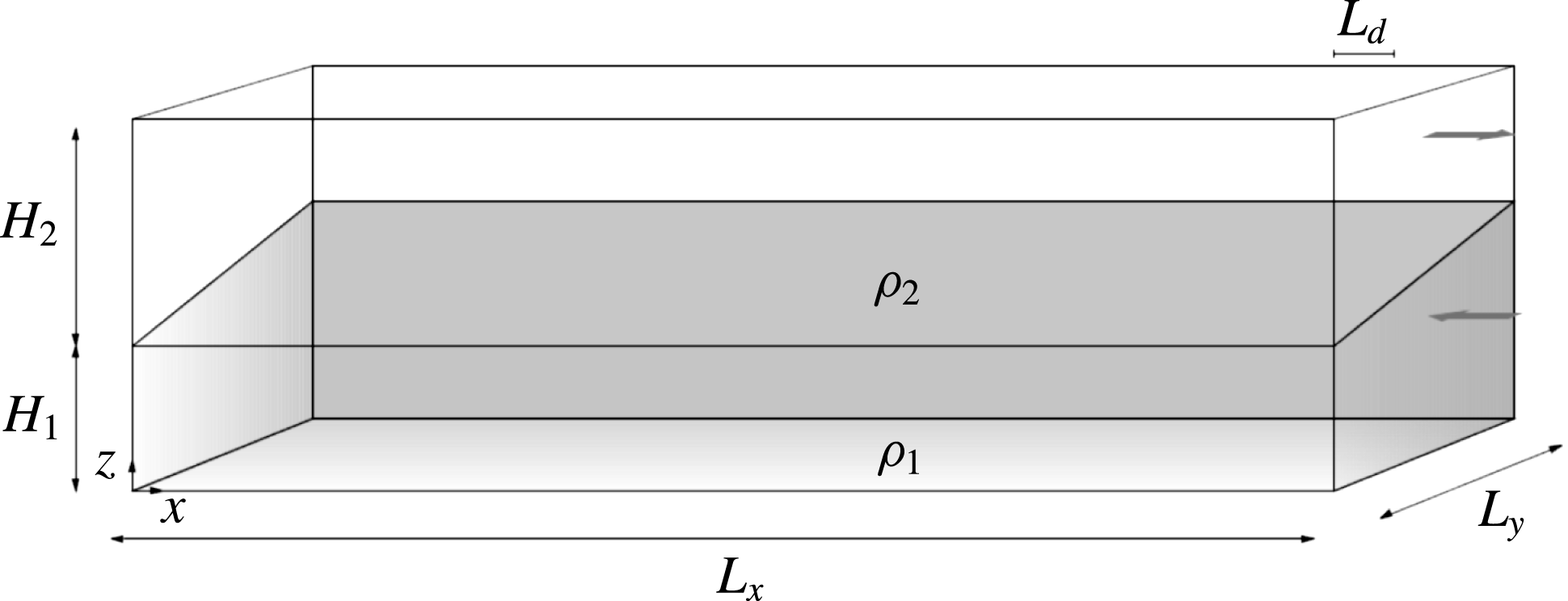
The thermal forcing of a planetary atmosphere generally varies from the equator to the poles. Equatorial regions typically receive more solar radiation than the poles (at lower levels). The resulting latitudinal temperature gradient implies a vertical gradient of the horizontal velocity, by thermal wind balance under the QG approximation. As in (Panetta & Held Reference Panetta and Held1988), this vertical shear is represented in a two-layer QG model as a uniform westward flow in the lower layer and a uniform eastward flow in the upper layer, as illustrated in figure 2. Indeed, a negative northward temperature gradient at lower levels (in the northern hemisphere) implies a positive vertical gradient of velocity, here westward in the lower layer and eastward in the upper layer. The mean zonal velocity is kept fixed at its thermal equilibrium value at the
 $y$
-boundaries. In the interior, the mean zonal velocity may vary as a result of baroclinic and barotropic instability.
Illustration of the initial undisturbed state of a two-layer quasi-geostrophic vertically sheared flow, with uniform westward flow in the lower layer and uniform eastward flow in the upper layer.

From (2.6), the QGPV is linearly related to the streamfunction, which in turn is linearly related to the velocity. Adding a uniform velocity to the flow corresponds to adding a linear streamfunction profile
 $\unicode[STIX]{x1D713}\propto y$
and hence a linear PV profile in (2.6). Thus, vertical shear corresponds to adding a linear profile to the pre-existing background PV,
 $\unicode[STIX]{x1D6FD}y$
, so that the total PV is, say,
 $\unicode[STIX]{x1D716}_{i}\unicode[STIX]{x1D6FD}y$
in each layer (
 $i=1,2$
). Below, we take
 $\unicode[STIX]{x1D716}_{1}$
to be a control parameter and deduce
 $\unicode[STIX]{x1D716}_{2}$
from the requirements that (i) the vertical shear projects only on the vertical mode with the highest deformation wavenumber (hereafter, the ‘baroclinic’ mode) and that (ii) it has zero mass average (
 $\unicode[STIX]{x1D70C}_{1}h_{1}\bar{u}_{1}+\unicode[STIX]{x1D70C}_{2}h_{2}\bar{u}_{2}=0$
). Full details may be found in appendix A.
To allow baroclinic instability, the potential vorticity gradients in the two layers must have opposite signs, implying
 $\unicode[STIX]{x1D716}_{1}\unicode[STIX]{x1D716}_{2}<0$
. Baroclinic instability however acts to reduce the vertical shear, leading to a quasi-stable flow. To prevent this and to allow cycles alternating between turbulent and quiescent states, thermal damping is imposed to help maintain the large-scale vertical shear. The thermal damping here crudely corresponds to radiative forcing by the Sun or internally. It acts to restore the layer interfaces
 $\unicode[STIX]{x1D6FF}_{i}$
to their initial thermal equilibrium profiles
 $\unicode[STIX]{x1D6FF}_{eq,i}$
at the rate
 $r$
. This leads to non-conservative changes in the QGPV through the relation between the QGPV and interface displacement, namely (2.5) with
 $\tilde{h}_{i}=(\unicode[STIX]{x1D6FF}_{i}-\unicode[STIX]{x1D6FF}_{i-1})/H_{i}$
and
 $\unicode[STIX]{x1D6FF}_{0}=0$
. To eliminate reference to
 $f_{0}$
,
 $g$
etc., it is convenient to scale the interface displacements so they have units of vorticity:
 $$\begin{eqnarray}\tilde{\unicode[STIX]{x1D6FF}}_{i}\equiv \frac{f_{0}\unicode[STIX]{x1D6FF}_{i}}{H}.\end{eqnarray}$$
Owing to the relations (2.1), together with the definition of
 $\bar{k}_{d}^{2}$
in (2.4), we can express the scaled interface displacements as
 $$\begin{eqnarray}\tilde{\unicode[STIX]{x1D6FF}}_{1}=h_{1}h_{2}\bar{k}_{d}^{2}(\unicode[STIX]{x1D713}_{1}-\unicode[STIX]{x1D6FC}\unicode[STIX]{x1D713}_{2});\quad \tilde{\unicode[STIX]{x1D6FF}}_{2}=h_{1}h_{2}\bar{k}_{d}^{2}(1-\unicode[STIX]{x1D6FC})\unicode[STIX]{x1D713}_{2}.\end{eqnarray}$$
Then, thermal damping contributes the following terms to
 $F_{1}$
and
 $F_{2}$
in (2.1):
 $$\begin{eqnarray}F_{1}\leftarrow r(\tilde{\unicode[STIX]{x1D6FF}}_{1}-\tilde{\unicode[STIX]{x1D6FF}}_{eq1})/h_{1};\quad F_{2}\leftarrow r((\tilde{\unicode[STIX]{x1D6FF}}_{2}-\tilde{\unicode[STIX]{x1D6FF}}_{1})-(\tilde{\unicode[STIX]{x1D6FF}}_{eq2}-\tilde{\unicode[STIX]{x1D6FF}}_{eq1}))/h_{2}.\end{eqnarray}$$
2.4 Boundary conditions
We employ a channel model, with periodic conditions in
 $x$
(longitude) and free-slip rigid boundaries in
 $y$
(latitude). On the
 $y$
-boundaries, the zonally averaged zonal velocity is held fixed to the value imposed by the vertical shear, as in Panetta & Held (Reference Panetta and Held1988). The model has a rigid bottom surface and a free top surface, as illustrated schematically in figure 1.
2.5 Non-dimensionalisation
We choose to employ dimensionless quantities only. To this end, we take the width of the domain to be
 $L_{x}=2\unicode[STIX]{x03C0}$
and its breadth to be
 $L_{y}=\unicode[STIX]{x03C0}$
, and, most importantly, ensure that these dimensions are much larger than the characteristic Rossby deformation length
 $L_{d}=1/\bar{k}_{d}=0.05$
. (A more representative measure of
 $L_{d}$
is
 $2\unicode[STIX]{x03C0}/\bar{k}_{d}=\unicode[STIX]{x03C0}/10$
, yet this is still much smaller than
 $L_{y}$
.) The total height of the model
 $H$
is taken to be
 $c_{\unicode[STIX]{x1D70C}}=2$
density scale heights
 $H_{\unicode[STIX]{x1D70C}}$
, corresponding to a density ratio of
 $\unicode[STIX]{x1D70C}_{2}/\unicode[STIX]{x1D70C}_{1}=\unicode[STIX]{x1D6FC}=\text{e}^{-c_{\unicode[STIX]{x1D70C}}/2}\simeq 0.37$
, although
 $c_{\unicode[STIX]{x1D70C}}=0.2$
and
 $0$
have also been studied (see below). For
 $c_{\unicode[STIX]{x1D70C}}=2$
and
 $\bar{k}_{d}=20$
, and for equal layer depths
 $h_{1}=h_{2}=0.5$
, the deformation wavenumbers of each vertical mode are
 $k_{d1}\simeq 8.87$
and
 $k_{d2}\simeq 17.93$
(see appendix A for details).
2.6 Parameter choices
We set the planetary vorticity gradient
 $\unicode[STIX]{x1D6FD}$
to be
 $8\unicode[STIX]{x03C0}$
, corresponding to a Rossby wave period of unity for a barotropic disturbance with a wavenumber of
 $4$
. Recall that the initial PV gradients in each layer are
 $\unicode[STIX]{x1D716}_{i}\unicode[STIX]{x1D6FD}$
, and the choice of
 $\unicode[STIX]{x1D716}_{1}$
controls the strength of the vertical shear. Here, we consider two main values of
 $\unicode[STIX]{x1D716}_{1}$
, namely
 $-0.1$
and
 $-0.5$
, corresponding to
 $\unicode[STIX]{x1D716}_{2}\simeq 2.81$
and
 $3.79$
respectively. For
 $\unicode[STIX]{x1D716}_{1}=-0.5$
, the initial mean velocities in the two layers are
 $\bar{u}_{1}\simeq -0.094$
and
 $\bar{u}_{2}\simeq 0.256$
(see appendix A for details). The enstrophy input rate
 $\unicode[STIX]{x1D702}$
controlling the injection of hetons ranges between
 $0.01$
and
 $100$
. We consider values of the heton PV
 $q_{heton}$
ranging from
 $1\times \unicode[STIX]{x1D6FD}/\bar{k}_{d}$
to
 $1200\times \unicode[STIX]{x1D6FD}/\bar{k}_{d}$
, whereas we fix the heton radius
 $R$
at
 $0.05$
unless otherwise stated. We vary the thermal damping rate
 $r$
between
 $0$
and
 $0.5$
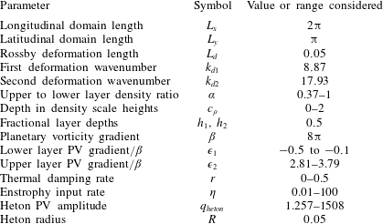
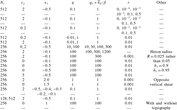
. Section 6 examines the effect of variations in the parameters. A full list of the dimensionless physical parameters and the values used are provided in table 1.
Over 100 simulations have been run using a variety of grid dimensions
 $N_{x}\times N_{y}$
, for
 $N_{x}=\{128,256,512\}$
and
 $N_{y}=N_{x}/2+1$
, over
 $10^{4}$
units of time (and up to
 $10^{5}$
units for very small
 $r$
). Note: an extra grid point is needed in the
 $y$
direction to include the boundaries and ensure each grid box is square.
2.7 Numerical model
All simulations have been carried out using the ‘combined Lagrangian advection method’ (CLAM) developed by Dritschel & Fontane (Reference Dritschel and Fontane2010). This numerical method, using a pseudo-spectral method at large scales and Lagrangian contour advection at small scales, is both highly accurate and efficient (see Dritschel & Tobias (Reference Dritschel and Tobias2012) for a recent demanding comparison). All numerical parameters follow the recommended choices outlined in Fontane & Dritschel (Reference Fontane and Dritschel2009) except that twice as many PV contour levels (here 80) are used to represent the initial PV variation in each layer. The PV contour interval remains fixed in time.
Physical parameters used in the model simulations.

3 Results
We begin by presenting in detail a characteristic flow simulation. The flow illustrated alternates, irregularly, between a more disturbed ‘turbulent’ phase and a more zonal ‘quiescent’ phase. The initial baroclinically unstable zonal state rapidly breaks down and never fully recovers. The instability equilibrates into a structured flow, a quiescent phase, where regions of nearly homogeneous PV are separated by eastward jets in the upper layer and westward jets in the lower layer. Next, and as a result of the accumulative effect of thermal damping, this structured state destabilises and breaks down, again through baroclinic instability but on a much different basic state than was present initially. The flow becomes more turbulent and much less organised. It then recovers to a structured quiescent phase only to break down again into a turbulent phase, and so on. We pay particular attention to the flow behaviour around these turbulent phases, and we study the changes in energy (kinetic/potential, zonal/eddy, barotropic/baroclinic) and zonal-flow stability which occur.
3.1 A characteristic simulation
The chosen simulation has been run on a
 $512\times 256$
‘inversion’ grid (the effective grid resolution is 16 times finer in each direction), with a thermal damping rate
 $r=0.01$
, a stratification parameter
 $c_{\unicode[STIX]{x1D70C}}=2$
, a lower layer fractional PV gradient
 $\unicode[STIX]{x1D716}_{1}=-0.5$
, a heton PV
 $q_{heton}=1\times \unicode[STIX]{x1D6FD}/\overline{k}_{d}$
and an enstrophy input rate
 $\unicode[STIX]{x1D702}=0.1$
.
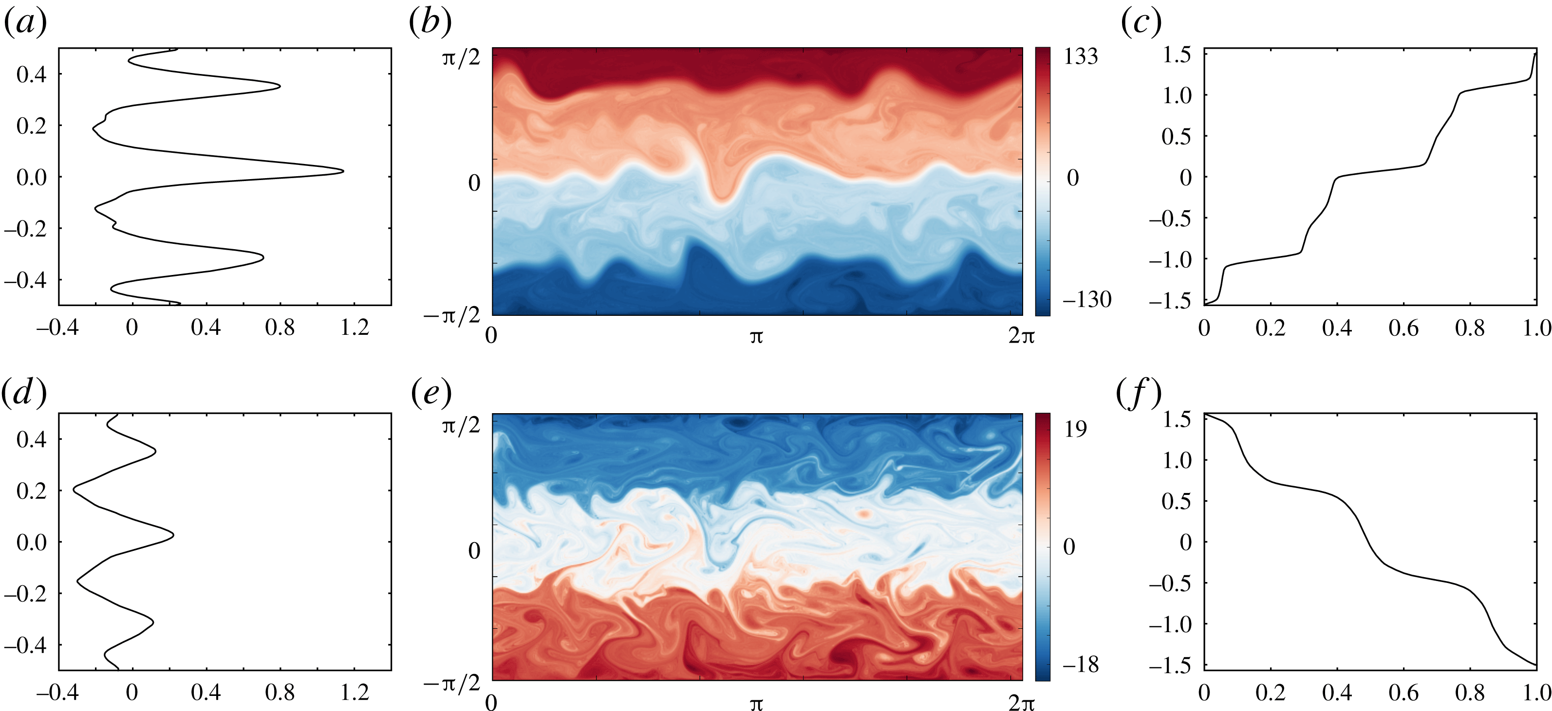
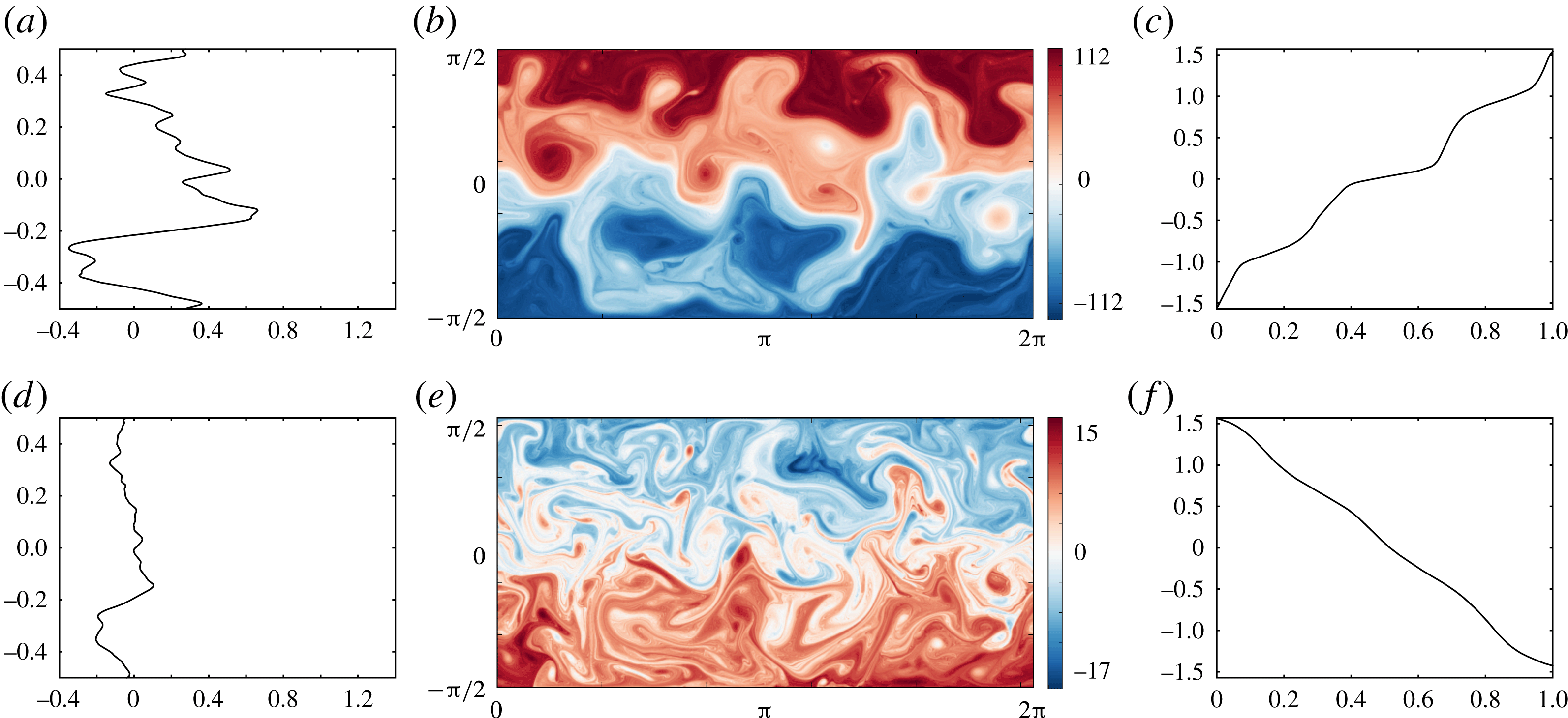
At the initial time, the flow exhibits a linear slope in PV, opposite in each layer. This flow is baroclinically unstable (as explicitly shown in appendix A), and within a few units of time leads to a strongly non-zonal, eddying turbulent flow. This subsequently collapses and organises into bands of nearly uniform PV separated by jets. This quiescent phase, illustrated in figure 3 at
 $t=3000$
typically lasts hundreds of time units, or several damping time scales
 $r^{-1}$
.
(a–c) The upper layer flow, and (d–f) the lower layer flow, all at
 $t=3000$
. (a,d) Normalised latitude
 $2y/\unicode[STIX]{x03C0}$
versus zonally averaged zonal velocity
 $\bar{u}_{i}(y,t)$
. (b,e) PV field
 $q_{i}(x,y,t)$
over the entire domain. (c,f) Equivalent latitude
 $y_{e}(\tilde{q},t)$
versus normalised PV
 $\tilde{q}=(q-q_{min})/(q_{max}-q_{min})$
.

Figure 3(b,e) shows the PV field at this time in the upper and the lower layers, respectively. In the upper layer, four distinct bands of nearly homogeneous PV are present, separated by three jets flowing eastward. In the lower layer, by contrast, there are three bands of nearly homogeneous PV separated by two westward jets. As discussed in Dritschel & McIntyre (Reference Dritschel and Mcintyre2008) and Scott & Dritschel (Reference Scott and Dritschel2012) in the context of a single-layer model, the ‘equivalent latitude’ PV profile
 $y_{e}(q)$
is particularly useful for identifying jets, here seen by the nearly flat portions of the curves shown in figure 3(c,f). The formation of a staircase profile in
 $y_{e}(q)$
indicates the presence of homogeneous regions (
 $\text{d}y_{e}/\text{d}q\rightarrow \infty$
) and jets (
 $\text{d}y_{e}/\text{d}q\rightarrow 0$
). The function
 $y_{e}(q)$
is obtained by rearranging the PV monotonically in each layer. In the upper layer,
 $y_{e}(q)=y_{min}+A_{2}(q)/L_{x}$
where
 $A_{2}(q)$
is the area occupied by PV values having
 $q>q_{min}$
. In the lower layer, where the mean PV gradient is generally reversed, instead
 $y_{e}(q)=y_{min}+A_{1}(q)/L_{x}$
where
 $A_{1}(q)$
is the area occupied by PV values having
 $q<q_{max}$
.
Figure 3(c,f) shows
 $y_{e}(\tilde{q})$
versus normalised PV, defined by
 $\tilde{q}\equiv (q-q_{min})/(q_{max}-q_{min})$
, for each layer. Both layers exhibit a near staircase profile, but it is most distinct in the upper layer. The three main small gradient portions of the curve seen here correspond to the strong eastward jets seen in the zonally averaged zonal velocity
 $\bar{u}_{2}$
(figure 3
a), while the four high gradient portions correspond to the nearly homogeneous PV regions. The zonal flow in these regions is weakly westwards. In the lower layer, the two (central) small gradient regions in
 $y_{e}(\tilde{q})$
correspond to westward jets (figure 3
d). Between the westward jets in this layer one also sees eastward jets of comparable magnitude. These are induced by the strong PV gradients in the upper layer. PV inversion couples the layers together so that the flow in either layer depends on the PV in both layers. Here however the lower layer PV is relatively weak, so it has much less impact on the upper layer flow than has the upper layer PV on the lower layer flow.
Overall, the observed jets are not vertically coherent, implying that the baroclinicity of the flow is important. The two layers have different numbers of jets. Jets flow eastward in the upper layer and predominantly westward in the lower layer. Moreover, the upper layer jets are much faster than the lower layer jets. Additionally, signatures of the jets in one layer are visible in the PV field of the other layer. In the upper layer (figure 3
b), the transitions between the two sky/pale blue bands, and between the pink-reddish bands (the two middle bands) coincide with the locations of the lower layer westward jets. These signatures appear in the equivalent latitude
 $y_{e}(\tilde{q})$
(figure 3
c) as small swerves in the middle of the two high gradient portions. In the lower layer, the signatures of the upper layer jets are less obvious, but are visible in the zonally averaged flow, an effect of PV inversion mentioned above. Jet signatures in PV are less evident in the lower layer in part because the flow is more disturbed at small scales there.
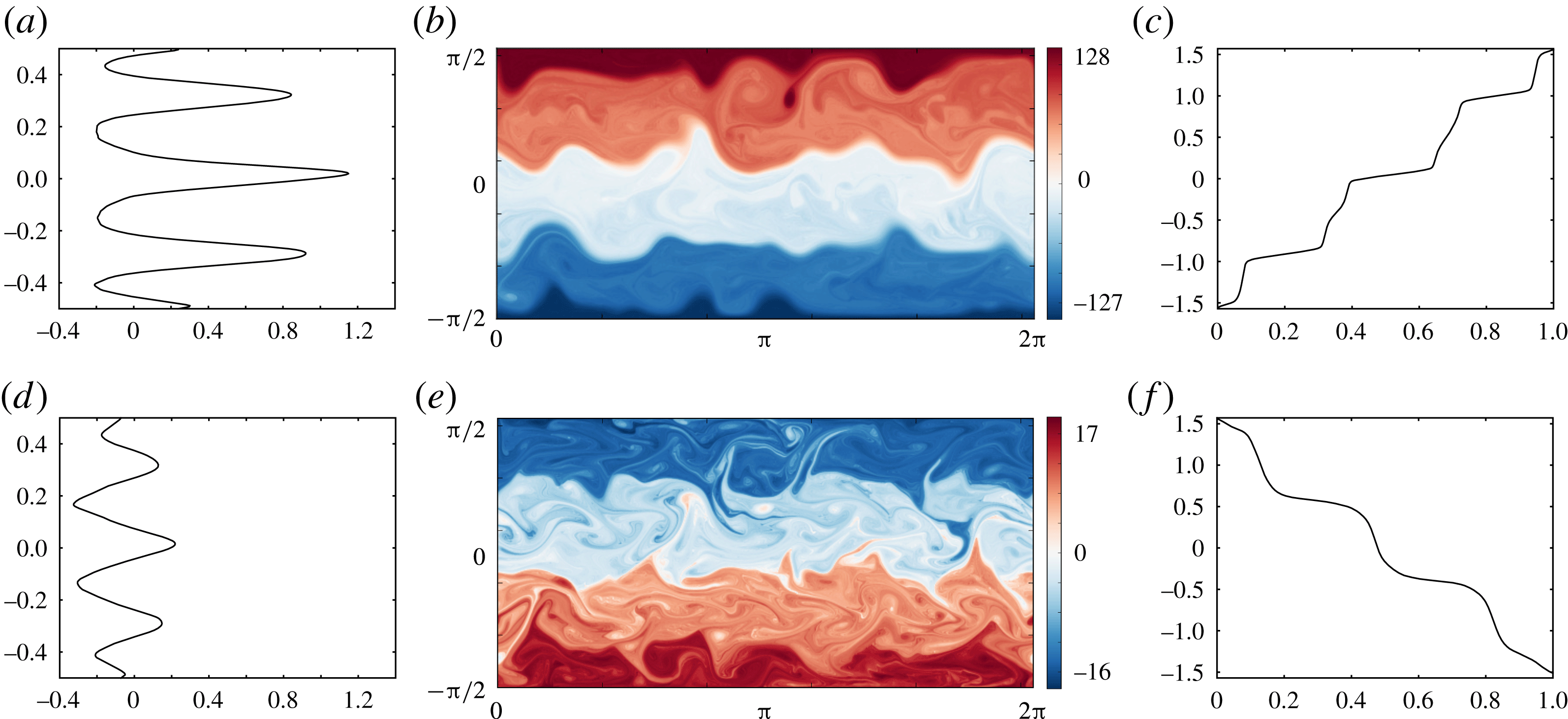
Figure 4 illustrates the same flow at a later time
 $t=4000$
, during a turbulent phase. The flow is substantially less zonal, with large-amplitude excursions exhibited in the PV field in both layers. Remarkably, nearly homogeneous regions persist in the upper layer though they are much more disturbed than in the quiescent phase. Moreover, the jets are considerably weaker and virtually absent from the lower layer flow. The ‘jets’ seen in the upper layer are not steady and show no obvious relation to the equivalent latitude PV profile
 $y_{e}(\tilde{q},t)$
. A series of short-lived vortices can be seen, especially in the central regions of the flow. These formed from the buckling and breaking of the jets at earlier times and re-merge with the jets subsequently. Two movies of the PV evolution are available in the online supplementary material available at https://doi.org/10.1017/jfm.2017.79.
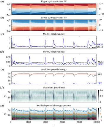
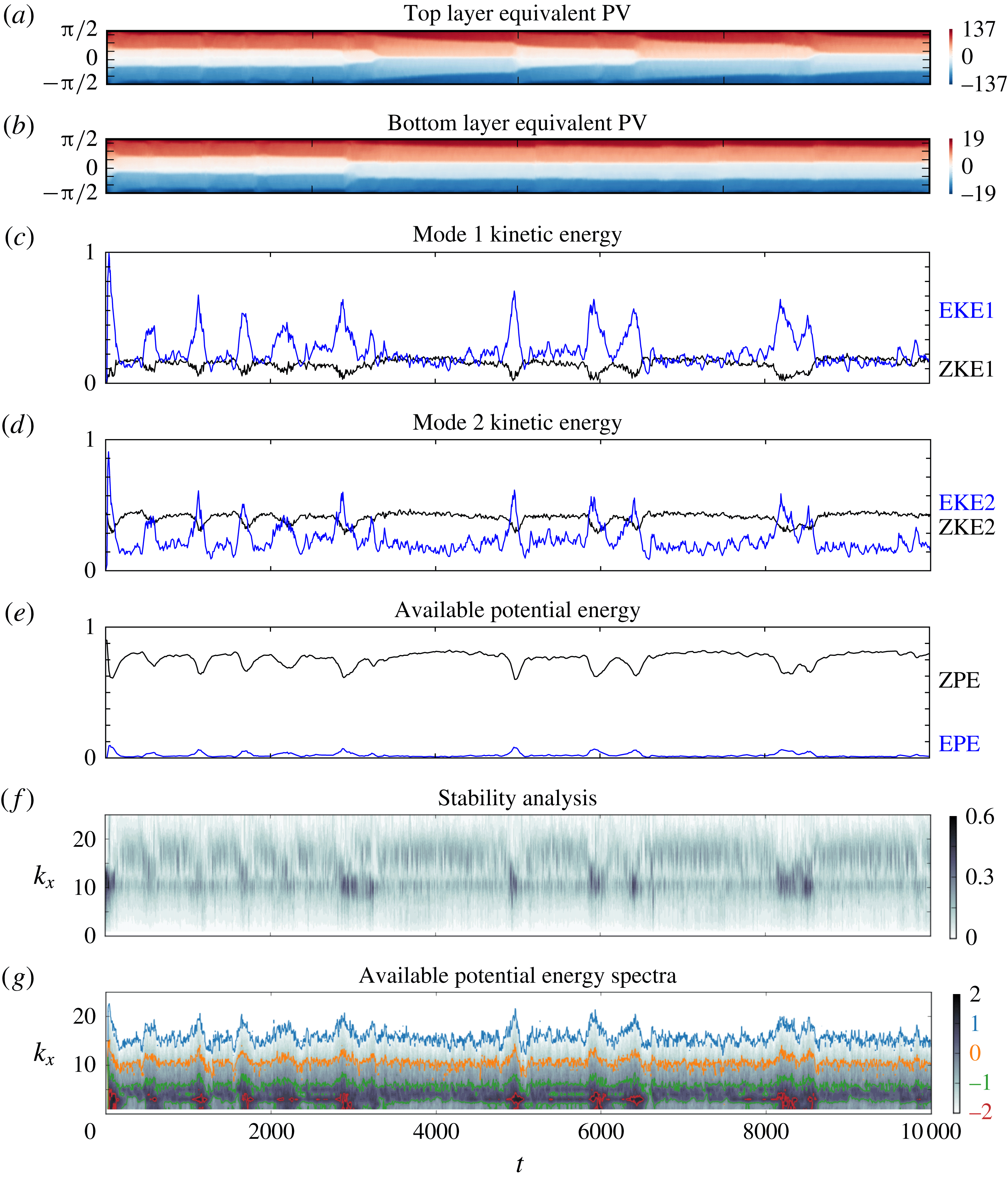
Various statistics summarising the time evolution of the flow are provided in figure 7. From top to bottom we show the equivalent PV
 $q_{e}(y)$
(the inverse of the function
 $y_{e}(q)$
) in the upper and lower layers as Hövmoller diagrams, the zonal and eddy kinetic energy in the first ‘barotropic’ and second ‘baroclinic’ vertical modes, the zonal and eddy potential energies, the maximum growth rate of the instantaneously zonally averaged flow versus zonal wavenumber, and the meridionally integrated spectrum of the available potential energy (APE) versus zonal wavenumber. In each plot, time is in the abscissa.
The equivalent PV Hövmoller diagrams (figure 7 a,b) allow one to identify major changes in the flow structure, such as a latitudinal shift of the jets and homogeneous regions. We can see here the entire evolution of the flow, starting with the first rapid reorganisation of the flow from its unstable initial state, to the alternation between quiescent phases and (relatively short) turbulent phases.
The initial linear PV variations
 $\unicode[STIX]{x1D716}_{i}\unicode[STIX]{x1D6FD}y$
are short lived after the flow destabilises and evolve into nearly homogeneous regions separated by jets, or staircase profiles, by
 $t=500$
. This is the beginning of the first quiescent phase. Four nearly homogeneous regions are clearly identifiable in the upper layer and between them three jets are present. The lower layer at this stage has three nearly homogeneous regions with two westward jets separating them. Over the next
 $1600$
units of time, the innermost homogeneous regions narrow slowly but progressively, due to the accumulative effects of thermal damping (this does not occur in the absence of damping). Near
 $t=2100$
, the quasi-zonal flow is disrupted and a short turbulent phase occurs, lasting no more than approximately 100 days, which is the thermal damping time scale,
 $r^{-1}$
. The flow then recovers, this time significantly more rapidly than it did following the initial instability, and enters a second quiescent phase, illustrated in figure 3 at
 $t=3000$
.
Over the next
 $1900$
units of time, the same progressive thinning of the innermost homogeneous regions occurs, disrupted by a turbulent phase around
 $t=4000$
, illustrated in figure 4. This sequence of long quiescent and short turbulent phases continues with irregular frequency almost to the end of the simulation. At approximately
 $t=9000$
, the flow passes through a turbulent event and organises into an anomalous quiescent phase, similar to that seen after the initial instability near
 $t=0$
, see figure 5. Instead of having a symmetric flow with a centred jet, the flow exhibits a shift of the jets and homogeneous regions as shown in figure 6.
(a–c) The upper layer flow, and (d–f) the lower layer flow, all at
 $t=4000$
. (a,d) Normalised latitude versus zonally averaged zonal velocity (note that plot scales for
 $u$
are the same as in figure 3). (b,e) PV field over the entire domain. (c,f) Equivalent latitude
 $y_{e}(\tilde{q},t)$
versus normalised PV.

(a–c) The upper layer flow, and (d–f) the lower layer flow, all at
 $t=9400$
. (a,d) Normalised latitude versus zonally averaged zonal velocity (note that plot scales for
 $u$
are the same as in figure 3). (b,e) PV field over the entire domain. (c,f) Equivalent latitude
 $y_{e}(\tilde{q},t)$
versus normalised PV.

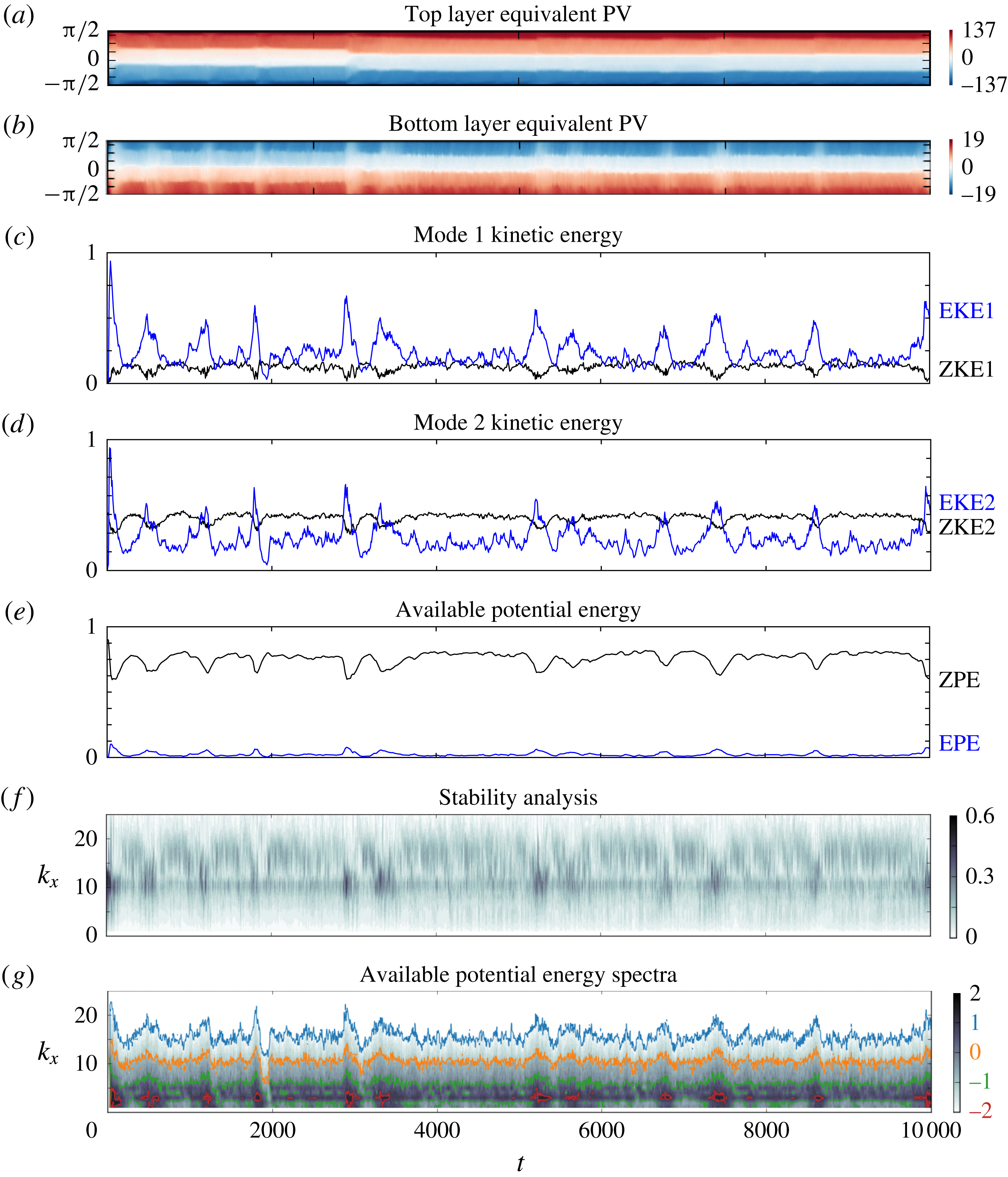
This anomalous quiescent phase is significantly more active and non-zonal than previous such phases. It is also found in other simulations and is discussed further in appendix B below.
The energy diagnostics (figure 7 c–e) closely correlate with the variations seen in the equivalent PV Hövmoller diagrams. Each turbulent phase is characterised by a strong peak in the non-zonal, eddy component of the energy and a dip in the zonal component. For the barotropic (mode 1) kinetic energy, the eddy energy (EKE1) is always comparable or greater than the zonal part (ZKE1). The baroclinic (mode 2) kinetic energy is smaller, with the eddy part (EKE2) surpassing the zonal part (ZKE2) only during turbulent phases. On the other hand, the potential energy is much larger: even the eddy potential energy (EPE) is greater than any component of the kinetic energy. The zonal potential energy (ZPE) is more than 10 times any component of kinetic energy. This dominance of ZPE is seen in all simulations conducted. Note: here we mean the APE relative to a resting basic state (APE measures the mean-square displacement of the layer interfaces).
The maximum growth rate of the instantaneous zonally averaged flow (figure 7
f) shows that the turbulent phases coincide with periods of relatively strong baroclinic instability, involving zonal wavenumbers
 $k_{x}$
mainly between 5 and 20. Note that the instability is not in fact purely baroclinic, except in the initial stages when the mean flow is a simple baroclinic shear. In general, there is a projection on the barotropic mode as well when the zonal mean flow is more complex (see e.g. (James Reference James1987), who examined the influence of barotropic shear on baroclinic instability). It appears that the instability precedes the growth in the eddy energy components, but in fact it occurs after these components have already grown significantly (this is shown below in detail). Hence, it is too simplistic to think that the thermal damping has led to an unstable zonal-flow state, which then becomes turbulent. The non-zonal flow must also play a role, but this cannot be assessed simply through a linear stability analysis.
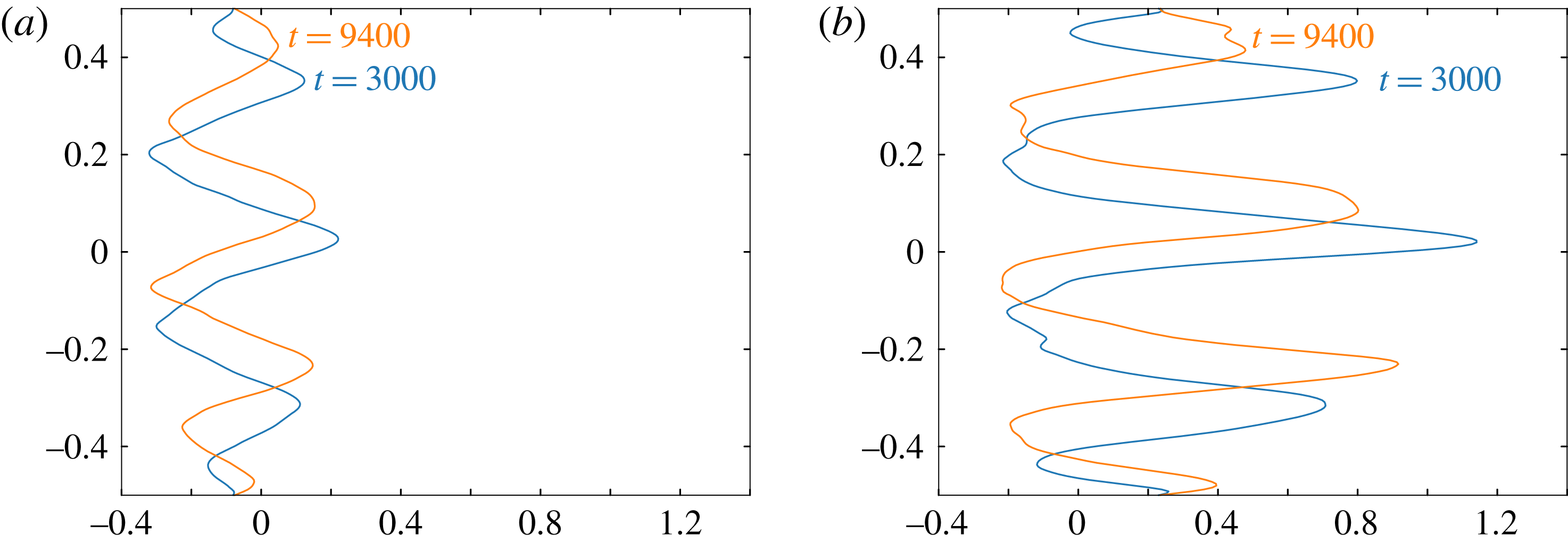
Lower layer (a) and upper layer (b) zonally averaged zonal velocity
 $\bar{u}_{i}(y,t)$
at two different times
 $t=3000$
blue and
 $t=9400$
orange.

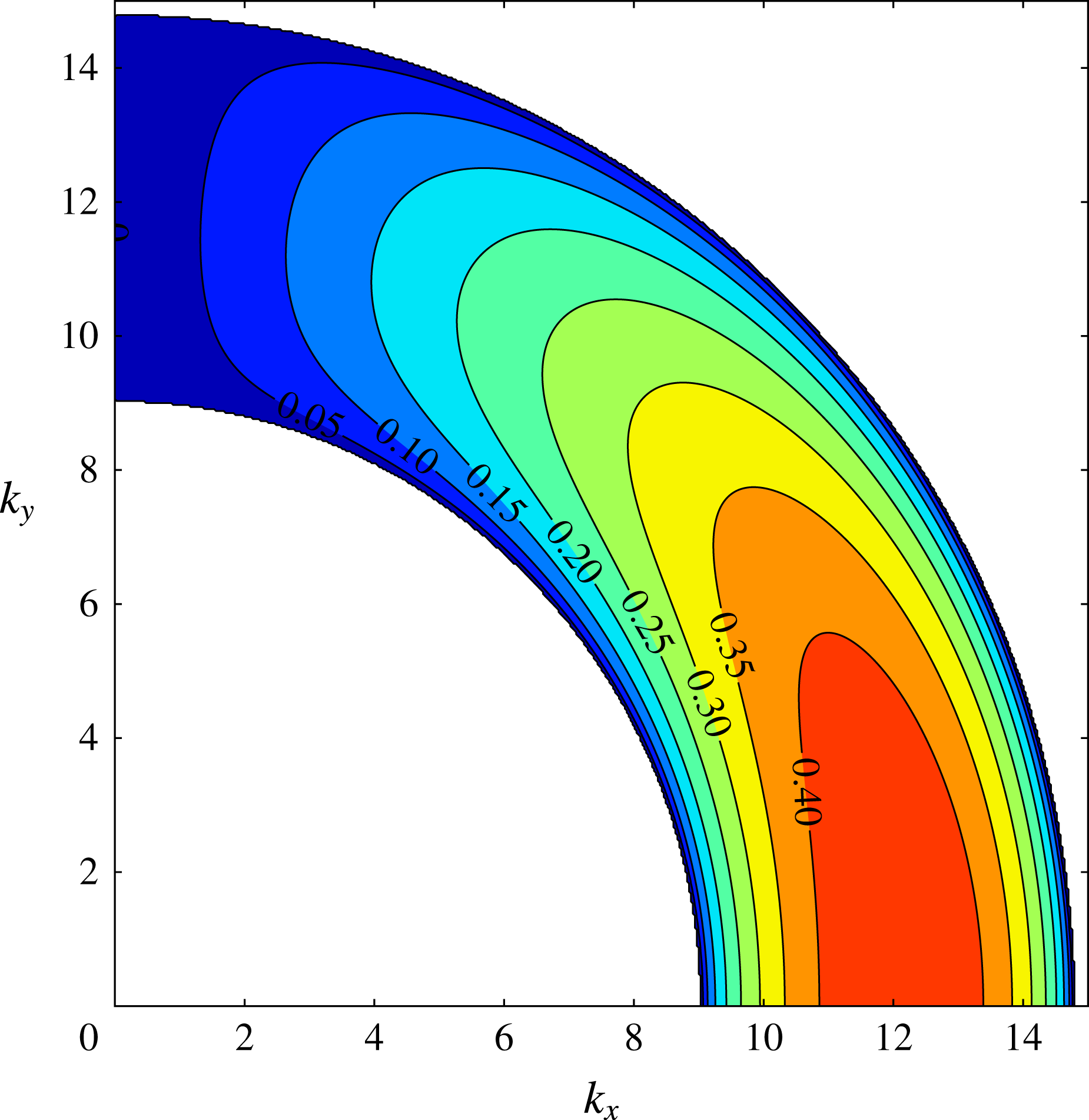
Finally, in figure 7(g) we show the meridionally integrated APE spectrum as a function of zonal wavenumber
 $k_{x}$
(between
 $1$
and
 $25$
) and time. At the very earliest stages,
 $t\leqslant 10$
, baroclinic instability excites wavenumbers centred on
 $k_{x}=11$
(as found in the linear stability analysis). Very soon after, a broad spectrum of disturbances emerges, with dominant power residing at much lower wavenumbers, around
 $k_{x}=4$
and to a lesser extent
 $k_{x}=6$
. This is typical of quiescent phases, and indicates a significant and persistent amount of eddy activity even during these phases. The turbulent phases on the other hand are characterised by the excitation of a broad range of wavenumbers, both lower and higher. This spreading is characteristic of turbulent flow evolution. Each turbulent phase appears to first spread APE to higher wavenumbers then build up energy at low wavenumbers, predominantly
 $k_{x}=2$
and
 $3$
. This is short lived however as the flow returns to a quiescent phase.
(a,b) Hövmoller diagrams of the equivalent PV
 $q_{e}(t,y)$
, with latitude in the ordinate. (c–e) Energy components (with the eddy part in blue, the zonal part in black and the red line the time-averaged APE). (f)
 $\log _{10}$
of the maximum growth rate of the zonally averaged flow versus zonal wavenumber
 $k_{x}$
. (g)
 $\log _{10}$
of the meridionally integrated spectrum of available potential energy versus zonal wavenumber
 $k_{x}$
. The coloured contours correspond to specific values of the spectrum as indicated on the colour bar. In all of these plots time is in the abscissa.

4 Energy transfers
We next look more closely at the energy transfers taking place between different energy components (kinetic/potential, barotropic/baroclinic, zonal/eddy) to gain a better understanding of the flow changes occurring when entering and leaving turbulent phases. To be more quantitative, we define a turbulent phase as a period when the ZPE is smaller than the mean ZPE. Other definitions have been tried, but this simple definition adequately identifies turbulent phases, as seen in figure 7.
To study energy transfers, we examine two different kinds of instantaneous correlations between the six energy components ZKE1, ZKE2, ZPE, EKE1, EKE2 and EPE. Note that it is not possible to express the rate of change of any one component solely in terms of the other components, so one must seek other means to examine the energy transfers taking place. We have chosen correlations, separated into turbulent and quiescent phases, together with directions of energy change, as explained below.
The first correlation is the standard one, defined for two time series
 $\{x_{1},x_{2},\ldots ,x_{n}\}$
and
 $\{y_{1},y_{2},\ldots ,y_{n}\}$
by
 $$\begin{eqnarray}r_{xy}=\frac{\displaystyle \mathop{\sum }_{i=1}^{n}(x_{i}-\bar{x})(y_{i}-\bar{y})}{\sqrt{\displaystyle \mathop{\sum }_{i=1}^{n}(x_{i}-\bar{x})^{2}\mathop{\sum }_{i=1}^{n}(y_{i}-\bar{y})^{2}}},\end{eqnarray}$$
where
 $\bar{x}=n^{-1}\sum _{i=1}^{n}x_{i}$
and
 $\bar{y}=n^{-1}\sum _{i=1}^{n}y_{i}$
. The second one, which we call the ‘global correlation’, is defined by the numerator of (4.1) only. This gives a better measure of the energy magnitudes involved and, in particular, helps to identify the key components involved in the energy transfers taking place. In the results presented, data have been sampled every 5 units of time, providing energy time series of
 $n=2001$
values.
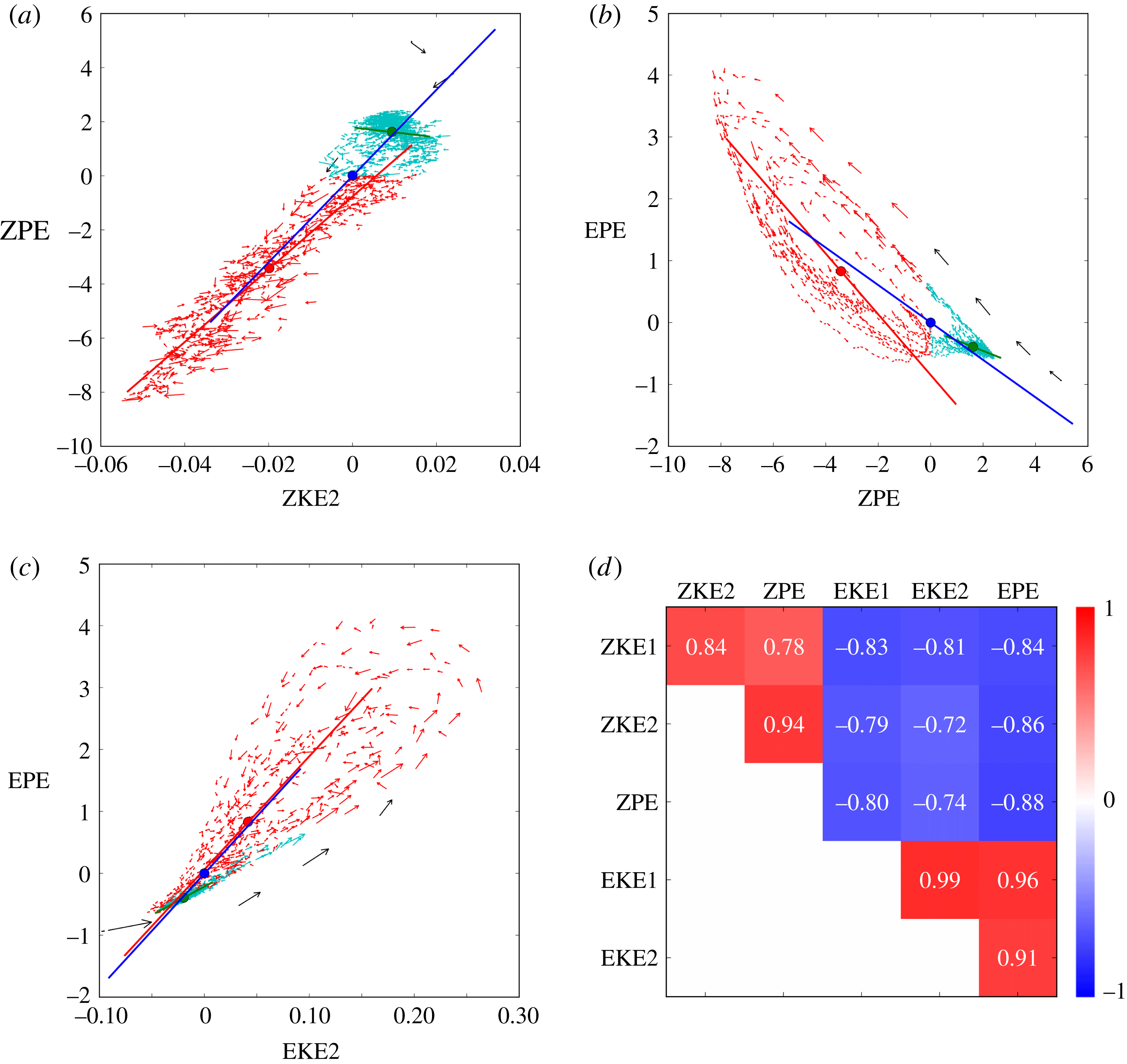
(a–c) Scatterplots of different energy components in the characteristic simulation, for (a) ZPE versus ZKE2, (b) EPE versus ZPE and (c) EPE versus EKE2. Note: the mean values are subtracted and the scales are adjusted to the range of energy values observed. The arrows represent a third of the distance between adjacent points. Black arrows: initial phase. Cyan arrows: quiescent phases. Red arrows: turbulent phases. The lines show the best fit of the data (cyan for quiescent phases, red for turbulent phases and blue overall), after optimal rotation of the data and a least-squares fit. The lengths of the lines are proportional to the spread in the data. (d) The standard correlation matrix is shown, computed using (4.1) for the different energy components.

Figure 8 shows three scatterplots of different energy components and the standard correlation matrix. First, the correlation matrix exhibits three distinct areas. The two red areas show that zonal energies are positively correlated with each other, and that eddy energies are also positively correlated with each other. The blue area shows that zonal energies are negatively correlated with eddy energies. This finding agrees with that found in figure 7 for the evolution of the energy components, namely that when there is a decrease of any zonal energy the other zonal energies also decrease and the eddy energies increase and vice versa.
In the scatterplots, further information can be obtained. First of all, we see the strong, tight correlation between ZKE2 and ZPE (figure 8
a), consistent with the value of
 $0.94$
seen in the correlation matrix. Moreover, the eddy energies are all tightly and positively correlated (only EKE2 versus EPE is presented here in figure 8
c). The scatterplots exhibit a racquet shape, very narrow at the base, corresponding to the quiescent phases, and more spread at the top, corresponding to the turbulent phases. Moreover, there is a definite pattern of evolution: the flow leaves a quiescent phase with relatively low EPE, gains EPE during the peak of the turbulent phase then returns to the quiescent phase with relatively high EPE.
Similar looping patterns are present in the zonal versus eddy and in the ZKE1 versus zonal scatterplots. These patterns are more widely spread than seen between the eddy energies themselves. If we look at ZPE versus EPE (figure 8 b), we see that ZPE diminishes as EPE grows when leaving a quiescent phase, following nearly a straight line. It then returns along a curved line to recover from a turbulent phase. During this recovery, EPE falls relatively quickly while ZPE does not show much growth until near the end of the turbulent phase. This slow recovery of ZPE is likely due to the weak thermal damping. The nearly straight lines, leaving quiescent phases and entering turbulent phases, are all closely parallel. The more eccentric one, with black arrows, corresponds to the initial stages where baroclinic instability acts on an idealised basic state. All the other straight lines are parallel to this one because the same phenomenon happens: ZPE is converted into EPE due to baroclinic instability. However the zonal energy at the beginning of subsequent turbulent phases is lower than it was in the initial phase, explaining the gap between the different lines.
A difficulty in the interpretation of these results arises because the scatterplots are two-dimensional projections of a six-dimensional phase space. The loop patterns seen imply that other components, not shown in a given two-dimensional cross-section, are involved in the energy transfers taking place, and moreover that the transfers are not occurring simultaneously (this is highlighted in § 5). An alternative interpretation, discussed next, focuses on the energy components exhibiting the greatest variations.
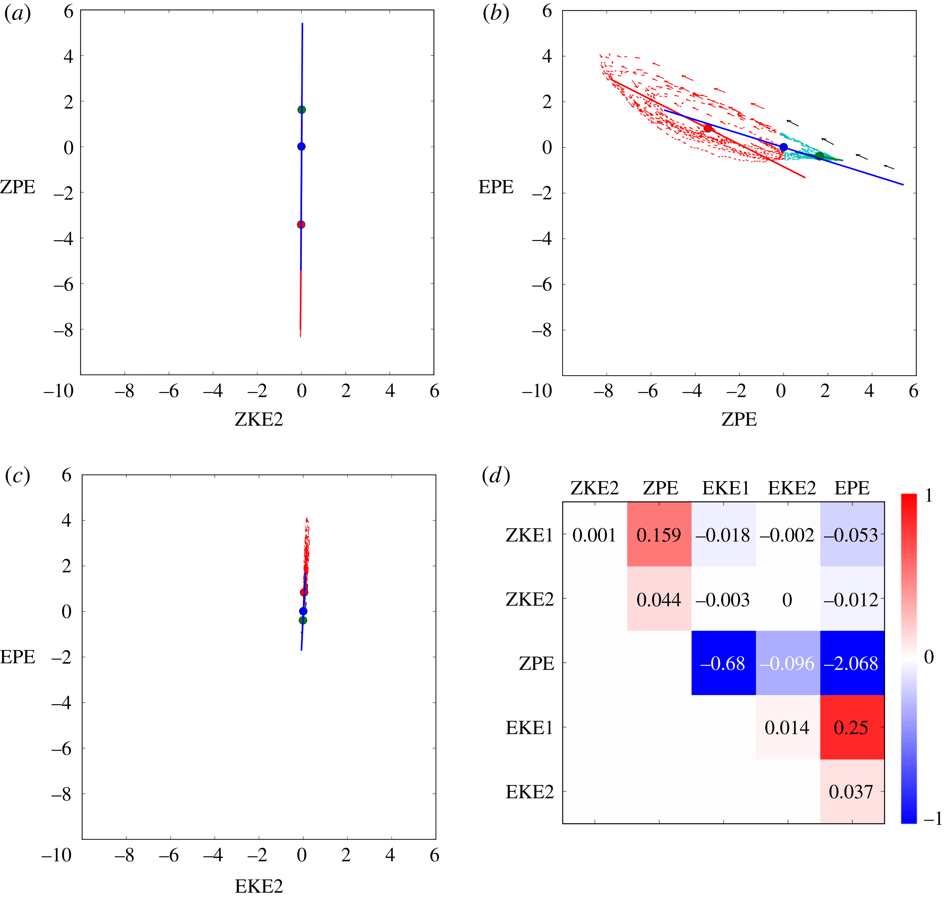
(a–c) Scatterplots of different energy components, (a) for ZPE versus ZKE2, (b) for EPE versus ZPE, (c) for EPE versus EKE2, in the characteristic simulation as in table 1 but using fixed, identical scales in each plot to emphasise which energy components exhibit the greatest variations. (d) The global correlation matrix is shown, computed using only the numerator of (4.1) for the different energy components.

The standard correlation scatterplots in figure 8 show the correlation between different energy components, but not the energy transfer. To see the energy transfer, it is necessary to use the same plot limits in all scatterplots and to correlate the energy components using only the numerator of (4.1). These global correlations are exhibited in figure 9 in the same format as figure 8 for comparison. The main energy transfers involve just a few components, ZPE, EPE and to a weaker extent EKE1 and ZKE1. The other components have essentially no impact on the global energy transfer. In particular, some components which show a strong standard correlation instead show a very weak global correlation, such as ZKE2 versus ZPE. This means that ZKE2 and ZPE evolve similarly but there is scarcely any energy transfer between them.
The dominant energy transfer occurs between ZPE and EPE and is strongly anti-correlated, as expected. ZPE is also anti-correlated with EKE1, implying that both EPE and EKE1 are the dominant components uptaking any change in ZPE. This is consistent also with the positive correlation between EPE and EKE1. Finally, and perhaps surprisingly, only one correlation between zonal energies, ZPE versus ZKE1, is notable. For a relatively large gain in ZPE, there is a modest increase in ZKE1. Evidently, the thermal restoration of the sloping layer interfaces favours an increase in barotropic energy. Restoration of a linear slope would not have this effect, as a linear slope only generates a baroclinic flow, by construction. Instead, it must be that the eddying motions present even during quiescent phases continue to provide inhomogeneous PV mixing, maintaining sharp jets (Dritschel & McIntyre Reference Dritschel and Mcintyre2008; Scott & Dritschel Reference Scott and Dritschel2012). These jets project on both barotropic and baroclinic modes, unlike the initial vertical shear flow.
5 Focus on a turbulent phase
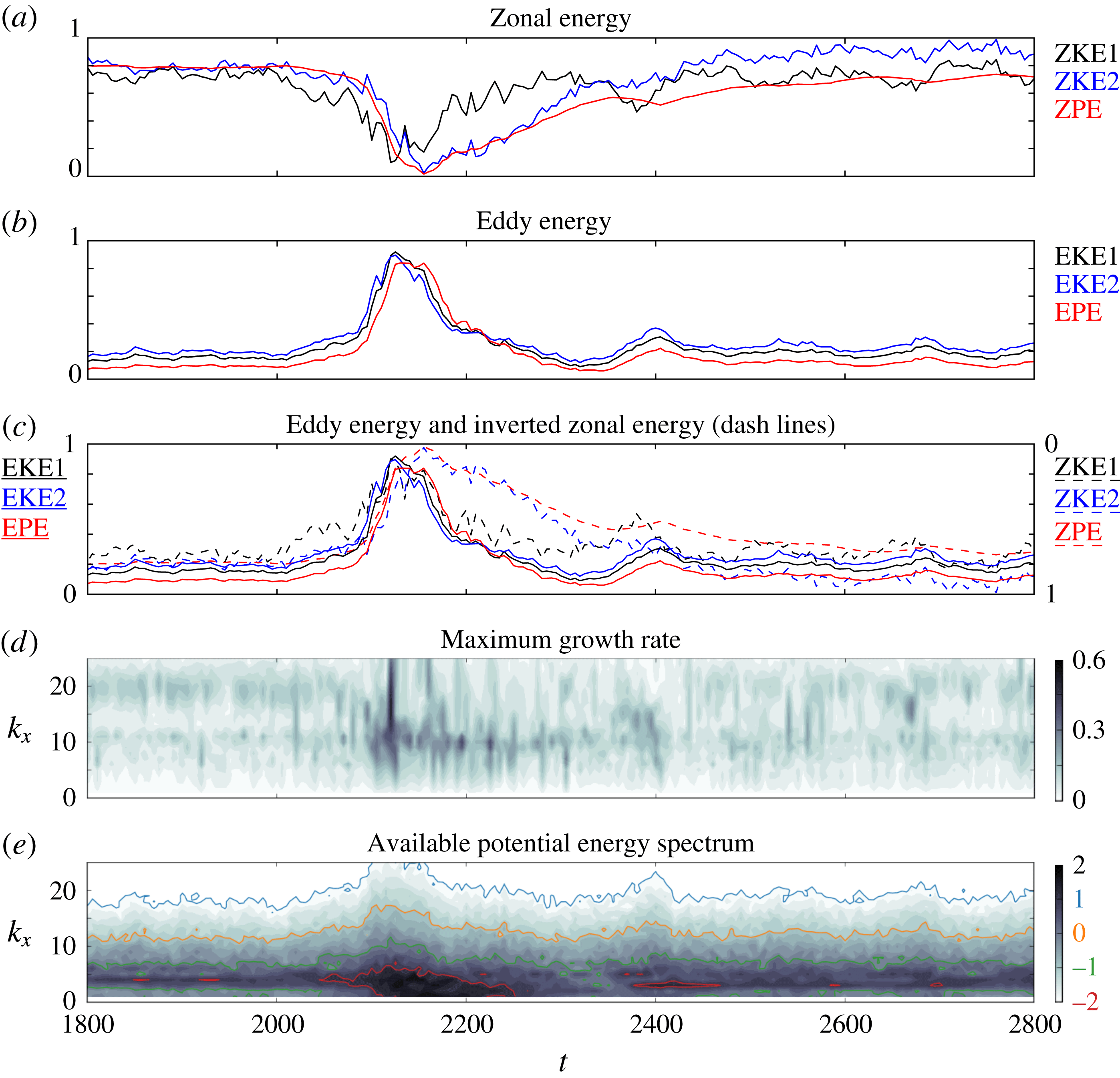
The detailed behaviour of the flow around a turbulent phase is examined in this section. The panels in figure 10 show the time evolution of various diagnostics over
 $1800\leqslant t\leqslant 2800$
. Figure 10(a–c) shows energy components linearly rescaled to lie between
 $0$
and
 $1$
over the entire simulation duration (
 $0\leqslant t\leqslant 10\,000$
). In figure 10(c), the complement of the rescaled zonal energies is shown so that they can be better compared with the rescaled eddy energies (c combines a and b). Figure 10(d) shows the maximum growth rate for each zonal wavenumber
 $k_{x}$
(in the abscissa), and figure 10(e) shows the meridionally integrated APE spectrum, also versus
 $k_{x}$
.
(a–c) Rescaled energy components (with mode 1 kinetic energy in black, mode 2 kinetic energy in blue and available potential energy in red) versus time for
 $1800\leqslant t\leqslant 2800$
. In (a) only zonal components are shown, in (b) only eddy components are shown, while in (c) all components are shown with the zonal ones inverted for comparison. (d)
 $\log _{10}$
of the maximum growth rate of the zonally averaged flow versus zonal wavenumber
 $k_{x}$
. (e)
 $\log _{10}$
of the meridionally integrated spectrum of the available potential energy versus
 $k_{x}$
. The coloured contours correspond to specific values of the spectrum as indicated on the colour bar. In each panel, time is in the abscissa.

In figure 10(a), the rescaled zonal energies ZKE2 and ZPE follow the same trend, especially on the approach to the turbulent phase. This is why the standard correlation between ZKE2 and ZPE is very high. However, ZKE1 decreases before the two other energies and recovers sooner. Similarly, in figure 10(b) for the rescaled eddy energies, there is a small offset between the different components. EKE1 and EKE2 grow first (with EKE2 slightly ahead) and next EPE follows, with almost the same trend. This offset between the different energy components explains the looping or racquet patterns observed in the standard correlation scatterplots in table 1.
Figure 10(c) compares the rescaled zonal and eddy energies. This highlights the differences in evolution of the various components. The eddy energies are seen to rise and fall rapidly, over a time scale comparable but shorter than the damping period
 $r^{-1}=100$
. The mode 1 zonal kinetic energy ZKE1 appears to lead all components into the turbulent phase, but due to the rescaling, the energy changes involved are actually smaller than those taking place in ZPE and EPE (cf. figure 7). The onset of the turbulent phase is best associated with the steep rise in all the curves just before
 $t=2100$
, with the dominant energy transfer between ZPE and EPE. Other rising events happen later, e.g. between
 $t=2300$
and
 $2400$
, without leading to any major disruption of the flow.
It therefore appears that the disturbance must reach a threshold amplitude before triggering a turbulent phase (this has been confirmed by examining many such events). In the PV field (not shown, but see the movie available to the online supplementary material), wave amplitudes along the jets are seen to slowly grow, eventually (sometimes after several false starts) leading to wave breaking and vortex formation. This strongly disturbed state lasts only a relatively short time before the vortices are either torn apart by the jet shear or recaptured by the jets, and the wave amplitudes gradually subside. The slow return to a quiescent state is most apparent in the behaviour of ZPE and ZKE2: the thermal damping slowly acts to rebuild the sloping layer interfaces, at the same time enhancing the baroclinic shear (in ZKE2). In this return to a quiescent phase, the principal energy changes (i.e. in ZPE) are mainly brought about by thermal damping. However, the rapid decay in all eddy energies, occurring over a period of just
 $20$
to
 $30$
units of time, cannot be explained simply by thermal damping. Instead, part of this decay must be due to inhomogeneous turbulent mixing, constrained by the mean PV gradient in each layer. The mixing acts to homogenise PV and sharpen jets, processes which are only enhanced by non-zonal variations (Dritschel & McIntyre Reference Dritschel and Mcintyre2008; Scott & Dritschel Reference Scott and Dritschel2012). The mixing continues until most of the eddy energy (principally at higher wavenumbers where thermal damping is weak) is exhausted and converted into jets (qualitatively this is the argument behind the Rhines scale
 $L_{Rh}=\sqrt{U/\unicode[STIX]{x1D6FD}}$
, where
 $U$
characterises the eddy velocities and
 $\unicode[STIX]{x1D6FD}$
is the background PV gradient, see Rhines (Reference Rhines1975)). The low wavenumber part of the eddy energy gives rise to meanders, which unlike the high wavenumber part are affected by the thermal damping. Subsequently, thermal damping weakens the meanders and establishes quasi-zonal jets around
 $t=2200$
. Thereafter, thermal damping gradually modifies them, slowly bringing them closer together at the centre of the channel, as seen in figure 7(a,b). Eventually, this sets up the conditions for a further turbulent phase.
The maximum growth rate of the flow (shown in figure 10
d) increases in the expected range of baroclinic instability wavenumbers, i.e. wavenumbers around
 $k_{x}=11$
, at the onset of the turbulent phase. Thereafter, at the peak of the turbulent phase around
 $t=2150$
, a wide range of wavenumbers are excited. Notably, just before this peak there is a decrease in the growth rate for high wavenumbers (18–20), that will only recover during the next quiescent phase. While it is not very clear in this figure, this feature is common to all the turbulent phases.
The APE spectrum (figure 10
e) before the turbulent phase shows significant and persistent excitation of wavenumbers 4–6. During the first part of the turbulent phase, there is an increase in power for small wavenumbers, from
 $2$
to
 $4$
, and more generally for all wavenumbers. This is the effect of wave breaking, vortex generation and subsequent turbulent mixing. The increased excitation of all wavenumbers is matched by the growth of EPE shown in figure 10(b). Likewise, as the excitation subsides, so does the EPE, reaching a minimum around the end of the turbulent phase at
 $t=2350$
.
From this analysis, we can better understand the energy variations occurring during the onset and decay of a turbulent phase. The loop patterns exhibited in the correlation scatterplots (cf. table 1) are associated with the asynchronous growth and decay of the various energy components. What we find generically, across many events and simulations examined, is that at the onset of a turbulent phase ZKE1 decreases marginally sooner than both ZKE2 and ZPE, which remain highly correlated until near the end of the turbulent phase. ZKE1 recovers much sooner than either ZKE2 or ZPE, and this appears to be an eddy effect. Looking back at figure 7, we can see that the dips in ZKE1 occurring during a turbulent phase only last while there is significant eddy energy. By contrast, ZKE2 and ZPE take longer to recover, well after the eddy energies have all but dissipated. Another generic feature worth noting is that, at the onset of a turbulent phase, EKE2 appears to increase slightly before EKE1, which is then followed by EPE. The recovery is also in the same order, with EPE recovering last. The recovery is also rapid, mainly a nonlinear effect of inhomogeneous mixing. Thermal damping acts most strongly at largest scales, and gradually weakens the low wavenumber meanders on the jets. This helps to re-establish strong quasi-zonal jets, which then slowly shift due to thermal damping until conditions are established for the next turbulent phase.
6 Dependence on parameters
6.1 Parameter sweep
To study the dependence of the flow evolution on the different parameters involved, a wide range of simulations have been conducted. The main parameters consist of the thermal damping coefficient
 $r$
, the lower layer fractional PV gradient
 $\unicode[STIX]{x1D716}_{1}$
(directly controlling the vertical shear), the stratification coefficient
 $c_{\unicode[STIX]{x1D70C}}$
, the enstrophy input rate
 $\unicode[STIX]{x1D702}$
and the heton PV
 $q_{heton}$
. Other parameters have been varied, like the heton radius
 $R$
and topographic forcing, but these have been found to have only a minor influence. Table 2 lists the parameters used for the main simulations conducted in this study. In the following subsections, we focus on the parameters having the greatest influence: the thermal damping
 $r$
and the vertical shear parameter
 $\unicode[STIX]{x1D716}_{1}$
. We then briefly summarise the influence of the remaining parameters.
Numerical and physical parameters for the set of experiments conducted in this study.

6.2 Thermal damping
An important parameter controlling the flow evolution is thermal damping. A wide range of thermal damping rates
 $r=\{0,0.0001,0.001,0.01,0.1,0.5\}$
have been examined, mainly for different values of stratification coefficient
 $c_{\unicode[STIX]{x1D70C}}$
and vertical shear parameter
 $\unicode[STIX]{x1D716}_{1}$
. Thermal damping acts to restore the initial vertical shear. Simultaneously, baroclinic instability, induced by excessive vertical shear, leads to turbulent mixing which tends to reduce the vertical shear. There is thus a competition between thermal damping and baroclinic instability which nearly always results in the formation of jets through inhomogeneous PV mixing.
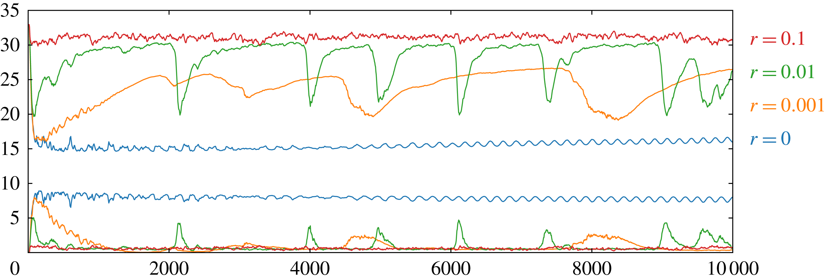
The evolution of zonal (upper plots) and eddy (lower plots) potential energy (ZPE and EPE) for different thermal damping rates
 $r$
: no damping, black;
 $0.001$
, blue;
 $0.01$
(reference), red; and
 $0.1$
, green.

Thermal damping is found to have a major impact on the evolution of the flow. This is exhibited in figure 11 comparing the evolution of zonal potential energy (ZPE) for
 $r=0$
,
 $0.001$
,
 $0.01$
and
 $0.1$
, keeping all other parameters at their default values. The green curve corresponds to the characteristic simulation examined already. At high damping rates,
 $r\geqslant 0.1$
, the flow appears to be very stable: the initial ZPE is reduced by only 12 % for
 $r=0.1$
and fluctuates close to a constant value thereafter. In fact, small-scale disturbances are ever present due to the perpetual creation of baroclinic instability, but no large-scale disruption like that seen in figure 4 for the characteristic simulation ever occurs. At high damping, the flow exhibits many weak jets whose number remains constant from the earliest times. By contrast, with no damping (
 $r=0$
), the imposed vertical shear is rapidly cancelled, suppressing any further baroclinic instability. The flow in this case is mainly dominated by large-scale oscillations with a few weak jets, see figure 12. For small but non-zero damping (
 $r=0.001$
and
 $0.01$
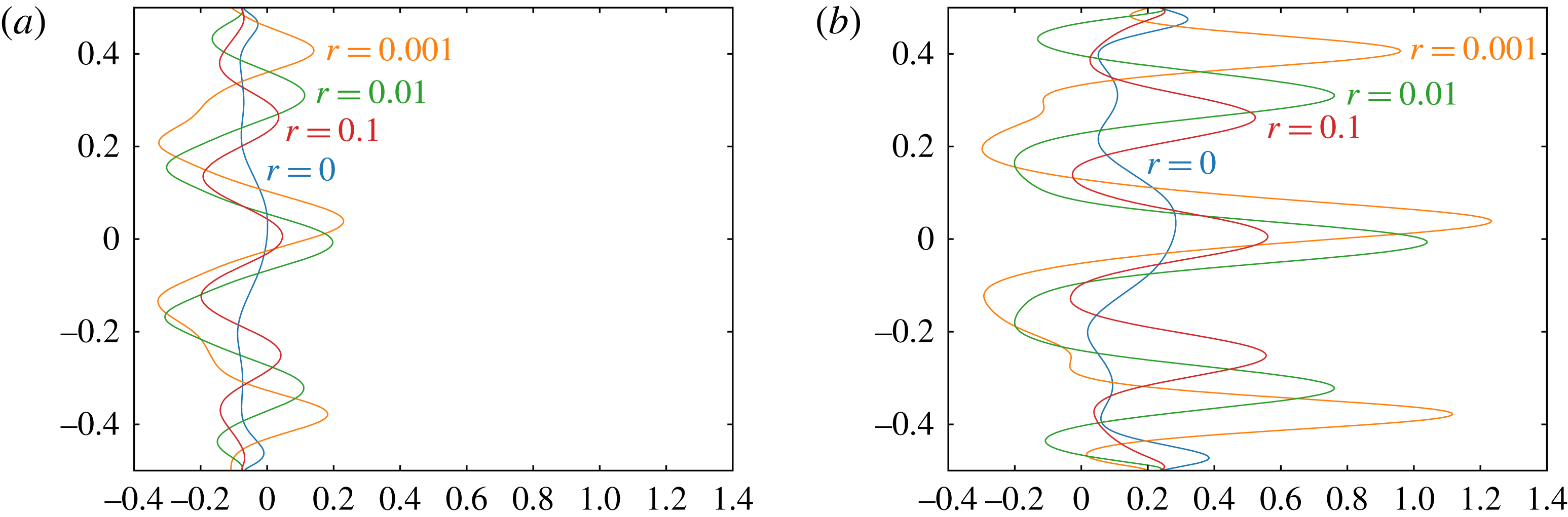
), there is a competition between the damping trying to restore the vertical shear and baroclinic instability trying to break it down, leading to strong, widely spaced jets. The damping has a direct impact on the intensity of the jets (their zonal velocity) and jet spacing, as seen in figure 12. As in the characteristic case presented in § 3.1, the flow is more unstable and variable, and exhibits large-scale fluctuations. The damping rate strongly affects the recovery time from each turbulent phase, leading to a wider spacing of turbulent events.
6.3 Vertical shear
The initial vertical shear is directly controlled by the lower layer relative PV gradient,
 $\unicode[STIX]{x1D716}_{1}$
(see appendix A). When
 $\unicode[STIX]{x1D716}_{1}<0$
, PV gradients are reversed in the two layers, and the vertical shear is sufficient to induce baroclinic instability. The more negative
 $\unicode[STIX]{x1D716}_{1}$
is, the greater is the vertical shear and thus the potential for instability.
The time averaged – between
 $t=6500$
and
 $t=7300$
– (quiescent phase) zonally averaged zonal velocity
 $\bar{u}_{i}(y,t)$
for the lower layer (a) and the upper layer (b), for different thermal damping rates
 $r$
: no damping, black;
 $0.001$
, blue;
 $0.01$
(reference), red; and
 $0.1$
, green.

Zonal potential available energy’s evolution for five different vertical shears
 $\unicode[STIX]{x1D716}_{1}$
:
 $-0.1$
brown;
 $-0.2$
purple;
 $-0.3$
red;
 $-0.4$
green; and
 $-0.5$
orange and blue.

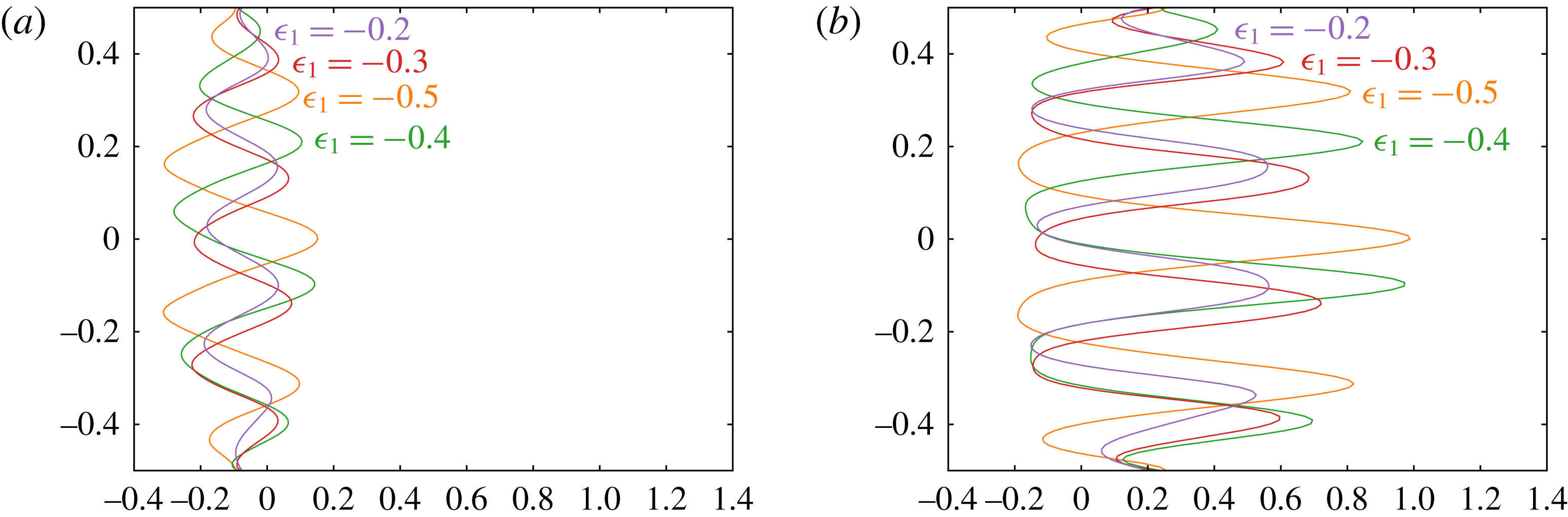
Lower layer (a) and upper layer (b) zonally averaged zonal velocity
 $\bar{u}_{i}(y,t)$
averaged between
 $t=3800$
and
 $4500$
(quiescent phase), for different vertical shears
 $\unicode[STIX]{x1D716}_{1}$
:
 $-0.2$
purple;
 $-0.3$
red;
 $-0.4$
green; and
 $-0.5$
orange.

Vertical shear has a direct influence on the number of homogeneous regions and jets that develop, see figure 13. Increased vertical shear implies stronger baroclinic instability and thus higher root mean square eddy velocities,
 $u_{rms}^{\prime }$
. This on its own would imply an increased jet spacing, qualitatively, through the Rhines scale
 $L_{Rh}=\sqrt{u_{rms}^{\prime }/|\bar{q}_{y}|}$
, except that the mean PV gradient
 $|\bar{q}_{y}|$
also increases. Nevertheless, we find that higher vertical shear leads to both a wider jet spacing and more intense jets, see figure 14. Regarding the oscillations between quiescent and turbulent phases, higher vertical shear decreases their frequency. When the vertical shear is too weak to permit baroclinic instability (
 $\unicode[STIX]{x1D716}_{1}\geqslant 0$
), the flow evolution is radically different than what we have seen so far. Jets, if at all present, are very weak and erratic.
6.4 Other parameters
Many other simulations have been conducted, looking at the effect of stratification, the PV of the injected hetons, the enstrophy input rate, etc. Regarding stratification, the simulations presented in this paper are relevant to an atmospheric-like situation. We have also run simulations for oceanic-like cases (
 $c_{\unicode[STIX]{x1D70C}}\rightarrow 0$
). The main difference is a greater propensity for meandering at small scales, such as seen in oceanic currents like the Kuroshio or the Gulf Stream. Large-scale structures are still present, though they are weaker and significantly disturbed by small-scale perturbations. Jets are also less prominent. As in the oceans, the flow is less structured into zonal bands but contains many more coherent vortices. These findings are broadly consistent with those found by Maximenko et al. (Reference Maximenko, Bang and Sasaki2005), Kamenkovich et al. (Reference Kamenkovich, Berloff and Pedlosky2009), Berloff et al. (Reference Berloff, Karabasov, Farrar and Kamenkovich2011) who examined a forced idealised two-layer ocean with Ekman damping.
Regarding the heton PV and the enstrophy input rate, we have examined the effect of adding a few high intensity hetons versus adding numerous low intensity hetons. We thought that adding high intensity hetons would favour the formation of long-lived vortices, but this is not true. Inevitably any intense vortices which do form drift north or south and get torn apart by or incorporated into the intense jets. Overall, these parameters have only a small impact on the flow evolution. Simulations with different parameters exhibit the same number of homogeneous regions and jets, with comparable jet velocities and spacing.
7 Conclusions
We have investigated the emergence, nonlinear dynamics and energetics of jets and vortices in a two-layer
 $\unicode[STIX]{x1D6FD}$
-plane quasi-geostrophic channel model. An extensive range of numerical simulations have been carried out using the combined Lagrangian advection model (Dritschel & Fontane Reference Dritschel and Fontane2010), at unprecedented resolution and for very long times (
 $10^{4}$
–
 $10^{5}$
model days). We have primarily focused on the atmospheric case where there is a strong density difference between the two layers and where thermal damping acts to maintain vertical shear against baroclinic instability. As found in the original study of this type by Panetta & Held (Reference Panetta and Held1988), the competition between damping and baroclinic instability results in quasi-zonal jets. In the present study, additionally, we have included the effect of stochastic forcing, specifically adding small-scale baroclinic vortices called ‘hetons’ randomly at a prescribed enstrophy input rate. These hetons are meant to crudely model the effects of convection thought to occur in the atmospheres of the gas giant planets (see Thomson & McIntyre (Reference Thomson and Mcintyre2016) and references therein). The details of the stochastic forcing however do not seem to matter: qualitatively similar evolution is observed without such forcing when the initial flow is weakly perturbed.
The combination of thermal damping, heton forcing and atmospheric stratification leads to a ‘baroclinic life cycle’ (see Feldstein & Held Reference Feldstein and Held1989; Thorncroft, Hoskins & McIntyre Reference Thorncroft, Hoskins and Mcintyre1993; Esler Reference Esler2008), in which jets emerge through baroclinic instability of the vertically sheared flow and subsequently break down and reform, often in an irregular manner. The jets form through inhomogeneous potential vorticity mixing (Dritschel & McIntyre Reference Dritschel and Mcintyre2008; Scott & Dritschel Reference Scott and Dritschel2012), in which potential vorticity is nearly homogenised in bands, but between which the potential vorticity abruptly jumps, forming a ‘staircase’ profile. Each jump is associated with a jet, eastward in the upper layer and westward in the lower layer, a direct effect of potential vorticity inversion (Dritschel & McIntyre Reference Dritschel and Mcintyre2008).
Both thermal damping and heton forcing continuously modify the jets that form through baroclinic instability. Thermal damping works to increase the vertical shear (favouring baroclinic instability), while heton forcing creates disturbances which eventually trigger the breakdown of the jets. In most cases, this breakdown is characterised by wave amplification and breaking on the quasi-zonal jets, leading to vortex detachment and turbulence. In this ‘turbulent phase’, the upper layer jets often persist but become strongly non-zonal and time dependent, while the lower layer jets are nearly obliterated before they reform. The turbulent phase lasts typically one thermal damping period, approximately, but only part of the recovery is due to thermal damping. From a detailed analysis of the energetics, it is found that the eddies (or non-zonal disturbances) created at the onset of a turbulent phase convert their energy into jets, arguably by inhomogeneous potential vorticity mixing (an inviscid mechanism). Thermal damping, by contrast, acts mainly at large scales to dampen long-wave disturbances and straighten the jets. Thereafter, thermal damping slowly shifts the jets and builds the mean vertical shear, setting up the conditions for subsequent instability and breakdown.
Each turbulent phase is followed by a ‘quiescent’ phase characterised by nearly zonal jets with weak small-scale disturbances. These quiescent phases often exhibit a gradual latitudinal migration of the jets. In one particular example studied in detail, two distinct quiescent phases were observed, one of which was significantly more robust (long lived) than the other (further analysis may be found in appendix B.) The quasi-zonal jets occurring during the quiescent phases are typically highly baroclinic. There are different numbers of jets in each layer located at different mean latitudes. Moreover, the upper layer jets are predominantly eastward, while the lower layer jets are predominantly westward, or a mix between the two due to the strong influence of the upper layer potential vorticity on both layers.
The wider dependence of the flow evolution on thermal damping, vertical shear, stratification, heton intensity and enstrophy input rate has also been studied. Increasing thermal damping weakens the turbulence created during baroclinic instability, leading to less temporal variation especially of the zonal energy components. While baroclinic instability still occurs (for sufficient vertical shear), it only manages to create weak jets for strong thermal damping (i.e. for a 10 day or shorter damping period). On the other hand, no damping results in the destruction of the initial vertical shear and no further chance for baroclinic instability. Weaker damping leads to baroclinic life cycles, here oscillations between turbulent and quiescent phases. Both phases extend in proportion to the damping period, though the recovery of the zonal part is significantly slower than the recovery of the eddy part.
Increasing vertical shear makes the flow more unstable, generally creating fewer, more intense jets. Changing the stratification to a form more appropriate to the oceans, we find that the jets exhibit significant meandering and are less well defined. Moreover, many more vortices are present which last for much longer times than found for atmospheric stratification. These results are consistent with the two-layer ocean study of Maximenko et al. (Reference Maximenko, Bang and Sasaki2005), Kamenkovich et al. (Reference Kamenkovich, Berloff and Pedlosky2009), Berloff et al. (Reference Berloff, Karabasov, Farrar and Kamenkovich2011). The remaining model parameters (heton intensity, enstrophy input rate) have been found to have only a weak impact on the flow evolution.
A conspicuous feature of the atmospheric-like simulations we have conducted is the absence of long-lived vortices, despite an extensive exploration of parameter space. Vortices do form but they inevitably collide with a jet and are either incorporated or destroyed. A major question then is: is there a parameter regime within this two-layer quasi-geostrophic model favouring long-lived vortices? Or, is it necessary to go beyond the quasi-geostrophic model and consider ageostrophic effects (e.g. as in a shallow-water context)? Or again, is spherical geometry fundamental? Does the Great Red Spot, for instance, depend on its proximity to the equatorial region, whose dynamics can be starkly different from quasi-geostrophic? Are two-layers sufficient? We are presently working to answer some of these questions by building and applying a highly accurate multi-layer shallow-water numerical model.
Acknowledgements
The authors wish to acknowledge the LabEx
 $OSUG@2020$
and the University of St Andrews for the funding of T.J.
Supplementary movies
Supplementary movies are available at https://doi.org/10.1017/jfm.2017.79.
Appendix A. Layer model decomposition and related analyses
A.1 Vertical modes
The inversion of (2.6) for the layer streamfunctions
 $\unicode[STIX]{x1D713}_{1}$
and
 $\unicode[STIX]{x1D713}_{2}$
is accomplished through a projection onto vertical modes, i.e.
 $$\begin{eqnarray}\left.\begin{array}{@{}c@{}}\hat{\unicode[STIX]{x1D713}}_{1}=c_{11}\unicode[STIX]{x1D713}_{1}+c_{12}\unicode[STIX]{x1D713}_{2},\\ \hat{\unicode[STIX]{x1D713}}_{2}=c_{21}\unicode[STIX]{x1D713}_{1}+c_{22}\unicode[STIX]{x1D713}_{2},\end{array}\right\}\end{eqnarray}$$
where a hat indicates a vertical mode, and the
 $c_{ij}$
are the projection coefficients, determined as follows. Using the same projection for the PV anomaly
 $q_{i}^{\prime }-\unicode[STIX]{x1D6FD}y$
in (2.6), we obtain
 $$\begin{eqnarray}\hat{q}_{j}^{\prime }=\unicode[STIX]{x1D6FB}^{2}\hat{\unicode[STIX]{x1D713}}_{j}+c_{j1}h_{2}\bar{k}_{d}^{2}(\unicode[STIX]{x1D6FC}\unicode[STIX]{x1D713}_{2}-\unicode[STIX]{x1D713}_{1})+c_{j2}h_{1}\bar{k}_{d}^{2}(\unicode[STIX]{x1D713}_{1}-\unicode[STIX]{x1D713}_{2})\end{eqnarray}$$
for each vertical mode (
 $j=1$
or
 $2$
). The objective is to make the terms involving
 $c_{j1}$
and
 $c_{j2}$
equal to
 $-\unicode[STIX]{x1D6FE}_{j}\bar{k}_{d}^{2}\hat{\unicode[STIX]{x1D713}}_{j}$
for each
 $j$
, since then we have simple Helmholtz-type equations to invert for
 $\hat{\unicode[STIX]{x1D713}}_{j}$
, namely
 $$\begin{eqnarray}\hat{q}_{j}^{\prime }=\unicode[STIX]{x1D6FB}^{2}\hat{\unicode[STIX]{x1D713}}_{j}-k_{dj}^{2}\hat{\unicode[STIX]{x1D713}}_{j},\end{eqnarray}$$
where
 $k_{dj}^{2}\equiv \unicode[STIX]{x1D6FE}_{j}\bar{k}_{d}^{2}$
is the squared deformation wavenumber for mode
 $j$
. Equating then the terms above with
 $-\unicode[STIX]{x1D6FE}_{j}\bar{k}_{d}^{2}\hat{\unicode[STIX]{x1D713}}_{j}$
and rearranging, we obtain
 $$\begin{eqnarray}[(\unicode[STIX]{x1D6FE}_{j}-h_{2})c_{j1}+h_{1}c_{j2}]\unicode[STIX]{x1D713}_{1}+[(\unicode[STIX]{x1D6FE}_{j}-h_{1})c_{j2}+\unicode[STIX]{x1D6FC}h_{2}c_{j1}]\unicode[STIX]{x1D713}_{2}=0.\end{eqnarray}$$
As this must be true for all
 $\unicode[STIX]{x1D713}_{1}(x,y,t)$
and
 $\unicode[STIX]{x1D713}_{2}(x,y,t)$
, the constant coefficients must vanish:
 $$\begin{eqnarray}\displaystyle & \displaystyle (\unicode[STIX]{x1D6FE}_{j}-h_{2})c_{j1}+h_{1}c_{j2}=0, & \displaystyle\end{eqnarray}$$
 $$\begin{eqnarray}\displaystyle & \displaystyle (\unicode[STIX]{x1D6FE}_{j}-h_{1})c_{j2}+\unicode[STIX]{x1D6FC}h_{2}c_{j1}=0. & \displaystyle\end{eqnarray}$$
The only non-trivial solution results by taking the determinant of this linear system to be zero, leading to
 $$\begin{eqnarray}\unicode[STIX]{x1D6FE}_{j}^{2}-\unicode[STIX]{x1D6FE}_{j}+(1-\unicode[STIX]{x1D6FC})h_{1}h_{2}=0,\end{eqnarray}$$
which gives the prefactor
 $\unicode[STIX]{x1D6FE}_{j}$
in
 $k_{dj}^{2}\equiv \unicode[STIX]{x1D6FE}_{j}\bar{k}_{d}^{2}$
:
 $$\begin{eqnarray}\unicode[STIX]{x1D6FE}_{1,2}={\textstyle \frac{1}{2}}\mp \sqrt{{\textstyle \frac{1}{4}}-(1-\unicode[STIX]{x1D6FC})h_{1}h_{2}}.\end{eqnarray}$$
We have taken the minus sign in front of the square root for the lower mode, since it is purely ‘barotropic’ with
 $\unicode[STIX]{x1D6FE}_{1}=0$
in the Boussinesq limit
 $\unicode[STIX]{x1D6FC}\rightarrow 1$
. The other mode is called ‘baroclinic’ and always has the higher deformation wavenumber. Note:
 $\unicode[STIX]{x1D6FE}_{1}+\unicode[STIX]{x1D6FE}_{2}=1$
.
Regarding the projection coefficients
 $c_{j1}$
and
 $c_{j2}$
, by convention we take
 $c_{11}+c_{12}=1$
for the ‘barotropic’ mode
 $j=1$
. This, along with (A 5) gives
 $$\begin{eqnarray}c_{11}=\frac{h_{1}}{1-\unicode[STIX]{x1D6FE}_{1}}=\frac{h_{1}}{\unicode[STIX]{x1D6FE}_{2}};\quad c_{12}=1-\frac{h_{1}}{\unicode[STIX]{x1D6FE}_{2}}.\end{eqnarray}$$
For the ‘baroclinic’ mode
 $j=2$
, we take
 $c_{22}=1$
. Again using (A 5), we find
 $$\begin{eqnarray}c_{21}=\frac{h_{1}}{h_{2}-\unicode[STIX]{x1D6FE}_{2}};\quad c_{22}=1.\end{eqnarray}$$
The inverse of these coefficients are needed to express modes in terms of layers, i.e. as
 $$\begin{eqnarray}\left.\begin{array}{@{}c@{}}\unicode[STIX]{x1D713}_{1}=\tilde{c}_{11}\hat{\unicode[STIX]{x1D713}}_{1}+\tilde{c}_{12}\hat{\unicode[STIX]{x1D713}}_{2},\\ \unicode[STIX]{x1D713}_{2}=\tilde{c}_{21}\hat{\unicode[STIX]{x1D713}}_{1}+\tilde{c}_{22}\hat{\unicode[STIX]{x1D713}}_{2}.\end{array}\right\}\end{eqnarray}$$
Simple algebra leads to
 $$\begin{eqnarray}\tilde{c}_{11}=\frac{c_{22}}{\unicode[STIX]{x1D6E5}};\quad \tilde{c}_{12}=-\frac{c_{12}}{\unicode[STIX]{x1D6E5}};\quad \tilde{c}_{21}=-\frac{c_{21}}{\unicode[STIX]{x1D6E5}};\quad \tilde{c}_{22}=\frac{c_{22}}{\unicode[STIX]{x1D6E5}},\end{eqnarray}$$
where
 $\unicode[STIX]{x1D6E5}=c_{11}c_{22}-c_{12}c_{21}$
.
A.2 Vertical shear
A vertical shear (a uniform flow
 $\bar{u}_{i}$
in each layer
 $i$
) is imposed by taking the lower layer mean PV to be
 $\bar{q}_{1}=-\unicode[STIX]{x1D716}_{1}\unicode[STIX]{x1D6FD}y$
, specifying
 $\unicode[STIX]{x1D716}_{1}$
, and requiring the mass-integrated momentum to be zero, or
 $h_{1}\bar{u}_{1}+\unicode[STIX]{x1D6FC}h_{2}\bar{u}_{2}=0$
. The latter requirement determines the constant
 $\unicode[STIX]{x1D716}_{2}$
in the associated upper layer PV
 $\bar{q}_{1}=\unicode[STIX]{x1D716}_{2}\unicode[STIX]{x1D6FD}y$
, as well as the mean flows
 $\bar{u}_{1}$
and
 $\bar{u}_{2}$
, as explained next.
We start with (2.6) for the mean flow, for which
 $\bar{\unicode[STIX]{x1D713}}_{i}=-\bar{u}_{i}(y-y_{c})$
, where
 $y_{c}$
is the centreline of the channel. For this flow, the relative vorticity
 $\unicode[STIX]{x1D6FB}^{2}\bar{\unicode[STIX]{x1D713}}_{i}$
is zero. After cancelling the common
 $y$
factor and some rearrangement, (2.6) implies
 $$\begin{eqnarray}\left.\begin{array}{@{}c@{}}(1-\unicode[STIX]{x1D716}_{1})\unicode[STIX]{x1D6FD}=h_{2}\bar{k}_{d}^{2}(\unicode[STIX]{x1D6FC}\bar{u}_{2}-\bar{u}_{1}),\\ (1-\unicode[STIX]{x1D716}_{2})\unicode[STIX]{x1D6FD}=h_{1}\bar{k}_{d}^{2}(\bar{u}_{1}-\bar{u}_{2}).\end{array}\right\}\end{eqnarray}$$
We can solve these for the mean flows
 $\bar{u}_{1}$
and
 $\bar{u}_{2}$
in terms of
 $\unicode[STIX]{x1D716}_{1}$
and
 $\unicode[STIX]{x1D716}_{2}$
, but we also want to obtain
 $\unicode[STIX]{x1D716}_{2}$
from the condition of zero momentum,
 $h_{1}\bar{u}_{1}+\unicode[STIX]{x1D6FC}h_{2}\bar{u}_{2}=0$
. Omitting the details, this gives
 $\unicode[STIX]{x1D716}_{2}=1+(1-\unicode[STIX]{x1D716}_{1})G_{1}/G_{2}$
where
 $G_{j}=c_{1j}\unicode[STIX]{x1D6FE}_{2}+\unicode[STIX]{x1D707}c_{2j}\unicode[STIX]{x1D6FE}_{1}$
with
 $$\begin{eqnarray}\unicode[STIX]{x1D707}=\frac{h_{1}\tilde{c}_{12}+\unicode[STIX]{x1D6FC}h_{2}\tilde{c}_{22}}{h_{1}\tilde{c}_{11}+\unicode[STIX]{x1D6FC}h_{2}\tilde{c}_{21}}.\end{eqnarray}$$
The mean velocities
 $\hat{\bar{u}}_{j}$
associated with each mode
 $j$
are
 $$\begin{eqnarray}\hat{\bar{u}}_{1}=\frac{(1-\unicode[STIX]{x1D716}_{1})\unicode[STIX]{x1D6FD}\unicode[STIX]{x1D6E5}}{\bar{k}_{d}^{2}G_{2}};\quad \hat{\bar{u}}_{2}=-\unicode[STIX]{x1D707}\hat{\bar{u}}_{1},\end{eqnarray}$$
from which we obtain the mean layer velocities by projection:
 $$\begin{eqnarray}\bar{u}_{i}=\tilde{c}_{i1}\hat{\bar{u}}_{1}+\tilde{c}_{i2}\hat{\bar{u}}_{2}\quad i=1,2.\end{eqnarray}$$
A.3 Thermal equilibrium interface slopes
Initially, the flow is in thermal equilibrium, with uniform velocity
 $\bar{u}_{i}$
in each layer
 $i$
. Associated with this flow, by thermal wind balance, the layer interfaces adopt a linear profile
 $\unicode[STIX]{x1D6FF}_{eq,i}\propto y-y_{c}$
. In terms of the scaled displacements
 $\tilde{\unicode[STIX]{x1D6FF}}_{eq,i}=f_{0}\unicode[STIX]{x1D6FF}_{eq,i}/H$
, upon using their definitions in terms of streamfunctions (2.9), we find
 $$\begin{eqnarray}\tilde{\unicode[STIX]{x1D6FF}}_{eq,1}=-h_{1}h_{2}\bar{k}_{d}^{2}(\bar{u}_{1}-\unicode[STIX]{x1D6FC}\bar{u}_{2})(y-y_{c});\quad \tilde{\unicode[STIX]{x1D6FF}}_{eq,1}=-h_{1}h_{2}\bar{k}_{d}^{2}(1-\unicode[STIX]{x1D6FC})\bar{u}_{2}(y-y_{c}).\end{eqnarray}$$
These are the profiles to which the interfaces are relaxed to subsequently, at a specified rate
 $r$
.
A.4 Linear stability
We next provide brief details of the linear stability analysis used in the main body of the paper to calculate the maximum growth rate. We start with the instantaneous zonally averaged PV
 $\bar{q}_{i}$
and zonal velocity
 $\bar{u}_{i}$
in each layer
 $i=1,2$
. In this subsection, these profiles are general functions of
 $y$
for each sampled time
 $t$
. In the numerical code, they are provided at each
 $y$
grid point (typically
 $129$
or
 $257$
grid points, including the edges). The PV gradient
 $\text{d}\bar{q}_{i}/\text{d}y$
, needed in the analysis below, is computed using centred differences in
 $y$
. Notably, only the interior grid point values are needed, since the perturbation satisfies homogeneous boundary conditions (required to ensure zero meridional velocity at each boundary).
In the linear stability analysis, the base flow is considered to be both
 $x$
and
 $t$
-independent. Hence, we can consider infinitesimal perturbations of the form
 $$\begin{eqnarray}\left.\begin{array}{@{}c@{}}q_{i}^{\prime }(x,y,t)=\text{Re}\{Q_{i}(y)\text{e}^{\text{i}(k_{x}x-\unicode[STIX]{x1D70E}t)}\},\\ \unicode[STIX]{x1D713}_{i}^{\prime }(x,y,t)=\text{Re}\{\unicode[STIX]{x1D6F9}_{i}(y)\text{e}^{\text{i}(k_{x}x-\unicode[STIX]{x1D70E}t)}\},\end{array}\right\}\end{eqnarray}$$
where
 $k_{x}$
is a prescribed zonal wavenumber (necessarily integer for a domain of length
 $L_{x}=2\unicode[STIX]{x03C0}$
),
 $\unicode[STIX]{x1D70E}$
is the frequency (the imaginary part of which, if non-zero, is the growth rate), while
 $Q(y)$
and
 $\unicode[STIX]{x1D6F9}(y)$
are the perturbation amplitudes (eigenfunctions) to be determined along with
 $\unicode[STIX]{x1D70E}$
(the eigenvalue).
Growth rate as a function of
 $x$
and
 $y$
wavenumbers, respectively
 $k_{x}$
and
 $k_{y}$
, for the initial flow state used for the characteristic simulation.

(a,b) Hövmoller diagrams of the equivalent PV, with latitude in the ordinate. (c–e) Energy components (with the eddy part in blue and the zonal part in black) versus time. (f)
 $\log _{10}$
of the maximum growth rate of the zonally averaged flow versus zonal wavenumbers. (g)
 $\log _{10}$
of the
 $y$
-integrated spectrum of the available potential energy versus zonal wavenumbers. For all these plots time is in the abscissa. The same parameters are used as in the characteristic simulation but on a
 $256\times 128$
basic inversion grid.

As in figure 16 but for a different initial random seed.

Plugging the above forms into the conservative form of the governing equations (2.1) – with
 $F_{i}=0$
– and in the PV inversion relations (2.6), then linearising and finally cancelling the common
 $\text{e}^{\text{i}(k_{x}x-\unicode[STIX]{x1D70E}t)}$
factor, we obtain the following eigensystem for the perturbation amplitudes
 $Q(y)$
and
 $\unicode[STIX]{x1D6F9}(y)$
together with the phase speed
 $c=\unicode[STIX]{x1D70E}/k_{x}$
:
 $$\begin{eqnarray}\displaystyle & \displaystyle (\bar{u}_{i}-c)Q_{i}+\frac{\text{d}\bar{q}_{i}}{\text{d}y}\unicode[STIX]{x1D6F9}_{i}=0,\quad i=1,2, & \displaystyle\end{eqnarray}$$
 $$\begin{eqnarray}\displaystyle & \displaystyle \frac{\text{d}^{2}\hat{\unicode[STIX]{x1D6F9}}_{j}}{\text{d}y^{2}}-K_{j}^{2}\hat{\unicode[STIX]{x1D6F9}}_{j}=\hat{Q}_{j},\quad j=1,2, & \displaystyle\end{eqnarray}$$
where
 $i$
refers to layers,
 $j$
and the hats refer to vertical modes, and
 $K_{j}^{2}\equiv k_{x}^{2}+\bar{k}_{dj}^{2}$
. To combine these, we eliminate
 $Q_{i}$
in the first set of equations using
 $\hat{Q}_{j}$
in the second set projected onto layers:
 $$\begin{eqnarray}\displaystyle Q_{i} & = & \displaystyle \tilde{c}_{i1}\hat{Q}_{1}+\tilde{c}_{i2}\hat{Q}_{2}\nonumber\\ \displaystyle & = & \displaystyle \frac{\text{d}^{2}\unicode[STIX]{x1D6F9}_{i}}{\text{d}y^{2}}-\tilde{c}_{i1}K_{1}^{2}\hat{\unicode[STIX]{x1D6F9}}_{1}-\tilde{c}_{i2}K_{2}^{2}\hat{\unicode[STIX]{x1D6F9}}_{2}.\end{eqnarray}$$
Next, we eliminate
 $\hat{\unicode[STIX]{x1D6F9}}_{1}$
and
 $\hat{\unicode[STIX]{x1D6F9}}_{2}$
by projecting them onto modes:
 $$\begin{eqnarray}\hat{\unicode[STIX]{x1D6F9}}_{j}=c_{j1}\unicode[STIX]{x1D6F9}_{1}+c_{j2}\unicode[STIX]{x1D6F9}_{2}.\end{eqnarray}$$
Using this in the expression for
 $Q_{i}$
above, we obtain
 $$\begin{eqnarray}Q_{i}=\frac{\text{d}^{2}\unicode[STIX]{x1D6F9}_{i}}{\text{d}y^{2}}-B_{i1}\unicode[STIX]{x1D6F9}_{1}-B_{i2}\unicode[STIX]{x1D6F9}_{2},\end{eqnarray}$$
where
 $B_{ij}\equiv \tilde{c}_{i1}K_{1}^{2}c_{1j}+\tilde{c}_{i2}K_{2}^{2}c_{2j}$
. Finally, inserting this into (A 19) to eliminate
 $Q_{i}$
results in two coupled, second-order equations for the layer streamfunction amplitudes:
 $$\begin{eqnarray}\left.\begin{array}{@{}c@{}}\displaystyle \bar{u}_{1}\frac{\text{d}^{2}\unicode[STIX]{x1D6F9}_{1}}{\text{d}y^{2}}+\left(\frac{\text{d}\bar{q}_{1}}{\text{d}y}-\bar{u}_{1}B_{11}\right)\unicode[STIX]{x1D6F9}_{1}-\bar{u}_{1}B_{12}\unicode[STIX]{x1D6F9}_{2}=c\left(\frac{\text{d}^{2}\unicode[STIX]{x1D6F9}_{1}}{\text{d}y^{2}}-B_{11}\unicode[STIX]{x1D6F9}_{1}-B_{12}\unicode[STIX]{x1D6F9}_{2}\right),\\ \displaystyle \bar{u}_{2}\frac{\text{d}^{2}\unicode[STIX]{x1D6F9}_{2}}{\text{d}y^{2}}+\left(\frac{\text{d}\bar{q}_{2}}{\text{d}y}-\bar{u}_{2}B_{21}\right)\unicode[STIX]{x1D6F9}_{1}-\bar{u}_{2}B_{22}\unicode[STIX]{x1D6F9}_{2}=c\left(\frac{\text{d}^{2}\unicode[STIX]{x1D6F9}_{2}}{\text{d}y^{2}}-B_{21}\unicode[STIX]{x1D6F9}_{1}-B_{22}\unicode[STIX]{x1D6F9}_{2}\right).\end{array}\right\}\end{eqnarray}$$
This is an eigenvalue problem for the phase speed
 $c$
. It is solved numerically by discretising the second derivative terms by centred finite differences, and using the boundary conditions
 $\unicode[STIX]{x1D6F9}_{i}=0$
on both channel walls. This results in a block-tridiagonal generalised eigenvalue problem, which we have solved using the LAPACK routine DGGEV,
The results of the analysis above have been verified by matching them with the exact results obtained for the initially uniform PV gradients
 $\text{d}\bar{q}_{i}/\text{d}y=\unicode[STIX]{x1D716}_{i}\unicode[STIX]{x1D6FD}$
and uniform layer velocities
 $\bar{u}_{i}$
,
 $i=1,2$
. In this special case, we can seek solutions for
 $\unicode[STIX]{x1D6F9}_{i}\propto \sin (k_{y}(y-y_{min}))$
where
 $k_{y}$
is the meridional wavenumber (an integer for
 $L_{y}=\unicode[STIX]{x03C0}$
). This reduces (A 24) to a simple algebraic system, from which
 $c$
is determined from a quadratic equation. It is straightforward to show that (baroclinic) instability always occurs when the PV gradients have opposite signs in the two layers,
 $\unicode[STIX]{x1D716}_{1}\unicode[STIX]{x1D716}_{2}<0$
(details omitted).
Figure 15 shows the growth rates as a function of
 $k_{x}$
and
 $k_{y}$
, obtained using the parameters of the characteristic simulation. The most unstable disturbances have small meridional wavenumbers
 $k_{y}$
, and zonal wavenumbers
 $k_{x}$
between
 $11$
and
 $13$
. For a given
 $k_{x}$
, the maximum growth rate is positive until
 $k_{x}>13$
. Hence, there are always disturbances with low
 $k_{x}$
which are unstable (note:
 $k_{x}=0$
is excluded). These disturbances simply have higher meridional wavenumbers
 $k_{y}$
. Baroclinic instability occurs in a band of total wavenumbers
 $\sqrt{k_{x}^{2}+k_{y}^{2}}$
between approximately
 $11$
and
 $13$
here.
Appendix B. Evolution variations
To illustrate the variability occurring between different simulations of the same flow, two other nearly identical simulations have been conducted. All parameters were kept the same as in the characteristic simulation previously illustrated, only the inversion grid resolution was halved to
 $256\times 129$
. Additionally, a different random number seed was used in each simulation.
The two simulations exhibit striking differences. In the first case, see figure 16, we see oscillations between turbulent and quiescent phases, sometimes with a shift of the jets and homogeneous regions, while retaining the jet spacing. The flow alternates between the two different quiescent phases encountered in the characteristic simulation. The ‘centred’ state exhibits jets slowly coming together toward the centre of the domain. By contrast, the ‘shifted’ state does not exhibit any evident jet drift and moreover appears to be much shorter lived. Arguably, the jet configuration of this state is less robust than that in the centred state, though both the stability analysis of the zonal flow and the APE spectrum show no major differences between the states.
In the second simulation, see figure 17, the shifted quiescent state develops after the initial baroclinic instability and dominates the first third of the simulation. Turbulent events throughout this period collapse back to this state except for the last one. This prominent turbulent event instead collapses to a new configuration resembling the centred state seen over much of the characteristic simulation. This state then dominates the remainder of the evolution.