


1. Introduction
Over the past four decades, income inequality in the United States has risen sharply, prompting extensive debate over its underlying causes. While market forces, as emphasized in Piketty’s Capital in the Twenty-First Century, have contributed to this trend, a growing body of research highlights institutional factors, most notably the secular decline of labor unions, as a key driver of the widening income gap (Figure 1). In sharp contrast, the Nordic countries have sustained both low inequality and high income levels, underpinned by labor productivity comparable to that of the United States (Mogstad et al. Reference Mogstad, Salvanes and Torsvik2025). This striking divergence underscores the central role of labor unions in shaping income inequality. In the Nordic economies, strong unions, and coordinated collective bargaining have been pivotal in fostering a more equal distribution of income, whereas in the United States, the erosion of union power has coincided with a marked rise in inequality. These contrasting experiences motivate our analysis of how labor unions influence income inequality and growth in an endogenous growth framework.
Union density and inequality in the U.S.
Data sources: OECD Statistics for union density, the Current Population Survey (CPS) for the Gini coefficient of income, and the World Inequality Database for the top 10% income share. The dataset covers the period from 1980 to 2016 for the United States.

This paper develops a growth-theoretic framework to analyze the dynamic effects of labor unions on income inequality and economic growth. We incorporate labor unions, which bargain with employers over wages and employment, into a Schumpeterian growth model with heterogeneous households and endogenous market structure, following Chu et al. (Reference Chu, Furukawa, Mallick, Peretto and Wang2021). Within this framework, we show that for a wage-oriented union, stronger union bargaining power reduces income inequality in both the short run and the long run, while its dampening effect on economic growth is only temporary. As the market structure adjusts endogenously, the growth rate returns to its initial steady-state level. Therefore, stronger unions can persistently reduce inequality without hindering long-run growth.
Our model identifies the mechanisms through which unions shape income inequality. Stronger unions increase the labor income share, thereby reducing the share of income accruing to assets, which are highly concentrated among top wealth groups. This shift translates into a decline in asset income inequality and, in turn, overall inequality. Moreover, unions compress the wage distribution, directly reducing wage inequality. Because household wealth and earnings are positively correlated, both the income-share shift and wage compression weaken this positive correlation, creating novel and previously underexplored channels through which union power reduces inequality. By investigating these mechanisms in an endogenous growth model, this paper provides a theoretical explanation for how the Nordic model combines a more equitable income distribution with high productivity and sustained growth.
In the baseline model, income inequality arises from an unequal distribution of intangible assets across households, as documented by Koh et al. (Reference Koh, Santaeulalia-Llopis and Zheng2020), Piketty (Reference Piketty2014), Piketty and Zucman (Reference Piketty and Zucman2014), Madsen (Reference Madsen2019) and Madsen et al. (Reference Madsen, Minniti and Venturini2021). The Schumpeterian growth model, based on Peretto (Reference Peretto2007, Reference Peretto2011), features endogenous market structure that governs the transition dynamics of the aggregate economy. The tractability of the model enables us to analytically characterize the dynamics of economic growth and the endogenous evolution of wealth and income distributions along both the transition and balanced-growth paths. This framework allows us to disentangle the short-run and long-run effects of union bargaining power and to evaluate its welfare implications for heterogeneous households over the entire transition path, thereby going beyond a solely steady-state analysis.
Intuitively, stronger union bargaining power reduces the equilibrium level of employment, which in turn shrinks the market size of each firm. A smaller market size dampens firms’ incentives to innovate, leading to a temporary reduction in the output growth rate when the number of firms remains fixed in the short run. However, the contraction in market size also triggers firm exit, which gradually increases average firm size and raises the rate of return on innovation. In the long run, this process restores firm size and, consequently, the steady-state growth rate.
The transition dynamics also shape the endogenous evolution of income distribution. Asset income is determined by the rate of return on assets and their market value. In the short run, slower output growth lowers the real interest rate through the Euler equation. At the same time, stronger union bargaining power shifts income from profits to wages, depressing asset values. As a result, income inequality declines. In the long run, the interest-rate effect vanishes as the growth rate converges back to its scale-invariant steady-state level, but the decline in asset values persists due to the permanent shift in income from profits to wages. Therefore, stronger union bargaining power continues to reduce income inequality in the long run, while leaving the steady-state growth rate unchanged.
We calibrate the baseline model to the U.S. economy to quantify the effects of union bargaining power on economic growth, income inequality, and social welfare. Our numerical analysis shows that increasing union bargaining power from its 2016 level to its 1980 level substantially reduces income inequality in the long run. The income share of the top two deciles declines, while that of the bottom eight deciles rises. Consequently, stronger union bargaining power reduces the welfare of the top three deciles, with progressively larger losses for higher-income groups. In contrast, it increases the welfare of the bottom seven deciles, with progressively larger gains for lower-income groups.
Building on the baseline analysis of how union power affects inequality through shift in the income shares between assets and labor, we extend the model to incorporate heterogeneous labor by distinguishing between skill types with different productivities. This extension introduces two additional channels through which union power influences inequality. First, wage inequality arises endogenously from labor productivity differences, making wage compression a direct mechanism through which unions shape the distribution of labor income. Second, the joint distribution of wealth and wages becomes an additional driver of overall inequality. Changes in the asset-labor income split and in wage dispersion affect not only the variance of each income source but also their covariance, which can amplify or mitigate aggregate inequality depending on the sign of this correlation and the initial division between asset and labor income. The extended model integrates wage compression, income-share shift, and wealth-wage correlation into a unified analytical framework, enabling us to disentangle their individual contributions and quantify their combined effect on the aggregate distributional impact of union bargaining power. Quantitative results confirm the robustness of the substantial negative effect of stronger unions on income inequality.
This paper relates to the literature on innovation and economic growth. Romer (Reference Romer1990) develops the seminal R&D-based endogenous growth model in which growth is driven by the expansion of product varieties, while Aghion and Howitt (Reference Aghion and Howitt1992), Grossman and Helpman (Reference Grossman and Helpman1991), and Segerstrom et al. (Reference Segerstrom, Anant and Dinopoulos1990) develop the Schumpeterian growth model in which growth is driven by quality improvements. Howitt (Reference Howitt1999), Peretto (Reference Peretto1998, Reference Peretto1999), Smulders and van de Klundert (Reference Smulders and van de Klundert1995), and Young (Reference Young1998) integrate these two growth engines to develop the scale-invariant Schumpeterian growth models. Cohen and Klepper (Reference Cohen and Klepper1996a, Reference Cohen and Klepper1996b), Laincz and Peretto (Reference Laincz and Peretto2006), Ha and Howitt (Reference Ha and Howitt2007), Madsen (Reference Madsen2008), and Ang and Madsen (Reference Ang and Madsen2011) provide empirical support for this branch of endogenous growth models. Recent studies by Chu et al. (Reference Chu, Furukawa, Mallick, Peretto and Wang2021) and Chu and Peretto (Reference Chu and Peretto2023) introduce heterogeneous households into the Schumpeterian growth model with endogenous market structure. This paper contributes to the literature by incorporating labor unions and heterogeneous labor into Chu et al. (Reference Chu, Furukawa, Mallick, Peretto and Wang2021) to explore the dynamic effects of labor unions on economic growth and income inequality.
This paper also relates to the literature on labor unions and their economic consequences. Flanagan (Reference Flanagan1999) surveys the macroeconomic effects of collective bargaining in industrialized economies. Acemoglu et al. (Reference Acemoglu, Aghion and Violante2001), Acikgoz and Kaymak (Reference Acikgoz and Kaymak2014), and Dinlersoz and Greenwood (Reference Dinlersoz and Greenwood2016) analyze how technical change influences unionization, while Taschereau-Dumouchel (Reference Taschereau-Dumouchel2020) studies the endogenous formation of unions and their impact on wage dispersion. Palokangas (Reference Palokangas1996) is the seminal study incorporating collective bargaining into an R&D-based growth model. Building on Pemberton (Reference Pemberton1988), subsequent studies investigate the effects of managerial unions whose objectives depend on both membership size and wages, in settings such as the AK model (Chang et al. Reference Chang, Shaw and Lai2007; Chang and Hung, Reference Chang and Hung2016) and endogenous growth models (Chu et al. Reference Chu, Cozzi and Furukawa2016; Ji et al. Reference Ji, Chang and Huang2016; Chu et al. Reference Chu, Kou and Liu2018). This paper contributes to the literature by investigating both the macroeconomic effects of labor unions on multiple dimensions of innovation and economic growth over different time horizons, and their microeconomic implications for wage and income distributions and the welfare of heterogeneous households.
Finally, this paper relates to the literature on the interaction between innovation and inequality in R&D-based growth models. Chou and Talmain (Reference Chou and Talmain1996), Zweimuller (Reference Zweimuller2000), Foellmi and Zweimuller (Reference Foellmi and Zweimuller2006), and Schetter et al. (Reference Schetter, Schneider and Jaggi2024) study how inequality affects innovation and economic growth. Meanwhile, Jones and Kim (Reference Jones and Kim2018) and Aghion et al. (Reference Aghion, Akcigit, Bergeaud, Blundell and Hemous2019) explore how innovation and creative destruction shape the dynamics of top income inequality. Chu and Peretto (Reference Chu and Peretto2023) study the endogenous evolution of income inequality from stagnation to growth. Other studies focus on the role of policy instruments in shaping innovation and inequality (Garcia-Penalosa and Wen, Reference Garcia-Penalosa and Wen2008; Chu, Reference Chu2010; Chu and Cozzi, Reference Chu and Cozzi2018; Chu et al. Reference Chu, Cozzi, Fan, Furukawa and Liao2019; Kiedaisch, Reference Kiedaisch2020; Chu et al. Reference Chu, Furukawa, Mallick, Peretto and Wang2021; Chu et al. Reference Chu, Liao and Peretto2025). This study complements the literature by investigating how unions influence both innovation and inequality, identifying distinct channels through which unions affect overall income distribution.
The remainder of this paper is organized as follows. Section 2 provides some stylized facts. Section 3 presents the model. Section 4 analyzes the dynamics of the model. Section 5 explores the effects of labor unions qualitatively and quantitatively. Section 6 extends the analysis by considering wage inequality. Section 7 concludes.
2. Stylized facts
In this section, we present several stylized facts based on cross-country data to motivate the model. The dataset includes 20 developed countriesFootnote
1
from 1980 to 2016. We begin by examining the relationship between union density and income inequality. For each country, we calculate the within-country variations in union density, the Gini coefficient of income, and the top 10% income share. Specifically, we compute
 $\Delta x_{it}=x_{ it}-\bar {x}_{i}$
, where
 $x_{it}$
denotes the value of variable
 $x$
for country
 $i$
in year
 $t$
, and
 $\bar {x}_{ {i}}$
is the country-specific average over the sample period (1980--2016). We focus on within-country variations rather than cross-country levels because, according to our theoretical model, changes in union strength, rather than structural differences across countries, drive the evolution of inequality.
Union density and inequality in advanced economies.
Data sources: OECD Statistics for union density, the Standardized World Income Inequality Database (SWIID) for the Gini coefficient of income, and the World Inequality Database for the top 10% income share.

Figure 2 visualizes this relationship. Panel A plots the relationship between union density and the Gini coefficient, while Panel B shows the relationship between union density and the top 10% income share. Both panels display a clear negative relationship. Countries with declining union density tend to experience rising income inequality, whereas those with more robust unionization maintain relatively stable income distributions. These patterns are consistent with recent empirical findings. Farber et al. (Reference Farber, Herbst, Kuziemko and Naidu2021) document that unions reduce inequality using U.S. microdata. Jaumotte and Buitron (Reference Jaumotte and Buitron2020) provide cross-country causal evidence that the erosion of union power has been a key driver of the rise in top income shares. Collectively, these findings highlight the central role of declining union power in the rise of income inequality across developed economies.
A key mechanism behind this relationship is that weaker unions redistribute income from labor to capital. Figure 3 illustrates this mechanism. Panel A shows a positive relationship between union density and the labor income share, while Panel B shows a negative relationship between union density and the profit share. These patterns are consistent with the model prediction that stronger unions shift income from profits to wages.
Union density, labor share, and profit share in advanced economies.
Data sources: OECD Statistics for union density, and the World Inequality Database for labor share and profit share. The profit share is defined as gross operating surplus of corporate sector as a share of GDP.

Labor share and inequality in advanced economies.
Data sources: The World Inequality Database for labor share and the top 10% income share, and the Standardized World Income Inequality Database (SWIID) for the Gini coefficient of income.

Figure 4. Long description
Two scatter plots analyze the relationship between labor share and income inequality metrics. Panel A: The scatter plot shows the relationship between labor share and the Gini coefficient of income. The x-axis represents labor share, ranging from -0.10 to 0.10, and the y-axis represents the Gini coefficient, ranging from -0.10 to 0.05. The data points indicate a negative correlation, with a downward-sloping trend line suggesting that as labor share increases, the Gini coefficient decreases. Panel B: The scatter plot illustrates the relationship between labor share and the top 10 percent income share. The x-axis represents labor share, ranging from -0.10 to 0.10, and the y-axis represents the top 10 percent income share, ranging from -0.10 to 0.05. Similar to Panel A, the data points show a negative correlation, with a downward-sloping trend line indicating that as labor share increases, the top 10 percent income share decreases.
Impulse response of GDP per capita growth rate to a positive union shock.
Data sources: World Bank Open Data for GDP per capita growth rate, and OECD Statistics for union density. The variables are ordered as [d_union_density, growth]. The 90% confidence bands are derived from bootstrapping with 1,000 draws.

Building on this mechanism, we next examine how changes in the labor income share translate into inequality. Figure 4 plots within-country variations of the labor share against two inequality measures: the Gini coefficient (Panel A) and the top 10% income share (Panel B). Both panels reveal a clear negative relationship, confirming that a decline in the labor share is associated with higher inequality. Taken together, Figures 2–4 provide empirical support for the baseline mechanism: unions raise the labor share, which in turn reduces income inequality by shifting income away from capital toward labor.
Finally, we turn to the growth implications of union power. While Figures 2–4 document the redistributive role of unions, our baseline model also predicts that stronger unions affect economic growth only in the short run. To test this prediction, we estimate a panel vector autoregression (VAR) model using annual data for 20 advanced economies from 1980 to 2016. Economic growth is measured by the annual growth rate of real GDP per capita. Table B1 reports summary statistics, and Table B2 presents panel unit root tests; see Appendix B. We transform union density into first differences to ensure stationarity.
We estimate a recursive panel VAR with up to two lags, identifying union density shocks using a Cholesky decomposition. Union density is ordered before growth, reflecting the assumption that changes in union strength are predetermined relative to contemporaneous growth. The model is estimated using the generalized method of moments to account for country-specific fixed effects and mitigate potential endogeneity concerns. A panel Granger causality test confirms the exogeneity of union density within the system. Figure 5 plots the impulse response of GDP per capita growth to a one-standard-deviation positive shock in union density. The results reveal a temporary decline in growth, followed by a gradual recovery with no long-run effect. This pattern matches the model’s prediction. The 90% confidence intervals confirm the statistical significance of the short-run impact. Stability of the estimated VAR is verified in Figure B1, which shows that all eigenvalues lie strictly within the unit circle.
Taken together, these results suggest that while unions redistribute income persistently, their growth effects are transitory, reinforcing the central message of our baseline model: stronger unions reduce inequality without compromising long-run growth.
3. The model
In this section, we introduce labor unions into the Schumpeterian growth model with heterogeneous households and endogenous market structure based on Chu et al. (Reference Chu, Furukawa, Mallick, Peretto and Wang2021). Households own different amounts of wealth. The model features two dimensions of innovation, i.e., variety-expanding innovation and quality-improving innovation. We analyze the effects of labor unions on economic growth and income inequality. A representative labor union bargains with a representative employer to determine the equilibrium employment and wages. This analysis derives closed-form solutions for economic growth and income distribution along both the transition and balanced-growth paths.
3.1 Households
There is a unit continuum of households indexed by
 $h\in \left [ 0,1\right ]$
. Household
 $h$
has the following lifetime utility function:
 \begin{equation} U ( h ) =\int _{0}^{\infty }e^{-\rho t}\ln c_{t} ( h ) dt, \end{equation}
where
 $\rho \gt 0$
is the subjective discount rate, and
 $c_{t} ( h )$
denotes household consumption of the final good (numeraire). Household
 $h$
maximizes its lifetime utility subject to the following asset-accumulation equation:
 \begin{equation} \dot{\!a}_{t} ( h ) =r_{t}a_{t} ( h ) +w_{t}l_{t} ( h ) +b_{t}[ L-l_{t} ( h )] -\tau _{t} ( h ) -c_{t} ( h ) \text{.} \end{equation}
 $a_{t} ( h )$
denotes the real value of assets held by the household, which includes equity shares of the representative final-good firm and monopolistic intermediate-good firms, and
 $r_{t}$
is the real interest rate.
 $l_{t} ( h )$
is labor supply, and
 $w_{t}$
is the real wage rate. Each household inelastically supplies
 $L$
units of labor, with unemployment given by
 $L-l_{t} ( h )$
. The government provides an unemployment benefit
 $b_{t}\left ( \lt w_{t}\right )$
, and levies a lump-sum tax
 $\tau _{t} ( h )$
. Dynamic optimization yields the following Euler equation:
 \begin{equation} \frac {\dot {\!c}_{t} ( h ) }{c_{t} ( h ) }=\frac {\dot {\!c}_{t}}{ c_{t}}=r_{t}-\rho \end{equation}
for
 $h\in \left [ 0,1\right ]$
, where aggregate consumption is defined as
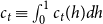 $ c_{t}\equiv \int _{0}^{1}c_{t} ( h ) dh$
. Therefore, due to the homothetic preference, the growth rate of consumption is uniform across all households.
3.2 Final good and labor unions
A representative firm produces final good
 $Y_{t}$
using the following production function:
 \begin{equation} Y_{t}=\int _{0}^{N_{t}}X_{t}^{\theta }\left ( i\right ) \left [ Z_{t}^{\alpha }\left ( i\right ) Z_{t}^{1-\alpha }\left ( \frac {l_{t}}{N_{t}}\right ) ^{\eta } \right ] ^{1-\theta }di, \end{equation}
where
 $\left \{ \theta ,\alpha ,\eta \right \} \in \left ( 0,1\right )$
. The mass of differentiated non-durable intermediate goods at time
 $t$
is
 $N_{t}$
, and
 $X_{t}\left ( i\right )$
denotes the quantity of intermediate good
 $ i\in \left [ 0,N_{t}\right ]$
. The productivity of each intermediate good
 $i$
is determined by its quality
 $Z_{t}\left ( i\right )$
and by the average quality of all intermediate goods
 $Z_{t}\equiv \big [ \int _{0}^{N_{t}}Z_{t} ( i )\, di\big ] /N_{t}$
which captures technology spillovers across firms. Aggregate employment is
 $l_{t}$
, and the term
 $l_{t}/N_{t}$
implies that technology features a congestion effect of variety, which removes the scale effect of labor size on long-run growth. The final-good production technology features decreasing returns to scale
 $\eta \lt 1$
, ensuring that the representative final-good firm earns positive profits. This assumption facilitates bargaining between employers and labor unions and can be justified by the presence of fixed factors such as entrepreneurial skills possessed by the firm owner.
The profit function of the final-good firm is
 \begin{equation} \Pi _{t}=Y_{t}-w_{t}l_{t}-\int _{0}^{N_{t}}p_{t}\left ( i\right ) X_{t}\left ( i\right ) di, \end{equation}
where
 $p_{t}\left ( i\right )$
is the price of intermediate good
 $i$
, and the price of final good is normalized to one. Profit maximization yields the conditional demand function for
 $X_{t}\left ( i\right )$
:
 \begin{equation} X_{t}\left ( i\right ) =\left [ \frac {\theta }{p_{t}\left ( i\right ) }\right ] ^{1/\left ( 1-\theta \right ) }Z_{t}^{\alpha }\left ( i\right ) Z_{t}^{1-\alpha }\left ( \frac {l_{t}}{N_{t}}\right ) ^{\eta}\!. \end{equation}
Therefore, the final-good firm pays
 $\theta Y_{t}=\int _{0}^{N_{t}}p_{t}\left ( i\right ) X_{t}\left ( i\right ) di$
for intermediate goods.
The asset-pricing equation for the final-good firm is
 \begin{equation} r_{t}=\frac {\Pi _{t}}{v_{t}}+\frac {\dot {\!v}_{t}}{v_{t}}, \end{equation}
where
 $v_{t}$
represents the market value of the final-good firm. This equation states that the return on equity shares is determined by profit flow and capital gains.
Following the modeling approach of Pemberton (Reference Pemberton1988), we consider a managerial labor union whose objective is determined by both the union leaders’ preference for a larger membership (employment level) and the union members’ preference for a higher wage. The objective function of the labor union is given by the following Stone-Geary utility function:
 \begin{equation} O_{t}=( w_{t}-b_{t}) ^{\omega }l_{t}. \end{equation}
The parameter
 $\omega \gt 0$
determines the relative importance of wage income net of unemployment benefit
 $w_{t}-b_{t}$
in the union’s objective function. The union is wage-oriented when
 $\omega \gt 1$
, and employment-oriented when
 $ \omega \lt 1$
. In the remainder of the paper, we focus on the empirically relevant case of a wage-oriented union (
 $\omega \gt 1$
), while the employment-oriented case (
 $\omega \lt 1$
) is analyzed in Appendix C.
The labor union bargains with the employer federation to determine the equilibrium wage
 $w_{t}$
and employment level
 $l_{t}$
. The generalized Nash bargaining function is
 \begin{equation} \underset {w_{t},l_{t}}{\max }B_{t}=O_{t}^{\gamma }\Pi _{t}^{1-\gamma }=\left [ \left ( w_{t}-b_{t}\right ) ^{\omega }l_{t}\right ] ^{\gamma }\left [ Y_{t}-w_{t}l_{t}-\int _{0}^{N_{t}}p_{t}\left ( i\right ) X_{t}\left ( i\right ) di \right ] ^{1-\gamma}\!. \end{equation}
The parameter
 $\gamma \in \left ( 0,1\right )$
represents the bargaining power of the labor union, while
 $1-\gamma$
represents the bargaining power of the employer. The first-order conditions for the Nash bargaining solutions are
 \begin{equation} \frac {\partial B_{t}}{\partial w_{t}}=0\Rightarrow \frac {( w_{t}-b_{t}) l_{t}}{\Pi _{t}}=\frac {\omega \gamma }{1-\gamma }, \end{equation}
 \begin{equation} \frac {\partial B_{t}}{\partial l_{t}}=0\Rightarrow \frac {w_{t}l_{t}-\eta \left ( 1-\theta \right ) Y_{t}}{\Pi _{t}}=\frac {\gamma }{1-\gamma }. \end{equation}
Equations (10) and (11) jointly determine the equilibrium employment
 $l_{t}$
and the Pareto-optimal allocation between labor income
 $w_{t}l_{t}$
and firm profit
 $\Pi _{t}$
.
3.3 Intermediate goods and in-house R&D
The market structure of the intermediate goods sector is monopolistic competition, where each firm produces one type of differentiated intermediate good. A monopolistic firm uses
 $X_{t}\left ( i\right )$
units of final goods to produce
 $X_{t}\left ( i\right )$
units of intermediate goods for
 $i\in \left [ 0,N_{t}\right ]$
, such that the marginal cost of production is equal to one. The firm also incurs a fixed operating cost of
 $\phi Z_{t}^{\alpha }\left ( i\right ) Z_{t}^{1-\alpha }$
units of final goods. Additionally, the firm invests
 $R_{t}\left ( i\right )$
units of final goods in in-house R&D to improve the quality of its product with the following innovation process:
 \begin{equation} \dot {\!Z}_{t}\left ( i\right ) =R_{t}\left ( i\right ). \end{equation}
The firm’s profit flow before-R&D at time
 $t$
is expressed as
 \begin{equation} \pi _{t}\left ( i\right ) =[ p_{t}\left ( i\right ) -1] X_{t}\left ( i\right ) -\phi Z_{t}^{\alpha }\left ( i\right ) Z_{t}^{1-\alpha }. \end{equation}
The market value of the firm is
 \begin{equation} V_{t}\left ( i\right ) =\int _{t}^{\infty }\exp \left ( -\int _{t}^{s}r_{v}dv\right ) \left [ \pi _{s}\left ( i\right ) -R_{s}\left ( i\right ) \right ] ds. \end{equation}
The firm maximizes its value equation (14) subject to the demand function equation (6), the innovation process equation (12), and the profit function equation (13). The unconstrained profit-maximizing price is
 $p_{t}\left ( i\right ) =1/\theta$
(see Appendix A). Following Chu et al. (Reference Chu, Kou and Wang2020, Reference Chu, Furukawa, Mallick, Peretto and Wang2021), knowledge diffuses from the monopolistic firm to imitators in each industry
 $i\in \left [ 0,N_{t}\right ]$
. However, imitative firms can only produce good
 $i$
at a higher marginal cost
 $\mu \in \left ( 1,1/\theta \right )$
with the same quality as the monopolistic firm due to the legal regulations such as patent laws. Therefore, the monopolistic firm sets its price at
 $p_{t}\left ( i\right ) =\mu$
to price out imitators from the market.
The initial quality of differentiated goods is identical across firms, with
 $ Z_{0}\left ( i\right ) =Z_{0}$
for
 $i\in \left [ 0,N_{0}\right ]$
, which implies that symmetric equilibrium holds at any point in time across all industries, such that
 $Z_{t}\left ( i\right ) =Z_{t}$
and
 $X_{t}\left ( i\right ) =X_{t}$
, and consequently
 $\pi _{t}\left ( i\right ) =\pi _{t}$
,
 $ R_{t}\left ( i\right ) =R_{t}$
, and
 ${V_{t}\left ( i\right ) =V_{t}}$
. By substituting
 $p_{t}\left ( i\right ) =\mu$
into the demand function equation (6) and imposing symmetry, the quality-adjusted firm size is derived as
 \begin{equation*} \frac {X_{t}}{Z_{t}}=\left ( \frac {\theta }{\mu }\right ) ^{1/\left ( 1-\theta \right ) }\left ( \frac {l_{t}}{N_{t}}\right ) ^{\eta}\!, \end{equation*}
which is determined by
 $l_{t}/N_{t}$
. For analytical convenience, we define the following state variable:
 \begin{equation} x_{t}\equiv \frac {\mu ^{1/\left ( 1-\theta \right ) }}{l_{t}^{\eta }}\frac { X_{t}}{Z_{t}}=\frac {\theta ^{1/\left ( 1-\theta \right ) }}{N_{t}^{\eta }} , \end{equation}
which is determined by the quality-adjusted firm size
 $X_{t}/Z_{t}$
. A change in the bargaining power of labor unions
 $\gamma$
does not directly affect
 $x_{t}$
through the market size
 $l_{t}$
, but indirectly through the number of products
 $N_{t}$
. In Appendix A, we derive the rate of return to quality-improving R&D
 $r_{t}^{q}$
given by
 \begin{equation} r_{t}^{q}=\alpha \frac {\pi _{t}}{Z_{t}}=\alpha \left [ \frac {\mu -1}{\mu ^{1/\left ( 1-\theta \right ) }}x_{t}l_{t}^{\eta }-\phi \right ]\!, \end{equation}
which is increasing in both
 $x_{t}$
and
 $l_{t}$
.
3.4 Entrants
A new firm incurs an entry cost of
 $\beta X_{t}$
(where
 $\beta \gt 0$
) units of final goods to invent a new variety of intermediate goods with quality
 $ Z_{t}$
, ensuring symmetric equilibrium holds at any point in time. This specification of the entry cost implies that the setup cost for an entrant increases with the size of its initial output. The rate of return on assets is determined by its profit flow net of in-house R&D and the capital gain in firm value. The asset-pricing equation is
 \begin{equation} r_{t}=\frac {\pi _{t}-R_{t}}{V_{t}}+\frac {\dot {\!V}_{t}}{V_{t}}. \end{equation}
The free-entry condition is
 \begin{equation} V_{t}=\beta X_{t}. \end{equation}
Substituting equations (12), (13), (15), (18), and
 $p_{t}\left ( i\right ) =\mu$
into the asset-pricing equation (17) yields the return to entry as
 \begin{equation} r_{t}^{e}=\frac {\mu ^{1/\left ( 1-\theta \right ) }}{\beta }\left [ \frac {\mu -1 }{\mu ^{1/\left ( 1-\theta \right ) }}-\frac {\phi +z_{t}}{x_{t}l_{t}^{\eta }} \right ] +\frac {\dot {\!x}_{t}}{x_{t}}+z_{t}+\eta \frac {\dot {\!l}_{t}}{l_{t}}, \end{equation}
where
 $z_{t}\equiv \dot {\!Z}_{t}/Z_{t}$
is the growth rate of aggregate quality. The scrap value of exiting an industry is equal to the entry cost
 $ \beta X_{t}$
, such that
 $V_{t}\left ( i\right ) =\beta X_{t}$
always holds, which implies that
 $r_{t}^{e}=r_{t}$
at any point in time.
3.5 Government
The government provides unemployment benefits to households and levies a lump-sum tax on households to finance the benefits. The balanced-budget condition for the government is
 \begin{equation} \tau _{t}=b_{t}\left ( L-l_{t}\right )\!. \end{equation}
Assume that unemployment benefit
 $b_{t}$
is proportional to output
 $Y_{t}$
, such that
 $b_{t}=\bar {b}Y_{t}$
with
 $\bar {b}\gt 0$
, ensuring balanced growth. The lump-sum tax
 $\tau _{t} ( h )$
levied on household
 $h$
is given by
 $\tau _{t} ( h ) =b_{t} [ L-l_{t} ( h ) ]$
. This setup eliminates the effects of lump-sum taxes and unemployment benefits on inequality.
3.6 General equilibrium
The general equilibrium is a time path of allocations
 $ \{a_{t},c_{t},Y_{t},l_{t},X_{t}\left ( i\right ) ,R_{t}\left ( i\right ) \}$
, prices
 $\{r_{t},w_{t},$
 $p_{t}\left ( i\right ) ,v_{t},V_{t}\left ( i\right ) \}$
, and government policies
 $\{\tau _{t},b_{t}\}$
such that the following conditions hold:
-
• households choose
 $c_{t} ( h )$
to maximize their lifetime utility, taking
$\{r_{t},w_{t},b_{t},\tau _{t} ( h ) \}$
as given;
-
• the representative final-good firm produces
$Y_{t}$
to maximize its profit, taking
$p_{t} ( i )$
as given; -
• a representative employer of final-good firm bargains with a representative labor union to determine
$\{w_{t},l_{t}\}$
; -
• monopolistic firms produce intermediate goods
$X_{t} ( i )$
and choose
$\{p_{t} ( i ) ,R_{t} ( i ) \}$
to maximize their market value
$V_{t} ( i )$
, taking
$r_{t}$
as given; -
• entrants make entry decisions, taking
$V_{t}$
as given; -
• the sum of the value of the representative final-good firm and the value of all existing monopolistic firms is equal to the value of households’ financial assets:
$v_{t}+N_{t}V_{t}=\int _{0}^{1}a_{t} ( h ) dh\equiv a_{t}$
; -
• the government balances its budget such that
$\tau _{t}=b_{t} ( L-l_{t} )$
; -
• the market-clearing condition for labor holds such that
$ \int _{0}^{1}l_{t} ( h) dh=l_{t}$
; and -
• the market-clearing condition for final good holds such that
$ Y_{t}=c_{t}+N_{t} ( X_{t}+\phi Z_{t}+R_{t} ) +$
$\dot {\!N}_{t}\beta X_{t}$
.









3.6.1 Equilibrium employment
Substituting the profit of the final-good firm
 $\Pi _{t}=\left ( 1-\theta \right ) Y_{t}-w_{t}l_{t}$
into equation (11) yields the labor share:
 \begin{equation} \frac {w_{t}l_{t}}{Y_{t}}=\left ( 1-\theta \right ) \left [ \eta +\left ( 1-\eta \right ) \gamma \right ]\!, \end{equation}
which is increasing in the bargaining power of the labor union
 $\gamma$
. Substituting this expression into the profit function
 $\Pi _{t}$
yields the profit of the final-good firm as a share of final output:
 \begin{equation} \frac {\Pi _{t}}{Y_{t}}=\left ( 1-\theta \right ) \left ( 1-\eta \right ) \left ( 1-\gamma \right )\!, \end{equation}
which is decreasing in
 $\gamma$
. Substituting equations (21), (22) and
 $b_{t}=\bar {b}Y_{t}$
into equation (10) yields the equilibrium level of employment:Footnote
2
 \begin{equation} l_{t}=\left ( 1-\theta \right ) \frac {\eta +\left ( 1-\eta \right ) \left ( 1-\omega \right ) \gamma }{\bar {b}}\equiv l\lt L, \end{equation}
which is decreasing in the wage orientation of the labor union
 $\omega$
. When the labor union is wage-oriented
 $\omega \gt 1$
, the equilibrium level of employment
 $l$
is decreasing in its bargaining power
 $\gamma$
. We summarize these results in Lemma1.
Lemma 1.
Labor share is increasing in the union bargaining power
 $\gamma$
, and the profit share of the final-good firm is decreasing in
 $\gamma$
. Employment is decreasing in
 $\gamma$
for a wage-oriented labor union
 $\omega \gt 1$
.
Proof. Proven in text.
3.6.2 Aggregation
Substituting the demand for
 $X_{t}\left ( i\right )$
in equation (6) and
 $ p_{t}\left ( i\right ) =\mu$
into the final-good production function in equation (4) and imposing symmetry yields the aggregate final-good production function as
 \begin{equation} Y_{t}=\left ( \theta /\mu \right ) ^{\theta /\left ( 1-\theta \right ) }N_{t}^{1-\eta }Z_{t}l^{\eta}. \end{equation}
The growth rate of output is
 \begin{equation} g_{t}\equiv \frac {\dot {\!Y}_{t}}{Y_{t}}=\left ( 1-\eta \right ) n_{t}+z_{t}, \end{equation}
where
 $n_{t}\equiv \dot {\!N}_{t}/N_{t}$
is the variety growth rate and
 $z_{t}$
is the quality growth rate.
4. Dynamics
This section analyzes the dynamic properties of the model. Section 4.1analyzes the dynamics of the aggregate economy, including the dynamic paths of
 $x_{t}$
and
 $g_{t}$
. Section 4.2 investigates the dynamics of the wealth distribution, while Section 4.3 explores the dynamics of the income distribution. Finally, Section 4.4 studies the dynamics of the consumption distribution.
4.1 Dynamics of the aggregate economy
In this model, the dynamics of
 $x_{t}$
determines the dynamics of the economy. To analyze the transition dynamics of
 $x_{t}$
and
 $g_{t}$
, we first show an important property of the model: the consumption-output ratio
 $ c_{t}/Y_{t}$
and the consumption-wealth ratio
 $c_{t}/a_{t}$
remain constant along both the transition path and the balanced-growth path. Define the parameter
 $\Theta \equiv \beta \theta /\left [ \mu \left ( 1-\theta \right ) \right ]$
.
Lemma 2. The consumption-output ratio jumps to its stable steady-state value:
 \begin{equation} \frac {c_{t}}{Y_{t}}=(1-\theta )(1+\rho \Theta ). \end{equation}
The consumption-wealth ratio also jumps to its stable steady-state value:
 \begin{equation} \frac {c_{t}}{a_{t}}=\frac {\rho (1+\rho \Theta )}{\rho \Theta +\left ( 1-\eta \right ) \left ( 1-\gamma \right ) }. \end{equation}
Proof. See Appendix A.
The stationarity of the consumption-output ratio
 $c_{t}/Y_{t}$
implies that consumption and output grow at the same rate at any time
 $t$
. Therefore, from the Euler equation in equation (3), the growth rate of output is given by
 \begin{equation*} g_{t}\equiv \frac {\dot {\!Y}_{t}}{Y_{t}}=\frac {\dot {\!c}_{t}}{c_{t}}=r_{t}-\rho , \end{equation*}
and substituting
 $r_{t}^{q}$
in equation (16) into it yields the growth rate of output as
 \begin{equation} g_{t}=\alpha \left [ \frac {\mu -1}{\mu ^{1/\left ( 1-\theta \right ) }} x_{t}l^{\eta }-\phi \right ] -\rho , \end{equation}
which is increasing in the quality-adjusted firm size
 $x_{t}l^{\eta }$
. The growth rate of output
 $g_{t}$
is positive if and only if:
 \begin{equation*} x_{t}\gt \bar {\!x}\equiv \frac {\mu ^{1/\left ( 1-\theta \right ) }}{\left ( \mu -1\right ) l^{\eta }}\left ( \frac {\rho }{\alpha }+\phi \right )\!. \end{equation*}
Since the market size of each intermediate good determines profit and R&D incentives, firm size must be large enough to provide sufficient incentives for innovation. For the rest of the paper, we assume that
 $x_{t}\gt \bar {x}$
always holds. The dynamics of
 $x_{t}$
are summarized in the Proposition1.
Proposition 1.
The dynamics of
 $x_{t}$
follows the linearized autonomous differential equation:
 \begin{equation} \dot {\!x}_{t}=\frac {\eta }{\beta }\mu ^{1/\left ( 1-\theta \right ) }\left [ \frac {\left ( 1-\alpha \right ) \phi -\rho }{l^{\eta }}\right ] -\frac {\eta }{ \beta }\left [ \left ( 1-\alpha \right ) \left ( \mu -1\right ) -\beta \rho \right ] x_{t}. \end{equation}
Under the parameter restriction
 $\rho \lt \min \left \{ \left ( 1-\alpha \right ) \phi ,\left ( 1-\alpha \right ) \left ( \mu -1\right ) /\beta \right \}$
,
 $x_{t}$
is globally stable and gradually converges to its steady-state value:
 \begin{equation} x^{\ast }=\frac {\mu ^{1/\left ( 1-\theta \right ) }}{l^{\eta }}\frac {\left ( 1-\alpha \right ) \phi -\rho }{\left ( 1-\alpha \right ) \left ( \mu -1\right ) -\beta \rho }\gt \bar {x}. \end{equation}
The steady-state growth rate of output is
 \begin{equation} g^{\ast }=\alpha \left [ \left ( \mu -1\right ) \frac {\left ( 1-\alpha \right ) \phi -\rho }{\left ( 1-\alpha \right ) \left ( \mu -1\right ) -\beta \rho }-\phi \right ] -\rho \gt 0. \end{equation}
Proof. See Appendix A.
The dynamic paths of
 $x_{t}$
and
 $g_{t}$
can be illustrated as follows. Given an initial value
 $x_{0}\lt$
 $x^{\ast }$
(
 $\gt$
 $x^{\ast }$
),
 $x_{t}$
rises (declines) gradually and converges to its steady-state value
 $x^{\ast }$
along the path described by
 $\dot {\!x}_{t}$
. The output growth rate
 $g_{t}$
rises (declines) gradually and converges to its steady-state value
 $g^{\ast }$
. The number of differentiated products
 $N_{t}$
adjusts according to
 $ N_{t}=[\theta ^{1/(1-\theta )}/x_{t}]^{1/\eta }$
. Over time,
 $N_{t}$
declines (rises) and converges to its steady-state value
 $N^{\ast }=(\theta ^{1/(1-\theta )}/x^{\ast })^{1/\eta }$
.
4.2 Dynamics of the wealth distribution
From the Euler equation in equation (3), all households share the same consumption growth rate
 $\,\dot {\!c}_{t} ( h ) /c_{t} ( h ) = \dot {\!c}_{t}/c_{t}=r_{t}-\rho$
. This implies that the consumption share of each household, defined as
 $s_{c,t} ( h ) \equiv c_{t} ( h ) /c_{t}$
, remains constant and is equal to its initial value
 $ s_{c,0} ( h ) =c_{0} ( h ) /c_{0}$
for
 $h\in \left [ 0,1 \right ]$
, which is endogenously determined, as shown in the Proof of Proposition2.
The wealth share of household
 $h$
is defined as
 $s_{a,t} ( h ) \equiv a_{t} ( h ) /a_{t}$
, and its initial value
 $s_{a,0} ( h ) =a_{0} ( h ) /a_{0}$
is exogenously given at time 0. The growth rate of the wealth share
 $s_{a,t} ( h )$
is given byFootnote
3
 \begin{equation*} \frac {\dot {\!s}_{a,t} ( h ) }{s_{a,t} ( h ) }=\frac {\dot {\!a} _{t} ( h ) }{a_{t} ( h ) }-\frac {\dot {\!a}_{t}}{a_{t}}=\frac { c_{t}-w_{t}l_{t}}{a_{t}}-\frac {s_{c,t} ( h ) c_{t}-w_{t}l_{t}}{ a_{t} ( h ) }. \end{equation*}
Proposition2 shows that the wealth distribution among households remains stationary and is determined by its initial distribution such that
 $ s_{a,t} ( h ) =s_{a,0} ( h )$
. In the Proof of Proposition2, we derive the dynamics of
 $s_{a,t} ( h )$
featured by the following one-dimensional linear differential equation:
 \begin{equation*} \dot {\!s}_{a,t} ( h ) =\rho s_{a,t} ( h ) -\frac {c_{t}}{a_{t} }\left [ s_{c,t} ( h ) -\frac {w_{t}l_{t}}{c_{t}}\right ]\!. \end{equation*}
We show that for any
 $t\geq 0$
, the condition
 $\dot {\!s}_{a,t} ( h ) =0$
must hold, and
 $s_{c,t} ( h )$
must immediately jump to its steady-state value at
 $t=0$
such that
 $s_{c,t} ( h ) =s_{c,0} ( h )$
. This ensures the stability of
 $s_{a,t} ( h )$
, resulting in a constant wealth share of household
 $h\in \left [ 0,1\right ]$
. The stationarity of wealth distribution along both the transition and balanced-growth paths arises from the stationary consumption-output ratio
 $ c_{t}/Y_{t}$
and consumption-wealth ratio
 $c_{t}/a_{t}$
, despite the transition dynamics of the aggregate economy, which is governed by the law of motion of
 $x_{t}$
.
Proposition 2.
The wealth share
 $s_{a,t} ( h )$
of household
 $ h\in \left [ 0,1\right ]$
remains constant and is equal to its initial value at
 $t=0$
such that
 \begin{equation} s_{a,t} ( h ) =s_{a,0} ( h ) . \end{equation}
Therefore, the wealth distribution is stationary along both the transition and balanced-growth paths.
Proof. See Appendix A.
We derive the Gini coefficient of wealth following Chu and Peretto (Reference Chu and Peretto2023). We rank households
 $h\in \left [ 0,1\right ]$
in ascending order of wealth, and define the Gini coefficient of wealth at time
 $t$
as
 \begin{equation*} \sigma _{a,t}^{G}\equiv 1-2\int _{0}^{1}\mathcal{L} _{a,t} ( h ) dh , \end{equation*}
where the Lorenz curve of wealth is given by
 \begin{equation*} \mathcal{L} _{a,t} ( h ) \equiv \frac {\int _{0}^{h}a_{t}\left ( \chi \right ) d\chi }{\int _{0}^{1}a_{t}\left ( \chi \right ) d\chi }=\frac { \int _{0}^{h}a_{t}\left ( \chi \right ) d\chi }{a_{t}}=\int _{0}^{h}s_{a,t} \left ( \chi \right ) d\chi =\int _{0}^{h}s_{a,0}\left ( \chi \right ) d\chi . \end{equation*}
Since the Lorenz curve of wealth remains unchanged over time,
 $\mathcal{L} _{a,t} ( h ) =\mathcal{L} _{a,0} ( h ) =\mathcal{L} _{a} ( h )$
, the Gini coefficient of wealth remains constant
 $ \sigma _{a,t}^{G}=\sigma _{a,0}^{G}=\sigma _{a}^{G}$
for all time, where
 $ \sigma _{a,0}^{G}$
is the Gini coefficient of wealth at
 $t=0$
.
4.3 Dynamics of the income distribution
The income distribution features transition dynamics and is determined by both the unequal distribution of wealth and the ratio of asset income to labor income
 $r_{t}a_{t}/w_{t}l_{t}$
. The evolution of income distribution is determined by the transition dynamics of the aggregate economy, specifically, the transition dynamics of the output growth rate
 $g_{t}$
, which in turn determines the real interest rate
 $r_{t}$
.
The total income received by household
 $h$
consists of its asset income and wage income given byFootnote
4
 \begin{equation*} I_{t} ( h ) =r_{t}a_{t} ( h ) +w_{t}l_{t}. \end{equation*}
Aggregating across all households
 $h\in \left [ 0,1\right ]$
, the aggregate income of the economy is given by
 \begin{equation*} I_{t}=r_{t}a_{t}+w_{t}l_{t}. \end{equation*}
The income share of household
 $h$
is defined as
 $s_{I,t} ( h ) \equiv I_{t} ( h ) /I_{t}$
, which, using
 $s_{a,t} ( h ) =s_{a,0} ( h )$
, can be expressed as
 \begin{equation} s_{I,t} ( h ) =\frac {r_{t}a_{t} ( h ) +w_{t}l_{t}}{ r_{t}a_{t}+w_{t}l_{t}}=\frac {r_{t}a_{t}}{r_{t}a_{t}+w_{t}l_{t}}s_{a,0} ( h ) +\frac {w_{t}l_{t}}{r_{t}a_{t}+w_{t}l_{t}}, \end{equation}
Equation (33) shows that the income share of each household consists of two components, the labor income share which is identical across all households and equal to the aggregate labor income share, and the asset income share which varies across households and is determined by the wealth share they hold. If household
 $h$
’s wealth share
 $s_{a,t} ( h )$
is larger than one (the average wealth share), an increase in the aggregate asset income share leads to an increase in its income share
 $s_{I,t} ( h )$
. Conversely, if household
 $h$
’s wealth share is smaller than one, an increase in the aggregate asset income share leads to a decrease in its income share.
We derive the Gini coefficient of income and the top income share. Households are sorted in ascending order of income, and the Gini coefficient of income at time
 $t$
is given by
 \begin{equation} \sigma _{I,t}^{G}=\frac {r_{t}a_{t}}{r_{t}a_{t}+w_{t}l_{t}}\sigma _{a}^{G} . \end{equation}
Equation (34) shows that income inequality
 $\sigma _{I,t}^{G}$
is lower than wealth inequality
 $\sigma _{a}^{G}$
because labor income is identical across all households. Income inequality
 $\sigma _{I,t}^{G}$
in this model is driven by wealth inequality
 $\sigma _{a}^{G}$
, and it increases with the asset-to-wage income ratio
 $r_{t}a_{t}/\left ( w_{t}l_{t}\right )$
. Proposition3 provides the analytical expression for the Gini coefficient of income
 $\sigma _{I,t}^{G}$
, which features transition dynamics and is increasing in the output growth rate
 $g_{t}$
, as a higher growth rate increases the real interest rate
 $r_{t}$
through the Euler equation.
The coefficient of variation of income is
 \begin{equation*} \sigma _{I,t}\equiv \sqrt {\int _{0}^{1}\left [ s_{I,t} ( h ) -1\right ] ^{2}dh}=\frac {r_{t}a_{t}}{r_{t}a_{t}+w_{t}l_{t}}\sigma _{a}, \end{equation*}
where the coefficient of variation of wealth is defined as
 $\sigma _{a}\equiv \sqrt {\int _{0}^{1}\left [ s_{a,0} ( h ) -1\right ] ^{2}dh}$
.
Proposition 3.
The degree of income inequality, measured by the Gini coefficient of income at any time
 $t$
is given by
 \begin{equation} \sigma _{I,t}^{G}=\left [ 1+\frac {\rho }{\rho +g_{t}}\frac {\gamma +\eta /\left ( 1-\eta \right ) }{1+\rho \Theta /\left ( 1-\eta \right ) -\gamma } \right ] ^{-1}\sigma _{a}^{G}. \end{equation}
Proof. See Appendix A.
The share of total income owned by the top
 $\varepsilon$
households is given by
 \begin{equation} s_{I,t}^{\varepsilon }\equiv \int _{1-\varepsilon }^{1}s_{I,t} ( h ) dh=\frac {r_{t}a_{t}}{r_{t}a_{t}+w_{t}l_{t}}\int _{1-\varepsilon }^{1}s_{a,0} ( h ) dh+\frac {w_{t}l_{t}}{r_{t}a_{t}+w_{t}l_{t}} \varepsilon =\frac {\sigma _{I,t}^{G}}{\sigma _{a}^{G}}\left ( s_{a,0}^{\varepsilon }-\varepsilon \right ) +\varepsilon , \end{equation}
which uses equation (34) and the wealth share held by the top
 $ \varepsilon$
households denoted by
 $s_{a,0}^{\varepsilon }=\int _{1-\varepsilon }^{1}s_{a,0} ( h ) dh$
. Equation (36) indicates that the income share of the top
 $\varepsilon$
households
 $s_{I,t}^{\varepsilon }$
is increasing in the Gini coefficient of income
 $\sigma _{I,t}^{G}$
if and only if the top
 $\varepsilon$
households hold a wealth share greater than
 $\varepsilon$
, i.e.,
 $s_{a,0}^{\varepsilon }\gt \varepsilon$
. Since the Gini coefficient of wealth
 $\sigma _{a}^{G}$
is stationary, changes in income inequality arise solely from the evolution of the asset-to-wage income ratio
 $r_{t}a_{t}/ ( w_{t}l_{t} )$
.
4.4 Dynamics of the consumption distribution
The household
 $h$
’s consumption is given by
 \begin{equation*} c_{t} ( h ) =\left [ r_{t}-\frac {\dot {\!a}_{t} ( h ) }{ a_{t} ( h ) }\right ] a_{t} ( h ) +w_{t}l_{t} ( h ) =\rho a_{t} ( h ) +w_{t}l_{t}, \end{equation*}
where we have used the Euler equation in equation (3),
 $b_{t} [ L-l_{t} ( h ) ] =\tau _{t} ( h )$
,
 $l_{t} ( h ) =l_{t}$
, and
 $\dot {\!a}_{t} ( h ) /a_{t} ( h ) =\dot {\! a}_{t}/a_{t}=\dot {\!c}_{t}/c_{t}$
. This equation indicates that household consumption consists of labor income
 $w_{t}l_{t}$
and a constant fraction
 $ \rho$
of wealth
 $a_{t} ( h )$
. Aggregating across all households yields the aggregate consumption given by
 \begin{equation*} c_{t}=\int _{0}^{1}c_{t} ( h ) dh=\rho a_{t}+w_{t}l_{t}. \end{equation*}
The share of consumption owned by household
 $h$
at time
 $t$
is
 \begin{equation} s_{c,t} ( h ) =\frac {\rho a_{t} ( h ) +w_{t}l_{t}}{\rho a_{t}+w_{t}l_{t}}=\frac {\rho a_{t}}{\rho a_{t}+w_{t}l_{t}}s_{a,0} ( h ) +\frac {w_{t}l_{t}}{\rho a_{t}+w_{t}l_{t}}. \end{equation}
The Gini coefficient of consumption is given by
 \begin{equation} \sigma _{c,t}^{G}=\frac {\rho a_{t}}{\rho a_{t}+w_{t}l_{t}}\sigma _{a}^{G} , \end{equation}
which can also be expressed as (see Appendix A)
 \begin{equation} \sigma _{c,t}^{G}=\left [ 1+\frac {\gamma +\eta /\left ( 1-\eta \right ) }{ 1+\rho \Theta /\left ( 1-\eta \right ) -\gamma }\right ] ^{-1}\sigma _{a}^{G} . \end{equation}
Equation (38) shows that consumption inequality is stationary
 $\sigma _{c,t}^{G}=\sigma _{c,0}^{G}$
and is lower than wealth inequality
 $\sigma _{a}^{G}$
. Furthermore, comparing equations (35) and (39), we see that consumption inequality
 $\sigma _{c,t}^{G}$
is lower than income inequality
 $\sigma _{I,t}^{G}$
if and only if the growth rate
 $g_{t}$
is positive.
The consumption share of the top
 $\varepsilon$
households is
 \begin{equation} s_{c,t}^{\varepsilon }\equiv \int _{1-\varepsilon }^{1}s_{c,t} ( h ) dh=\frac {\rho a_{t}}{\rho a_{t}+w_{t}l_{t}}\int _{1-\varepsilon }^{1}s_{a,0} ( h ) dh+\frac {w_{t}l_{t}}{\rho a_{t}+w_{t}l_{t}} \varepsilon =\frac {\sigma _{c,t}^{G}}{\sigma _{a}^{G}}\left ( s_{a,0}^{\varepsilon }-\varepsilon \right ) +\varepsilon , \end{equation}
which uses equation (38). Equation (36) states that the consumption share of the top
 $\varepsilon$
households
 $ s_{c,t}^{\varepsilon }$
is increasing in the Gini coefficient of consumption
 $\sigma _{c,t}^{G}$
if and only if the wealth share of the top
 $\varepsilon$
households is larger than
 $\varepsilon$
, i.e.,
 $s_{a,0}^{\varepsilon }\gt \varepsilon$
. Since the Gini coefficient of wealth
 $\sigma _{a}^{G}$
is stationary, the only source of change in consumption inequality is the evolution of the asset-to-wage income ratio
 $r_{t}a_{t}/ ( w_{t}l_{t} )$
.
5. Dynamic effects of labor unions
This section explores the dynamic effects of union bargaining power on economic growth, income inequality, and social welfare analytically and quantitatively. Section 5.1 presents the analytical results. Section 5.2 presents the quantitative results. Section 5.3 performs a welfare analysis.
5.1 Analytical results
We analyze the effects of stronger bargaining power of a wage-oriented labor union
 $\gamma$
on growth and inequality. Equations (23) and (28) show that an increase in union bargaining power
 $\gamma$
initially reduces the growth rate of output
 $g_{t}$
. Equation (23) shows that stronger union bargaining power, a larger
 $\gamma$
, leads to a permanent decline in employment
 $l$
. This negative market-size effect reduces the incentives for monopolistic firms to do in-house R&D
 $r_{t}^{q}$
, which reduces the growth rates of quality
 $z_{t}$
and output
 $g_{t}$
in the short run. However, the market structure is endogenous and the number of firms adjusts gradually. The smaller market size forces some firms to exit the market, which subsequently increases the firm size
 $x_{t}l^{\eta }$
and the rate of return on quality-improving innovation
 $r_{t}^{q}$
. In the long run, the positive entry effect offsets the negative market-size effect such that the steady-state growth rate returns to its initial value because
 $ g^{\ast }$
is independent of
 $\gamma$
. In summary, the endogenous market structure gives rise to distinct effects of
 $\gamma$
on
 $g_{t}$
at different time horizons; see Figure 6 for an illustration in which
 $\gamma$
increases at time
 $t$
.
The effect of union bargaining power on income inequality is determined by both the rate of return on assets
 $r_{t}$
and the asset-to-wage income ratio
 $a_{t}/w_{t}l_{t}$
. Equation (35) shows that an increase in
 $ \gamma$
reduces income inequality
 $\sigma _{I,t}^{G}$
in the short run. The short-run effect operates through two channels. A negative interest-rate effect arises because a larger
 $\gamma$
lowers the growth rate
 $g_{t}$
, which in turn reduces the real interest rate
 $r_{t}$
via the Euler equation. There is also a negative income-share effect, captured by
 $a_{t}/w_{t}l_{t}$
, which arises because a larger
 $\gamma$
increases the labor income share and reduces the profit share and the ratio of assets to output
 $a_{t}/Y_{t}$
. Since both effects work in the same direction, the short-run effect of a larger
 $\gamma$
on
 $\sigma _{I,t}^{G}$
is negative. In the long run, the interest-rate effect vanishes due to the endogenous market structure, leading to a scale-invariant steady-state growth rate
 $g^{\ast }$
and real interest rate
 $r^{\ast }$
. However, the negative income-share effect persists, implying that an increase in union bargaining power results in a permanent reduction in income inequality
 $(\sigma _{I}^{G})^{\ast }$
; see Figure 7.
Dynamic effects of labor unions on economic growth (
 $ \omega \gt 1$
).

Equation (39) shows that a larger
 $\gamma$
results in a one-time permanent decrease in consumption inequality
 $\sigma _{c,t}^{G}$
(see Figure 8), which is caused by the negative income-share effect, captured by
 $\rho a_{t}/w_{t}l_{t}$
. Unlike the effect on income inequality, the interest-rate effect is absent because the log utility function ensures that consumption distribution remains stationary. Proposition4 summarizes the above results. See Appendix C for the analysis of an employment-oriented union (
 $\omega \lt 1$
).
Proposition 4. A stronger bargaining power of a wage-oriented labor union has the following effects on economic growth and inequality: (a) it reduces economic growth and income inequality in the short run; (b) it reduces income inequality but does not affect the steady-state growth rate in the long run; and (c) it causes a one-time permanent reduction in consumption inequality.
Proof. Proven in text.
Dynamic effects of labor unions on income inequality (
 $ \omega \gt 1$
).

Dynamic effects of labor unions on consumption inequality.

5.2 Quantitative analysis
In this section, we calibrate the model using aggregate data from the U.S. to perform a quantitative analysis of the effects of union bargaining power on economic growth and income inequality. We assume that the economy is initially in a steady state in 1980 and then converges to a new steady state in 2016. The model comprises the following 10 parameters
 $ \{ \rho ,\alpha ,\theta ,\eta ,\beta ,\phi ,\mu ,\omega ,\bar {b},\gamma \}$
. In the baseline, we set the discount rate
 $\rho$
to a conservative value of 0.03, and also consider
 $\rho \in \{0.04,0.05\}$
in the welfare analysis. The long-run growth rate of GDP per capita
 $g^{\ast }$
is 2%, implying a long-run interest rate
 $r^{\ast }$
of 5%. We follow Iacopetta et al. (Reference Iacopetta, Minetti and Peretto2019) to set the private return to quality
 $\alpha$
to 1/6, which implies that the degree of technology spillovers
 $1-\alpha$
is 5/6. Vollrath (Reference Vollrath2024) reports that the elasticity of output with respect to capital is between 0.21 and 0.39, and we set
 $\theta$
to the mean value of 0.3. We set
 $\eta$
to 0.7, ensuring that the labor income share remains within a reasonable range of 0.49 to 0.7 for
 $\gamma \in \left ( 0,1\right )$
. We calibrate the parameters
 $\left \{ \beta ,\phi ,\mu \right \}$
by targeting the following moments:Footnote
5
the consumption share of output is 72%, the growth rate of output per capita is 2%, and the investment rate is 22%.Footnote
6
We calibrate the union bargaining power
 $\gamma$
by targeting the labor income share of output, which is 63.0% in 1980 and 56.9% in 2016. We calibrate the parameters
 $ \{ \omega ,\bar {b} \}$
by targeting the unemployment rate, which is 8.4% in 1980 and 6.2% in 2016.Footnote
7
Table 1 summarizes the calibrated parameter values. The markup
 $\mu$
is 1.373, which is within the range of markups estimated in the literature (De Loecker et al. Reference De Loecker, Eeckhout and Unger2020). The parameter
 $\omega$
is larger than 1, indicating that the labor union in the U.S. is wage-oriented. The parameter
 $\gamma$
decreases from 0.667 in 1980 to 0.376 in 2016, indicating a decline in union bargaining power over this period. The model predicts that the profit share increases from 9.0% in 1980 to 15.1% in 2016, while the data are 9.0% in 1980 and 13.5% in 2016. The model predicts that the wealth-income ratio increases from 3.8 in 1980 to 6.1 in 2016, while the data are 3.9 in 1980 and 4.5 in 2016. Given that the Gini coefficient of wealth is 0.800 in 1980 and 0.878 in 2016, the model predicts that the Gini coefficient of income increases from 0.154 in 1980 to 0.269 in 2016, while the data are 0.404 in 1980 and 0.481 in 2016. This suggests that, on average, the model accounts for roughly half of income inequality, as measured by the Gini coefficient. The model also predicts that the Gini coefficient of consumption increases from 0.100 in 1980 to 0.184 in 2016, which is lower than the Gini coefficient of income. Given that the top 10% wealth share is 63.8% in 1980 and 74.1% in 2016, the model predicts that the top 10% income share increases from 20.3% in 1980 to 29.7% in 2016, while the data are 37.7% in 1980 and 47.9% in 2016. This numerical exercise shows that the model predicts a lower degree of income inequality, as measured by the Gini coefficient and top 10% income share, than the data observed in the U.S. economy. This is reasonable, as income inequality in the model is only driven by wealth inequality, but other factors such as wage inequality also influence income inequality. The magnitudes of the changes in income inequality predicted by the model are more consistent with data. The model predicts that the Gini coefficient of income increases by 0.115 and top 10% income share increases by 9.3% from 1980 to 2016, and the data show increases of 0.077 and 10.2%, respectively.
Calibrated parameter values

Table 1. Long description
A table titled ‘Calibrated parameter values’ with twelve columns and two rows. The columns are labeled with Greek letters and symbols: ρ, α, θ, η, β, φ, μ, ω, b with macron, γ1980, and γ2016. The first row contains the following values: 0.030, 0.167, 0.300, 0.700, 3.050, 0.840, 1.373, 1.183, 0.507, 0.667, and 0.376. The second row contains the same column headers but different values: 0.030, 0.167, 0.300, 0.700, 3.050, 0.840, 1.373, 1.183, 0.507, 0.667, and 0.376. The table presents calibrated parameter values for various economic indicators, comparing data from 1980 and 2016. Notable trends include changes in union bargaining power, profit share, wealth-income ratio, and income inequality over the specified period.
Based on these calibration results, we simulate the transition paths for firm size
 $x_{t}l^{\eta }$
(Figure 9(a)), growth rate
 $g_{t}$
(Figure 9(b)), income inequality
 $\sigma _{I,t}^{G}$
(Figure 9(c)), and consumption inequality (Figure 9(d)) by raising the union bargaining power
 $\gamma$
from 0.376 in 2016 to 0.667 in 1980. When the union bargaining power strengthens, employment
 $l$
decreases permanently from 0.938 to 0.916, which leads to a rise in the unemployment rate from 6.2% to 8.4%. As a result, firm size
 $x_{t}l^{\eta }$
declines from 4.81 to 4.73, causing a contemporaneous decrease in the growth rate
 $g_{t}$
from 2.0% to 1.69%. Meanwhile, the labor income share increases permanently from 56.9% to 63.0%, and consumption inequality
 $\sigma _{c,t}^{G}$
declines permanently by 40.4%. The higher labor income share and the lower growth rate lead to a reduction in income inequality
 $\sigma _{I,t}^{G}$
by 40.5%. As firms exit the market, firm size recovers gradually to its initial value of 4.81, and the growth rate increases back to initial level of 2.0%, leading to a gradual rise in income inequality by 3.2%. Thus, the long run reduction in income inequality is 37.3%.
Simulated dynamic effects of labor unions.

Figure 9. Long description
The image contains four line graphs showing the simulated dynamic effects of labor unions on various economic metrics. Panel A: Firm size. The line graph shows firm size on the vertical axis and time (t) on the horizontal axis. The firm size starts at approximately 4.73 and increases over time, approaching 4.81. The red dashed line represents a reference level at 4.81. Panel B: Growth rate. The line graph shows the growth rate in percent on the vertical axis and time (t) on the horizontal axis. The growth rate starts at approximately 1.68 percent and increases over time, approaching 2.00 percent. The red dashed line represents a reference level at 2.00 percent. Panel C: Income inequality (percentage change). The line graph shows the percentage change in income inequality on the vertical axis and time (t) on the horizontal axis. The percentage change starts at approximately -40 percent and slightly increases over time, approaching -35 percent. The red dashed line represents a reference level at 0 percent. Panel D: Consumption inequality (percentage change). The line graph shows the percentage change in consumption inequality on the vertical axis and time (t) on the horizontal axis. The percentage change starts at approximately -40 percent and slightly increases over time, approaching -35 percent. The red dashed line represents a reference level at 0 percent.
To conclude this section, we use equation (36) to calculate the income share of each decile based on the calibrated parameter values and their corresponding wealth shares. We then simulate the effects of raising
 $ \gamma$
on the steady-state income distribution (Figure 10).Footnote
8
The red bars show the 2016 data, the blue bars show the income shares predicted by the model, and the yellow bars show the simulated steady-state income distribution after raising
 $\gamma$
from 0.376 to 0.667. This numerical exercise shows that the model generates a more equal income distribution than that observed in the data, which exhibits a much heavier right tail. It is worth noting that in the model, a household that belongs to a particular income decile also falls into the same wealth decile, because income inequality is solely driven by wealth inequality. When union bargaining power strengthens, the shape of income distribution flattens in the new steady state. The income share of the top decile (D10) decreases by 7.2%, while that of the bottom five deciles (D1 to D5) increases by 5.8%. In summary, a larger
 $\gamma$
has a positive (negative) effect on the income shares for the deciles whose wealth shares are smaller (larger) than average
 $s_{a,0}^{d}\lt 0.1$
(
 $\gt 0.1$
), as shown in equation (36).
Simulated effects of labor unions on income distribution.

5.3 Welfare analysis
In this section, we conduct a welfare analysis to assess the effects of raising
 $\gamma$
on social welfare. The model features a continuum of households, but the data provide wealth and income shares of different cohorts, such as quintiles and deciles. We use equation (40) to calculate the consumption share of each decile to simulate the effects of raising
 $\gamma$
on the welfare of each decile as an approximation. When union bargaining power rises at
 $t=0$
, the change in lifetime utility for the
 $d$
-th decile can be expressed as
 \begin{equation*} \Delta U^{d}=\underset {\underset {{\textit {consumption-share effect}}}{+ \text{ (}-\text{) for }s_{c,0}^{d}\lt 0.1\text{ (}\gt 0.1\text{)}}}{\underbrace { \frac {\Delta \ln s_{c,0}^{d}}{\rho }}}+\underset {\underset {{\textit { employment effect}}}{-}}{\underbrace {\frac {\eta \Delta \ln l}{\rho }}}+ \underset {\underset {{\textit {growth effect}}}{-}}{\underbrace { \int _{0}^{\infty }e^{-\rho t}\int _{0}^{t}\Delta g_{s}dsdt}}. \end{equation*}
This expression consists of three components. The consumption-share effect is positive (negative) if the decile’s wealth share is smaller (larger) than average
 $s_{a,0}^{d}\lt 0.1$
(
 $\gt 0.1$
), as shown in equation (40). Both the employment effect and the growth effect are negative, because a larger
 $\gamma$
reduces employment
 $l$
and transitional growth rate
 $g_{t}$
. Then we compute the welfare effects of raising
 $\gamma$
from 0.376 to 0.667 for each decile, measured in consumption-equivalent terms. Table 2 summarizes the results. If union bargaining power were restored to its 1980 level, the welfare loss for the top decile would be equivalent to a 27.3% reduction in annual consumption, whereas the welfare gain for the bottom decile would be equivalent to a 6.2% increase in annual consumption. We also report the welfare effects under
 $\rho \in \{0.04,0.05\}$
in Table 2, which demonstrate the robustness of our results.Footnote
9
In summary, strengthening union bargaining power reduces welfare for the top three income deciles, with the losses being more pronounced for higher-income groups, while it increases welfare for the bottom seven deciles, with larger gains for lower-income households. Notably, households in the 8th income decile (D8) experience a welfare loss, as the negative employment and growth effects outweigh the positive consumption-share effect for this group.
Effects of
 $\gamma$
on welfare: Consumption equivalent (%)

Table 2. Long description
A table titled Effects of on welfare: Consumption equivalent (percent) presents the welfare effects of raising union bargaining power from 0.376 to 0.667 for each decile, measured in consumption-equivalent terms. The table has 3 rows and 10 columns. The columns are labeled D1, D2, D3, D4, D5, D6, D7, D8, D9, and D10. The rows are labeled with different values of rho (ρ = 0.03, ρ = 0.04, ρ = 0.05). Each cell contains a numerical value representing the percentage change in consumption-equivalent welfare for the corresponding decile and rho value. Row 1: D1, 6.21; D2, 4.96; D3, 4.56; D4, 4.27; D5, 3.39; D6, 2.35; D7, 0.60; D8, -3.16; D9, -8.96; D10, -27.33. Row 2: D1, 6.54; D2, 5.30; D3, 4.89; D4, 4.60; D5, 3.72; D6, 2.67; D7, 0.92; D8, -2.86; D9, -8.68; D10, -27.10. Row 3: D1, 6.73; D2, 5.48; D3, 5.08; D4, 4.78; D5, 3.90; D6, 2.85; D7, 1.10; D8, -2.69; D9, -8.52; D10, -26.97. The table shows that strengthening union bargaining power reduces welfare for the top three income deciles, with the losses being more pronounced for higher-income groups, while it increases welfare for the bottom seven deciles, with larger gains for lower-income households. Notably, households in the 8th income decile (D8) experience a welfare loss, as the negative employment and growth effects outweigh the positive consumption-share effect for this group.
6. Wage inequality
The baseline model introduced in Section 3 assumes homogeneous labor and thus abstracts from the role of unions in shaping wage inequality. However, extensive empirical evidence shows that union bargaining power significantly affects wage distributions (Card et al. Reference Card, Lemieux and Riddell2004; Jager et al. Reference Jager, Naidu and Schoefer2024; Mogstad et al. Reference Mogstad, Salvanes and Torsvik2025). To capture this dimension, we extend the model by incorporating heterogeneous labor productivity and analyze how union bargaining power shapes the distributions of wages, wealth, and total income. This extension enables us to derive closed-form expressions for income inequality and to decompose the effects of union power into distinct mechanisms, offering new analytical insights into the channels through which collective bargaining operates.
6.1 Extension: Heterogeneous labor
We extend the aggregate production function by replacing homogeneous employment
 $l_{t}$
in equation (4) with a CES aggregator of heterogeneous labor:
 \begin{equation*} l_{t}=\left [ \int _{0}^{1}\psi (h)\left ( l_{t}(h)\right ) ^{\frac {\delta -1}{ \delta }}dh\right ] ^{\frac {\delta }{\delta -1}}\!, \end{equation*}
where
 $\psi (h)$
denotes the labor productivity of household
 $h$
, and
 $ \delta \gt 1$
is the elasticity of substitution across labor types. Aggregate labor productivity is normalized to one such that
 $\int _{0}^{1}\psi (h)dh=1$
. Following Taschereau-Dumouchel (Reference Taschereau-Dumouchel2020), we assume that household-specific unemployment benefits
 $b_{t}(h)$
are increasing in labor productivity
 $\psi (h)$
. Specifically, we set
 $b_{t}(h)=\bar {b}\psi (h)Y_{t}$
. The generalized Nash bargaining function becomes
 \begin{equation*} \underset {w_{t}(h),l_{t}(h)}{\max }B_{t}=\left [ \underset {h\in \lbrack 0,1]}{\Pi }\left ( w_{t}(h)-b_{t}(h)\right ) ^{\omega }l_{t}(h)\right ] ^{\gamma }\left [ Y_{t}-\int _{0}^{1}w_{t}(h)l_{t}(h)dh-\int _{0}^{N_{t}}p_{t} \left ( i\right ) X_{t}\left ( i\right ) di\right ] ^{1-\gamma}\!. \end{equation*}
The first-order conditions for the Nash bargaining solutions become
 \begin{equation} \frac {\partial B_{t}}{\partial w_{t}(h)}=0\Rightarrow \frac {\left ( w_{t}(h)-b_{t}(h)\right ) l_{t}(h)}{\Pi _{t}}=\frac {\omega \gamma }{1-\gamma } , \end{equation}
 \begin{equation} \frac {\partial B_{t}}{\partial l_{t}(h)}=0\Rightarrow \frac { w_{t}(h)l_{t}(h)-\eta \left ( 1-\theta \right ) \psi (h)\left ( \frac {l_{t}(h)}{ l_{t}}\right ) ^{\frac {\delta -1}{\delta }}Y_{t}}{\Pi _{t}}=\frac {\gamma }{ 1-\gamma }. \end{equation}
Aggregating equation (42) across households and substituting
 $\Pi _{t}$
yields the labor and profit shares:
 \begin{align*} \frac {\int _{0}^{1}w_{t}(h)l_{t}(h)dh}{Y_{t}}&=\left ( 1-\theta \right ) \left [ \eta +\left ( 1-\eta \right ) \gamma \right ]\!;\\\frac {\Pi _{t}}{Y_{t}}&=\left ( 1-\theta \right ) \left ( 1-\eta \right ) \left ( 1-\gamma \right )\!. \end{align*}
Aggregating equation (41) across households and substituting labor and profit shares yields the aggregate employment level:
 \begin{equation*} \int _{0}^{1}\psi (h)l_{t}(h)dh=\left ( 1-\theta \right ) \frac {\eta +\left ( 1-\eta \right ) \left ( 1-\omega \right ) \gamma }{\bar {b}}. \end{equation*}
These expressions remain consistent with those in the baseline model, except that aggregate employment is now measured as the productivity-weighted average of heterogeneous labor.
6.2 Wage distribution
Using the expressions for labor and profit shares in equation (41), we derive household
 $h$
’s wage income share as
 \begin{equation} s_{w,t}(h)=\frac {w_{t}(h)l_{t}(h)}{\int _{0}^{1}w_{t}(h)l_{t}(h)dh}=\frac { \left ( 1-\eta \right ) \omega \gamma }{\eta +\left ( 1-\eta \right ) \gamma }+ \frac {\bar {b}\psi (h)l_{t}(h)}{\left ( 1-\theta \right ) \left [ \eta +\left ( 1-\eta \right ) \gamma \right ] }. \end{equation}
Similarly, from equation (42), we obtain
 \begin{equation} s_{w,t}(h)=\frac {\left ( 1-\eta \right ) \gamma }{\eta +\left ( 1-\eta \right ) \gamma }+\frac {\eta }{\eta +\left ( 1-\eta \right ) \gamma }s_{l,t}(h), \end{equation}
where the productivity-weighted employment share of household
 $h$
is defined as
 \begin{equation*} s_{l,t}(h)\equiv \frac {\psi (h)\left ( l_{t}(h)\right ) ^{\frac {\delta -1}{ \delta }}}{\int _{0}^{1}\psi (\iota )\left ( l_{t}(\iota )\right ) ^{\frac { \delta -1}{\delta }}d\iota }. \end{equation*}
Equations (43) and (44) jointly determine
 $l_{t}(h)$
and
 $s_{w,t}(h)$
, both of which jump to their steady-state values
 $l_{0}(h)$
and
 $s_{w,0}(h)$
, along with aggregate employment
 $l_{0}$
. The household wage share
 $s_{w,0}(h)$
consists of two components: a uniform component
 $ \left ( 1-\eta \right ) \gamma /\left [ \eta +\left ( 1-\eta \right ) \gamma \right ]$
increasing in union bargaining power
 $\gamma$
, and a heterogeneous component increasing in
 $s_{l,0}(h)$
. As
 $\gamma$
rises, the uniform component expands while the heterogeneous component shrinks, compressing the wage distribution across households.
Using equation (44), we can express the coefficient of variation of wage income as
 \begin{equation} \sigma _{w,0}\equiv \sqrt {\int _{0}^{1}\left [ s_{w,0}(h)-1\right ] ^{2}dh}= \frac {\eta }{\eta +\left ( 1-\eta \right ) \gamma }\sigma _{l,0}, \end{equation}
where
 \begin{equation*} \sigma _{l,0}\equiv \sqrt {\int _{0}^{1}\left [ s_{l,0}(h)-1\right ] ^{2}dh} \end{equation*}
is the coefficient of variation of employment. Since
 $s_{l,t}(h)$
jumps to its steady-state at
 $t=0$
, we have
 $s_{l,t}(h)=s_{l,0}(h)$
, implying that the employment distribution is stationary, i.e.,
 $\sigma _{l,t}=\sigma _{l,0}$
. Consequently, the wage income distribution is also stationary, i.e.,
 $\sigma _{w,t}=\sigma _{w,0}$
. A higher union bargaining power
 $\gamma$
reduces wage inequality
 $\sigma _{w,0}$
by compressing the wage distribution for a given
 $\sigma _{l,0}$
.
6.3 Income distribution with heterogeneous labor
The dynamics of the aggregate economy remain the same as in Section 4.1. In Appendix A, we also show that in this heterogeneous-labor model, the wealth share
 $s_{a,t} ( h )$
of each household
 $h\in \left [ 0,1\right ]$
remains constant over time and is equal to its initial value, i.e.,
 $s_{a,t} ( h ) =s_{a,0} ( h )$
. Accordingly, the wealth distribution is stationary, and the coefficient of variation of wealth remains constant
 $\sigma _{a,t}=\sigma _{a,0}=\sigma _{a}$
.
The income share of household
 $h$
is given by
 \begin{equation*} s_{I,t} ( h ) \equiv \frac {I_{t} ( h ) }{I_{t}}=\frac { r_{t}a_{t}}{r_{t}a_{t}+\int _{0}^{1}w_{t}(h)l_{t}(h)dh}s_{a,0} ( h ) +\frac {\int _{0}^{1}w_{t}(h)l_{t}(h)dh}{r_{t}a_{t}+ \int _{0}^{1}w_{t}(h)l_{t}(h)dh}s_{w,0}(h). \end{equation*}
The coefficient of variation of income is
 \begin{equation} \sigma _{I,t}\equiv \sqrt {\int _{0}^{1}\left [ s_{I,t} ( h ) -1\right ] ^{2}dh}=\sqrt {\left ( S_{t}^{a}\right ) ^{2}\sigma _{a}^{2}+\left ( S_{t}^{w}\right ) ^{2}\sigma _{w,0}^{2}+2S_{t}^{a}S_{t}^{w}\sigma _{aw,0}} , \end{equation}
where the covariance between household wealth share
 $s_{a,0} ( h )$
and wage share
 $s_{w,0}(h)$
is defined as
 \begin{equation*} \sigma _{aw,0}\equiv \int _{0}^{1}\left [ s_{a,0}(h)-1\right ] \left [ s_{w,0}(h)-1\right ] dh=\frac {\eta }{\eta +\left ( 1-\eta \right ) \gamma } \sigma _{al,0} \end{equation*}
and the covariance between wealth and employment shares is defined as
 \begin{equation*} \sigma _{al,0}\equiv \int _{0}^{1}\left [ s_{a,0}(h)-1\right ] \left [ s_{l,0}(h)-1\right ] dh. \end{equation*}
The aggregate asset income share is given by
 \begin{equation*} S_{t}^{a}\equiv \frac {r_{t}a_{t}}{I_{t}}=\left [ 1+\frac {\rho }{\rho +g_{t}} \frac {\gamma +\eta /\left ( 1-\eta \right ) }{1+\rho \Theta /\left ( 1-\eta \right ) -\gamma }\right ] ^{-1}\!, \end{equation*}
and the aggregate labor income share is
 $S_{t}^{w}=1-S_{t}^{a}$
. Equation (46) states that income inequality is determined by four elements: (i) the aggregate asset and labor income shares
 $S_{t}^{a}$
and
 $ S_{t}^{w}$
; (ii) wealth inequality
 $\sigma _{a}$
; (iii) wage inequality
 $ \sigma _{w,0}$
; and (iv) the covariance between wealth and wage income shares
 $\sigma _{aw,0}$
.
To understand how union bargaining power affects income inequality, we take the derivative of
 $\sigma _{I,t}$
with respect to
 $\gamma$
and decompose it into five distinct channels:Footnote
10
 \begin{eqnarray*} \frac {\partial \sigma _{I,t}}{\partial \gamma } &=&\underset {\underset {{ \textit {asset-income-share effect}}}{-}}{\underbrace {S_{t}^{a}\frac {\sigma _{a}^{2}}{\sigma _{I,t}}\frac {\partial S_{t}^{a}}{\partial \gamma }}}+ \underset {\underset {{\textit {labor-income-share effect}}}{+}}{ \underbrace {S_{t}^{w}\frac {\sigma _{w,0}^{2}}{\sigma _{I,t}}\frac {\partial S_{t}^{w}}{\partial \gamma }}}+\underset {\underset {{\textit { wage-compression effect}}}{-}}{\underbrace {\left ( S_{t}^{w}\right ) ^{2}\frac { \sigma _{w,0}}{\sigma _{I,t}}\frac {\partial \sigma _{w,0}}{\partial \gamma }} } \\ &&+\underset {\underset {{\textit {income-share shift and wealth-wage correlation}}}{+/-}}{\underbrace {\left ( 1-2S_{t}^{a}\right ) \frac {\sigma _{aw,0}}{\sigma _{I,t}}\frac {\partial S_{t}^{a}}{\partial \gamma }}}+ \underset {\underset {{\textit {wage-compression and wealth-wage correlation}}}{+/-}}{\underbrace {\frac {S_{t}^{a}S_{t}^{w}}{\sigma _{I,t}} \frac {\partial \sigma _{aw,0}}{\partial \gamma }}}. \end{eqnarray*}
Income-share effect. The first two terms capture the effect of shifting income between capital and labor on overall income inequality. An increase in
 $\gamma$
reduces the asset income share (
 $\partial S_{t}^{a}/\partial \gamma \lt 0$
), making the first term negative. Stronger unions reallocate income from capital, whose ownership is highly concentrated, to labor, thereby reducing the contribution of asset inequality to overall income inequality. In contrast, an increase in
 $\gamma$
raises the labor income share (
 $\partial S_{t}^{w}/\partial \gamma \gt 0$
), and since wages are also unequally distributed in this extended model, this amplifies the contribution of wage inequality. Therefore, the second term is positive.
These two effects can be combined into:
 \begin{equation*} \frac {S_{t}^{a}\sigma _{a}^{2}-S_{t}^{w}\sigma _{w,0}^{2}}{\sigma _{I,t}} \frac {\partial S_{t}^{a}}{\partial \gamma }. \end{equation*}
If
 $S_{t}^{a}\sigma _{a}^{2}\gt S_{t}^{w}\sigma _{w,0}^{2}$
, stronger unions reduce income inequality. Otherwise, a rise in
 $\gamma$
increases
 $\sigma _{I,t}$
. Thus, the net effect of income-share shift depends on the relative magnitude of asset and wage inequality (
 $\sigma _{a}^{2}$
and
 $\sigma _{w,0}^{2}$
) and their respective income shares (
 $S_{t}^{a}$
and
 $S_{t}^{w}$
).
Wage-compression effect. The third term is negative because wage inequality
 $\sigma _{w,0}$
declines as
 $\gamma$
rises, holding
 $\sigma _{l,0}$
constant.Footnote
11
This term represents the direct channel through which stronger unions reduce income inequality by compressing the wage distribution.
Income-share shift and wealth-wage correlation. The fourth term captures the interaction between changes in the asset income share and the wealth-wage covariance. If wealth-rich households earn higher wages
 $\sigma _{aw,0}\gt 0$
, a decline in
 $S_{t}^{a}$
weakens (strengthens) this joint concentration and thus reduces (raises) inequality when
 $S_{t}^{a}\lt 1/2$
(
 $ S_{t}^{a}\gt 1/2$
). If instead wealth-rich households earn lower wages
 $\sigma _{aw,0}\lt 0$
, the decline in
 $S_{t}^{a}$
shifts income toward wages of wealth-poor households, raising inequality when
 $S_{t}^{a}\lt 1/2$
and lowering it when
 $S_{t}^{a}\gt 1/2$
.
Wage-compression and wealth-wage correlation. The final term with
 \begin{equation*} \frac {\partial \sigma _{aw,0}}{\partial \gamma }=-\frac {\eta \left ( 1-\eta \right ) }{\left [ \eta +\left ( 1-\eta \right ) \gamma \right ] ^{2}}\sigma _{al,0}, \end{equation*}
captures how wage compression affects the correlation between wealth and wages. If wealth-rich households earn higher wages (
 $\sigma _{aw,0}\gt 0$
when
 $ \sigma _{al,0}\gt 0$
), the derivative is negative, indicating that wage compression weakens the positive correlation between wealth and wages, thereby reducing inequality. If instead wealth-rich households earn lower wages (
 $\sigma _{aw,0}\lt 0$
when
 $\sigma _{al,0}\lt 0$
), the derivative is positive, meaning that wage compression reduces the negative wealth-wage correlation and thus increases inequality.
In summary, both the asset-income-share effect and the wage-compression effect reduce inequality, whereas the labor-income-share effect increases it. The two covariance-related effects are ambiguous, and their signs depend on the empirical distributions of income sources and their correlation. Therefore, the overall impact of union bargaining power
 $\gamma$
on income inequality
 $\sigma _{I,t}$
ultimately hinges on the relative strengths of these five mechanisms.
6.4 A special case: Two types of labor
To quantitatively assess the effects of union bargaining power on wage and income inequality, we consider a special case with two types of labor: high-skill and low-skill. This setup enables us to evaluate the distinct mechanisms identified in the theoretical model, including income-share shift, wage compression, and the wealth-wage correlation.
Specifically, we assume that a fraction
 $\epsilon$
of households supply high-skill labor with productivity
 $\psi _{s}$
, while the remaining
 $ 1-\epsilon$
supply low-skill labor with productivity
 $\psi _{u}$
. In this setting, the coefficient of variation of household employment is
 \begin{equation*} \sigma _{l,0}\equiv \sqrt {\epsilon \big( s_{l,0}^{s}-1\big) ^{2}+(1-\epsilon )\big( s_{l,0}^{u}-1\big) ^{2}}, \end{equation*}
where the employment share of a household with high-skill (
 $s$
) or low-skill (
 $u$
) labor is
 \begin{equation*} s_{l,0}^{e}=\frac {\psi _{e}\left ( l_{0}^{e}\right ) ^{\frac {\delta -1}{\delta }}}{\epsilon \psi _{s}\left ( l_{0}^{s}\right ) ^{\frac {\delta -1}{\delta } }+(1-\epsilon )\psi _{u}\left ( l_{0}^{u}\right ) ^{\frac {\delta -1}{\delta }}} \text{, }e\in \left \{ s,u\right \}\!. \end{equation*}
Here,
 $l_{0}^{s}$
and
 $l_{0}^{u}$
denote the employment levels for high-skill and low-skill households, respectively. The corresponding household wage shares,
 $s_{w,0}^{s}$
and
 $s_{w,0}^{u}$
, are jointly determined by equations (43) and (44); see Appendix A.
We adopt the calibrated parameter values from Section 5.2. Additional parameters for this extension include
 $\left \{ \delta ,\epsilon ,\psi _{u},\psi _{s}\right \}$
. We normalize low-skill labor productivity to
 $\psi _{u}=1$
, so that
 $\psi _{s}$
measures the relative productivity of high-skill labor. Following Taschereau-Dumouchel (Reference Taschereau-Dumouchel2020), we set the elasticity of substitution between skill types to
 $\delta =1.5$
. We set the fraction of high-skill households to
 $\epsilon =0.3$
. We calibrate
 $\psi _{s}$
by matching the skill premium
 $w^{s}/w^{u}=1.6$
(Heathcote et al. Reference Heathcote, Storesletten and Violante2010), which yields
 $\psi _{s}=1.752$
.
Table 3 reports the effect of increasing union bargaining power
 $\gamma$
from the 2016 level to the 1980 level on wage inequality.Footnote
12
A higher
 $\gamma$
reduces both high-skill and low-skill employment levels (
 $l^{s}$
and
 $l^{u}$
) and compresses the skill premium
 $w^{s}/w^{u}$
. This wage compression increases the relative demand for high-skill labor, raising its employment share
 $s_{l}^{s}$
while lowering that of low-skill labor
 $ s_{l}^{u}$
. Since
 $s_{l}^{s}\gt s_{l}^{u}$
initially, this shift results in a rise in employment inequality
 $\sigma _{l}$
. However, the wage-compression effect dominates the employment-shift effect, leading to a decline in wage inequality
 $\sigma _{w}$
by lowering the high-skill wage share
 $s_{w}^{s}$
and raising the low-skill wage share
 $s_{w}^{u}$
, given that
 $ s_{w}^{s}\gt s_{w}^{u}$
initially.
Simulation: Wage inequality

Table 3. Long description
A table comparing distributional effects of wage inequality for the years 2016 and 1980. The table has 2 rows and 9 columns. The columns are labeled as follows: w/w^U, l^S, l^U, s^S_l, s^U_l, s^S_w, s^U_w, σ_l, and σ_w. The row labels are the years 2016 and 1980. Row 1: 1.600, 0.776, 0.757, 1.436, 0.813, 1.376, 0.839, 0.285, 0.246. Row 2: 1.507, 0.766, 0.733, 1.442, 0.811, 1.343, 0.853, 0.289, 0.225.
Simulation: Income inequality

Table 4. Long description
A table titled ‘Distributional effects’ compares the impact of increasing union bargaining power on income inequality for the years 2016 and 1980. The table has six columns and three rows, including a header row. The columns are labeled with different variables: σ_α, σ_αL, σ_αW, σ_I, and σ_I^baseline. The row labels indicate the years 2016 and 1980. Row 1: σ_α, 1.423; σ_αL, 0.406; σ_αW, 0.350; σ_I, 0.607; σ_I^baseline, 0.436. Row 2: σ_α, 1.423; σ_αL, 0.411; σ_αW, 0.320; σ_I, 0.455; σ_I^baseline, 0.274. The table presents the values of these variables for the specified years, showing the changes in income inequality due to the simulated increase in union bargaining power.
The effect of a higher
 $\gamma$
on wage inequality has broader implications for overall income inequality (Table 4). To quantify these effects, we must specify the joint distribution of wealth and wages. Based on empirical evidence from the Survey of Consumer Finances, which documents a strong positive correlation between earnings and wealth (Kuhn and Rios-Rull, Reference Kuhn and Rios-Rull2016), we assume that the top three wealth deciles accounting for 95.2% of total wealth correspond to high-skill households, while the bottom seven deciles accounting for the remaining 4.8% correspond to low-skill households. Under this assumption, an increase in
 $\gamma$
reduces the asset income share and raises the wage income share, generating a negative asset-income-share effect and a positive labor-income-share effect. Wage compression further contributes an additional negative effect. Moreover, both covariance-related effects are negative. Since wealth-rich households earn higher wages
 $\sigma _{aw}\gt 0$
, wage compression weakens this positive correlation, thereby reducing inequality. Similarly, with
 $S^{a}\lt 1/2$
, a reduction in the asset income share weakens the joint concentration of wealth and wage income, further lowering inequality.
Overall, income inequality in the extended model
 $\sigma _{I}$
exceeds that in the baseline model
 $\sigma _{I}^{baseline}$
, because both wage inequality and wealth-wage correlation contribute positively to income inequality. However, the magnitude of the reduction in inequality from a rise in
 $\gamma$
is slightly smaller in the extended model (
 $\Delta \sigma _{I}=-0.152$
) than in the baseline model (
 $\Delta \sigma _{I}^{baseline}=-0.163$
). This difference arises because the negative asset-income-share effect is partially offset by the positive labor-income-share effect. Nevertheless, the combined effect remains negative since
 $S^{a}\sigma _{a}^{2}\gt S^{w}\sigma _{w}^{2}$
, reflecting the dominance role of wealth inequality. This numerical exercise highlights the importance of jointly considering asset inequality, wage inequality, and their correlation when evaluating the distributional consequences of union bargaining power.
7. Conclusion
In this paper, we investigate the dynamic effects of labor unions on economic growth and income inequality in a Schumpeterian growth model with heterogeneous households and endogenous market structure. A representative labor union bargains with a representative employer to determine equilibrium employment and wages. In the baseline model, heterogeneity in household wealth gives rise to income inequality. We show that an increase in the bargaining power of a wage-oriented union reduces economic growth and income inequality in the short run. In the long run, stronger unions continue to reduce income inequality, but do not affect the steady-state growth rate. Calibrated to U.S. data, the model predicts that restoring union power from its 2016 level to the 1980 level would result in welfare losses for the top three wealth deciles, with significantly larger losses among higher-income groups. Conversely, the bottom seven wealth deciles would experience welfare gains, which are disproportionately larger for lower-income groups.
To further explore the distributional effects of labor unions, we extend the model to incorporate heterogeneous labor. In this extended model, stronger unions reduce wage inequality by compressing the wage distribution. Wage compression, together with income-share shift induced by stronger unions, weakens the positive correlation between wealth and wages. This interaction creates additional channels through which stronger unions reduce income inequality. These findings underscore the importance of considering both asset and wage inequality, along with their interaction, when evaluating the distributional consequences of labor market institutions.
Acknowledgements
The authors would like to thank Angus C. Chu and Ming Lu for helpful comments. Xilin Wang gratefully acknowledges funding support from National Social Science Foundation Project (No. 72342030). The usual disclaimer applies.
Appendix A: Proofs
Rate of return to quality-improving innovation. The dynamic optimization problem of monopolistic firm
 $i$
is defined in the following current-value Hamiltonian:
 \begin{equation} H_{t}\left ( i\right ) =\pi _{t}\left ( i\right ) -R_{t}\left ( i\right ) +\lambda _{t}\left ( i\right ) \dot {\!Z}_{t}\left ( i\right ) +\xi _{t}\left ( i\right ) [ \mu -p_{t}\left ( i\right ) ], \end{equation}
where
 $\lambda _{t}\left ( i\right )$
is the co-state variable on equation (12),
 $\xi _{t}\left ( i\right )$
is the multiplier on the constraint
 $p_{t}\left ( i\right ) \leq \mu$
, and
 $\mu$
is the upper bound on price
 $ p_{t}\left ( i\right )$
. By substituting equations (6), (12), and (13) into equation (A1), we derive
 \begin{equation} \frac {\partial H_{t}\left ( i\right ) }{\partial p_{t}\left ( i\right ) } =0\Rightarrow \frac {\partial \pi _{t}\left ( i\right ) }{\partial p_{t}\left ( i\right ) }=\xi _{t}\left ( i\right )\!, \end{equation}
 \begin{equation} \frac {\partial H_{t}\left ( i\right ) }{\partial R_{t}\left ( i\right ) } =0\Rightarrow \lambda _{t}\left ( i\right ) =1, \end{equation}
 \begin{align} \nonumber\\[-30pt] \frac {\partial H_{t}\left ( i\right ) }{\partial Z_{t}\left ( i\right ) }=\alpha \left \{ \left [ p_{t}\left ( i\right ) -1\right ] \left [ \frac {\theta }{ p_{t}\left ( i\right ) }\right ] ^{1/\left ( 1-\theta \right ) }\left ( \frac {l_{t} }{N_{t}}\right ) ^{\eta }-\phi \right \} Z_{t}^{\alpha -1}\left ( i\right ) Z_{t}^{1-\alpha }=r_{t}\lambda _{t}\left ( i\right ) -\dot {\!\lambda }_{t}\left ( i\right )\!. \end{align}
If the constraint on
 $p_{t}\left ( i\right )$
is not binding, i.e.,
 $ p_{t}\left ( i\right ) \lt \mu$
, then
 $\xi _{t}\left ( i\right ) =0$
. In this case,
 $\partial \pi _{t}\left ( i\right ) /\partial p_{t}\left ( i\right ) =0$
yields
 $p_{t}\left ( i\right ) =1/\theta$
. If the constraint on
 $p_{t}\left ( i\right )$
is binding, then
 $\xi _{t}\left ( i\right ) \gt 0$
. In this case,
 $ p_{t}\left ( i\right ) =\mu$
. Given that
 $\mu \lt 1/\theta$
, the monopolistic firm sets its price at
 $p_{t}\left ( i\right ) =\mu$
. Substituting equations (A3), (15), and
 $p_{t}\left ( i\right ) =\mu$
into equation (A4) and imposing symmetry, we obtain the rate of return to quality-improving innovation as given by (16).
Proof of Lemma
2. By substituting equation (18) and
 $\theta Y_{t}=N_{t}\left ( \mu X_{t}\right )$
into the aggregate value of assets
 $ a_{t}=v_{t}+N_{t}V_{t}$
, we obtain
 \begin{equation} a_{t}=v_{t}+N_{t}\beta X_{t}=v_{t}+\left ( \theta /\mu \right ) \beta Y_{t} . \end{equation}
Differentiating equation (A5) with respect to time
 $t$
and substituting it and equation (A5) into equation (A14) yield
 \begin{equation} \dot {\!v}_{t}+\left ( \theta /\mu \right ) \beta\, \dot {\!Y}_{t}=\dot {\!a}_{t}=r_{t} \left [ v_{t}+\left ( \theta /\mu \right ) \beta Y_{t}\right ] +w_{t}l_{t}-c_{t} . \end{equation}
Using equations (3) for
 $r_{t}$
,
 $r_{t}v_{t}=\Pi _{t}+\dot {\!v}_{t}$
, (21) and (22), (A6) can be rearranged as
 \begin{equation} \frac {\dot {\!c}_{t}}{c_{t}}-\frac {\dot {\!Y}_{t}}{Y_{t}}=\frac {\mu }{\beta \theta }\frac {c_{t}}{Y_{t}}-\left [ \rho +\frac {\mu \left ( 1-\theta \right ) }{\beta \theta }\right ]\!. \end{equation}
which implies that the consumption-output ratio
 $c_{t}/Y_{t}$
must jump to its steady-state value in equation (26) to satisfy the transversality condition of households. Finally, substituting equations (3), (21) and (26) into equation (A14) yields
 \begin{equation} \frac {\dot {\!c}_{t}}{c_{t}}-\frac {\dot {\!a}_{t}}{a_{t}}=\frac {\left ( 1-\theta \right ) \left ( 1-\eta \right ) \left ( 1-\gamma \right ) +\rho \beta \theta /\mu }{1-\theta +\rho \beta \theta /\mu }\frac {c_{t}}{a_{t}}-\rho , \end{equation}
which implies that the consumption-wealth ratio
 $c_{t}/a_{t}$
must jump to its steady-state value in equation (27) to satisfy the transversality condition of households.
Proof of Proposition 1 . Substituting equation (28) into equation (25), we obtain the quality growth rate given by
 \begin{equation} z_{t}=\alpha \left [ \frac {\mu -1}{\mu ^{1/\left ( 1-\theta \right ) }} x_{t}l^{\eta }-\phi \right ] -\rho -\left ( 1-\eta \right ) n_{t}. \end{equation}
Substituting equations (19) and (A9) into
 $\left ( 1-\eta \right ) n_{t}+z_{t}=g_{t}=r_{t}-\rho =r_{t}^{e}-\rho$
, we derive the variety growth rate given by
 \begin{equation} n_{t}=\frac {\left [ \left ( 1-\alpha \right ) \left ( \mu -1\right ) -\beta \rho \right ] \left [ x_{t}l^{\eta }/\mu ^{1/\left ( 1-\theta \right ) }\right ] -\left ( 1-\alpha \right ) \phi +\rho }{\left ( \beta x_{t}l^{\eta }\right ) /\mu ^{1/\left ( 1-\theta \right ) }-\left ( 1-\eta \right ) }, \end{equation}
which also uses
 $\dot {\!l}_{t}=0$
from equation (23). Then we substitute
 $\dot {\! x}_{t}/x_{t}=-\eta n_{t}$
from equation (15) into equation (A10) to obtain the dynamics of
 $x_{t}$
in equation (29), where we approximate
 $ \left ( 1-\eta \right ) \mu ^{1/\left ( 1-\theta \right ) }/\left ( x_{t}l^{\eta }\right ) \approx 0$
. Rewriting equation (29) as
 $\dot {\!x}_{t}=d_{1}-d_{2}x_{t}$
, the one-dimensional linear differential equation for
 $x_{t}$
has a unique steady state that is globally stable if
 \begin{equation} d_{1}\equiv \frac {\eta \mu ^{1/\left ( 1-\theta \right ) }}{\beta l^{\eta }} \left [ \left ( 1-\alpha \right ) \phi -\rho \right ] \gt 0, \end{equation}
 \begin{equation} d_{2}\equiv \frac {\eta \left [ \left ( 1-\alpha \right ) \left ( \mu -1\right ) -\beta \rho \right ] }{\beta }\gt 0. \end{equation}
Parameter restrictions
 $\rho \lt \min \left \{ \left ( 1-\alpha \right ) \phi ,\left ( 1-\alpha \right ) \left ( \mu -1\right ) /\beta \right \}$
follow from equations (A11) and (A12). Finally, setting
 $\dot {\!x}_{t}=0$
yields the steady-state value of firm size
 $x^{\ast }=d_{1}/d_{2}$
in equation (30), and substituting equations (30) into (28) gives the steady-state value of output growth rate
 $g^{\ast }$
in equation (31).
Proof of Proposition
2. Lemma2 demonstrates that the consumption-output ratio
 $c_{t}/Y_{t}$
and the consumption-wealth ratio
 $ c_{t}/a_{t}$
are constant. This implies that the wealth-output ratio
 $ a_{t}/Y_{t}=\left ( c_{t}/Y_{t}\right ) /\left ( c_{t}/a_{t}\right )$
jumps to its steady-state value given by
 \begin{equation} \frac {a_{t}}{Y_{t}}=\frac {v_{t}+N_{t}V_{t}}{Y_{t}}=\frac {\left ( 1-\theta \right ) \left ( 1-\eta \right ) \left ( 1-\gamma \right ) }{\rho }+\frac {\beta \theta }{\mu }. \end{equation}
Additionally, the ratio of market value of final-good firm to final output jumps to its steady-state value
 $v_{t}/Y_{t}=\left ( 1-\theta \right ) \left ( 1-\eta \right ) \left ( 1-\gamma \right ) /\rho$
. Aggregating equation (2) across all households yields the aggregate asset-accumulation equation:
 \begin{equation} \dot {\!a}_{t}=r_{t}a_{t}+w_{t}l_{t}-c_{t}, \end{equation}
which also uses the balanced-budget condition in equation (20). From equation (2), we can derive
 \begin{equation} \frac {\dot {\!a}_{t} ( h ) }{a_{t} ( h ) }=r_{t}+\frac { w_{t}l_{t}}{a_{t} ( h ) }-\frac {c_{t} ( h ) }{a_{t} ( h ) }, \end{equation}
which uses
 $\tau _{t} ( h ) =b_{t}\left [ L-l_{t} ( h ) \right ]$
and
 $l_{t} ( h ) =l_{t}$
. The growth rate of
 $ s_{a,t} ( h )$
is
 \begin{equation} \frac {\dot {\!s}_{a,t} ( h ) }{s_{a,t} ( h ) }=\frac {\dot {\!a} _{t} ( h ) }{a_{t} ( h ) }-\frac {\dot {\!a}_{t}}{a_{t}}=\frac { w_{t}l_{t}-c_{t} ( h ) }{a_{t} ( h ) }-\frac { w_{t}l_{t}-c_{t}}{a_{t}}, \end{equation}
which uses equation (A14). Rearranging equation (A16) yields
 \begin{equation} \dot {\!s}_{a,t} ( h ) =\frac {c_{t}-w_{t}l_{t}}{a_{t}}s_{a,t} ( h ) -\frac {s_{c,t} ( h ) c_{t}-w_{t}l_{t}}{a_{t}},\end{equation}
where
 $s_{c,t} ( h ) =s_{c,0} ( h )$
is constant for
 $ h\in \left [ 0,1\right ]$
. Substituting equations (21) for
 $w_{t}l_{t}$
, (26) for
 $c_{t}/Y_{t}$
, (27) for
 $c_{t}/a_{t}$
, and (A13) for
 $a_{t}/Y_{t}$
into equation (A17) yields
 \begin{align} \dot {\!s}_{a,t} ( h ) =\rho s_{a,t} ( h ) -s_{c,0} ( h ) \frac {\rho \left ( \rho \beta \theta /\mu +1-\theta \right ) }{\rho \beta \theta /\mu +\left ( 1-\theta \right ) \left ( 1-\eta \right ) \left ( 1-\gamma \right ) }+\frac {\rho \left ( 1-\theta \right ) \left [ \eta +\left ( 1-\eta \right ) \gamma \right ] }{\rho \beta \theta /\mu +\left ( 1-\theta \right ) \left ( 1-\eta \right ) \left ( 1-\gamma \right ) }.\\[-18pt]\nonumber \end{align}
The dynamics of
 $s_{a,t} ( h )$
is determined by the above one-dimensional differential equation.
 $\ \dot {\!s}_{a,t} ( h ) =0$
must hold for any
 $t\geq 0$
to ensure the stability of
 $s_{a,t} ( h )$
, because the coefficient of
 $s_{a,t} ( h )$
is a positive constant. This condition can be satisfied if and only if
 $ s_{c,0} ( h )$
jumps to its steady-state value given by
 \begin{equation} s_{c,0} ( h ) =\frac {\eta +\left ( 1-\eta \right ) \gamma }{\rho \Theta +1}+\frac {\rho \Theta +\left ( 1-\eta \right ) \left ( 1-\gamma \right ) }{\rho \Theta +1}s_{a,0} ( h ) , \end{equation}
where
 $\Theta \equiv \beta \theta /\left [ \mu \left ( 1-\theta \right ) \right ]$
.
Proof of Proposition
3. The Gini coefficient of income at time
 $t$
is given by
 \begin{equation} \sigma _{I,t}^{G}=1-2\int _{0}^{1}\mathcal{L} _{I,t} ( h ) dh, \end{equation}
where the Lorenz curve of income is defined as
 \begin{equation} \mathcal{L} _{I,t} ( h ) \equiv \frac {\int _{0}^{h}I_{t}\left ( \chi \right ) d\chi }{\int _{0}^{1}I_{t}\left ( \chi \right ) d\chi }=\frac { r_{t}a_{t}\int _{0}^{h}s_{a,0}\left ( \chi \right ) d\chi +w_{t}l_{t}\int _{0}^{h}1d\chi }{r_{t}a_{t}+w_{t}l_{t}}. \end{equation}
Substituting equation (A21) into equation (A20) yields
 \begin{equation} \sigma _{I,t}^{G}=1-\frac {2r_{t}a_{t}}{r_{t}a_{t}+w_{t}l_{t}}\left [ \int _{0}^{1}\mathcal{L} _{a} ( h ) dh+\frac {w_{t}l_{t}}{r_{t}a_{t}} \int _{0}^{1}hdh\right ]\!. \end{equation}
Substituting
 $\sigma _{a}^{G}=1-2\int _{0}^{1}\mathcal{L} _{a} ( h ) dh$
into equation (A22) yields the expression for the Gini coefficient of income in equation (34). Using equation (3) for
 $r_{t}$
, equation (21) for
 $w_{t}l_{t}$
, and equation (A13) for
 $a_{t}$
, we obtain
 \begin{equation} \frac {r_{t}a_{t}}{w_{t}l_{t}}=\left [ \frac {\left ( 1-\theta \right ) \left ( 1-\eta \right ) \left ( 1-\gamma \right ) }{\rho }+\frac {\beta \theta }{\mu } \right ] \frac {\rho +g_{t}}{\left ( 1-\theta \right ) \left [ \eta +\left ( 1-\eta \right ) \gamma \right ] }. \end{equation}
Substituting equation (A23) into equation (34) yields equation (35).
Proof of Gini coefficient of consumption. The Gini coefficient of consumption at time
 $t$
is given by
 \begin{equation} \sigma _{c,t}^{G}=1-2\int _{0}^{1}\mathcal{L} _{c,t} ( h ) dh, \end{equation}
where the Lorenz curve of consumption is defined as
 \begin{equation} \mathcal{L} _{c,t} ( h ) \equiv \frac {\int _{0}^{h}c_{t}\left ( \chi \right ) d\chi }{\int _{0}^{1}c_{t}\left ( \chi \right ) d\chi }=\frac {\rho a_{t}\int _{0}^{h}s_{a,0}\left ( \chi \right ) d\chi +w_{t}l_{t}\int _{0}^{h}1d\chi }{\rho a_{t}+w_{t}l_{t}}. \end{equation}
Substituting equation (A25) into equation (A24) yields
 \begin{equation} \sigma _{c,t}^{G}=1-\frac {2\rho a_{t}}{\rho a_{t}+w_{t}l_{t}}\left [ \int _{0}^{1}\mathcal{L} _{a} ( h ) dh+\frac {w_{t}l_{t}}{\rho a_{t}} \int _{0}^{1}hdh\right ]\!. \end{equation}
Substituting
 $\sigma _{a}^{G}=1-2\int _{0}^{1}\mathcal{L} _{a} ( h ) dh$
into equation (A26) yields the expression for the Gini coefficient of consumption in equation (38). Finally, substituting equations (21) and (A13) into equation (38) yields equation (39).
Dynamics of wealth distribution with heterogeneous labor. The dynamics of
 $s_{a,t} ( h )$
is
 \begin{equation} \dot {\!s}_{a,t} ( h ) =\frac {c_{t}-\int _{0}^{1}w_{t}(h)l_{t}(h)dh}{ a_{t}}s_{a,t} ( h ) -\frac {s_{c,t} ( h ) c_{t}-w_{t}(h)l_{t}(h)}{a_{t}}, \end{equation}
where
 $s_{c,t} ( h ) =s_{c,0} ( h )$
is constant for all
 $ h\in \left [ 0,1\right ]$
. Substituting labor share,
 $c_{t}/Y_{t}$
,
 $ c_{t}/a_{t}$
, and
 $a_{t}/Y_{t}$
into equation (A27), we obtain
 \begin{equation} \dot {\!s}_{a,t} ( h ) =\rho s_{a,t} ( h ) -s_{c,0} ( h ) \frac {\rho \left ( 1+\rho \Theta \right ) }{\rho \Theta +\left ( 1-\eta \right ) \left ( 1-\gamma \right ) }+s_{w,0} ( h ) \frac {\rho \left [ \eta +\left ( 1-\eta \right ) \gamma \right ] }{\rho \Theta +\left ( 1-\eta \right ) \left ( 1-\gamma \right ) }. \end{equation}
This is a one-dimensional differential equation that determines the dynamics of
 $s_{a,t} ( h )$
. Since the coefficient on
 $s_{a,t} ( h )$
is a positive constant, the stability condition
 $\dot {\!s} _{a,t} ( h ) =0$
must hold for any
 $t\geq 0$
. This condition is satisfied if and only if
 $s_{c,0} ( h )$
jumps immediately to its steady-state value given by
 \begin{equation} s_{c,0} ( h ) =\frac {\eta +\left ( 1-\eta \right ) \gamma }{\rho \Theta +1}s_{w,0} ( h ) +\frac {\rho \Theta +\left ( 1-\eta \right ) \left ( 1-\gamma \right ) }{\rho \Theta +1}s_{a,0} ( h ) . \end{equation}
Wage and employment distributions for two types of labor. The household wage share and employment share are simultaneously determined by the following two equations:
 \begin{equation*} s_{w,0}^{e}=\frac {\left ( 1-\eta \right ) \omega \gamma }{\eta +\left ( 1-\eta \right ) \gamma }+\frac {\bar {b}\psi _{e}l_{0}^{e}}{\left ( 1-\theta \right ) \left [ \eta +\left ( 1-\eta \right ) \gamma \right ] }\text{, }e=s,u\text{;} \end{equation*}
 \begin{equation*} s_{w,0}^{e}=\frac {\left ( 1-\eta \right ) \gamma }{\eta +\left ( 1-\eta \right ) \gamma }+\frac {\eta }{\eta +\left ( 1-\eta \right ) \gamma }s_{l,0}^{e}\text{, }e=s,u, \end{equation*}
where
 $s$
denotes high-skill labor and
 $u$
denotes low-skill labor. The skill premium can be expressed as
 \begin{equation*} \frac {w^{s}}{w^{u}}=\frac {\left ( 1-\eta \right ) \gamma +\eta s_{l,0}^{s}}{ \left ( 1-\eta \right ) \gamma +\eta s_{l,0}^{u}}\left ( \frac {l_{0}^{u}}{ l_{0}^{s}}\right )\!. \end{equation*}
Appendix B: Panel VAR
Descriptive statistics

Table B1. Long description
A table presenting descriptive statistics for variables related to economic growth and union density. The table has two rows and six columns. The columns are labeled variable, obs, mean, std.dev, min, and max. The first row represents the variable growth (percent) with 665 observations, a mean of 2.520, a standard deviation of 2.662, a minimum value of -8.074, and a maximum value of 25.16. The second row represents the variable d_union_density (percent) with 643 observations, a mean of -0.405, a standard deviation of 0.933, a minimum value of -5.300, and a maximum value of 4.800.
Panel unit-root tests

Table B2. Long description
The table presents a comparison of inverse chi-squared values for two variables: growth and union density. It includes two columns for each variable, labeled as Inverse χ²(x)-P and Modified inverse χ²(x)-Pm. The table has two rows and three columns. Row 1: growth (percent), 259.299***, 25.385***. Row 2: d_union_density (percent), 306.508***, 30.800***. The values are presented with three asterisks indicating statistical significance.
H0: the panel variable has a unit root; H1: the panel variable is stationary. The Fisher-type unit-root test, using Phillips-Perron tests, assesses the unit root null hypothesis against the stationary alternative. *, **, and *** denote significance at the 10%, 5%, and 1% levels, respectively.
Eigenvalue stability condition.

Appendix C: Employment-oriented unions
In this appendix, we derive the analytical results for an employment-oriented union, i.e.,
 $\omega \lt 1$
. Using equations (21), (22) and (23), we can obtain that for an employment-oriented union
 $\omega \lt 1$
, the labor share
 $w_{t}l_{t}/Y_{t}$
is increasing in the union’s bargaining power
 $\gamma$
, the profit share of final-good firm
 $\Pi _{t}/Y_{t}$
is decreasing in
 $\gamma$
, and employment
 $l$
is increasing in
 $\gamma$
. The dynamics of aggregate economy is still governed by equation (29), (30) and (31). Wealth distribution is stationary as in equation (32), and the dynamics of income distribution continues to follow equation (35). Therefore, a stronger bargaining power of an employment-oriented union has a positive effect on economic growth and an ambiguous effect on income inequality in the short run, while it has a negative effect on income inequality but does not affect the steady-state growth rate in the long run.
Dynamic effects of labor unions on economic growth (
 $ \omega \lt 1$
).

Intuitively, a larger
 $\gamma$
causes a contemporaneous jump in equilibrium employment
 $l$
. This positive market-size effect raises firms’ incentives to conduct in-house R&D
 $r_{t}^{q}$
, which raises the growth rates of quality
 $ z_{t}$
and output
 $g_{t}$
when
 $x_{t}$
is fixed in the short run. The larger market size then induces firm entry, gradually reducing firm size
 $ x_{t}l^{\eta }$
and the return to quality-improving innovation
 $r_{t}^{q}$
. In the long run, the negative entry effect offsets the positive market-size effect such that the steady-state growth rate returns to its initial value; see Figure C1.
Dynamic effects of labor unions on income inequality (
 $ \omega \lt 1$
).

The short-run effect of a larger
 $\gamma$
on income inequality
 $\sigma _{I,t}^{G}$
is ambiguous. A positive interest-rate effect arises because the higher growth rate raises the real interest rate
 $r_{t}$
via the Euler equation. A negative income-share effect arises because a larger
 $\gamma$
permanently increases the labor income share, lowers the profit share, and reduces the ratio of assets to output
 $a_{t}/Y_{t}$
. These opposing forces produce an ambiguous effect of
 $\gamma$
on
 $\sigma _{I,t}^{G}$
in the short run. In the long run, the interest-rate effect vanishes due to the scale-invariant steady-state growth rate
 $g^{\ast }$
and real interest rate
 $ r^{\ast }$
, whereas the negative income-share effect persists, resulting in a permanent reduction in income inequality
 $(\sigma _{I}^{G})^{\ast }$
; see Figure C2. Equation (39) shows that consumption inequality
 $\sigma _{c,t}^{G}$
is independent of
 $\omega$
. Therefore, a stronger bargaining power of an employment-oriented union causes a one-time permanent reduction in consumption inequality
 $\sigma _{c,t}^{G}$
as in Figure 8. PropositionC1 summarizes these results.
Proposition C1.
For an employment-oriented union
 $\omega \lt 1$
, labor share is increasing in the union’s bargaining power
 $\gamma$
, the profit share of final-good firm is decreasing in
 $\gamma$
, and employment is increasing in
 $\gamma$
. A stronger bargaining power of an employment-oriented union has the following effects on economic growth and inequality: (a) it raises economic growth and has an ambiguous effect on income inequality in the short run; (b) it reduces income inequality but does not affect the steady-state growth rate in the long run; and (c) it causes a one-time permanent reduction in consumption inequality.
Proof. Proven in text.





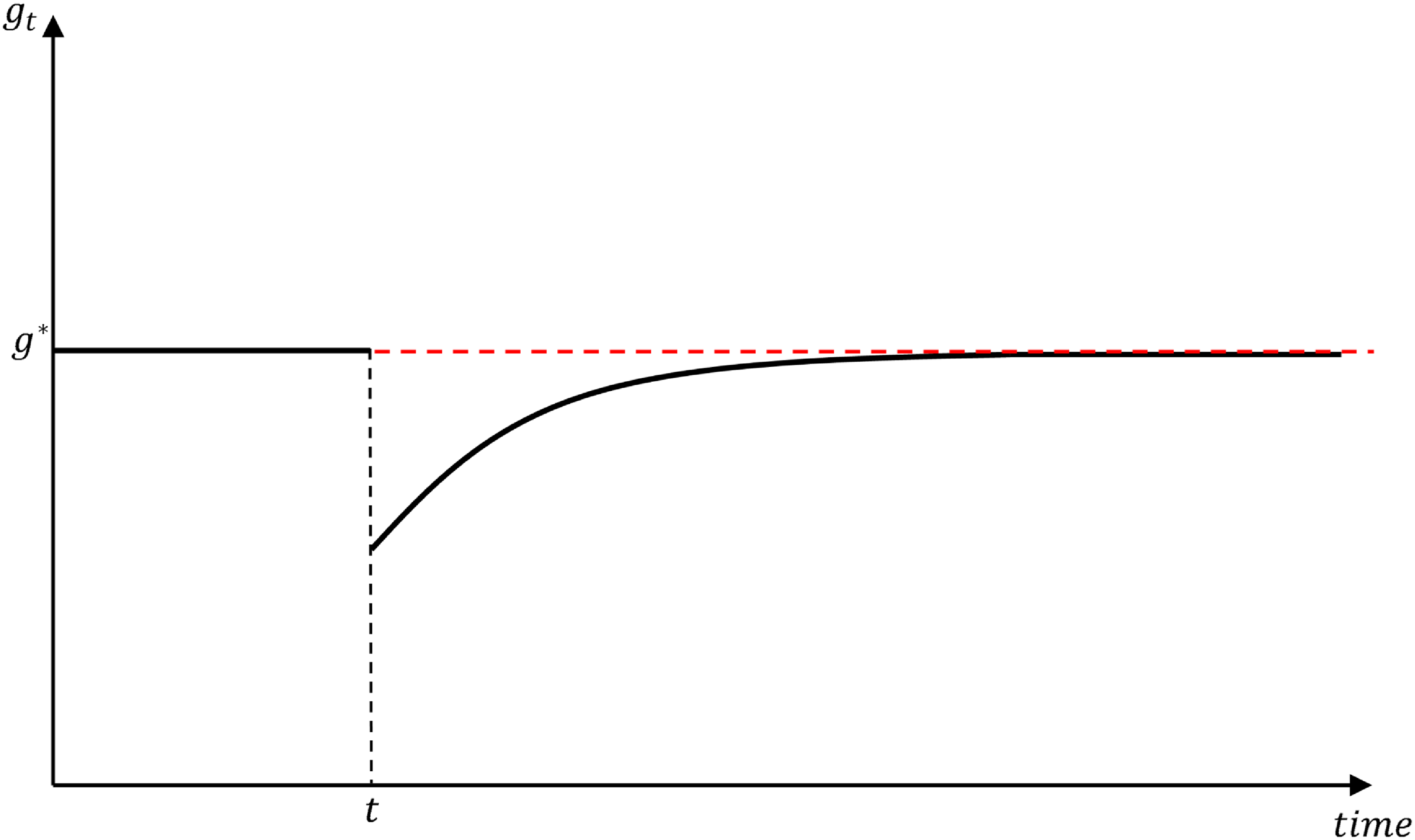
 ω>1
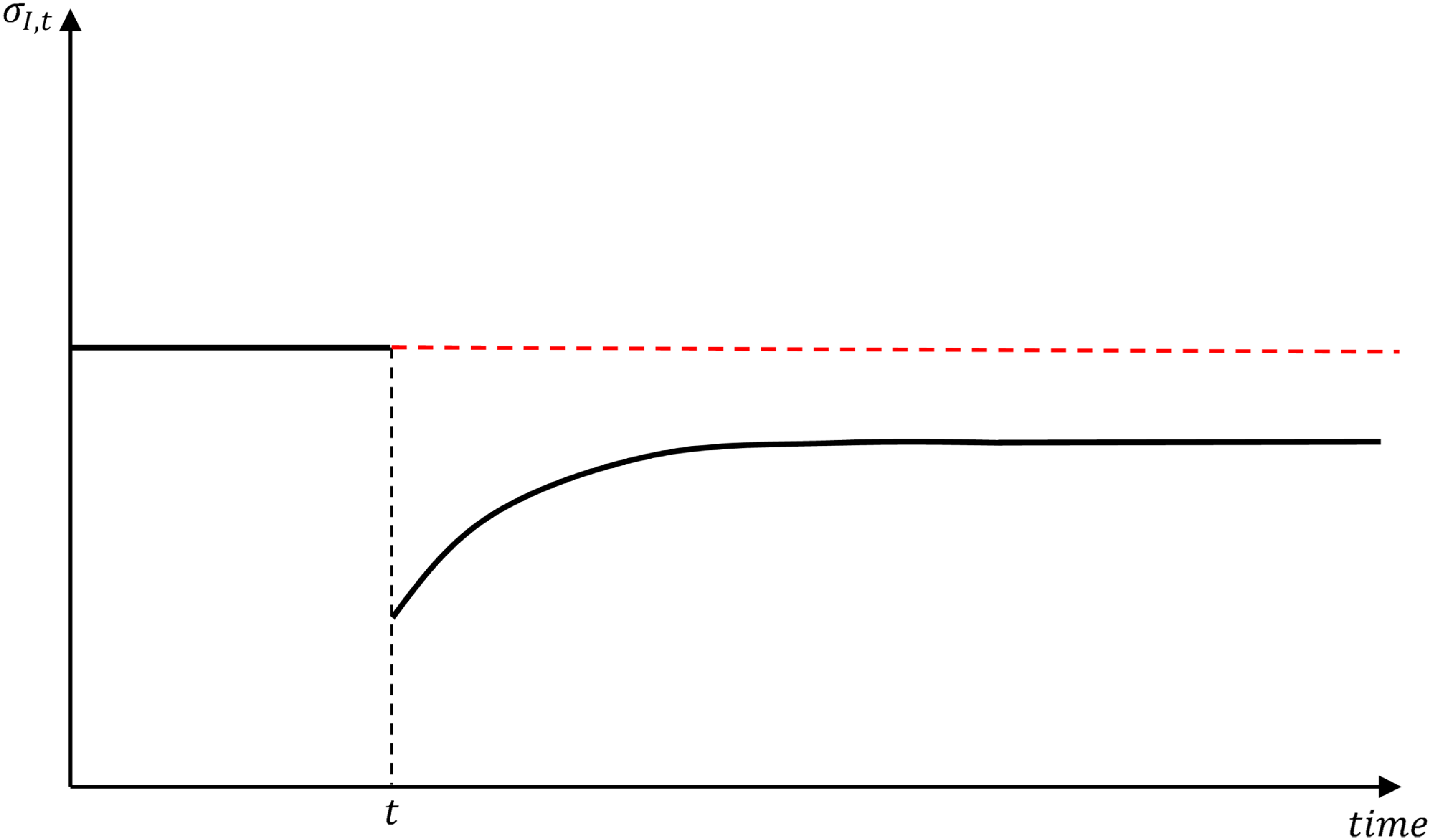
 ω>1
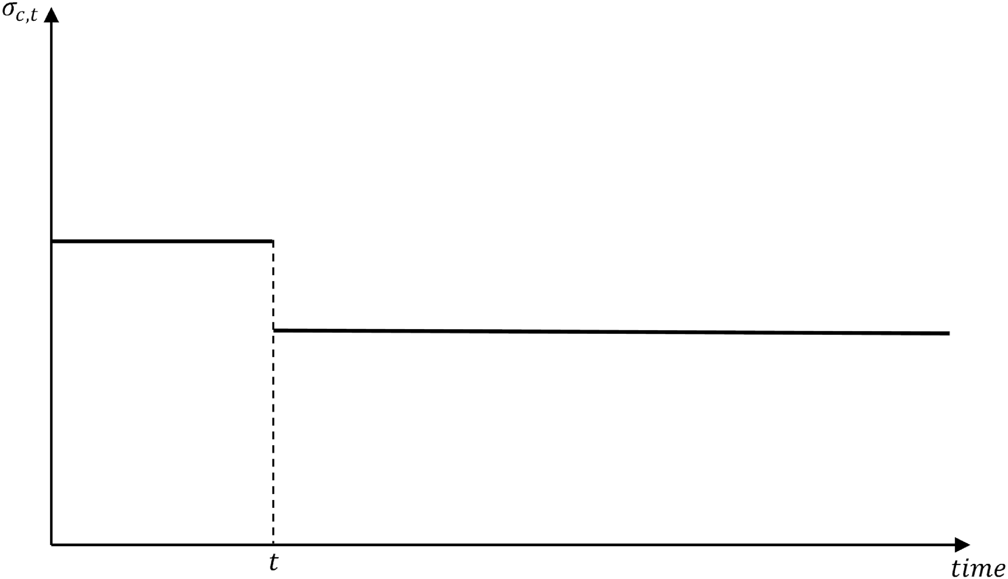


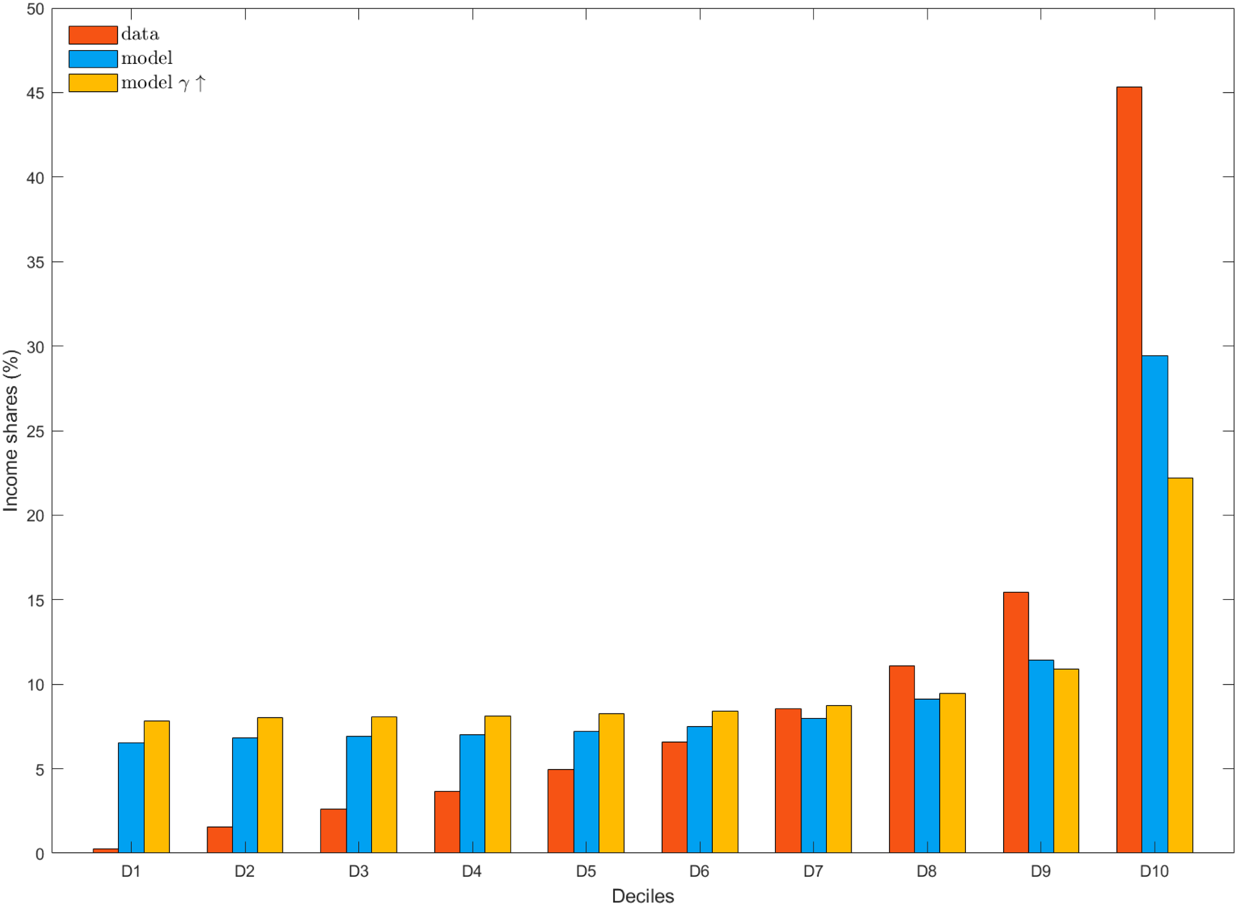

 γ





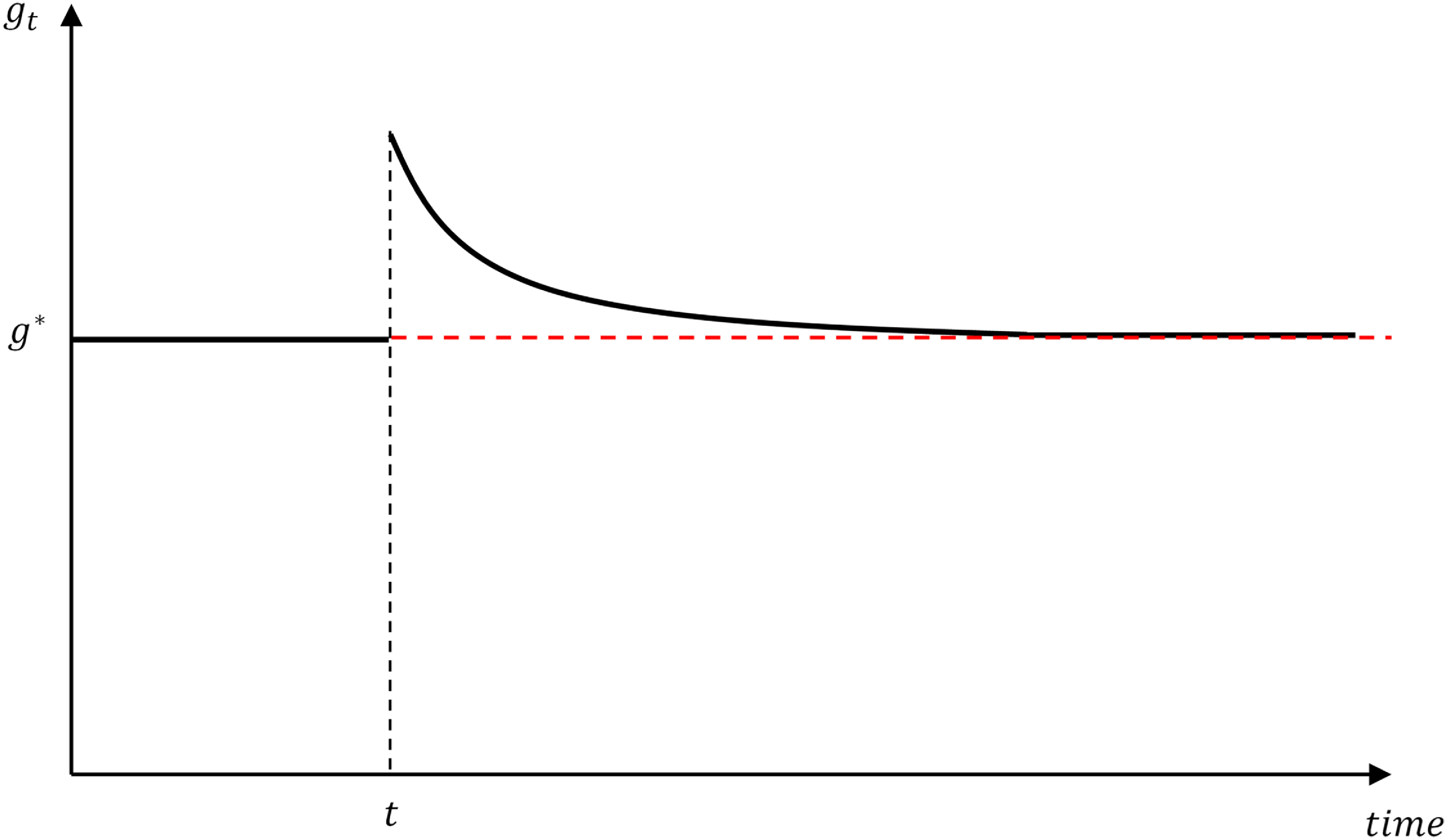
 ω<1
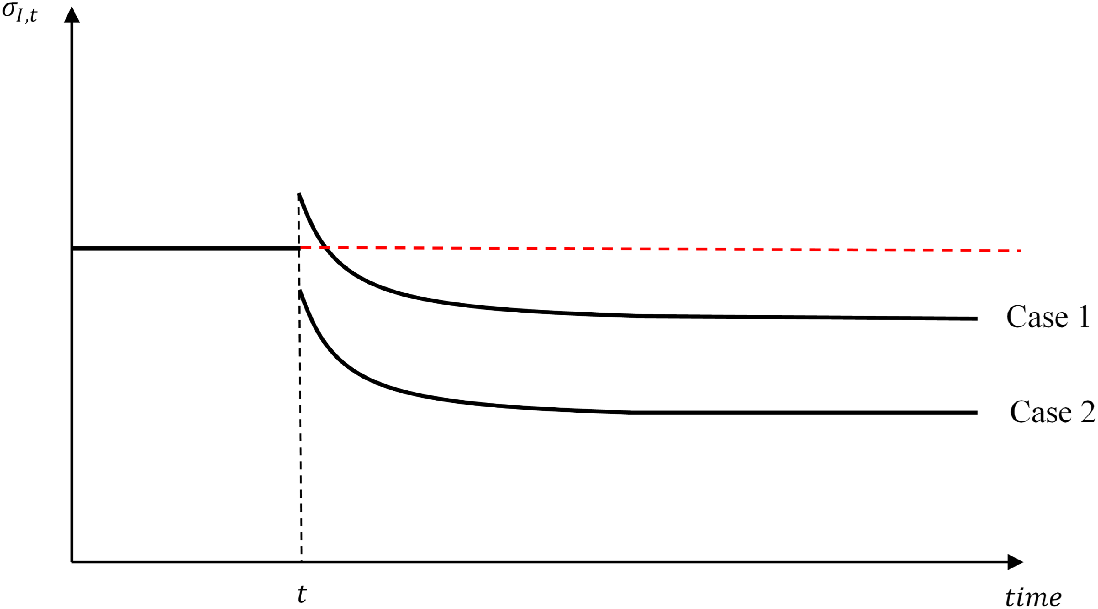
 ω<1


