





1. Introduction
The flow-induced flutter of a three-dimensional (
 $3$
-D) flexible plate is a fundamental phenomenon with significant implications across various physical and engineering domains. For example, it underlies natural processes such as aquatic animal propulsion (Lighthill Reference Lighthill1960; Lighthill Reference Lighthill1970; Wu Reference Wu1971), avian flight (Lighthill Reference Lighthill1975; Tucker Reference Tucker1987) and the biomechanics of human snoring (Aurégan & Depollier Huang Reference Huang1995; Balint & Lucey Reference Balint and Lucey2005; Balint & Lucey Reference Balint and Lucey2005). Moreover, this phenomenon is critical in understanding aeroelastic instabilities in aerospace structures, including aircraft wings (Hodges et al. Reference Hodges, Patil and Chae2002; Berci & Torrigiani Reference Berci and Torrigiani2020) and turbine blades (Panovsky Jr Seeley et al. Reference Seeley, Wakelam, Zhang, Hofer and Ren2017; Seeley et al. Reference Seeley, Wakelam, Zhang, Hofer and Ren2017). In addition, in the emerging field of flow-induced energy harvesting (Tang et al. Reference Tang, Païdoussis and Jiang2009; Akcabay & Young Reference Akcabay and Young2012; Michelin & Doaré Zargarani & Mahmoodi Reference Zargarani and Mahmoodi2015; Latif et al. Reference Latif, Dowell, Uddin, Younis and Frisch2024; Latif et al. Reference Latif, Dowell, Uddin, Younis and Frisch2024), flutter is harnessed to convert kinetic energy of the fluid into usable electrical power.
The study of flow-induced vibrations of flexible plates has captivated researchers for over a century, with early investigations predominantly centred on theoretical analyses of the two-dimensional (
 $2$
-D) case. In his famous paper on the instability of jets, Rayleigh (Reference Rayleigh1878) derived a formula for the fluid loading on an infinite horizontal surface and hypothesised that his theoretical framework could be used to demonstrate the inherent instability of an infinite plate. In their theoretical and experimental study, Kornecki et al. (Reference Kornecki, Dowell and O’brien1976) conducted an in-depth analysis on the aeroelastic instability of a panel with various boundary conditions on its leading edge and trailing edge (TE), fully immersed in an incompressible, 2-D air flow. Their findings demonstrated that a plate with infinite span and finite chord remained stable at flow velocities below a critical threshold. Garrad & Carpenter (Reference Garrad and Carpenter1982) applied thin airfoil theory to compute the aerodynamic forces but introduced a correction factor to account for the effects of the boundary layer. Lucey & Carpenter (Reference Lucey and Carpenter1993) theoretically investigated the linear stability of a compliant panel with a finite aspect ratio fixed to a rigid wall. Their analysis revealed that a compliant wall of finite length is inherently more stable than one with infinite span. Their work can be seen as a 3-D extension of the study conducted by Kornecki et al. (Reference Kornecki, Dowell and O’brien1976).
More recently, Argentina & Mahadevan (Reference Argentina and Mahadevan2005) studied the onset of instability of a plate with a 2-D model based on the work of Theodorsen (Reference Theodorsen1935) and Kornecki et al. (Reference Kornecki, Dowell and O’brien1976). They discussed the stabilising influence of finite
 $3$
-D wavelengths using a
 $2$
-D flag model with data from a
 $3$
-D simulation and showed that the instability threshold is higher in the presence of spanwise modes. Another theoretical approach was presented by Guo & Païdoussis (Reference Guo and Païdoussis2000) for rectangular, infinite-span plates with free side edges in a 2-D inviscid fluid. They derived two equations in the frequency domain for the velocity potential: one governing the pressure and the other being the Laplace equation. These equations can be solved with appropriate boundary conditions and the Galerkin method is then applied to the one-dimensional equation of motion of the plate. Eloy et al. (Reference Eloy, Souilliez and Schouveiler2007) extended this approach to three dimensions by incorporating the finite span of the plate. This new theory assumes that the flutter modes remain 2-D, the fluid is inviscid, and viscoelastic damping is negligible. A key finding of this work is that an infinite-span plate is less stable than a finite-span plate. Alben & Shelley (Reference Alben and Shelley2008) investigated the instability of an inextensible flexible sheet in inviscid
 $2$
-D flow, where the wake is represented with a free vortex sheet. In comparison with experiments, they observed hysteresis. To explain the discrepancies, they proposed a hypothesis suggesting that dissipative effects, such as viscosity or structural damping, could be the underlying cause. Michelin et al. (Reference Michelin, Smith and Glover2008) developed a 2-D vortex-shedding model to describe the flapping of an elastic, inextensible, infinitely thin flag of finite length in axial flow. Their analysis identified direct kinematic waves travelling with the flow and reversed dynamic waves propagating upstream, transmitting pressure variations from vortex shedding. Their stability curves agree well with the results of Kornecki et al. (Reference Kornecki, Dowell and O’brien1976) and Alben & Shelley (Reference Alben and Shelley2008), although their model still underpredicts the width of the hysteresis cycle when compared with experimental data (Eloy et al. Reference Eloy, Lagrange, Souilliez and Schouveiler2008).
The papers discussed above focused solely on inviscid flows; however, recent developments in this field have expanded to include considerations of viscous effects. Building on the work of Triantafyllou (Reference Triantafyllou1992) and Coene (Reference Coene1992); Connell & Yue (Reference Connell and Yue2007) studied theoretically and numerically the dynamics of a 2-D, thin flag in a uniform flow. Their linear stability analysis provides an analytical formula for the critical parameters and incorporates the stabilising effect of varying tension in the flag. In order to investigate the dynamics of flags in the limit of small bending rigidity, Banerjee et al. (Reference Banerjee, Connell and Yue2015) extended this model to three dimensions, while neglecting the stabilising influence of bending rigidity and the effects of finite span with vortex shedding, both of which have been shown to enhance stability (Eloy et al. Reference Eloy, Souilliez and Schouveiler2007).
In recent years, considerable efforts have been made to gain a deeper understanding of the underlying physics of flow-induced, self-sustained flutter through numerical simulations. Huang & Sung (Reference Huang and Sung2010) conducted a series of systematic 3-D simulations to study flexible plates in a uniform stream with low-to-moderate mass ratios and two different aspect ratios, utilising fluid–structure interaction (FSI) based on the immersed boundary method. They explored the effect of Reynolds number on the behaviour of the structure and demonstrated the emergence of asymmetric flapping at higher Reynolds numbers. They also identified the presence of hairpin or O-shaped vortical structures behind the flag and established a relationship between the Strouhal number and the density ratio. Since its publication, this work has also served as a benchmark for validating FSI codes, see Tian et al. (Reference Tian, Dai, Luo, Doyle and Rousseau2014) and Ma et al. (Reference Ma, Wang, Young, Lai, Sui and Tian2020), among others. Specifically, de Tullio & Pascazio (Reference de Tullio and Pascazio2016) proposed a versatile moving-least-squares immersed boundary method (MLS/IBM), where the structural dynamics of the plate is solved using an effective spring-network approach.
Regarding the energy harvesting capability of this system, a number of studies have investigated the energy conversion potential, mostly focusing on inverted plates (Kim et al. Reference Kim, Cossé, Cerdeira and Gharib2013; Gurugubelli & Jaiman Reference Gurugubelli and Jaiman2015; Ryu et al. Reference Ryu, Park, Kim and Sung2015; Tang et al. Reference Tang, Liu and Lu2015). In particular, Ryu et al. (Reference Ryu, Park, Kim and Sung2015) compared the mean bending energy of inverted and standard plates through numerical simulations performed over a range of bending rigidities and Reynolds numbers. For the conditions investigated therein, however, the standard plate either did not exhibit self-sustained flapping or exhibited a substantially lower mean bending energy than the inverted plate. A similar result was also observed by Gurugubelli & Jaiman (Reference Gurugubelli and Jaiman2015), when comparing the mean bending energy of a flexible foil in inverted and standard configurations. A relevant contribution has been given by Michelin & Doaré (Reference Michelin and Doaré2013), who studied piezoelectric flags with an aspect ratio of
 $\mathcal{AR} = 0.5$
and clamped at the leading edge. They showed that the harvesting efficiency strongly depends on the piezoelectric coupling, flow velocity and tuning between the fluid–solid and electrical systems, with power extraction reaching up to
 $10\,\%$
of the incoming kinetic energy flux.
Despite substantial progress in the field, a comprehensive understanding of the flapping dynamics induced by self-excited excitation across the full range of relevant non-dimensional parameters remains elusive. So far, most existing studies have been confined to relatively narrow regions of the parametric space, thereby limiting the generalisability and broader applicability of their conclusions. In contrast, the present study undertakes a systematic exploration of the governing parametric space associated with the flapping dynamics of a rectangular plate in viscous flow. We explore previously unexplored regions of the parametric space, precisely delineating both the onset of flapping from the steady state and the transitions between distinct flapping modes. The numerical results have been rationalised by extending the instability criterion of Banerjee et al. (Reference Banerjee, Connell and Yue2015) to account for the effect of plate rigidity. This extensive analysis yields a deeper insight into the onset, evolution and classification of distinct flapping regimes, while simultaneously establishing the viability of the conventional flapping plate configuration (i.e. hinged at the leading edge) as a mechanism for fluid–structure energy harvesting.
2. Problem description and numerical methods
Let us consider a 3-D plate subjected to a uniform inflow. A schematic representation of the problem is shown in figure 1, where a square plate (
 $L=W$
) with chord length
 $L$
and span
 $W$
is pinned at the leading edge, while the side edges and TE are free. The origin of the reference Cartesian coordinate system is positioned at the centre of the leading edge and the Navier–Stokes equations are solved in a rectangular box of size
 $[-L, L] \times [-3L,3L] \times [-L,3L]$
in the
 $x$
-spanwise,
 $y$
-transverse and
 $z$
-streamwise directions, respectively. The domain extensions employed in this study are justified based on the sensitivity analysis reported in Appendix A. The plate is initially flat, inclined at an angle of
 $0.1\pi$
relative to the x–z plane to introduce a perturbation to the equilibrium configuration, triggering the onset of instability (as prescribed in Huang & Sung Reference Huang and Sung2010). Dirichlet boundary conditions (
 $u = U$
,
 $v = w = 0$
) are applied at the inflow (
 $z = -L$
), along with a convective condition (
 $ {\partial {u}}/{\partial t} + U ({\partial {u}}/{\partial z}) = 0$
) at the outflow (
 $z = 3L$
). Periodic boundary conditions are imposed in the
 $x$
and
 $y$
directions. A no-slip condition is enforced on the surface of the plate.
Three-dimensional representation of a square flapping plate of length
 $L$
hinged at the leading edge and subjected to a uniform incoming flow with velocity
 $U$
.

The fluid density
 $\rho _{f}$
, fluid velocity
 $U$
and length
 $L$
are used to introduce the following four dimensionless parameters:
 \begin{align} Re_L = \frac {UL}{\nu }, \quad M_s=\frac {\rho _{s}h}{\rho _{f}L}, \quad S=\frac {Eh}{\rho _{f}U^{2}L}, \quad K_{B}=\frac {B}{\rho _{f}U^{2}L^{3}}, \end{align}
which represent the Reynolds number, the mass ratio and the non-dimensional stretching and bending stiffnesses, respectively. In (2.1),
 $\nu$
denotes the kinematic viscosity of the fluid,
 $\rho _s$
is the structural density,
 $h$
is the plate thickness and
 $E$
is the Young’s modulus of the material. The bending rigidity of the plate is defined as
 $ B= {Eh^{3}}/{12 ( 1-\nu _s^{2} )}$
, where
 $\nu _s$
is the Poissons’ ratio. The plate is considered inextensible, a condition ensured by prescribing a sufficiently large non-dimensional elastic modulus,
 $S = 1000$
, which is held fixed across all simulations. Consequently,
 $S$
and the non-dimensional bending rigidity,
 $K_B$
, are effectively decoupled, allowing
 $K_B$
to be varied independently.
In the following, we explore a wide range of
 $M_s$
(varying from
 $0.01$
to
 $100$
) and
 $K_B$
(between
 $10^{-4}$
and
 $10^{-1}$
) for a lower
 $( \textit{Re}_L =200)$
and a higher
 $( \textit{Re}_L=1000)$
Reynolds number.
2.1. Fluid–structure interaction
The 3-D viscous flow around the plate is obtained through the direct numerical simulation of the incompressible fluid momentum
 \begin{align} \frac {\partial \boldsymbol{u}}{\partial t}+\boldsymbol{u} \,\boldsymbol{\cdot }\, \boldsymbol{\nabla }\boldsymbol{u}= -\boldsymbol{\nabla }p+\frac {1}{Re}\boldsymbol{\nabla} ^2 \boldsymbol{u}+ \boldsymbol{f}, \end{align}
and continuity equations
 \begin{align} \boldsymbol{\nabla }\boldsymbol{\cdot }{\boldsymbol u}=0, \end{align}
where
 $\boldsymbol{u} = [ u \quad v \quad w ]^{{T}}$
is the fluid velocity vector,
 $p$
represents the pressure and
 $\boldsymbol{f}$
is the MLS/IBM forcing term (Vanella & Balaras Reference Vanella and Balaras2009).
Equations (2.2) and (2.3) are solved numerically using an in-house finite-difference solver, which has been extensively validated and is fully GPU-accelerated for efficient simulation of FSI problems (Viola et al. Reference Viola, Spandan, Meschini, Romero, Fatica, de Tullio and Verzicco2022, Reference Viola, Del Corso and Verzicco2023). Spatial derivatives are discretised on a uniform, homogeneous staggered mesh using central, second-order finite differences. Time integration is carried out using an implicit Crank–Nicolson scheme for the linear viscous terms and an explicit Adams–Bashforth scheme for the nonlinear terms. Pressure and momentum are loosely coupled through a fractional-step method (Verzicco & Orlandi Reference Verzicco and Orlandi1996). For the computation of pressure and viscous stresses, the physics-based correction proposed by Wang et al. (Reference Wang, Vanella and Balaras2019) is adopted. For a detailed description of the numerical methods employed in the solver, the reader is referred to Verzicco et al. (Reference Verzicco, de Tullio and Viola2025).
To model the dynamics of the deformable plate, a spring-network model (Gelder Reference Gelder1998) based on the interaction potential method (Fedosov et al. Reference Fedosov, Caswell and Karniadakis2010) is adopted, in which the continuum is discretised by
 $N_{t}$
triangles and the mass of the structure is distributed among the
 $N_{v}$
element nodes. In-plane stiffness is introduced by placing a spring at each edge of the triangular network, while the bending stiffness of the shell is obtained through out-of-plane springs that link the centroids of two neighbouring triangular faces sharing a common edge. In this section, we provide a brief introduction of the key concepts; for a detailed overview, the reader is referred to de Tullio & Pascazio (Reference de Tullio and Pascazio2016) and Viola et al. (Reference Viola, Meschini and Verzicco2020).
The elastic constant for a given edge of length
 $l$
is obtained as
 \begin{align} k_{e}=\frac {Eh\sum _{i}A_{i}}{l^{2}}, \end{align}
where the index
 $i$
identifies the triangles sharing the selected edge (here two triangles) and
 $A_i$
is the triangle area. The out-of-plane deformation between two adjacent triangles sharing a common edge is represented by a bending spring, with the associated bending energy depending on the four nodes that define these triangles. For the case of a surface with non-zero reference curvature, the bending energy is calculated as
 \begin{align} {E}_B=k_{b}\left [ 1-\text{cos}\left ( \varTheta -\varTheta _{0} \right ) \right ], \end{align}
where
 $\varTheta$
denotes the actual dihedral angle between the normals of two adjacent triangular faces and
 $\varTheta _{0}$
represents its value in the undeformed (stress-free) configuration. The bending constant
 $k_b$
is related to the bending rigidity
 $B$
of the elastic structure through the expression
 $k_b = 2B/\sqrt {3}$
. Once these two structural quantities are specified, the dynamic equation of motion can be solved for each node of the triangulated mesh, taking into account both external hydrodynamic forces and internal elastic forces.
2.2. Linear stability analysis
In this section, we review the linear stability model of Banerjee et al. (Reference Banerjee, Connell and Yue2015), which generalises the 2-D framework of Connell & Yue (Reference Connell and Yue2007) to three dimensions, and extend the formulation by incorporating the effects of bending rigidity. The equation of motion for a thin, flexible plate can be expressed as follows:
 \begin{align} \begin{split} \rho _{s}h\frac {\partial ^2 \eta }{\partial t^2}-\frac {\partial }{\partial x}\left ( T_{x}\frac {\partial \eta }{\partial x}\right )-\frac {\partial }{\partial z}\left ( T_{z}\frac {\partial \eta }{\partial z}\right )+B\frac {\partial ^{4}\eta }{\partial x^{4}}+2B\frac {\partial ^{4}\eta }{\partial x^{2}\partial z^{2}}+B\frac {\partial ^{4}\eta }{\partial z^{4}}+\Delta P\left ( z;t \right )=0, \end{split} \end{align}
where
 $\eta (x,z;t)$
denotes the displacement of the structure from the
 $y=0$
plane. The first term describes the inertial response of the plate, while the second and third terms account for the tension in the spanwise and streamwise directions, respectively. The next three terms capture the effect of bending rigidity. The final term,
 $\Delta P(z;t)$
, represents the pressure difference acting across the surface of the plate, accounting for the effect of the added mass of the fluid,
 $m_a$
. The fluid forcing is expressed using the formula derived by Rayleigh (Reference Rayleigh1878) and Lamb (Reference Lamb1924):
 \begin{align} \Delta P\left ( z;t \right )=m_{a}\left ( \frac {\partial }{\partial t}+U\frac {\partial }{\partial z} \right )^{2}\eta . \end{align}
Following previous studies (Connell & Yue Reference Connell and Yue2007; Banerjee et al. Reference Banerjee, Connell and Yue2015), the streamwise tension is considered constant over the plate and is set equal to the Blasius boundary-layer solution evaluated at the leading edge,
 $T_{z}=C_{T} \rho _{f}U^{2}LRe_{L}^{-1/2}$
, while the spanwise tension is scaled by the Poisson’s ratio as
 $T_{x}=\nu _{s}T_{z}$
. The variables
 $ (x, z, \eta , t )$
in (2.6) are now made non-dimensional using the characteristic velocity
 $U$
and length scale
 $L$
, yielding
 \begin{align} \begin{split} \left ( M_{s}+c_{m} \right )\frac {\partial ^{2}\eta }{\partial t^{2}}-C_{T}\nu _{s}Re_{L}^{-1/2}\frac {\partial ^{2}\eta }{\partial x^{2}}+\big ( c_{m}- C_{T} Re_{L}^{-1/2}\big )\frac {\partial ^{2}\eta }{\partial z^{2}}+\\[4pt]2c_{m}\frac {\partial ^{2}\eta }{\partial t \partial z}+K_{B}\frac {\partial ^{4}\eta }{\partial x^{4}}+2K_{B}\frac {\partial ^{4}\eta }{\partial x^{2}\partial z^{2}}+K_{B}\frac {\partial ^{4}\eta }{\partial z^{4}} = 0, \end{split} \end{align}
where
 $C_{T}=1.328$
is the tension coefficient and
 $c_{m}=m_{a}/\rho _{f}L$
is the added mass coefficient. In this study, we adopt the expression
 $m_{a}= ({\rho _{f}L}/{\pi }) ({W}/{L}) ( {\pi }/{2} )^{2}$
derived by Wu (Reference Wu1971). Following Banerjee et al. (Reference Banerjee, Connell and Yue2015), we consider a mode shape corresponding to a standing wave in the spanwise
 $x$
direction and a travelling wave in the streamwise
 $z$
direction, given by
 $\eta = ({A}/{2}){\rm e}^{{\rm i} ( k_{z}z-\omega _{\textrm{3-D}} t )}\cos ( k_{x}x )$
, where
 $A$
is the peak-to-peak flapping amplitude,
 $\omega _{\textrm{3-D}}$
is the complex frequency and
 $k_x$
and
 $k_z$
are the spanwise and streamwise wavenumbers, respectively. Substituting this modal shape into (2.8) yields the dispersion relation
 \begin{align} \begin{split} \left ( M_{s} + c_{m} \right ) \omega _{\textrm{3-D}}^{2}- C_{T}\nu _{s} Re_{L}^{-1/2} k_{x}^{2}+ \big ( c_{m}- C_{T} Re_{L}^{-1/2}\big )k_{z}^{2} - \\[4pt]2 c_{m} k_{z} \omega _{\textrm{3-D}}- K_{B} k_{x}^{4}- 2K_{B}k_{x}^{2}k_{z}^{2} - K_{B} k_{z}^{4} = 0. \end{split} \end{align}
The complex frequency can then be expressed as
 \begin{align} \omega _{\textrm{3-D}}^{\pm }=\frac {c_{m}k_{z}}{M_{s}+c_{m}} \big [ 1\pm \mathscr{P}_{\textrm{3-D}}\left ( k_{x}, k_{z};M_{s}, {K_B} \right )^{1/2} \big ], \end{align}
where
 \begin{align} \begin{aligned} \mathscr{P}_{\textrm{3-D}}\left ( k_{x}, k_{z};M_{s}, {K_B} \right ) &= \Big [ - M_{s}c_{m}k_{z}^{2} + \left ( M_{s}+c_{m} \right ) \left ( \mathscr{A}\left ( k_{x}; {K_B} \right )+ \right . \\&\left . \mathscr{B}\left ( k_{z};{K_B} \right ) + \mathscr{C}\left ( k_{x},k_{z};{K_B} \right ) \right ) \Big ] \Big / \left ( c_{m}k_{z} \right )^{2}, \end{aligned} \end{align}
with
 $\mathscr{A} ( k_{x};{K_B} )=C_{T}\nu _{s} Re_{L}^{-1/2}k_{x}^{2}+K_{B}k_{x}^{4}$
,
 $\mathscr{B} ( k_{z};{K_B} )=C_{T} Re_{L}^{-1/2}k_{z}^{2}+K_{B}k_{z}^{4}$
and
 $\mathscr{C} ( k_{x},k_{z};{K_B} )=2K_{B}k_{x}^{2}k_{z}^{2}$
. Unstable flapping modes occur when
 $\mathscr{P}_{\textrm{3-D}} ( k_{x}, k_{z};M_{s},{}{K_B} ) \lt 0$
. From this criterion, instability conditions on bending rigidity and critical mass ratio can be expressed as
 \begin{align} K_{B}\lt K_B^{\textit{crit}}=\frac {M_{s}c_{m}k_{z}^{2}-C_{T}Re_{L}^{-1/2}\left ( M_{s}+c_{m} \right )\left ( \nu _{s}k_{x}^{2}+k_{z}^{2} \right )}{\left ( M_{s}+c_{m} \right )\left ( k_{x}^{4}+k_{x}^{2}k_{z}^{2}+k_{z}^{4} \right )} \end{align}
and
 \begin{align} M_{s}\gt M_s^{\textit{crit}}=\frac {c_{m}\left [ C_{T}Re_L^{-1/2}\left ( \nu _{s}k_{x}^{2}+k_{z}^{2} \right )+K_{B}\left ( k_{x}^{4}+2k_{x}^{2}k_{z}^{2}+k_{z}^{4} \right ) \right ]}{c_{m}k_{z}^{2}-C_{T}Re_L^{-1/2}\left ( \nu _{s}k_{x}^{2}+k_{z}^{2} \right )-K_{B}\left ( k_{x}^{4}+2k_{x}^{2}k_{z}^{2}+k_{z}^{4} \right )}. \end{align}
For predicting the onset of flapping instability, it is reasonable to assume that
 $\eta (x,z;t)=\eta (z;t)$
(see § 3.2). Under this assumption,
 $k_{x}=\mathscr{A}=\mathscr{C}=0$
, and (2.12) and (2.13) reduce to the form obtained by Connell & Yue (Reference Connell and Yue2007) for an infinite-span (effectively 2-D) plate. The only difference lies in the added-mass coefficient: Connell & Yue (Reference Connell and Yue2007) considered
 $c_m = 2/k_z$
for an infinite waving structure, whereas (2.12) and (2.13) employ
 $c_m = W\pi /(4L)$
, appropriate for a finite-aspect-ratio plate. As a final remark, since the present analysis retains the bending rigidity of the plate, the marginal stability curves depend on both
 $K_B$
and the longitudinal wavenumber, unlike the wavenumber-independent limit obtained when
 $K_B$
is neglected, as in Banerjee et al. (Reference Banerjee, Connell and Yue2015).
Comparing the streamwise tension
 $T_z$
at
 $ \textit{Re}_L = 200$
and
 $ \textit{Re}_L = 1000$
, we find that the restoring effect is more than twice as strong at
 $ \textit{Re}_L = 200$
, due to its inverse dependence on the Reynolds number. Focusing on the streamwise bending contribution (sixth term in (2.6)) and considering the lowest wavenumber,
 $k_z = 2\pi$
, we obtain that the inequality
 $K_B k_z^4 \gt C_TRe_L^{-1/2} k_z^2$
is satisfied for
 $K_B \approx 2.4 \times 10^{-3}$
at
 $ \textit{Re}_L = 200$
. At
 $ \textit{Re}_L = 1000$
, the same inequality holds for an even smaller value,
 $K_B \approx 1.1 \times 10^{-3}$
, indicating that bending effects dominate over the tension term in most of the parameter regime considered in this study. This dominance becomes even more pronounced as either
 $K_B$
or
 $ \textit{Re}_L$
increases. For higher-order modes (i.e. larger wavenumbers), the critical value of
 $K_B$
required to satisfy
 $K_B k_z^4 \gt C_TRe_L^{-1/2} k_z^2$
becomes even smaller, further emphasising the increasing importance of bending at smaller spatial scales.
3. Results
3.1. Representative cases of plate dynamics
In this section, we provide an overview of the flapping regimes of a flexible plate by reporting the transverse motion of the three TE points indicated in figure 1 for three different mass ratios (
 $M_s={\{}0.1, 10, 100{\}}$
) at
 $ \textit{Re}_L = 200$
and
 $ \textit{Re}_L = 1000$
, with a bending rigidity of
 $K_B =10^{-4}$
.
Time histories of the transverse displacements of the mid- and sidepoints of the TE of the plate, shown relative to their equilibrium positions. Results are presented for
 $ \textit{Re}_L=200$
and
 $ \textit{Re}_L=1000$
with
 $(a{,}b)$
 $M_s = 0.1$
,
 $(c{,}d)$
 $M_s = 1$
and
 $(e{,}f)$
 $M_s = 10$
, and a bending rigidity of
 $K_B =10^{-4}$
.

In figure 2
 $(a)$
, at
 $M_s = 0.1$
and
 $ \textit{Re}_L = 200$
, after a brief transient, the plate rapidly relaxes to its equilibrium position (
 $y = 0$
) and remains in a flat, stable configuration. However, at the same mass ratio, the plate exhibits markedly different behaviour at
 $ \textit{Re}_L = 1000$
, as shown in figure 2
 $(b)$
: it undergoes a limit-cycle flapping motion, characterised by small peak-to-peak amplitudes
 $A/L$
and a high Strouhal number
 $ \textit{St}_L= {fL}/{U}$
, where
 $f$
is the flapping frequency measured for the midpoint of the TE. The differing stability characteristics observed at
 $ \textit{Re}_L = 200$
and
 $ \textit{Re}_L = 1000$
arise from the Reynolds-number dependence of the viscous forces, which exert a progressively weaker stabilising influence as
 $ \textit{Re}_L$
increases. As is evident from (2.9), the viscous damping scales as
 $ \textit{Re}_L^{-1/2}$
, and thus the stabilising effect diminishes with increasing
 $ \textit{Re}_L$
. Consequently, a higher
 $ \textit{Re}_L$
number expands the unstable domain.
Figure 2
 $(c)$
illustrates that, for a moderate mass ratio
 $M_s = 1$
and a low Reynolds number
 $ \textit{Re}_L = 200$
, the plate exhibits self-sustained limit-cycle oscillations, with negligible differences in peak-to-peak amplitude between the midpoint and the two sidepoints of the TE. This indicates that the motion remains predominantly symmetric and 2-D. As depicted in figure 2
 $(d)$
, at
 $ \textit{Re}_L = 1000$
the transverse displacements at the midpoint and sidepoints initially differ noticeably. Although this discrepancy diminishes after several cycles, it does not vanish entirely and continues to fluctuate over time, suggesting a transition towards 3-D behaviour. In addition, the peak-to-peak amplitude at one of the sidepoints exceeds that at the other one and at the midpoint, indicating the occurrence of a slight asymmetry.
Further increasing the mass ratio to
 $M_s = 10$
produces a high-amplitude, irregular flapping motion, characterised by pronounced variations in the transverse displacement among the three TE points, together with cycle-to-cycle fluctuations in the Strouhal number (see figures 2
e and 2
f). This behaviour is accompanied by the activation of spanwise deformation modes, indicating the occurrence of 3-D dynamics. Such 3-D, irregular flapping is consistently observed at both
 $ \textit{Re}_L$
, further highlighting the dominant influence of inertial effects associated with a large
 $M_s$
.
These observations are further supported by the trajectories of the three TE points, visualised from both the front and side views in figures 3 and 4, respectively. In particular, the characteristic shape of limit-cycle oscillations is progressively lost as
 $M_s$
increases. Moreover, at higher
 $ \textit{Re}_L$
, the flapping becomes increasingly 3-D, as reflected by the growing disparity in the trajectories of the side and midpoint locations.
Front-view trajectories of TE middle (black) and side (red and blue) points at
 $(a$
–
 $c)$
 $ \textit{Re}_L=200$
and
 $(d$
–
 $f)$
 $ \textit{Re}_L=1000$
.

Figure 3. Long description
Panel A: A scatter plot showing the trajectories of the trailing edge (TE) middle (black) and side (red and blue) points at M_s = 0.1 and Re_L = 200. The x-axis is labeled X_TE/L and the y-axis is labeled Y_TE/L, both ranging from -1 to 1. The points are aligned vertically. Panel B: A scatter plot showing the trajectories of the TE middle (black) and side (red and blue) points at M_s = 1 and Re_L = 200. The points are aligned vertically. Panel C: A scatter plot showing the trajectories of the TE middle (black) and side (red and blue) points at M_s = 10 and Re_L = 200. The points form a wider distribution. Panel D: A scatter plot showing the trajectories of the TE middle (black) and side (red and blue) points at M_s = 0.1 and Re_L = 1000. The points are aligned vertically. Panel E: A scatter plot showing the trajectories of the TE middle (black) and side (red and blue) points at M_s = 1 and Re_L = 1000. The points form a wider distribution. Panel F: A scatter plot showing the trajectories of the TE middle (black) and side (red and blue) points at M_s = 10 and Re_L = 1000. The points form a wider distribution.
Side-view trajectories of TE middle (black) and side (red and blue) points at
 $(a$
–
 $c)$
 $ \textit{Re}_L=200$
and
 $(d$
–
 $f)$
 $ \textit{Re}_L=1000$
.

Phase portraits of lift coefficient as a function of the transverse displacement of the TE midpoint, for the same cases considered in figure 4.

To better characterise the relationship between the structural motion and aerodynamic force, in figure 5 we report the phase portraits of the lift coefficient as a function of the transverse displacement of the TE midpoint. The data are plotted after removing the initial transient. For the stable case corresponding to
 $ \textit{Re}_L = 200$
and
 $M_s = 0.1$
, the phase trajectory reduces to a single point at the origin. In contrast, at the same mass ratio but with
 $ \textit{Re}_L = 1000$
, the phase portrait forms a closed, elliptical loop (corresponding to small-amplitude flapping). For all cases in which the plate exhibits flutter, when the TE midpoint reaches its maximum transverse displacement, the plate experiences a negative peak of the lift. Interestingly,
 $M_s = 1$
yields the steepest curve and the highest lift at both
 $ \textit{Re}_L$
, steeper than at
 $M_s = 10$
. This is attributed to the strong spanwise coherence of the structural motion at
 $M_s = 1$
, where the plate dynamics is essentially 2-D and deforms synchronously along the span. In contrast, at
 $M_s = 10$
, different regions of the plate reach their lift maxima at different times. The resulting lift signal is therefore a superposition of phase-shifted contributions, which reduces the overall lift magnitude and leads to less steep and regular phase trajectories.
Vortical structures shed from the flapping plate, shown at an instant when the midpoint of the TE attains its maximum transverse displacement. Results are shown for
 $ \textit{Re}_L = 200$
and
 $ \textit{Re}_L = 1000$
, corresponding to
 $(a, b)$
 $M_s = 0.1$
,
 $(c, d)$
 $M_s = 1$
and
 $(e, f)$
 $M_s = 10$
, at a (non-dimensional) bending rigidity
 $K_B = 10^{-4}$
. Vortical structures are identified using the
 $Q$
-criterion (Hunt et al. Reference Hunt, Wray and Moin1988), with 3-D isosurfaces at
 $Q = 0.1 (U/L)^2$
, coloured according to the (non-dimensional) vorticity magnitude.

Figure 6 shows the corresponding vortical structures shed from the flapping plate when the midpoint of the TE reaches its maximum transverse displacement. For the lower Reynolds number
 $ \textit{Re}_L=200$
at
 $M_s = 0.1$
(see figure 6
a) the system is stable, with the plate essentially undeformed and the flow characterised by a steady laminar boundary layer developing along the plate. At
 $M_s = 1$
(panel c), a symmetric, hairpin-like vortex can be observed, which is consistent with the essentially 2-D flapping motion. At
 $M_s = 10$
(panel e), however, the plate motion appears 3-D, with vortical structures originating from the side edges not connected across the span, but instead forming two elongated, weakly interacting vortex tubes. Moving to
 $ \textit{Re}_L = 1000$
, the case with
 $M_s = 0.1$
(see figure 6
b) becomes unstable, with the flow field showing a regular pattern characterised by three O-shaped vortical structures that are symmetric and approximately aligned in the streamwise direction. At
 $M_s = 1$
(panel d), the vortical structures become less regular, with hairpin-dominated patterns, enhanced vorticity and strong vertical excursions. At
 $M_s = 10$
(panel f), the flow structures become even more disorganised, and hairpin-like structures are no longer present. The vortical structures are more aligned with the streamwise direction, with reduced vertical excursions but strong vorticity, indicative of chaotic flutter.
3.2. Deformation states
Using direct numerical simulations, we systematically investigate the flapping dynamics of the plate for
 $M_s \in [0.01, 100]$
and
 $K_B \in [10^{-4}, 10^{-1}]$
at
 $ \textit{Re}_L=200$
and
 $ \textit{Re}_L=1000$
. Across the post-critical regime, we identify seven characteristic deformation states of the plate, shown in figure 7, namely:
 $(a)$
mode
 $2$
(single-neck mode),
 $(b)$
mode
 $2+3$
(a mixed mode with a single neck),
 $(c)$
mode
 $3$
(double-neck mode),
 $(d)$
mode
 $3+4$
(a mixed mode between the double-neck and triple-neck modes),
 $(e)$
mode
 $4$
(triple-neck mode),
 $(f)$
mode
 $4+5$
(a mixed mode between the triple-neck and quadruple-neck modes) and
 $(g)$
mode
 $5$
(quadruple-neck mode). Mixed modes arise from modal coalescence, where features of two adjacent pure modes coexist. For a comprehensive overview of flow-induced flag vibrations and their associated flapping modes, we refer the reader to the review by Yu et al. (Reference Yu, Liu and Amandolese2019).
Deformation states in terms of superimposed views of the plate:
 $(a)$
mode
 $2$
,
 $(b)$
mode
 $2+3$
,
 $(c)$
mode
 $3$
,
 $(d)$
mode
 $3+4$
,
 $(e)$
mode
 $4$
,
 $(f)$
mode
 $4+5$
and
 $(g)$
mode
 $5$
.

Observed flapping modes in the
 $M_s-K_B$
parametric space at
 $(a)$
 $ \textit{Re}_L=200$
and
 $(b)$
 $ \textit{Re}_L=1000$
.The symbols
 $\bullet$
,
 ,
 ,
 ,
 ,
 ,
 and
 represent fixed-point stability, mode
 $2$
, mode
 $2+3$
, mode
 $3$
, mode
 $3+4$
, mode
 $4$
, mode
 $4+5$
and mode
 $5$
, respectively. In addition, the marginal stability curves according to linear stability analysis are reported for different longitudinal wavenumbers:
 $k_z$
equal to
 $2\pi$
(red),
 $3\pi$
(cyan),
 $4\pi$
(green) and
 $5\pi$
(magenta). The red dotted line corresponds to the critical curve for
 $k_z=2\pi$
according to the stability analysis of Connell & Yue (Reference Connell and Yue2007).

Figure 8 presents a map of the flapping modes in the
 $M_s$
–
 $K_B$
plane. Marker colours distinguish between the various flapping modes. Filled markers denote limit-cycle, self-excited flapping, referred to here as regular, while empty markers indicate weakly irregular or fully chaotic flapping, collectively classified as irregular. Flapping is classified as regular when the cycle-to-cycle variation of both characteristic quantities, the peak-to-peak amplitude
 $A/L$
and the Strouhal number
 $ \textit{St}_L$
, is less than
 $1$
%. Cases with
 $A/L \leqslant 0.1$
are regarded as stable, based on the criterion that the transverse displacement of the TE midpoint remains below 5 % of the plate length.
Fixed-point stability occurs at sufficiently large
 $K_B$
and/or low
 $M_s$
. At
 $ \textit{Re}_L = 200$
when
 $M_{s} \lt 0.15$
, even for
 $K_B = 10^{-4}$
, which is the lowest
 $K_B$
considered, the straight plate configuration is stable. When the Reynolds number is increased to
 $ \textit{Re}_L = 1000$
, the instability region is slightly extended, with the unstable region starting at
 $M_s = 0.05$
with
 $K_B = 10^{-4}$
. Notably, the highest-order flapping response observed, mode
 $5$
(quadruple mode), appears at
 $ \textit{Re}_L=1000$
within the narrow mass ratio range
 $0.05 \leqslant M_s \leqslant 0.1$
and only when
 $K_B = 10^{-4}$
. In addition, the mixed mode
 $4+5$
appears exclusively at
 $ \textit{Re}_L = 1000$
within the interval
 $0.08 \leqslant M_s \leqslant 0.2$
, and only at low
 $K_B$
values. The upper limit for this mode is observed at
 $K_B = 4 \times 10^{-4}$
when
 $M_s = 0.09$
. These findings highlight that the occurrence of high-order flapping modes is restricted to a narrow region in the
 $M_s$
–
 $K_B$
parametric space.
The plate exhibits flutter in mode
 $4$
at
 $ \textit{Re}_L = 200$
when
 $0.15\leqslant M_{s}\leqslant 0.2$
and
 $K_B = 10^{-4}$
, and at
 $ \textit{Re}_L = 1000$
when
 $0.1 \leqslant M_s \leqslant 0.2$
and
 $K_B = 4 \times 10^{-4}$
. The mixed mode
 $3+4$
appears within the range
 $0.2 \leqslant M_s \leqslant 1$
for both Reynolds numbers, occurring at
 $K_B$
values far from the instability threshold. This mode persists up to
 $K_B = 10^{-3}$
and
 $K_B = 2 \times 10^{-3}$
for
 $ \textit{Re}_L = 200$
and
 $ \textit{Re}_L=1000$
, respectively. The double-neck mode (mode
 $3$
) arises for plates with moderate mass ratios when
 $K_B = {10^{-3}}$
, specifically at
 $M_s = 0.7$
for
 $ \textit{Re}_L = 200$
and
 $M_s = 1$
for
 $ \textit{Re}_L = 1000$
. At sufficiently high
 $K_B$
when
 $M_s \geqslant 0.7$
, the plate flutters in mode
 $2+3$
, corresponding to the mixed single-neck flapping mode. The minimum
 $K_B$
required for the onset of this mode is moderately influenced by both
 $M_s$
and
 $ \textit{Re}_L$
. At
 $ \textit{Re}_L = 200$
, the thresholds are
 $K_B = 2 \times 10^{-3}$
at
 $M_s = 0.7$
and
 $K_B = 1 \times 10^{-3}$
at
 $M_s = 1$
. Increasing the Reynolds number to
 $ \textit{Re}_L = 1000$
raises these thresholds to
 $K_B = 4 \times 10^{-3}$
and
 $K_B = 2 \times 10^{-3}$
, respectively. For
 $M_{s} \gt 1$
, the flutter mode becomes independent of
 $K_B$
, with the plate maintaining mode
 $2+3$
in the post-critical regime. A similar trend is observed at
 $ \textit{Re}_L = 1000$
; however, mode 2 is observed close to the marginal stability condition, before switching to mode
 $2+3$
as
 $K_B$
slightly decreases.
The instability onset of the plate can be rationalised through linear stability analysis. Figure 8 also shows the instability thresholds for the transition from the fixed point to the flapping state, obtained using the present linear stability model, with the plate kinematics restricted by setting
 $k_x=0$
in (2.12), and the model proposed by Connell & Yue (Reference Connell and Yue2007). Under this restriction, the two models are identical except for the added mass coefficient used in the two formulations, as discussed in § 2.2. It results that the stability curve corresponding to mode 2 (
 $k_z=2\pi$
) provides a good prediction of the onset of the flapping instability, particularly at low-to-moderate mass ratios (i.e.
 $M_s \lesssim 1$
). However, the dominant mode observed in the direct numerical simulations in the vicinity of the transition from the stable to the unstable regime is generally different from mode
 $2$
. Depending on
 $M_s$
and
 $K_B$
, different modal responses may arise, including the mixed mode
 $3+4$
observed at
 $ \textit{Re}_L = 200$
for
 $M_s = 0.2$
with
 $K_B = 4 \times 10^{-4}$
, and at
 $ \textit{Re}_L = 1000$
for
 $0.2 \leqslant M_s \leqslant 0.4$
with
 $K_B = 2 \times 10^{-3}$
. At lower mass ratios, even higher-order modes are detected at the onset of instability, such as mode
 $4$
at
 $ \textit{Re}_L = 200$
for
 $M_s = 0.15$
and mode
 $5$
for
 $0.05 \leqslant M_s \leqslant 0.1$
at
 $ \textit{Re}_L = 1000$
, both at
 $K_B = 10^{-4}$
. This behaviour suggests the presence of a nonlinear mechanism in which the initially unstable mode
 $2$
may trigger higher-order modes. While such a mechanism cannot be captured within a linear stability framework, it is consistent with the fact that the marginal stability curves of higher modes approach that of mode
 $2$
at
 $M_s \approx 0.1$
. As a result, when the mass ratio exceeds the critical threshold predicted by mode
 $2$
, higher-order modes, although still linearly stable, are only weakly damped and may get excited nonlinearly and resonate.
Furthermore, at high
 $M_s$
, the predictive capability of the linear stability analysis becomes less accurate, especially for
 $ \textit{Re}_L = 1000$
. This discrepancy likely stems from the local nature of the analysis: the normal-mode ansatz adopted in § 2.2 assumes an infinitely long plate and therefore does not satisfy the pinned–free boundary conditions of the finite plate. Such an approximation is valid when the plate length
 $L$
is much larger than the modal wavelength
 $2\pi /k_z$
, but it breaks down at low wavenumbers, where the wavelength becomes comparable to the flag length. Consistently, the largest discrepancy occurs for
 $M_s \geqslant 2$
, where direct numerical simulation predicts only mode
 $2$
and mode
 $2+3$
, characterised by a relatively large wavelength. Nevertheless, in all cases considered, our stability analysis provides improved predictions compared with those of Connell & Yue (Reference Connell and Yue2007) (indicated by the red dotted line for
 $k_z=2\pi$
).
It is observed that for small values of
 $M_s$
, the stable region is broader, whereas the range for flapping states is narrower than for large
 $M_s$
.
 $K_B^{\textit{crit}}$
increases with the mass ratio up to
 $M_{s}\approx 3$
, indicating that lighter plates are generally more stable. Considering a constant
 $K_B$
, instability arises once
 $M_s$
surpasses a critical threshold. This threshold decreases as
 $ \textit{Re}_L$
increases due to its destabilising effect. This effect becomes even more evident when comparing the regular and irregular regions in the
 $M_s$
–
 $K_B$
parametric space at
 $ \textit{Re}_L = 200$
and
 $ \textit{Re}_L = 1000$
. At
 $ \textit{Re}_L = 1000$
, irregular flapping occurs even at a relatively small mass ratio,
 $M_s = 0.1$
, provided that the bending rigidity is sufficiently low (
 $K_B = 10^{-4}$
). This suggests that regular flapping can only be achieved at low Reynolds numbers. When computing characteristics of a specific case, we follow the definition provided by Michelin & Doaré (Reference Michelin and Doaré2013): when the system undergoes limit-cycle oscillations, characteristic quantities such as the peak-to-peak amplitude and Strouhal number can be determined from a single oscillation cycle, as these quantities remain consistent across cycles. Measuring and averaging these values over multiple cycles yields equivalent results, reflecting the statistically steady nature of the flapping dynamics. In the absence of limit-cycle oscillations, the system lacks periodic behaviour, rendering measurements taken over a single oscillation cycle unrepresentative. Consequently, characteristic quantities must be measured across multiple oscillation cycles and subsequently averaged to yield representative values.
Flutter dynamics is better understood in figure 9, where the superimposed plate configurations for several representative cases are shown in the
 $M_s$
–
 $K_B$
plane. To facilitate distinguishing between regular and irregular flapping, a large number of snapshots spanning a flapping period are superposed in regular cases, producing a continuous (filled) trajectory, whereas in irregular cases, only a limited number of snapshots per cycle are shown, emphasising the non-repeating nature of the motion. At low
 $M_s$
and/or high
 $K_B$
, the plate remains in a fixed-point equilibrium (straight state). Within the unstable domain at
 $ \textit{Re}=200$
, the plate exhibits limit-cycle oscillations up to
 $M_s \leqslant 1$
. Beyond this threshold, the characteristic form of regular flapping is progressively lost with increasing
 $M_s$
. The motion first becomes weakly irregular and subsequently transitions to fully chaotic flapping as it develops three-dimensional features. The stabilising influence of
 $K_B$
is also evident within the chaotic regime, where higher values of
 $K_B$
reduce the degree of disorder in the flapping at a given
 $M_s$
. At
 $ \textit{Re}=1000$
, the destabilising influence of
 $ \textit{Re}_L$
is apparent both from the extended unstable region and from the appearance of (weakly) irregular flapping even at low
 $M_s$
, where cycle-to-cycle variations of
 $A/L$
and/or
 $ \textit{St}_L$
exceed 1 % and the motion is therefore classified as irregular. Higher
 $ \textit{Re}_L$
further amplifies the chaotic regime, producing more chaotic flapping than at lower
 $ \textit{Re}_L$
. High mass ratio, low-bending-rigidity cases display fully chaotic characteristics, whereas weakly irregular patterns are observed at low
 $M_s$
.
Overview of the flapping modes of the flexible plate in the
 $M_s$
–
 $K_B$
plane for
 $(a)$
 $ \textit{Re}_L = 200$
and
 $(b)$
 $ \textit{Re}_L=1000$
. Following Huang & Sung (Reference Huang and Sung2010), superimposed snapshots of the instantaneous plate configurations are shown, taken at intersections with the
 $y$
–
 $z$
plane. In regular cases, a large number of snapshots are taken throughout a period, producing a continuous (filled) trajectory, whereas in irregular cases, only a few snapshots per cycle are shown, highlighting the non-repeating nature of the motion.

Figure 9. Long description
Panel A: A scatter plot shows the flapping modes of a flexible plate in the plane. The x-axis is labeled M_s and ranges from 0.1 to 100. The y-axis is labeled K_B and ranges from 0.0001 to 0.1. The plot includes superimposed snapshots of the instantaneous plate configurations, taken at intersections with the plane. In regular cases, a large number of snapshots are taken throughout a period, producing a continuous (filled) trajectory, whereas in irregular cases, only a few snapshots per cycle are shown, highlighting the non-repeating nature of the motion. Panel B: Another scatter plot shows the flapping modes of a flexible plate in a different plane. The x-axis is labeled M_s and ranges from 0.1 to 100. The y-axis is labeled K_B and ranges from 0.0001 to 0.1. Similar to Panel A, this plot also includes superimposed snapshots of the instantaneous plate configurations, taken at intersections with the plane.
In this context, figures 8 and 9 agree with the overview of flapping states depicted in the review paper by Yu et al. (Reference Yu, Liu and Amandolese2019). Despite the substantial variations in the governing parameters and methodologies employed across the studies reviewed by Yu et al. (Reference Yu, Liu and Amandolese2019), the instability boundary shows good agreement with our results for the standard flag configuration (denoted as movement-induced excitation [MIE] in the review). In their figure 2, results from both experimental and computational studies are reported for different values of the mass ratio
 $M_s$
, bending rigidity
 $K_B$
, Reynolds number, and aspect ratio
 $\mathcal{AR}$
. The trend observed for the longitudinal flutter modes is also consistent with our findings: higher-order modes arise at low values of
 $M_s$
and
 $K_B$
, whereas the system transitions to lower-order modes as
 $M_s$
and
 $K_B$
increase. A more precise comparison with the literature is reported in Appendix B.
3.3. Peak-to-peak amplitude and Strouhal number
Distribution of the peak-to-peak amplitude
 $A/L$
in the
 $M_s$
–
 $K_B$
parametric space at
 $(a)$
 $ \textit{Re}_L=200$
and
 $(b)$
 $ \textit{Re}_L=1000$
.

In this section, we investigate the distribution of the peak-to-peak amplitude
 $A/L$
and Strouhal number
 $ \textit{St}_L$
in the
 $M_s$
–
 $K_B$
parametric space. It can be observed in figure 10 that the increase in
 $ \textit{Re}_L$
does not result in a significant change in flapping amplitude. However, a higher Reynolds number expands the instability region, particularly for light, highly flexible plates
 $(M_s \leqslant 0.2,\; K_B \leqslant 4 \times 10^{-4})$
and for heavy structures with large bending rigidity
 $(M_s \geqslant 2,\; K_B \geqslant 2 \times 10^{-2})$
. Four regimes can be distinguished: zero-amplitude flapping (
 $A/L=0$
), low-amplitude flapping (
 $0 \lesssim A/L \lesssim 0.3$
), moderate-amplitude flapping (
 $0.3 \lesssim A/L \lesssim 0.9$
) and high-amplitude flapping (
 $A/L \gtrsim 0.9$
). In agreement with Yu et al. (Reference Yu, Liu and Amandolese2019), who reviewed studies by Huang & Sung (Reference Huang and Sung2010), Tang et al. (Reference Tang and Païdoussis2007), Attar et al. (Reference Attar, Dowell and Tang2003), Chun-Yu et al. (Reference Chun-Yu, Chao, Xie-Zhen and Xi-Yun2010), Dunnmon et al. (Reference Dunnmon, Stanton, Mann and Dowell2011) and others, we also observe a maximum peak-to-peak amplitude of
 $A/L \approx 0.9$
for flapping plates with low-to-moderate mass ratios (
 $M_s \lt 2$
). Interestingly, upon further increasing
 $M_s \gtrsim 2$
, a high-amplitude regime emerges. In this regime,
 $A/L \gtrsim 1$
over a wide range of bending rigidity,
 $K_B \in [10^{-4}, 10^{-1}]$
. However, once
 $M_s$
exceeds a certain value, referred to here as the saturation point, corresponding to
 $M_s\approx 3$
in our numerical simulations, the flutter amplitude reaches a maximum and no longer increases significantly with
 $M_s$
. Remarkably, the highest amplitude is attained at
 $M_s = 4$
when
 $K_B = 4 \times 10^{-3}$
and
 $ \textit{Re}_L = 1000$
, with a corresponding value of
 $A/L = 1.405$
. The observed saturation is primarily attributed to the presence of dynamically induced tension (Moretti Reference Moretti2003, Reference Moretti2004), which plays an important role in limiting the post-critical flutter amplitude. This tension arises from centrifugal forces acting on the plate, as the out-of-plane motion of the TE follows a curved trajectory. Consequently, its influence is particularly pronounced for heavy plates, where substantial out-of-plane deformations are present. The dynamically induced tension acts counter to the pressure forces, thereby serving as a mechanism for momentum extraction from the surrounding flow field.
The corresponding Strouhal number distribution is shown in figure 11, where the empty area corresponds to the fixed-point stability domain. In contrast to the peak-to-peak amplitude, which shows little change beyond the saturation point, the Strouhal number decreases monotonically with
 $M_s$
across the entire parametric space considered. Light plates therefore flutter at higher frequencies (large
 $ \textit{St}_L$
), whereas heavy plates oscillate more slowly (low
 $ \textit{St}_L$
). The maximum Strouhal number in the low-
 $M_s$
regime at
 $ \textit{Re}=1000$
is significantly higher than at
 $ \textit{Re}=200$
, reflecting the larger instability region at the higher Reynolds number. The distribution suggests only a weak dependence on the bending rigidity. Variations in
 $K_B$
slightly shift the local
 $ \textit{St}_L$
values, but the overall trend remains controlled by
 $M_s$
.
Distribution of the Strouhal number
 $ \textit{St}_L$
in the
 $M_s$
–
 $K_B$
parametric space at
 $(a)$
 $ \textit{Re}_L=200$
and
 $(b)$
 $ \textit{Re}_L=1000$
.

Variation of the
 $(a)$
peak-to-peak amplitude and
 $(b)$
Strouhal number with respect to the non-dimensional bending rigidity at
 $ \textit{Re}_L=200$
(filled markers) and
 $ \textit{Re}_L=1000$
(empty markers).

To perform a more detailed analysis of the flapping dynamics, we analyse three representative cross-sections of the
 $M_s$
–
 $K_B$
parametric space, corresponding to mass ratios
 $M_s=\left \{ 0.2, 1, 10 \right \}$
, for both Reynolds numbers investigated. These values are selected to span the range from low to high mass ratios, thereby capturing the key dynamical regimes. Figure 12
 $(a)$
shows the variation of the peak-to-peak amplitude as a function of bending rigidity for the selected mass ratios, with filled markers indicating
 $ \textit{Re}_L=200$
and empty markers denoting
 $ \textit{Re}_L=1000$
. Colours and markers indicate distinct flapping modes, with marker switching indicating mode transitions. For
 $M_s=0.2$
, the flapping amplitude generally increases with
 $ \textit{Re}_L$
. At
 $ \textit{Re}_L = 200$
, the plate remains in a fixed-point equilibrium at
 $K_B = 2 \times 10^{-4}$
. However, increasing the bending rigidity to
 $K_B = 4 \times 10^{-4}$
triggers the onset of flapping, marking a transition from mode
 $4$
to mode
 $3+4$
. Although a higher
 $K_B$
would conventionally be expected to stabilise the plate, the transition to a lower-order mode is generally accompanied by an increase in
 $A/L$
.
For higher mass ratios (
 $M_s \geqslant 1$
), the influence of
 $ \textit{Re}_L$
becomes much weaker, with only minor differences observed between the amplitudes at
 $ \textit{Re}_L = 200$
and
 $ \textit{Re}_L = 1000$
. This phenomenon is attributed to the fact that for heavy plates, the inertia of the plate dominates the flapping dynamics, making the system relatively insensitive to changes in Reynolds number.
Figure 12
 $(b)$
displays the variation of
 $ \textit{St}_L$
with respect to
 $K_B$
. At
 $ \textit{Re}_L = 200$
, a fixed-point equilibrium is observed at
 $K_B = 2\times 10^{-4}$
, intermediate between the cases with
 $K_B = 10^{-4}$
and
 $K_B = 4\times 10^{-4}$
, where the Strouhal number is therefore undefined. At this
 $ \textit{Re}_L$
, plates with low and moderate mass ratios (
 $M_s = 0.2$
and
 $M_s = 1$
) exhibit a slight decrease in
 $ \textit{St}_L$
as
 $K_B$
increases. In contrast, at
 $ \textit{Re}_L = 1000$
,
 $ \textit{St}_L$
tends to increase within a given flapping mode, while experiencing abrupt decreases during transitions to lower-order flapping modes. For instance, the transition from mode
 $4$
to mode
 $3+4$
, occurring between
 $K_B = 4 \times 10^{-4}$
and
 $K_B = 7 \times 10^{-4}$
, results in a sudden drop in
 $ \textit{St}_L$
. For heavy plates (
 $M_s = 10$
), where viscous effects have little influence on the flapping dynamics, the results at the two
 $ \textit{Re}_L$
are essentially indistinguishable. The Strouhal number remains nearly constant or exhibits a slight increase, except for a notable variation observed between
 $K_B=2 \times 10^{-2}$
and
 $K_B=4 \times 10^{-2}$
at
 $ \textit{Re}_L = 1000$
, when
 $K_B$
approaches its critical value, resulting in small-amplitude flapping.
Correlation between the peak-to-peak flapping amplitude and the amplitude-based Strouhal number at
 $(a)$
 $ \textit{Re}_L=200$
and
 $(b)$
 $ \textit{Re}_L=1000$
.

Figure 13. Long description
Panel A: A line graph shows the correlation between the peak-to-peak flapping amplitude (StA) and the amplitude-based Strouhal number (StL) at a Reynolds number (ReL) of 200. The horizontal axis represents the ratio of amplitude to length (A/L), and the vertical axis represents the amplitude-based Strouhal number (StA). Multiple lines with different colors and styles represent various StL values ranging from approximately 0.02 to 0.48. Annotations indicate different mass ratios (Ms) and their corresponding ranges. Panel B: Another line graph shows the correlation between StA and StL at a Reynolds number (ReL) of 1000. The horizontal axis represents the ratio of amplitude to length (A/L), and the vertical axis represents the amplitude-based Strouhal number (StA). Multiple lines with different colors and styles represent various StL values ranging from approximately 0.020 to 0.9. Annotations indicate different mass ratios (Ms) and their corresponding ranges.
To establish the correlation between the flapping frequency and amplitude, we define the Strouhal number based on the peak-to-peak amplitude as
 $ \textit{St}_{A} = {fA}/{U}$
, following Huang & Sung (Reference Huang and Sung2010) and Yu et al. (Reference Yu, Liu and Amandolese2019). Figures 13
 $(a)$
and 13
 $(b)$
display the variation of
 $ St_A$
with respect to
 $A/L$
within the post-critical regime at
 $ \textit{Re}_L = 200$
and
 $ \textit{Re}_L = 1000$
, respectively. Each colour corresponds to a distinct flapping mode, according to figure 8. The present analysis shows that, across the entire parameter space examined,
 ${St}_A$
varies essentially linearly with
 $A/L$
, indicating that the data collapse onto lines with slopes
 $ \textit{St}_L$
. In other words, the dimensionless frequency is independent of the flapping amplitude and is governed by the flutter mode, the mass ratio and the Reynolds number.
Focusing first on the higher modes
 $5$
and
 $4$
, they occur at
 $ \textit{Re}_L=1000$
in the low-
 $M_s$
regime over very narrow intervals. In these cases, the interval
 $ [M_s^{{min}},\, M_s^{{max}} ]$
over which these modes persist satisfies
 $\Delta M_s = M_s^{{max}} - M_s^{{min}} \approx 0.1$
, and there is only a single slope corresponding to each of these flutter modes. Comparison at the same low-to-moderate mass ratio clearly indicates that a steeper slope is associated with a transition to a higher-order mode. In contrast, low-order flapping modes that persist over a wide
 $M_s$
range (mode
 $2+3$
and mode
 $3+4$
) exhibit multiple slopes, each corresponding to a specific
 $M_s$
value or a narrow
 $M_s$
interval.
 $ \textit{St}_L$
for the mixed modes at low-to-moderate mass ratios, mode
 $3+4$
and mode
 $4+5$
, closely matches that of the corresponding lower-order pure modes, mode
 $3$
and mode
 $4$
, when compared at the same mass ratio or over narrow nested intervals. This indicates that in this regime the presence of a higher-order component in the mixed modes does not significantly alter the linear relationship between
 $ \textit{St}_A$
and
 $A/L$
, which appears to be primarily governed by the dominant lower-order mode and the mass ratio.
Comparing the same flutter modes at
 $ \textit{Re}_L = 200$
and
 $ \textit{Re}_L = 1000$
, a clear dependence on the Reynolds number is observed: increasing
 $ \textit{Re}_L$
leads to steeper slopes. This effect is most pronounced at low
 $M_s$
and gradually diminishes as
 $M_s$
increases, since for heavy plates inertial effects dominate over tension forces. It is apparent that the slope ultimately approaches
 $0$
in the limit
 $M_s \to \infty$
. This phenomenon is explained by the fact that
 $ \textit{St}_L$
monotonically decreases with
 $M_s$
, while
 $A/L$
does not increase beyond its saturation point (see figures 10 and 11).
Plots of
 $ \textit{St}_L$
as a function of
 $M_s$
at
 $(a)$
 $ \textit{Re}_L = 200$
and
 $(b)$
 $ \textit{Re}_L = 1000$
. The dotted line indicates the scaling law
 $ \textit{St}_L \sim {M_s}^{-1/2}$
. The corresponding insets show the rescaled Strouhal number for heavy plates as a function of
 $K_B$
; the solid line indicates the scaling law
 $ \textit{St}_L \sqrt {M_s} \sim K_B^{1/2}$
.

For large mass ratios (
 $M_s \gtrsim 1$
) our data clearly exhibit a scaling of the flapping frequency of the form
 $ \textit{St}_L \sim M_s^{-1/2}$
, as shown in figure 14. Consistently with our observations, the same scaling law was previously proposed by Argentina & Mahadevan (Reference Argentina and Mahadevan2005) for heavy plates in the limit of 2-D small-amplitude motion and inviscid flow, as well as by Huang & Sung (Reference Huang and Sung2010) for finite-span flags in 3-D viscous flows. Our results confirm the validity on a significantly expanded region of the parametric space of interest.
Furthermore, the insets of figure 14 report the Strouhal number for heavy plates (
 $M_s \gg 1$
) as a function of the bending rigidity. Here,
 $ \textit{St}_L$
is multiplied by
 $\sqrt {M_s}$
to allow cases with the same flapping mode to collapse onto a common trend. At
 $ \textit{Re}_L=1000$
, we observe that, for sufficiently large
 $K_B$
, the flapping frequency scales as
 $ \textit{St}_L \sim \sqrt {K_B/M_s}$
, corresponding to the non-dimensional natural frequency of the elastic plate. This suggests the presence of a ‘lock-in’ regime, i.e. a regime in which the frequency of the flapping motion, and in turn that of the vortex shedding, matches the natural frequency of the elastic structure (Shiels et al. Reference Shiels, Leonard and Roshko2001). As
 $K_B$
decreases further into the post-critical regime, however, this scaling progressively breaks down and only a weak dependence on
 $K_B$
remains. This behaviour is consistent with the bending resistance becoming progressively negligible, so that the dynamics is ultimately controlled by a balance between structural inertia and hydrodynamic forcing, effectively decoupling the flapping/vortex-shedding frequency from the natural one. On the other hand, this scaling is not clearly observed at
 $ \textit{Re}_L=200$
, where the transition from fixed-point stability to flutter is sharper (see, for instance, figure 10).
3.4. Spanwise flutter motion
Spanwise modal shapes of the TE observed at
 $ \textit{Re}_L = 1000$
for different
 $M_s$
–
 $K_B$
combinations.

Figure 15. Long description
The image contains six line graphs showing spanwise modal shapes of the trailing edge (TE) for different combinations of parameters. Panel A includes three graphs with varying Ms values (0.7, 2, 40) and a constant KB value of 10^-2. Panel B includes three graphs with a constant Ms value of 10 and varying KB values (10^-4, 10^-2, 4 x 10^-2). Each graph plots ΔYTE/L on the vertical axis against ΔXTE/L on the horizontal axis. The lines in each graph represent different modal shapes, with colors indicating distinct modes. The graphs show how the modal shapes change with different parameter combinations, illustrating the influence of Ms and KB on the stability and behavior of the TE.
For higher mass ratios, the system exhibits the onset of spanwise flutter alongside the longitudinal flutter mode. Figure 15 illustrates the footprint of spanwise modes at the TE of the plate for some representative
 $M_s$
–
 $K_B$
combinations at
 $ \textit{Re}_L=1000$
. For clarity, the instantaneous TE position is shown relative to the position of the midpoint:
 $\Delta Y_{{TE}}(X/L,t)/L = Y_{{TE}}(X/L,t)/L-Y_{{TE}}(X_0/L=0,t)/L$
and
 $\Delta X_{{TE}}(X/L,t)/L = X_{{TE}}(X/L,t)/L-X_{{TE}}(X_0/L=0,t)/L$
, where
 $X_0$
denotes the Lagrangian coordinate of the midpoint in the initial configuration. Since the spanwise oscillation amplitude may vary from cycle to cycle, multiple cycles are included to provide a representative view of the dynamics.
Figure 15
 $(a)$
presents a parametric sweep in
 $M_s$
at fixed
 $K_B = 10^{-2}$
, showing the spanwise modal shapes of the TE at multiple time instants for
 $M_s = \left \{ 0.7, 2, 40 \right \}$
. For
 $M_s = 0.7$
, the spanwise oscillation amplitude is negligible, consistent with the low mass ratio and the stabilising effect of the relatively high bending rigidity. At
 $M_s = 2$
, the plate exhibits a tilted motion over the resolved time interval
 $t U/L \in [50,\,200]$
. Increasing the mass ratio to
 $M_s = 40$
, the spanwise oscillation amplitude increases, and the TE exhibits an oscillatory motion that alternates between opposite tilted orientations, with a symmetric response about the trailing-edge midpoint over sufficiently long time intervals. Figure 15
 $(b)$
examines the effect of
 $K_B$
at fixed
 $M_s = 10$
, with
 $K_B = \left \{ 10^{-4}, 10^{-2}, 4 \times 10^{-2} \right \}$
. An irregular spanwise motion is observed at
 $K_B= 10^{-4}$
, while a transitional regime between irregular and regular spanwise motion is identified at
 $K_B = 10^{-2}$
. As the bending rigidity increases, the spanwise amplitude decreases and a more regular spanwise motion is finally attained at higher
 $K_B$
.
Average spanwise root-mean-square displacement of the plate,
 $\Delta y_{\textit{RMS}}^{{avg}}$
, at
 $(a)$
 $ \textit{Re}_L = 200$
and
 $(b)$
 $ \textit{Re}_L = 1000$
.

To better quantify the amplitude of the spanwise modes we track the transverse position of the two side points of the TE with respect to the midpoint:
 $\Delta y_{\pm }(t)=\Delta Y_{\pm }(t)/L = Y_{{TE}}(X_0/L=\pm 0.5,t)/L -Y_{{TE}}(X_0/L=0,t)/L$
. The corresponding average of the root-mean-square (RMS) amplitudes of
 $\Delta y_\pm$
is defined as
 $\Delta y_{\textit{RMS}}^{{avg}} = [ \overline {\Delta y_+^2}^{1/2} +\overline {\Delta y_-^2}^{1/2} ]/2$
, where the overline denotes time averaging. Similarly, the Strouhal numbers are computed from
 $\Delta y_{\pm }(t)$
, and their mean is used to characterise the spanwise oscillation frequency of the plate:
 $ \textit{St}_{L}^{{avg}} = [ St_{L,+} + St_{L,-} ]/2$
.
The average spanwise RMS displacement and Strouhal number of the plate are shown in figures 16 and 17, for both
 $ \textit{Re}_L=200$
and
 $ \textit{Re}_L=1000$
. In the low-to-moderate mass ratio regime, the plate exhibits 2-D flutter, whereas spanwise modes manifest for
 $M_s \gtrsim 2$
with an instability threshold weakly dependent on the Reynolds number. Higher
 $ \textit{Re}_L$
leads to an increase in the spanwise oscillation amplitude for all
 $M_s$
, owing to the reduced viscous drag. The spanwise oscillation amplitude is found to be sensitive to
 $K_B$
, typically reaching its largest values at low
 $K_B$
. However, increasing
 $K_B$
does not monotonically reduce
 $\Delta y_{\textit{RMS}}^{{avg}}$
, indicating the occurrence of modal transitions in these cases. In particular, the case yielding the highest energy conversion ratio (
 $M_s = 2$
,
 $K_B = 3 \times 10^{-2}$
at
 $ \textit{Re}_L = 1000$
; see the following § 3.5) corresponds to an essentially 2-D plate dynamics, with
 $\Delta y_{\textit{RMS}}^{{avg}} \approx 0.006$
. On the other hand, increasing
 $M_s$
leads to significantly larger spanwise oscillation amplitudes for the same value of
 $K_B$
.
Strouhal number characterising spanwise oscillations at
 $(a)$
 $ \textit{Re}_L=200$
and
 $(b)$
 $ \textit{Re}_L=1000$
.

The Strouhal numbers associated with the spanwise oscillations are generally comparable to those of the transverse motion, see figure 17. Similarly to longitudinal modes, high Strouhal number values occur at low
 $M_s$
and decrease with increasing
 $M_s$
. Consistently with our observations for the transverse displacement of the plate, increasing
 $ \textit{Re}_L$
leads to higher values of
 $ \textit{St}_{L}^{{avg}}$
, particularly at low to moderate
 $M_s$
.
3.5. Mean bending energy and conversion efficiency
In the previous section, we observed that there exists a parametric range in which the plate undergoes high-amplitude flapping. This regime is expected to be particularly suitable for energy harvesting. We therefore proceed to characterise the energy harvesting potential of the standard plate by evaluating two key metrics in the post-critical regime: the time-averaged (mean) bending energy and the energy conversion ratio. These measures allow us to quantify how much mechanical energy is available in the deformation of the plate and how effectively this energy can be converted into usable power.
In the case of limit-cycle flapping, the mean bending energy over a full cycle is computed as the temporal average of the bending energy over one period of oscillation:
 \begin{align} {E_B^{\textit{mean}}}=\frac {1}{t_{2}-t_{1}}\int _{t_{1}}^{t_{2}}E_{B} ( t )\,\mathrm{d}t, \end{align}
where
 $t_1$
and
 $t_2$
correspond to the start and end of a single flapping period, respectively. The initial time
 $t_1$
must be chosen such that the plate dynamics is no longer affected by the initial perturbation. For irregular flapping, the mean bending energy is computed as the statistical average over a sufficiently long time interval:
 \begin{align} {E_B^{\textit{mean}}}=\lim _{\Delta t \to \infty } \frac {1}{\Delta t}\int _{t_{1}}^{t_{1}+\Delta t}E_{B} ( t )\,\mathrm{d}t. \end{align}
Note that for cases exhibiting regular (limit-cycle) flapping, (3.1) yields the same mean bending energy as (3.2). In the spring-network framework, the bending energy of the plate at a given time instant is computed based on (2.5) by summing the contributions of each mesh edge (de Tullio & Pascazio Reference de Tullio and Pascazio2016).
The harvesting efficiency of the system,
 $E_R$
, referred to as the energy conversion ratio, is defined following Ryu et al. (Reference Ryu, Park, Kim and Sung2015) and Tang et al. (Reference Tang, Liu and Lu2015) as the ratio of the mean bending energy to the kinetic energy flux of the fluid passing through the maximum cross-section occupied by the plate during a bending phase:
 \begin{align} E_R=\frac {{E_B^{\textit{mean}}}}{ \dfrac{1}{2}\rho _{f} U^{3} \dfrac{A}{2}W\widehat {t}}, \end{align}
where
 $\widehat {t}$
is the time from when the TE midpoint of the plate crosses the
 $y=0$
line to when it reaches its maximum deformation. For both regular and irregular flapping, it is obtained from the dominant flapping frequency as
 $\widehat {t}=1/(4f)$
.
The distribution of the non-dimensional mean bending energy in the
 $M_s$
–
 $K_B$
parametric space is reported in figure 18. At both Reynolds numbers, regions of high mean bending energy are observed for heavy plates with
 $M_s \gtrsim 3$
and bending rigidity in the range
 $7 \times 10^{-3} \lesssim K_B \lesssim 2 \times 10^{-2}$
. We note that this region of high
 $E_B^{\textit{mean}}$
arises where both
 $A/L$
and
 $K_B$
simultaneously attain large values. For heavy plates with higher bending rigidity,
 $E_B^{\textit{mean}}$
decreases for
 $K_B \gt 0.02$
, the decrease being noticeably faster for
 $ \textit{Re}_L = 200$
, owing to its instability threshold being closer to this value. Interestingly, no significant qualitative difference is observed between the two Reynolds numbers at low to moderate values of
 $M_s$
, as the plate undergoes only small, primarily 2-D deformations in these regimes, resulting in
 ${E_B^{\textit{mean}}} \approx 0$
. The maximum value of the non-dimensional bending rigidity reaches
 $0.0352$
at
 $ \textit{Re}_L=200$
and
 $0.0393$
at
 $ \textit{Re}_L=1000$
, in both cases for
 $M_s=10$
when
 $K_B=2 \times 10^{-2}$
.
Distribution of the (non-dimensional) mean bending energy in the
 $M_s-K_B$
parametric space at
 $(a)$
 $ \textit{Re}_L=200$
and
 $(b)$
 $ \textit{Re}_L=1000$
.

Figure 19 shows the distribution of the energy conversion ratio,
 $E_R$
, in the
 $M_s$
–
 $K_B$
parametric space. The empty regions in the figure correspond to parameter combinations where the plate remains in a fixed-point (non-flapping) state, so the Strouhal number
 $ \textit{St}_L$
, and consequently
 $E_R$
, cannot be defined. Overall, while a high
 $E_B^{\textit{mean}}$
indicates regions of strong structural deformation,
 $E_R$
highlights the interplay between the bending energy, flapping amplitude, and Strouhal number, accounting for the differing trends observed. At both Reynolds numbers, high energy conversion is generally achieved close to the instability threshold, where the plate oscillates with reduced amplitude as
 $K_B$
approaches the critical bending rigidity
 $K_B^{{\mathrm{crit}}}$
. In this regime,
 $E_B^{\textit{mean}}$
remains high due to its proportionality to
 $K_B$
, and
 $E_R$
is further enhanced because the dimensional peak-to-peak amplitude
 $A$
appears in the denominator of its formula (see (3.3)). Increasing the Reynolds number from
 $ \textit{Re}_L = 200$
to
 $ \textit{Re}_L = 1000$
not only expands the region of the parametric space where high efficiency is achieved, but also increases the maximum value of
 $E_R$
. Notably, at
 $ \textit{Re}_L = 1000$
,
 $M_s = 2$
with
 $K_B = 3 \times 10^{-2}$
yields the highest energy conversion ratio of
 $0.148$
, whereas at
 $ \textit{Re}_L = 200$
, it reaches
 ${E_R=}0.074$
for
 $M_s = 7$
with
 $K_B = 2 \times 10^{-2}$
. This optimal regime was not reported in previous studies on energy harvesting from plates in the standard configuration, and results from a balance between the mean bending energy
 $E_B^{\textit{mean}}$
, positively correlated with both the bending rigidity
 $K_B$
and the local curvature of the structure, and the flapping frequency, as the time scale
 $\widehat {t}$
is inversely proportional to
 $ \textit{St}_L$
.
Distribution of the energy conversion ratio in the
 $M_s$
–
 $K_B$
parametric space at
 $(a)$
 $ \textit{Re}_L=200$
and
 $(b)$
 $ \textit{Re}_L=1000$
.

Vortical structures shed from the flapping plate for the optimal energy conversion ratio at
 $ \textit{Re}_L = 1000$
(
 $M_s = 2$
and
 $K_B=3\times 10^{-2}$
). Vortical structures are identified using the
 $Q$
-criterion (Hunt et al. Reference Hunt, Wray and Moin1988), with 3-D isosurfaces at
 $Q = 0.1 (U/L)^2$
, coloured according to the (non-dimensional) vorticity magnitude.

The vortical structures shed from the flapping plate for the optimal energy conversion ratio at
 $ \textit{Re}_L = 1000$
are shown in figure 20, at an instant when the midpoint of the TE reaches its maximum transverse displacement. The wake is symmetric with respect the
 $y{-}z$
plane and it exhibits ‘hairpin-like’ vortices, while in the far wake the vortical structures originating from the lateral edges display high vorticity. Along these vortical tubes secondary helical structures are observed, which connect to the vortices shed from the TE.
4. Conclusions and outlook
In this study we have investigated numerically the flapping dynamics of a flexible plate, hinged at its leading edge and immersed in a laminar, uniform flow. By systematically exploring a broad range of governing parameters, mass ratio
 $M_s$
, bending rigidity
 $K_B$
and Reynolds number
 $ \textit{Re}_L$
, we have provided a comprehensive characterisation of the onset, evolution and distinct regimes of flutter. The results offer new insights into the mechanisms driving flapping dynamics and highlight the potential of the classical flapping plate configuration for energy harvesting. We now briefly summarise the key findings of the study.
First, three qualitatively distinct response regimes of the plate are identified: (i) fixed-point stability (generally occurring at low
 $M_s$
and/or high
 $K_B$
); (ii) limit-cycle oscillations (observed at low
 $ \textit{Re}_L$
for low to moderate
 $M_s$
, or at higher
 $ \textit{Re}_L$
when the plate is sufficiently rigid); and (iii) irregular flutter, manifesting as either weakly irregular flapping (for heavy, sufficiently rigid plates and for plates with low
 $M_s$
and
 $K_B$
at high
 $ \textit{Re}_L$
) or fully chaotic flapping (at high
 $M_s$
with low to moderate
 $K_B$
). In addition, we identify seven characteristic flapping modes of the plate in the unstable region, namely:
 $(a)$
mode
 $2$
(single-neck mode),
 $(b)$
mode
 $2+3$
(a mixed mode with a single neck)
 $(c)$
mode
 $3$
(double-neck mode),
 $(d)$
mode
 $3+4$
(a mixed mode between the double-neck and triple-neck modes),
 $(e)$
mode
 $4$
(triple-neck mode),
 $(f)$
mode
 $4+5$
(a mixed mode between the triple-neck and quadruple-neck modes), and
 $(g)$
mode
 $5$
(quadruple-neck mode). The destabilising effect of the Reynolds number
 $ \textit{Re}_L$
is confirmed by our direct numerical simulations, as the higher Reynolds number
 $ \textit{Re}_L=1000$
slightly extends the instability region. The numerical results are interpreted using a linear stability model, which predicts the critical bending rigidity for the onset of instability with reasonable accuracy.
We examine in detail the distribution of key quantities, the peak-to-peak amplitude
 $A/L$
and Strouhal number
 $ \textit{St}_L$
, within the
 $M_s$
–
 $K_B$
parametric space. In the low-to-moderate mass ratio regime,
 $A/L$
generally increases with
 $M_s$
, with only a weak dependence on
 $K_B$
within a given flapping mode. However, changes in
 $K_B$
can induce a transition to a different flapping mode, resulting in a relatively large variation in
 $A/L$
. Notably, a higher
 $K_B$
does not necessarily reduce
 $A/L$
; it can produce a significantly larger peak-to-peak amplitude if the plate transitions to a lower-order flapping mode. In this regime, a higher
 $ \textit{Re}_L$
generally leads to larger amplitudes. In the high mass ratio regime, a high-amplitude state emerges, with
 $A/L \approx 1.2$
–
 $1.4$
, and
 $A/L$
remains approximately uniform over a wide range of
 $K_B$
. At
 $M_s \approx 3$
, the flutter amplitude saturates and no longer increases significantly with
 $M_s$
. The influence of
 $ \textit{Re}_L$
gradually diminishes as
 $M_s$
increases.
The Strouhal number
 $ \textit{St}_L$
distribution in the
 $M_s$
–
 $K_B$
space is primarily governed by the mass ratio, decreasing monotonically with increasing
 $M_s$
, with the exception of a lock-in regime close to the instability threshold at high
 $ \textit{Re}_L$
, where the flapping frequency scales with the natural frequency of the plate. Within a given flapping mode, variations in
 $K_B$
produce only minor shifts in the local
 $ \textit{St}_L$
values. Transitions to lower-order flapping modes are associated with lower
 $ \textit{St}_L$
, an effect most pronounced at low
 $M_s$
. In the low-to-moderate mass ratio regime, higher
 $ \textit{Re}_L$
increases
 $ \textit{St}_L$
, whereas at high
 $M_s$
, the influence of
 $ \textit{Re}_L$
becomes negligible.
The present analysis further shows that the correlation between the amplitude-based Strouhal number,
 ${St}_A$
, and the normalised peak-to-peak amplitude,
 $A/L$
, remains essentially linear across the entire parametric space considered. Higher-order flapping modes exhibit progressively steeper slopes, whereas lower-order modes spanning a broad range of
 $M_s$
display multiple distinct slopes within the same mode, each corresponding to a specific
 $M_s$
or a narrow interval of
 $M_s$
. A clear dependence on the Reynolds number is observed: increasing
 $ \textit{Re}_L$
leads to steeper slopes. This effect is most pronounced at low
 $M_s$
and gradually diminishes with increasing
 $M_s$
, with the slope approaching zero in the limit
 $M_s \to \infty$
.
As an additional remark, it can be noted that the resulting range of amplitude-based Strouhal number here reported is substantially different from the range that has been documented as optimal for biological propulsion, i.e.
 $0.2 \lesssim St_A \lesssim 0.4$
(Triantafyllou et al. Reference Triantafyllou, Triantafyllou and Yue2000; Taylor et al. Reference Taylor, Nudds and Thomas2003). In fact, the latter framework (i) typically concerns ‘active’ flapping where the flapping frequency is prescribed as an independent parameter and (ii) aims at the optimisation of the thrust force generation (i.e. negative hydrodynamic force along the streamwise direction) or propulsive efficiency (Olivieri et al. Reference Olivieri, Catalán, García-Villalba and Flores2025). Conversely, in the present, ‘fully passive’ case, (i) the flapping frequency is a result from the FSI and (ii) the flapping plates always experience (positive) hydrodynamic resistance.
To assess the energy-harvesting potential of the conventional flapping plate, we evaluate the mean bending energy
 $E_{B}^{\textit{mean}}$
, which reflects the effectiveness of the plate, and the energy conversion ratio
 $E_R$
, a measure of efficiency, across the entire
 $M_s$
–
 $K_B$
parametric space. At both Reynolds numbers, the highest mean bending energy occurs for heavy plates (
 $M_s \geqslant 3$
) within the bending rigidity range
 $7 \times 10^{-3} \lesssim K_B \lesssim 2 \times 10^{-2}$
. This region of high bending energy coincides with configurations where both the peak-to-peak amplitude and the bending rigidity are simultaneously large. The results exhibit only a weak dependence on the Reynolds number, with higher
 $ \textit{Re}_L$
generally yielding slightly larger bending energy due to increased disorder in the flapping, which in turn enhances local curvatures of the plate.
By contrast, the distribution of the energy conversion ratio,
 $E_R$
, exhibits a different trend. The highest
 $E_R$
is observed in the extended post-critical regime at higher
 $ \textit{Re}_L$
, where
 $A/L$
decreases as
 $K_B$
approaches the instability threshold,
 $K_B^{\textit{crit}}$
. Heavy plates with low-amplitude oscillations near the instability threshold achieve particularly high energy-harvesting efficiency. Notably,
 $M_s = 2$
with
 $K_B = 3 \times 10^{-2}$
yields the highest
 $E_R$
across the entire parameter space.
Incorporating the effects of gravity may further influence both the onset and amplitude of flutter, particularly for heavier or more flexible plates. Similarly, varying the plate aspect ratio, fixed at unity here, could substantially alter the modal shapes and overall flapping response. Accounting for these factors would provide a more comprehensive understanding of flapping dynamics. A natural extension of the present work is to investigate the flapping-plate problem under turbulent inflow conditions, which would enable a systematic, quantitative assessment of energy harvesting in more realistic flow environments. Turbulence is expected to modify the stability boundaries, potentially broadening the unstable parameter regimes and promoting the emergence of higher-order flapping modes. These aspects are currently under investigation.
Declaration of interests
The authors report no conflict of interest.
Appendix A. Sensitivity analysis to domain and grid size
The sensitivity of our numerical results has been assessed to variations to streamwise and transverse dimensions of the computational domain, in addition to examining the effects of spatial and temporal resolution. The robustness of our results has been studied in terms of the same quantities presented in § 2, i.e. the peak-to-peak amplitude and the Strouhal number.
We considered the benchmark case of
 $ \textit{Re}_L = 200$
and
 $K_{B} = 10^{-4}$
, corresponding to a flapping state with periodic self-sustained oscillations. This choice prevents the need to accurately quantify the statistical convergence of the results that would arise for irregular flapping states. We initially considered a computational domain with dimensions
 $L_x = 2L$
,
 $L_y = 8L$
and
 $L_z = 8L$
in the spanwise, transverse and streamwise directions, respectively, following Huang & Sung (Reference Huang and Sung2010). A reference simulation was first performed with a mesh spacing of
 $\Delta x = \Delta y = \Delta z = 0.005L$
. The mesh size was then doubled to
 $0.01L$
, corresponding to our baseline configuration. Two additional simulations were conducted, each with half the resolution of the previous mesh, resulting in mesh sizes of
 $0.02L$
and
 $0.04L$
, respectively. Table 1 summarises the relevant flapping parameters for each case, as well as the relative errors calculated in comparison to the reference case. The grid convergence analysis demonstrates the overall robustness of the numerical results. Specifically, the peak-to-peak amplitude exhibits a slightly decreasing trend as the mesh resolution increases, while the Strouhal number shows a gradually increasing trend. The relative errors of the adopted mesh resolution compared to the reference case are approximately 0.6 % for the peak-to-peak amplitude and 0.4 % for the Strouhal number, indicating that the chosen grid resolution is sufficient. In all simulations, the timestep was chosen to ensure a CFL number below 1 for stability. The effect of the timestep was found to be negligible; therefore, it is not presented in this section.
Sensitivity analysis of flapping plate parameters with respect to mesh size.

Table 1. Long description
The table presents data on flapping parameters and relative errors for various mesh sizes. It has four rows and six columns. The columns are labeled as Case, A/L, StL, ε(Δx)/A/L, and ε(Δx)/StL. The row labels indicate different mesh sizes: Δx = Δy = Δz = 0.04, Δx = Δy = Δz = 0.02, Δx = Δy = Δz = 0.01, and Δx = Δy = Δz = 0.005. The values in the table are as follows: Row 1: Case: Δx = Δy = Δz = 0.04, A/L: 0.815, StL: 0.266, ε(Δx)/A/L: 0.00866, ε(Δx)/StL: 0.01481. Row 2: Case: Δx = Δy = Δz = 0.02, A/L: 0.815, StL: 0.266, ε(Δx)/A/L: 0.00866, ε(Δx)/StL: 0.01481. Row 3: Case: Δx = Δy = Δz = 0.01, A/L: 0.813, StL: 0.269, ε(Δx)/A/L: 0.00618, ε(Δx)/StL: 0.00370. Row 4: Case: Δx = Δy = Δz = 0.005, A/L: 0.808, StL: 0.270, ε(Δx)/A/L: —, ε(Δx)/StL: —.
Considering the extensive number of direct numerical simulations required to provide a high-resolution map of the
 $M_s$
–
 $K_B$
parametric space, including cases with very small Strouhal numbers in the nonlinear regime, it is essential to run the simulations over sufficiently long timeframes. This ensures that the initial perturbations do not affect the results and that a sufficient number of flapping periods are considered to accurately compute the mean values of the quantities of interest. To maintain feasible computational times, we conducted preliminary numerical investigations to determine the minimal domain size required. In particular, we varied only one dimension of the computational domain at a time, while keeping the other two dimensions unchanged. The mesh resolution used in this sensitivity analysis is
 $\Delta x = \Delta y = \Delta z = 0.01L$
, which matches the resolution used in all simulations performed in this study. It can be noticed from table 2 that the transverse extension of the computational domain affects the peak-to-peak amplitude only when
 $L_{y}\leqslant 4$
. For the selected configuration with
 $L_y = 6L$
, the relative error in the peak-to-peak amplitude is approximately
 $0.4$
%, while the Strouhal number perfectly matches that of the reference simulation.
Sensitivity analysis of flapping flag parameters with respect to
 $L_y$
.

Table 2. Long description
A table with seven rows and six columns comparing different cases of flapping flag parameters. The columns are labeled Case, A/L, StL, epsilon(Ly) A/L, and epsilon(Ly) StL. The rows present values for different cases where Ly varies from 3L to 8L. Each row lists specific values for A/L, StL, epsilon(Ly) A/L, and epsilon(Ly) StL. Notable values include A/L of 0.812 and StL of 0.268 for Ly = 6L, with corresponding epsilon(Ly) A/L and epsilon(Ly) StL values of 0.00368 and 0.00746 respectively.
The numerical results are only weakly sensitive to the streamwise extension of the domain as presented in table 3. The inlet is always located at
 $z=-L$
(see figure 1), while only the distance downstream the plate is varied. The chosen streamwise extension,
 $L_z=4L$
, thus leads to a significant reduction in computational demand while maintaining the accuracy of the results. The peak-to-peak amplitude and the Strouhal number both match well with those of the reference simulation.
Sensitivity analysis of flapping flag parameters with respect to
 $L_z$
.

Table 3. Long description
The table presents numerical results for different streamwise extensions of a domain. It has six rows and five columns. The columns are labeled as Case, A/L, St_L, ε_A/L (L_z), and ε_St_L (L_z). The rows are labeled with different values of L_z: 3L, 4L, 5L, 6L, 7L, and 8L. The values in the columns are as follows: Row 1: L_z = 3L, A/L = 0.815, St_L = 0.268, ε_A/L (L_z) = --, ε_St_L (L_z) = --. Row 2: L_z = 4L, A/L = 0.815, St_L = 0.268, ε_A/L (L_z) = --, ε_St_L (L_z) = --. Row 3: L_z = 5L, A/L = 0.813, St_L = 0.267, ε_A/L (L_z) = 0.00245, ε_St_L (L_z) = 0.00373. Row 4: L_z = 6L, A/L = 0.814, St_L = 0.267, ε_A/L (L_z) = 0.00122, ε_St_L (L_z) = 0.00373. Row 5: L_z = 7L, A/L = 0.814, St_L = 0.267, ε_A/L (L_z) = 0.00122, ε_St_L (L_z) = 0.00373. Row 6: L_z = 8L, A/L = 0.815, St_L = 0.268, ε_A/L (L_z) = --, ε_St_L (L_z) = --.
The sensitivity analysis with respect to the spanwise domain extent is investigated by considering the following spanwise lengths of the computational domain:
 $L_x = 2L$
(baseline),
 $L_x = 4L$
and
 $L_x = 8L$
. Tables 4 and 5 report, respectively, the corresponding values of
 $A/L$
and
 $ \textit{St}_L$
at
 $ \textit{Re}_L = 200$
for
 $K_B = 10^{-4}$
and
 $0.1 \leqslant M_s \leqslant 1$
, where multiple modal transitions occur. The corresponding relative errors with respect to the largest domain (
 $L_x = 8L$
), indicate that the influence of the spanwise distance between the plate and the lateral boundaries is negligible. Note that the Strouhal number and oscillation amplitude are not reported for the case
 $M_s = 0.1$
as the plate is in fixed-point stability. Furthermore, we have verified that neither the longitudinal mode transition nor the onset of spanwise flutter are affected by the spanwise domain size, even at
 $ \textit{Re}_L=1000$
.
Peak-to-peak amplitude values for
 $L_x = 2L, 4L$
and
 $8L$
at
 $ \textit{Re}_L = 200$
. Relative errors for
 $L_x = 2L$
and
 $L_x=4L$
are computed with respect to the reference case (
 $L_x = 8L$
).

Table 4. Long description
A table with five rows and six columns. The columns are labeled Case, Lx = 2L, Lx = 4L, Lx = 8L, ε(Lx=2L), and ε(Lx=4L). The rows are labeled with different values of Ms: 0.1, 0.2, 0.4, 0.7, and 1. The table presents peak-to-peak amplitude values for different spanwise lengths and the relative errors computed with respect to the reference case. For Ms = 0.1, values are missing for Lx = 2L, Lx = 4L, and Lx = 8L. For Ms = 0.2, the values are 0.188, 0.184, 0.183, 0.027, and 0.005. For Ms = 0.4, the values are 0.584, 0.583, 0.584, 0, and 0.002. For Ms = 0.7, the values are 0.726, 0.725, 0.725, 0.001, and 0. For Ms = 1, the values are 0.812, 0.800, 0.801, 0.014, and 0.001.
Strouhal number values for
 $L_x = 2L, 4L$
and
 $8L$
at
 $ \textit{Re}_L = 200$
. Relative errors for
 $L_x = 2L$
and
 $L_x=4L$
are computed with respect to the reference case (
 $L_x = 8L$
).

Table 5. Long description
The table presents a sensitivity analysis with respect to the spanwise domain extent. It includes values for different spanwise lengths of the computational domain. The table has 5 rows and 5 columns. Column headers are Case, L subscript x equals 2 L, L subscript x equals 4 L, L subscript x equals 8 L, epsilon subscript S subscript H subscript L subscript at L subscript x equals 2 L, and epsilon subscript S subscript H subscript L subscript at L subscript x equals 4 L. Row labels are M subscript s equals 0.1, M subscript s equals 0.2, M subscript s equals 0.4, M subscript s equals 0.7, and M subscript s equals 1. Row 1: M subscript s equals 0.1, blank, blank, blank, blank, blank. Row 2: M subscript s equals 0.2, 0.476, 0.471, 0.471, 0.011, 0. Row 3: M subscript s equals 0.4, 0.394, 0.389, 0.389, 0.013, 0. Row 4: M subscript s equals 0.7, 0.326, 0.319, 0.319, 0.022, 0. Row 5: M subscript s equals 1, 0.269, 0.265, 0.265, 0.015, 0.
Based on tables 2, 3, 4 and 5, we remark that the results obtained with the reduced domain sizes are in good agreement with the reference results, therefore confirming that the chosen domain size is adequate to describe the essential features of the flapping plate dynamics.
This is further confirmed in table 6, where the combined effect of domain-size reduction in both the streamwise and transverse directions is assessed by comparing the peak-to-peak flapping amplitude and the Strouhal number for the middle TE point obtained with the final configuration (
 $L_x = 2L$
,
 $L_y = 6L$
,
 $L_z = 4L$
) against literature data. The present results show good agreement.
Flapping plate in uniform flow with
 $ \textit{Re}_L=200$
,
 $M_s=1$
and
 $K_B= 10^{-4}$
. Comparison of the peak-to-peak amplitude and the Strouhal number for the middle TE point against literature results.

Table 6. Long description
A table comparing the peak-to-peak amplitude and Strouhal number for the middle trailing edge point of a flapping plate in uniform flow with literature results. The table has four rows and three columns. Column headers are Case, A/L, and StL. Row 1: Present, 0.812, 0.269. Row 2: de Tullio & Pascazio (2016), 0.795, 0.265. Row 3: Tian et al. (2014), 0.812, 0.263. Row 4: Huang & Sung (2010), 0.780, 0.260.
Appendix B. Comparisons with literature data
To enable a more precise comparison against literature data, the longitudinal flutter modes corresponding to a set of
 $M_s-K_B$
combinations investigated in previous studies are compared with our results in table 7. This table summarises the referenced studies, classifying them according to the experimental, numerical or theoretical approach adopted. It also reports the aspect ratio
 $\mathcal{AR}$
and the prescribed boundary condition at the leading edge of the plate (‘BC’), where ‘C’ and ‘H’ correspond to clamped and hinged constraints, respectively. Studies employing a potential flow formulation are indicated with
 $ \textit{Re}_L \to \infty$
.
The table indicates an overall good match of our results against the data from the literature. In particular, a better agreement is obtained with experimental results in which the aspect ratio corresponds to that of the present configuration (see the corresponding cases of Eloy et al. (Reference Eloy, Lagrange, Souilliez and Schouveiler2008) and Chen et al. (Reference Chen, Jia, Wu, Yin and Ma2014)), as well as against the 3-D numerical results of Huang & Sung (Reference Huang and Sung2010) on a square plate. On the other hand, an infinite-span plate (i.e. a
 $2$
-D plate corresponding to
 $\mathcal{AR} \to \infty$
) may manifest higher-order modes than those observed for our square flag, which is consistent with the theoretical predictions of Eloy et al. (Reference Eloy, Souilliez and Schouveiler2007).
Comparison between flapping modes reported in previous studies for selected
 $M_s$
-
 $K_B$
combinations (to the left of the vertical line) and the flapping modes obtained in the present work at the closest matching
 $M_s$
-
 $K_B$
combinations at
 $ \textit{Re}_L = 1000$
(to the right of the vertical line). The label ‘S’ in the last two lines indicates that the plate remains in a fixed-point stable state at that particular
 $K_B$
, whereas the corresponding flapping mode observed at the closest neighbouring lower
 $K_B$
(see figure 8
b) is reported in parentheses. Note that for the cases marked with
 $*$
, the Reynolds number was not provided in the original sources and was therefore estimated using standard air properties at a representative temperature.

Table 7. Long description
A table comparing flapping modes from various studies. The table has 14 rows and 9 columns. Column headers are Author, Method, BC, ReL, AR, Ms, KB, Mode, Ms, KB, and Mode. Row labels include authors and years of studies. Each row provides data on the method used, boundary conditions, Reynolds number, aspect ratio, and flapping modes. The table is divided into two sections by a vertical line, comparing previous studies to the present work. Notable studies include Michelin et al. (2008), Eloy et al. (2008), Chen et al. (2014), Akcabay & Young (2012), Tang et al. (2007), and Huang & Sung (2010). The table uses symbols like Num for numerical, Exp for experimental, and Theory for theoretical methods. Boundary conditions are marked as C for clamped and H for hinged. Some rows indicate stable states with S and report modes at neighboring lower values in parentheses.

 L
 U

 ReL=200
 ReL=1000
 (a,b)
 Ms=0.1
 (c,d)
 Ms=1
 (e,f)
 Ms=10
 KB=10−4

 (a
 c)
 ReL=200
 (d
 f)
 ReL=1000

 (a
 c)
 ReL=200
 (d
 f)
 ReL=1000


 ReL=200
 ReL=1000
 (a,b)
 Ms=0.1
 (c,d)
 Ms=1
 (e,f)
 Ms=10
 KB=10−4
 Q
 Q=0.1(U/L)2
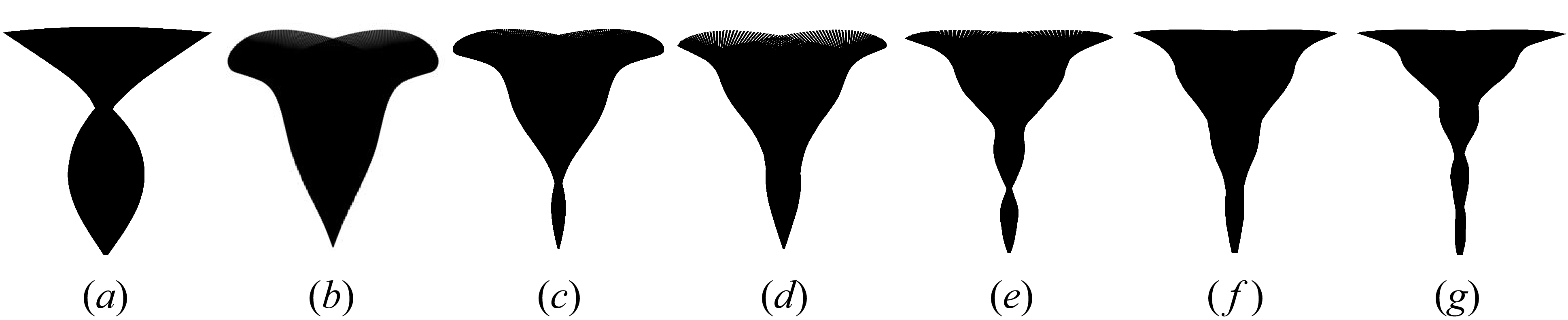
 (a)
 2
 (b)
 2+3
 (c)
 3
 (d)
 3+4
 (e)
 4
 (f)
 4+5
 (g)
 5

 Ms−KB
 (a)
 ReL=200
 (b)
 ReL=1000
 ∙
 2
 2+3
 3
 3+4
 4
 4+5
 5
 kz
 2π
 3π
 4π
 5π
 kz=2π

 Ms
 KB
 (a)
 ReL=200
 (b)
 ReL=1000
 y
 z

 A/L
 Ms
 KB
 (a)
 ReL=200
 (b)
 ReL=1000

 StL
 Ms
 KB
 (a)
 ReL=200
 (b)
 ReL=1000

 (a)
 (b)
 ReL=200
 ReL=1000

 (a)
 ReL=200
 (b)
 ReL=1000

 StL
 Ms
 (a)
 ReL=200
 (b)
 ReL=1000
 StL∼Ms−1/2
 KB
 StLMs∼KB1/2

 ReL=1000
 Ms
 KB

 ΔyRMSavg
 (a)
 ReL=200
 (b)
 ReL=1000

 (a)
 ReL=200
 (b)
 ReL=1000

 Ms−KB
 (a)
 ReL=200
 (b)
 ReL=1000

 Ms
 KB
 (a)
 ReL=200
 (b)
 ReL=1000

 ReL=1000
 Ms=2
 KB=3×10⁻²
 Q
 Q=0.1(U/L)2

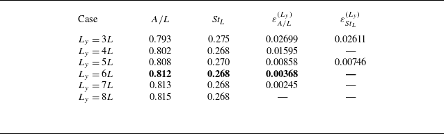
 Ly
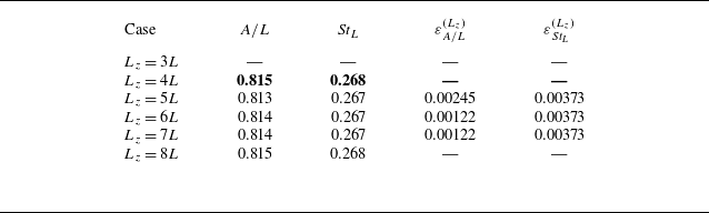
 Lz
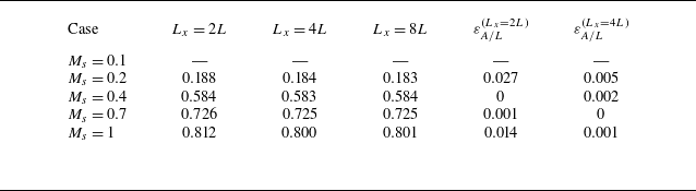
 Lx=2L,4L
 8L
 ReL=200
 Lx=2L
 Lx=4L
 Lx=8L
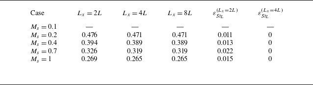
 Lx=2L,4L
 8L
 ReL=200
 Lx=2L
 Lx=4L
 Lx=8L
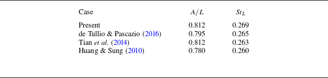
 ReL=200
 Ms=1
 KB=10−4
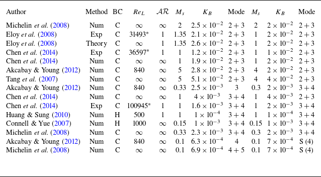
 Ms
 KB
 Ms
 KB
 ReL=1000
 KB
 KB
 ∗

 Open access

