1 Introduction
In this paper, we address the following family of questions which relate dynamics to topology for a pseudo-Anosov flow
 $\varphi $
in a 3-manifold. Given a properly embedded surface S which is positively transverse to
 $\varphi $
, one can attempt to count orbits with respect to the intersection number with S. That is, one can consider the growth rate:
 $$ \begin{align*} \mathrm{gr}_{\varphi}(S) = \lim_{L\to \infty} \#\{\gamma:\gamma\cdot S \le L\}^{1/L}, \end{align*} $$
where
 $\gamma $
varies over closed orbits of
 $\varphi $
. If S is a cross section of
 $\varphi $
(that is, S intersects every flow line), then
 $\varphi $
is the suspension flow of a fibration with fiber S, and
 $\mathrm {gr}_{\varphi }(S)$
is the Teichmüller dilatation of the monodromy map (its logarithm is the entropy). If S is not a cross section, then this growth rate is
 $\infty $
, but we can interrogate the finer structure of
 $\varphi $
by considering
 $\varphi |S$
, the flow restricted to the complement of S. Growth rates of closed orbits in
 $\varphi |S$
can be counted with respect to their intersection with transverse surfaces in the complement of S, or more generally with respect to cohomology classes positive on the closed orbits of
 $\varphi |S$
.
Our main tool for studying these questions is the veering triangulation of Agol–Guéritaud, which is a canonical ideal triangulation associated to a pseudo-Anosov flow without perfect fits (see §4 for details on this condition and the Agol–Guéritaud construction). In a previous work [Reference Landry, Minsky and TaylorLMT20], we associated to such a triangulation an invariant called the veering polynomial and a transverse graph called the flow graph. In this paper, we will show that the triangulation parameterizes transverse surfaces, the flow graph gives an explicit coding for the flow, and the polynomial computes the growth rates.
In the case of a fibered manifold with pseudo-Anosov monodromy, the veering polynomial recovers McMullen’s Teichmüller polynomial, and the growth rates correspond to Teichmüller dilatations in the fibered cone of Thurston’s norm on homology. However, even in this case, we obtain some new information on the behavior of these dilatations—see Theorem E.
What arises from this, we hope, is evidence that the veering triangulation is an effective combinatorial tool for studying pseudo-Anosov flows, providing as it does an explicit coding which is sensitive simultaneously to the dynamics of the flow and the topology of the 3-manifold.
1.1 Growth rates
To summarize our results, we introduce the terminology in more detail. Let
 $\overline M$
be a closed oriented
 $3$
-manifold and let
 $\varphi $
be a pseudo-Anosov flow on
 $\overline M$
without perfect fits (see §4). We assume throughout that
 $\varphi $
has at least one singular orbit; that is,
 $\varphi $
is not Anosov. Let M denote
 $\overline M$
minus the singular orbits of
 $\varphi $
. Let
 $\tau $
be the veering triangulation of M dual to
 $\varphi $
furnished by the Agol–Guéritaud construction (Theorem 4.7).
The 2-skeleton
 $\tau ^{(2)}$
has the structure of an oriented branched surface and we can consider surfaces S carried by it. For such a surface, let
 $M|S$
denote M cut along S, and let
 $\varphi |S$
denote the restricted flow in
 $M|S$
, which is a semiflow in the sense of Fenley–Mosher [Reference Fenley and MosherFM01]. Assume for simplicity that S, and hence
 $M|S$
, is connected.
Let
 $\mathcal O_{\varphi }$
denote the closed orbits of
 $\varphi $
and
 $\mathcal O_{\varphi }|S$
those closed orbits that avoid S. We say that a cohomology class
 $\xi \in H^1(M|S)$
is positive if it is positive on orbits in
 $\mathcal O_{\varphi }|S$
as well as on certain peripheral ‘prong curves’ corresponding to the removed singular orbits (see §7 for details).
The veering polynomial
 $V_{\tau }$
previously defined in [Reference Landry, Minsky and TaylorLMT20] is an element of the group ring
 $\mathbb {Z}[H_1(M;\mathbb {Z})/\mathrm {torsion}]$
. We will define an adapted polynomial
 $V_{\varphi |S}$
in
 $\mathbb {Z}[H_1(M|S;\mathbb {Z})/\mathrm {torsion}]$
, morally obtained by deleting certain terms from
 $V_{\tau }$
(see §7.4 for the precise definition). A positive class
 $\xi \in H^1(M|S)$
gives rise to a specialization
 $V_{\varphi |S}^{\xi }(u)$
in the sense of McMullen (see §2.3), which is a single variable polynomial-like expression. Our main theorem about growth rates is the following.
Theorem A. (Growth rates of closed orbits)
Let S be a connected surface carried by
 $\tau ^{(2)}$
. Then for any positive class
 $\xi \in H^1(M|S)$
, the growth rate
 $$ \begin{align} \mathrm{gr}_{\varphi|S}(\xi) = \lim_{L\to \infty} \# \{ \gamma \in \mathcal O_{\varphi}|S : \xi(\gamma) \le L \} ^{{1}/{L}} \end{align} $$
exists and is equal to the reciprocal of the smallest positive root of the specialization
 $V_{\varphi |S}^{\xi }(u)$
of the veering polynomial at
 $\xi $
.
Moreover,
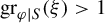 $\mathrm {gr}_{\varphi |S}(\xi )>1$
if and only if there are infinitely many closed primitive orbits of
 $\varphi $
that miss S.
See Theorem 7.2 for the general statement, in particular allowing disconnected S.
Remark 1.1. Using Corollary 9.8 and code written by Parlak, Schleimer, and Segerman [Reference Parlak, Schleimer and SegermanPSS22], Ross Griebenow has found explicit examples of surfaces S carried by
 $\tau ^{(2)}$
missing infinitely many closed primitive orbits of
 $\varphi $
[Reference GriebenowGri22]. Hence,
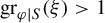 $\mathrm {gr}_{\varphi |S}(\xi )>1$
for such examples by Theorem A.
In fact, in the forthcoming paper [Reference Landry, Minsky and TaylorLMT22], we give a construction which shows that such examples are plentiful. Starting with a general type of endperiodic map on an infinite-type surface, we produce a surface S in a fibered manifold M with a pseudo-Anosov suspension flow
 $\varphi $
. The infinite-type surface determines a class
 $\xi \in H^1(M|S)$
, and the growth rate
 $\mathrm {gr}_{\varphi |S}(\xi )$
is the ‘stretch factor’ of the original endperiodic map. See Remark 9.9 for some details on the connection between growth rates and stretch factors. It is then easy to produce endperiodic maps so that the associated stretch factors are greater than 1.
Let
 ${\mathcal C}^+$
be the cone in
 $H^1(M|S)$
consisting of positive classes. The associated entropy function is
 $$ \begin{align*} \mathrm{ent}_{\varphi|S} :\, &{\mathcal C}^+ \to [0, \infty)\\ &\xi \mapsto \log(\mathrm{gr}_{\varphi|S}(\xi)), \end{align*} $$
where
 $\mathrm {gr}_{\varphi |S}$
is given by equation (1.1). The following result, which is a combination of Theorem 9.1 and Theorem 9.3, establishes the essential properties of the entropy function on the cone of positive classes. In §9.1, we define what it means for the restricted semiflow to be essentially transitive and refer the reader there for details.
Theorem B. (Entropy)
The entropy function
 $\mathrm {ent}_{\varphi |S} : {\mathcal C}^+ \longrightarrow [0,\infty )$
is continuous, convex, and homogeneous of degree
 $-1$
.
Moreover, if the semiflow
 $\varphi |S$
is essentially transitive, then
 $\mathrm {ent}_{\varphi |S}$
is real analytic, strictly convex, and blows up at the boundary of
 ${\mathcal C}^+$
.
Throughout this discussion, we have focused on the manifold M. However, much of this theory extends to study transverse surfaces in the original closed manifold
 $\overline M$
. See, for example, Theorem 8.1 which is an analogue of Theorem A for transverse surfaces in
 $\overline M$
.
1.2 Transversality and coding
Theorems A and B rely on the following results which connect the flow to the combinatorial structure of
 $\tau $
and its flow graph.
Theorem C. (Transversality)
The veering triangulation
 $\tau $
dual to
 $\varphi $
can be realized in M so that the cooriented branched surface
 $\tau ^{(2)}$
is positively transverse to the flow lines of
 $\varphi $
.
While this transversality is automatic in the setting of a suspension flow, the general case requires a surprisingly delicate argument. For a more detailed statement, see Theorem 5.1.
One important takeaway from Theorem C is that surfaces that are carried by
 $\tau ^{(2)}$
, which are often in plentiful supply, are automatically transverse to the flow
 $\varphi $
. For example, by Theorem 2.2, any class in
 $H^1(M)$
that is non-negative on closed positive transversals of
 $\tau ^{(2)}$
is represented by a surface carried by
 $\tau ^{(2)}$
and such classes form the entire cone over a face of the Thurston norm ball.
In [Reference Landry, Minsky and TaylorLMT20], we used the combinatorial structure of
 $\tau $
to define a directed graph
 $\Phi $
, called the flow graph of
 $\tau $
, and an embedding
 $\iota : \Phi \to M$
which maps edges of
 $\Phi $
to arcs that are positively transverse to
 $\tau ^{(2)}$
. The next result (which is a summary of facts stated in Theorem 6.1 and Proposition 6.12) justifies the name flow graph by establishing that
 $\Phi $
codes the orbits of
 $\varphi $
.
Theorem D. (Coding
 $\varphi $
with
$\Phi $
)


The map
 $\iota : \Phi \to M$
establishes a correspondence between directed lines in
 $\Phi $
and flow lines in
 $\overline M$
, which is surjective and uniformly bounded-to-one.
Restricting this correspondence to closed directed cycles, we get a one-to-one correspondence with the exception of finitely many orbits and their positive multiples.
In fact, we can say far more about the correspondence between closed directed cycles of
 $\Phi $
and closed orbits of
 $\varphi $
. See Theorem 6.1 for the detailed statement. The upshot is that the explicit coding of the flow
 $\varphi $
by the flow graph
 $\Phi $
allows us to address Theorems A and B using tools from the study of growth rates of directed cycles of graphs, as in McMullen’s work on the clique polynomial [Reference McMullenMcM15].
1.3 Fibered faces and stretch factors
Let us recall some of the theory developed for fibered manifolds by Thurston [Reference ThurstonThu86], Fried [Reference FriedFri79, Reference FriedFri82b], and McMullen [Reference McMullenMcM00], which motivates most of our results.
Thurston defined a norm on the vector space
 $H^1(\overline M;\mathbb {R})$
of a 3-manifold whose unit ball B is a polyhedron, and which organizes the fibrations of
 $\overline M$
over the circle in the following sense: Any integral class
 $\alpha \in H^1(\overline M;\mathbb {Z})$
which is Poincaré dual to the fiber of a fibration must appear in the cone
 $\mathbb {R}_+\textbf {F}$
on an open top-dimensional face
 $\textbf {F}$
of B, and, moreover, all other integral points of this cone correspond to fibers as well (hence
 $\textbf {F}$
is called a fibered face, and
 $\alpha $
a fibered class).
Further, the suspension flows associated to the various fibers in the cone
 $\mathbb {R}_+\textbf {F}$
agree, up to isotopy and reparameterization, and so we identify them with a single circular flow
 $\varphi $
. Here a flow is circular if it admits a cross section and so is, up to reparameterization, a suspension flow.
The orbit growth rate
 $\mathrm {gr}_{\varphi }(\alpha )$
defined above, can also be interpreted as the stretch factor, or Teichmüller dilatation, of the return map of the flow to a fiber associated to
 $\alpha $
. Its logarithm, the entropy of the return map, extends to a function
 $h_{\varphi } : \mathbb {R}_+\mathrm {int}(\textbf {F}) \to (0, \infty )$
that is continuous, convex, and blows up at the boundary of
 $\mathbb {R}_+\textbf {F}$
[Reference FriedFri82a, Theorem E]. McMullen extends Fried’s result by showing that
 $h_{\varphi }$
is additionally real analytic and strictly convex [Reference McMullenMcM00, Corollary 5.4]. To do so, he introduced a new polynomial invariant, called the Teichmüller polynomial, which both packages growth rates of the flow and detects the fibered cone
 $\mathbb {R}_+\textbf {F}$
in a precise sense. Since McMullen’s work, the Teichmüller polynomial has become a central tool in the study of these stretch factors; see e.g. [Reference HironakaHir10, Reference Kin, Kojima and TakasawaKKT13, Reference Leininger and MargalitLM13, Reference SunSun15].
The veering polynomial is a direct generalization of the Teichmüller polynomial, with Theorem A extending McMullen’s theorem on growth rates and Theorem B extending the theorem on the properties of
 $h_{\varphi }$
.
Now suppose
 $\xi $
is a fibered class, while S is a surface transverse to
 $\varphi $
which is not a fiber. Then
 $\xi $
pulls back to a positive class in
 $H^1(M|S)$
in the sense of Theorem A, and
 $\mathrm {gr}_{\varphi |S}(\xi )$
can be interpreted as both the growth rate with respect to
 $\xi $
of closed orbits of
 $\varphi $
that miss S (Corollary 9.8) as well as the stretch factor of an endperiodic homeomorphism of the infinite type surface obtained by ‘spinning’ the fiber representatives of
 $\xi $
around S (Remark 9.9). In fact, these quantities all arise as accumulation points of the set of stretch factors of pseudo-Anosov return maps to fibers in
 $\mathbb {R}_+\textbf {F}$
.
To be more precise, let
 $\Lambda _{\textbf {F}}\subset [1,\infty )$
be the set of stretch factors of monodromies associated to fibers in
 $\mathbb {R}_+\textbf {F}$
and let
 $\overline \Lambda _{\textbf {F}}$
be its closure. Denote by
 $\overline \Lambda _{\textbf {F}}'$
its derived set (that is, set of limit points) and set
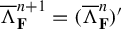 $\overline \Lambda _{\textbf {F}}^{n+1} = (\overline \Lambda _{\textbf {F}}^{n}) '$
. The following theorem answers a question of Chris Leininger (see Question 1).
Theorem E. (Stretch factors and fibered cones)
The stretch factor set
 $\overline \Lambda _{\textbf {F}}$
is compact, well-ordered under
 $\ge $
, and
 $\overline \Lambda _{\textbf {F}}^n = \{1 \}$
for some
 $1\le n \le \mathrm {dim}(H^1(M;\mathbb {R})$
.
A more detailed statement can be found in Theorem 9.10, including the relation between limit points of
 $\Lambda _{\textbf {F}}$
and growth rates of the form
 $\mathrm {gr}_{\varphi |S}(\xi )$
.
1.4 Connections to previous and ongoing wor
Although Agol and Guéritaud’s construction of a veering triangulation from a pseudo-Anosov flow without perfect fits is unpublished, there are many established connections between veering triangulations and the topology, geometry, and dynamics of their underlying manifolds. These include links to pseudo-Anosov stretch factors [Reference AgolAgo11], angle structures [Reference Futer and GuéritaudFG13, Reference Hodgson, Hyam Rubinstein, Segerman and TillmannHRST11], hyperbolic geometry [Reference Futer, Taylor and WordenFTW20, Reference GuéritaudGué16, Reference Hodgson, Issa and SegermanHIS16], and the curve complex [Reference Minsky and TaylorMT17, Reference StrennerStr18].
More relevant to this paper is the work of Landry [Reference LandryLan18, Reference LandryLan19, Reference LandryLan22], which studies the surfaces carried by the underlying
 $2$
-skeleton of the veering triangulation. This connects to our previous work [Reference Landry, Minsky and TaylorLMT20] introducing the veering polynomial, relating it to the Teichmüller polynomial, and laying the combinatorial groundwork for what is done here (although we emphasize that this paper can be read independently of the previous). Also, Parlak has recently introduced and implemented algorithms to compute the veering polynomial and its relatives [Reference ParlakPar21a], and demonstrated a connection with the Alexander polynomial [Reference ParlakPar21b], thereby generalizing the work of McMullen on the Teichmüller polynomial [Reference McMullenMcM00].
Finally, the Agol–Guéritaud construction is expected to be reversible in the sense that a veering triangulation should determine a pseudo-Anosov flow and the process of going from one to the other should be inverse operations. Proving this statement is an ongoing program of Schleimer–Segerman, the first part of which is [Reference Schleimer and SegermanSS19] where from a veering triangulation, a combinatorial ‘flow space’ is reconstructed. There is also forthcoming work of Agol–Tsang [Reference Agol and TsangAT21], which produces a pseudo-Anosov flow from a veering triangulation, but without the claim that it is canonical or that it recovers the original flow if the veering triangulation was produced by the Agol–Guéritaud construction.
1.5 Outline of paper
In §2, we review essential properties of veering triangulations as well as some basic structure we introduced in [Reference Landry, Minsky and TaylorLMT20]. This is followed by §3 which lays out one of our primary combinatorial tools, which we call dynamic planes.
Background on pseudo-Anosovs flows and the construction of Agol–Guéritaud, which builds the dual veering triangulation, is presented in §4. In §5, we prove Theorem C that the veering triangulation can be realized positively transverse to
 $\varphi $
, and §6 uses this transversality to prove Theorem D that the flow graph codes the orbits of
 $\varphi $
. Theorem A is then a consequence of these results along with connection between dynamic planes and the flow space of
 $\varphi $
, as established in §7.
In §8, we prove a version of Theorem A that covers the case of closed surfaces transverse to the flow
 $\varphi $
on the closed manifold
 $\overline M$
. In this section, the veering triangulation only appears as a tool in the proof. Finally, in §9, we give several applications of our main theorems. These include Theorems B and E.
2 The flow graph, the veering polynomial, and carried surfaces
Here we record some required background and summarize results from our previous work [Reference Landry, Minsky and TaylorLMT20]. Background on pseudo-Anosov flows will be deferred until §4.
2.1 Veering triangulations
A veering triangulation of a
 $3$
-manifold M is a taut ideal triangulation together with a coherent assignment of veers to its edges. We begin by explaining each of these terms.
A taut ideal tetrahedron is an ideal tetrahedron (that is, a tetrahedron without vertices) along with a coorientation on each face so that it has two inward pointing faces, called its bottom faces, and two outward pointing faces, called its top faces. Each of its edges is then assigned either angle
 $\pi $
or
 $0$
depending on whether the coorientations on the adjacent faces agree or disagree, respectively.
Following Lackenby [Reference LackenbyLac00], an ideal triangulation of M is taut if each of its faces has been cooriented so that each ideal tetrahedron is taut and the angle sum around each edge is
 $2\pi $
. The local structure around each edge
 $\textit {e}$
is as follows:
 $\textit {e}$
includes as a
 $\pi $
-edge into two tetrahedra. For the other tetrahedra meeting
 $\textit {e}$
,
 $\textit {e}$
includes as an
 $0$
-edge and these tetrahedra are divided into the two sides, called fans of
 $\textit {e}$
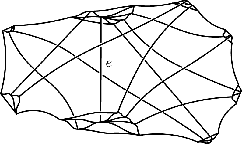
, each of which is linearly ordered by the coorientation on faces. The length of each fan is one less than the degree of e on that side. See Figure 1.
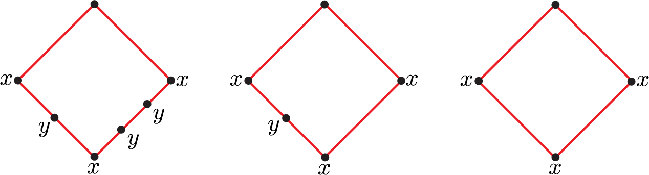
The edge e has one fan of length 1 and one fan of length 3.

A veering triangulation
 $\tau $
of M is a taut ideal triangulation of M in which each edge has a consistent veer. This means that each edge is labeled to be either right or left veering such that each tetrahedron of
 $\tau $
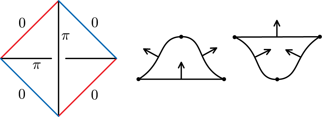
admits an orientation-preserving isomorphism to the model veering tetrahedron pictured in Figure 2, in which the veers of the 0-edges are specified: right veering edges have positive slope and left veering edges have negative slope. The
 $\pi $
-edges can veer either way, as long as adjacent tetrahedra satisfy the same rule. If the
 $\pi $
-edges of a tetrahedron have opposite veer, the tetrahedron is said to be hinge; otherwise it is non-hinge.
A model veering tetrahedron and its cusps with their coorientations (in colour online).

2.2 The dual graph, flow graph, and stable branched surface
The stable branched surface
 $B^s$
in M associated to the veering triangulation
 $\tau $
, introduced in [Reference Schleimer and SegermanSS19] as the upper branched surface in dual position and in [Reference Landry, Minsky and TaylorLMT20, §4], plays a central role throughout this paper. We refer the reader to [Reference Floyd and OertelFO84, Reference OertelOer84] for general facts about branched surfaces.
Topologically, the stable branched surface
 $B^s$
is the dual complex of
 $\tau $
in M, and as such, it is a deformation retract of M. Note that
 $B^s$
is two-dimensional since
 $\tau $
has no vertices. For each tetrahedron t, we define a smooth structure on
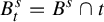 $B^s_t = B^s \cap t$
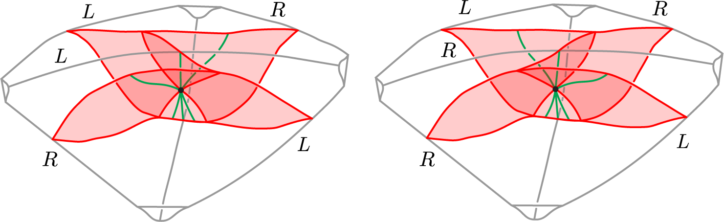
as follows: if the top edge of t is left veering, then we smooth according to the left-hand side of Figure 3 and otherwise we smooth according the the right-hand side. It is proven in [Reference Landry, Minsky and TaylorLMT20, Lemma 4.3] that this produces a well-defined global smooth structure making
 $B^s$
into a branched surface.
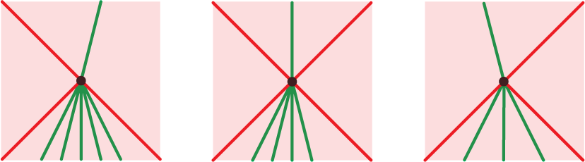
The stable branched surface
 $B^s$
within a single tetrahedron. Its intersection with the flow graph, where edges are directed upward, is shown in green (note: the number of incoming edges at a vertex may vary) (in colour online).

The stable branched surface contains two directed graphs related to
 $\tau $
that are also of central importance. The first, is the dual graph
 $\Gamma $
of
 $\tau $
which is defined to be the
 $1$
-skeleton of
 $B^s$
whose edges are directed by the coorientation on the faces of
 $\tau $
. Alternatively,
 $\Gamma $
is the graph with a vertex interior to each tetrahedron and a directed edge crossing each cooriented face from the vertex in the tetrahedron below the face to the vertex in the tetrahedron above the face. See Figure 3. The directed cycles of
 $\Gamma $
are called dual cycles or
 $\Gamma $
-cycles. Here and throughout, a directed cycle of a directed graph is an oriented loop determined by a cyclic concatenation of directed edges.
As the
 $1$
-skeleton of the branched surface
 $B^s$
, each turn in the graph
 $\Gamma $
is either branching, that is, realized by a smooth arc in
 $B^s$
, or else what we call anti-branching (or AB). In greater detail, a turn of
 $\Gamma $
is an ordered pair
 $(e_1,e_2)$
of directed
 $\Gamma $
-edges so that the terminal vertex v of
 $e_1$
equals the initial vertex of
 $e_2$
. The turn is branching if the arc
 $e_1 \cup e_2$
is smooth as an arc in the singular locus of
 $B^s$
and is anti-branching (or AB) otherwise. A directed path, ray, or cycle in
 $\Gamma $
that makes only branching turns is called a branch path, ray, or cycle, respectively. Similarly, a directed path, ray, or cycle in
 $\Gamma $
that makes only AB turns is called an AB path, ray, or cycle. We note that since for each vertex of
 $\Gamma $
each incoming edge is part of exactly one branching turn and one AB turn, there are only finitely many branch and AB cycles in
 $\Gamma $
.
Branching and anti-branching turns of
 $\Gamma $
can be characterized solely in terms of the veering combinatorics [Reference Landry, Minsky and TaylorLMT20, Lemma 4.5] and from this we can deduce a few important properties of the sectors of
 $B^s$
.
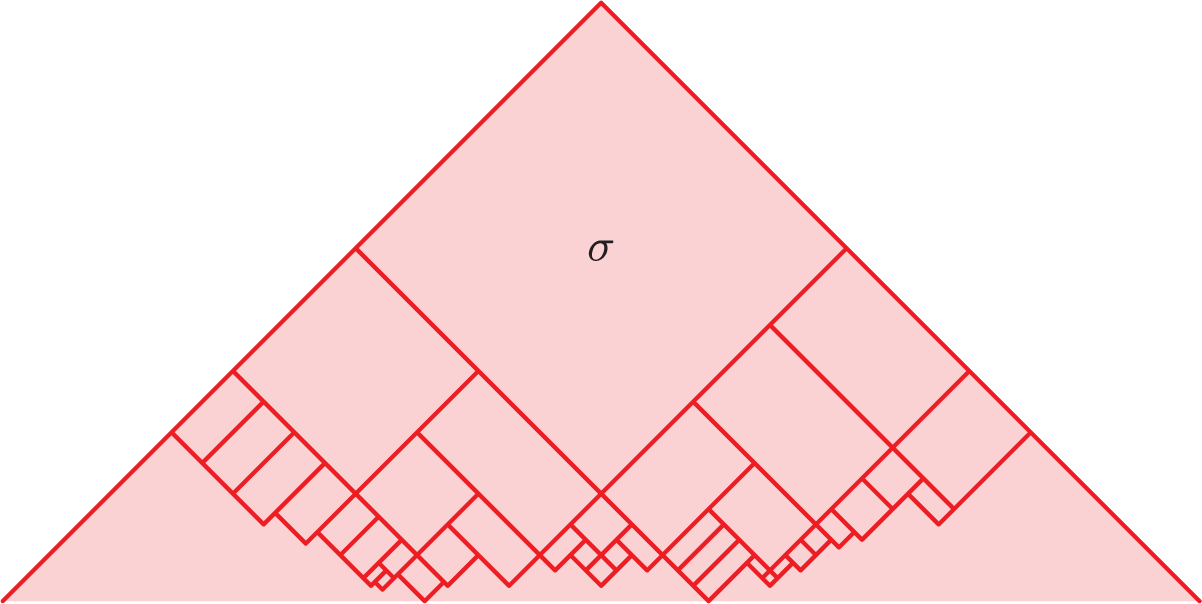
Each sector
 $\sigma $
of
 $B^s$
is a topological disk pierced by a single
 $\tau $
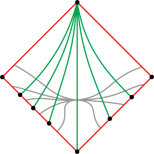
-edge, as in Figure 4. The
 $\Gamma $
-edges bounding
 $\sigma $
are oriented so that exactly one vertex is a source, which we call the bottom of
 $\sigma $
, and one is a sink, which we call the top of
 $\sigma $
. The top and bottom divide the boundary of
 $\sigma $
into two oriented
 $\Gamma $
-paths called sides. Each side has at least two
 $\Gamma $
-edges because the
 $\tau $
-edge piercing
 $\sigma $
has a non-empty fan on each side. According to the following lemma, which appears as [Reference Landry, Minsky and TaylorLMT20, Lemma 4.6], if you remove the last edge in any side of any sector of
 $B^s$
, the resulting path is a branch segment, and the entire side is never a branch segment. See Figure 4, where the AB turns appear as corners of the sector. We call these vertices the corner vertices of the sector.
A sector of
 $B^s$
and its intersection with
 $\Phi $
(green) and
 $\tau ^{(2)}$
(gray). The triple points of
 $B^s$
, which are the vertices of
 $\Gamma $
and
 $\Phi $
, are in black. All edges are directed upward; the top is the northmost vertex, the bottom is the southmost, and the corners are westmost/eastmost (in colour online).

Lemma 2.1. (Sectors and turns)
Let
 $\sigma $
be a sector of
 $B^s$
and let p be a side of
 $\sigma $
considered as a directed path in
 $\Gamma $
from the bottom to the top of
 $\sigma $
. The last turn of p is anti-branching, and all other turns are branching.
The second directed graph embedded in
 $B^s$
is the flow graph
 $\Phi $
of
 $\tau $
, which was introduced in [Reference Landry, Minsky and TaylorLMT20, §4.3]. The vertices of
 $\Phi $
are in correspondence with
 $\tau $
-edges, and for each tetrahedron t of
 $\tau $
, there are
 $\Phi $
-edges from the bottom
 $\tau $
-edge of each tetrahedron to its top
 $\tau $
-edge and the two side
 $\tau $
-edges whose veer is opposite that of the top
 $\tau $
-edge.
This defines
 $\Phi $
as an abstract directed graph, but it also comes equipped with an embedding
 $\iota : \Phi \to B^s$
, which was called dual position in [Reference Landry, Minsky and TaylorLMT20]. Each
 $\tau $
-edge e is at the bottom of a unique tetrahedron
 $t_e$
and
 $\iota $
maps the vertex of
 $\Phi $
corresponding to e to the vertex of
 $\Gamma $
contained in
 $t_e$
. Each directed edge of
 $\Phi $
is then mapped into a single sector of
 $B^s$
so that it is positively transverse to
 $\tau ^{(2)}$
. See Figure 3. According to [Reference Landry, Minsky and TaylorLMT20, Lemma 4.7], for each sector
 $\sigma $
of
 $B^s$
, there is a directed edge of
 $\iota (\Phi ) \cap \sigma $
coming into the top vertex of
 $\sigma $
from each vertex of
 $\sigma $
other than its two corner vertices. See Figure 4. This characterizes the flow graph in dual position according to its intersection with each sector of
 $B^s$
.
The directed cycles of
 $\Phi $
, along with their images under
 $\iota $
, are called flow cycles or
 $\Phi $
-cycles. When convenient, we sometimes identify
 $\Phi $
with its image under
 $\iota $
.
2.3 The veering polynomial
Fix a finitely generated, free abelian group G and denote its group ring with integer coefficients by
 $\mathbb {Z}[G]$
. Let
 $P \in \mathbb {Z}[G]$
and write
 $P= \sum _{g\in G} a_g \cdot g$
. The support of P is
 $$ \begin{align*} \mathrm{supp}(P) = \{g \in G : a_g \neq 0 \}. \end{align*} $$
For
 $P \in \mathbb {Z}[G]$
with
 $P = \sum _{g\in G} a_g \cdot g$
and
 $\alpha \in \mathrm {Hom}(G,\mathbb {R})$
, the specialization of P at
 $\alpha $
is the single variable expression
 $P^{\alpha }$
in
 $\mathbb {Z}[u^r : r \in \mathbb {R}]$
given by
 $$ \begin{align*} P^{\alpha}(u) = \sum_{g\in G} a_g \cdot u^{\alpha(g)}. \end{align*} $$
These generalities will be used in the specific setting of veering polynomials. For this, let M be a
 $3$
-manifold with veering triangulation
 $\tau $
, and set
 $G = H_1(M;\mathbb {Z})/\mathrm {torsion}$
. In [Reference Landry, Minsky and TaylorLMT20, §2], we defined a polynomial invariant
 $V_{\tau } \in \mathbb {Z}[G]$
, called the veering polynomial of
 $\tau $
. Here, we recall an alternative characterization of
 $V_{\tau }$
in terms of the Perron polynomial of the flow graph
 $\Phi $
. We refer the reader to [Reference Landry, Minsky and TaylorLMT20, §4] for additional details.
For a directed graph D, let A denote the matrix with entries
 $$ \begin{align} A_{ab} = \sum_{\partial e=b-a} e, \end{align} $$
where the sum is over all edges e from the vertex a to the vertex b. We call A the adjacency matrix for D. The Perron polynomial of D is defined to be
 $P_D = \det (I - A)$
. By definition, this is an element of
 $\mathbb {Z}[C_1(D)]$
, where
 $C_1(D)$
is the group of simplicial 1-chains in D.
Following McMullen [Reference McMullenMcM15], we define the cycle complex
 $\mathcal {C}(D)$
of D to be the graph whose vertices are directed simple cycles of D and whose edges correspond to disjoint cycles. We recall that
 $P_D$
equals the clique polynomial of
 $\mathcal {C}(D)$
, which in particular shows that
 $P_D$
is an element of the subring
 $\mathbb {Z}[H_1(D)]$
(see [Reference McMullenMcM15, Theorem 1.4 and §3]). Here, the clique polynomial associated to
 $\mathcal {C}(D)$
is
 $$ \begin{align} P_D = 1 + \sum_{C} (-1)^{|C|} C \in \mathbb{Z}[H_1(D)], \end{align} $$
where the sum is over non-empty cliques C of the graph
 $\mathcal {C}(D)$
, that is, over simple multicycles of D, and
 $|C|$
is the number of vertices of C, that is, the number of components of the multicycle. Note that the support of P is the set
 $\mathrm {supp}(P_D) = \{ C\} \subset H_1(D)$
of directed simple multicycles appearing in equation (2.2).
Now let
 $\iota : \Phi \to M$
be the flow graph with its embedding into M. This induces a ring homomorphism
 $\iota _*: \mathbb {Z}[H_1(\Phi )] \to \mathbb {Z}[G]$
and we set
 $$ \begin{align*} V_{\tau} = \iota_*(P_{\Phi}), \end{align*} $$
where
 $P_{\Phi }$
is the Perron polynomial of
 $\Phi $
. According to [Reference Landry, Minsky and TaylorLMT20, Theorem 4.8], this agrees with the original definition of the veering polynomial.
2.4 Surfaces carried by
$\tau $
and cones in (co)homology

As noted by Lackenby [Reference LackenbyLac00], tautness of
 $\tau $
naturally gives its
 $2$
-skeleton
 $\tau ^{(2)}$
the structure of a transversely oriented branched surface in M. The smooth structure on
 $\tau ^{(2)}$
can be obtained by, within each tetrahedron, smoothing along the
 $\pi $
-edges and pinching along the
 $0$
-edges, thus giving
 $\tau ^{(2)}$
a well-defined tangent plane field at each of its points.
As a transversely oriented branched surface,
 $\tau ^{(2)}$
can carry surfaces similarly to the way a train track on a surface can carry curves. We let
 $\mathrm {cone}_2(\tau )$
be the closed cone in
 $H_2(M,\partial M)$
positively generated by classes that are represented by the surfaces that
 $\tau $
carries. We call
 $\mathrm {cone}_2(\tau )$
the cone of carried classes.
In a bit more detail, the branched surface
 $\tau ^{(2)}$
has a branched surface fibered neighborhood
 $N= N(\tau ^{(2)})$
foliated by intervals such that collapsing N along its I-fibers recovers
 $\tau ^{(2)}$
. The transverse orientation on the faces of
 $\tau $
orients the fibers of N, and a properly embedded oriented surface S in M is carried by
 $\tau ^{(2)}$
if it is contained in N where it is positively transverse to its I-fibers. We also say that S is carried by
 $\tau $
.
A carried surface S embedded in N transverse to the fibers defines a non-negative integral weight on each face of
 $\tau $
given by the number of times the I-fibers over that face intersect S. These weights satisfy the matching (or switch) conditions stating that the sum of weights on one side of an edge match the sum of weights on the other side. Conversely, a collection of non-negative integral weights satisfying the matching conditions gives rise to a surface embedded in N transverse to the fibers in the usual way. More generally, any collection of non-negative weights on faces of
 $\tau $
satisfying the matching conditions defines a non-negative relative cycle giving an element of
 $H_2(M, \partial M; \mathbb {R})$
and we say that a class is carried by
 $\tau ^{(2)}$
if it can be realized by such a non-negative cycle. Hence,
 $\mathrm {cone}_2(\tau )$
is precisely the subset of
 $H_2(M,\partial M)$
consisting of carried classes.
The following theorem is a summary of results in [Reference Landry, Minsky and TaylorLMT20, Theorems 5.1 and 5.12]. For its statement, we let
 $\mathrm {cone}_1(\Gamma ) \subset H_1(M; \mathbb {R})$
denote the cone positively spanned by the direct cycles of the dual graph
 $\Gamma $
. We call
 $\mathrm {cone}_1(\Gamma )$
the cone of homology directions of
 $\tau $
and note that it is equal to the cone positively generated by all closed curves which are positively transverse to
 $\tau ^{(2)}$
at each point of intersection. We write
 $\mathrm {cone}_1^{\vee }(\Gamma )$
for its dual cone in
 $H^1(M; \mathbb {R})$
, which consists of classes that are non-negative on all dual cycles.
Theorem 2.2. (Cones and Thurston norm)
For any veering triangulation
 $\tau $
of M, the following hold.
-
(1) The cone of homology directions
$\mathrm {cone}_1(\Gamma )$
is positively generated by
$\iota (\mathrm {supp}(P_{\Phi }))$
, the image of the support of
$P_{\Phi }$
. -
(2) After identifying
$H^1(M;\mathbb {R}) = H_2(M, \partial M; \mathbb {R})$
,
$\mathrm {cone}_2(\tau ) = \mathrm {cone}_1^{\vee }(\Gamma )$
. -
(3) There is a cone
$\mathbb {R}_+\textbf {F}_{\tau }$
over a (possibly empty) face
$\textbf {F}_{\tau }$
of the Thurston norm ball in
$H_2(M, \partial M)$
such that
$\mathrm {cone}_2(\tau ) = \mathbb {R}_+\textbf {F}_{\tau }$
.







So, for example, a class
 $\alpha \in H_2(M,\partial M)$
is carried by
 $\tau $
if and only if
 $\langle \alpha , \iota (c) \rangle \ge 0$
for each simple directed cycle c of
 $\Phi $
.
3 Dynamic planes and flow cycles
In this section, we introduce and develop the essential features of dynamic planes of the veering triangulation
 $\tau $
. A dynamic plane is a combinatorial version of a leaf of the weak stable foliation of a pseudo-Anosov flow but with additional structure coming from its interaction with the dual and flow graphs of
 $\tau $
. The main results are Proposition 3.15, which says that all but finitely many dual cycles (and their multiples) are homotopic to flow cycles, and Lemma 3.17, which combinatorially characterizes when dual cycles are homotopic within the quotient of a dynamic plane. Both these technical facts will be essential in §6 where we describe precisely how the flow graph codes the orbits of the dual flow.
3.1 Descending sets and dynamic planes
For any branched surface B, let
 $N(B)$
denote a regular neighborhood of B foliated in the standard way by intervals. Let
 $$ \begin{align*} \operatorname{\mathrm{coll}}: N(B)\twoheadrightarrow B \end{align*} $$
be the map which collapses all the intervals.
If B is a branched surface with generic branching, then we denote its branch locus, that is, its collection of non-manifold points, by
 $\operatorname {\mathrm {brloc}} (B)$
. The maw vector field is a vector field tangent to B defined on
 $\operatorname {\mathrm {brloc}} (B)$
that always points from the 2-sheeted side to the 1-sheeted side. Note that the maw vector field is defined even at triple points; see Figure 5.
The maw vector field (in colour online).

A descending path in B is an oriented immersed curve in B whose tangent vector at each point of intersection with
 $\operatorname {\mathrm {brloc}}(B)$
is equal to the maw vector field at that point.
We next consider the stable branched surface
 $B^s$
. Note that, up to homotopy, any closed descending path in
 $B^s$
is negatively transverse to
 $\tau ^{(2)}$
(see Figure 4), and is therefore homotopically non-trivial in M [Reference Schleimer and SegermanSS20, Theorem 3.2]. Let
 $\widetilde B^s$
,
 $\widetilde \Gamma $
, and
 $\widetilde \Phi $
be the preimages of
 $B^s$
,
 $\Gamma $
, and
 $\Phi $
, respectively, in the universal cover
 $\widetilde M$
of M.
Let
 $\sigma $
be a sector of the branched surface
 $\widetilde B^s$
. The descending set of
 $\sigma $
, denoted
 $\Delta (\sigma )$
, is defined to be the union of all sectors
 $\sigma '$
of
 $\widetilde B^s$
such that there exists a descending path from
 $\sigma $
to
 $\sigma '$
. Before describing
 $\Delta (\sigma )$
in detail, recall that by a path, ray, or line in
 $\Gamma $
or
 $\Phi $
, we always mean a directed path, ray, or line. If
 $\ell $
is a branch line in
 $\widetilde \Gamma $
through a vertex v, then the negative subray of
 $\ell $
at v is the portion of the branch line
 $\ell $
that lies below v.
Lemma 3.1. (Structure of
$\Delta (\sigma )$
)

Let
 $\sigma $
be a
 $\widetilde B^s$
-sector.
-
(a) The descending set
$\Delta (\sigma )$
is diffeomorphic to a closed quarter plane bounded by the negative subrays of the two branch lines passing through the top vertex v of
$\sigma $
. -
(b) If w is a
$\widetilde \Gamma $
-vertex contained in
$\Delta (\sigma )$
, then any
$\widetilde \Gamma $
-ray starting at w intersects
$\partial \Delta (\sigma )$
. -
(c) If w is a
$\widetilde \Gamma $
-vertex contained in
$\operatorname {\mathrm {int}}(\Delta (\sigma ))$
, there is a unique outgoing
$\widetilde \Phi $
-edge incident to w contained in
$\Delta (\sigma )$
. The unique
$\widetilde \Phi $
-ray starting at w lying in
$\Delta (\sigma )$
terminates on
$\partial \Delta (\sigma )$
.


Before the proof, let us establish a few facts that we will need. By [Reference Schleimer and SegermanSS19, Theorem 8.1], the branched surface
 $B^s$
fully carries a unique two-dimensional lamination
 $\mathcal L^s$
without parallel leaves such that
 $\mathcal L$
is essential and each leaf of
 $\mathcal L^s$
is either a plane, an
 $\pi _1$
-injective annulus, or a
 $\pi _1$
-injective Möbius band. Denote by
 $\widetilde {\mathcal L}^s$
the lamination lifted to the universal cover
 $\widetilde M$
whose leaves are planes. Note that since
 $\widetilde {\mathcal L}^s$
is carried by
 $\widetilde B^s$
, each leaf inherits a tessellation corresponding to the sectors of
 $\widetilde B^s$
it traverses.
It is clear from the branching structure of
 $B^s$
(cf. [Reference Schleimer and SegermanSS19, Remark 8.27]) that if
 $\ell $
is a leaf carried by
 $\widetilde B^s$
such that
 $\operatorname {\mathrm {coll}}(\ell )$
contains
 $\sigma $
, and if there is a descending path from
 $\sigma $
to another sector
 $\sigma '$
, then
 $\sigma '$
is also contained in
 $\operatorname {\mathrm {coll}}(\ell )$
. Consequently, we have that
 $\operatorname {\mathrm {coll}}(\ell )$
contains the descending set of every sector traversed by
 $\ell $
.
We also observe that each leaf of
 $\widetilde {\mathcal L}^s$
traverses a sector of
 $\widetilde B^s$
at most once. For if
 $\ell $
is a leaf traversing a sector
 $\sigma $
twice, a short segment contained in a regular neighborhood of
 $\sigma $
connecting two points of
 $\ell $
identified under
 $\operatorname {\mathrm {coll}}$
may be homotoped to lie entirely in
 $\ell $
. Since the branched surface
 $B^s$
is laminar (as observed in [Reference Schleimer and SegermanSS19]) and hence essential, this contradicts [Reference Gabai and OertelGO89, Theorem 1.d] (see also [Reference Gabai and OertelGO89, Lemma 2.7]). We conclude that for any leaf
 $\ell $
of
 $\widetilde {\mathcal L}^s$
,
 $\operatorname {\mathrm {coll}}(\ell )$
is a plane embedded in
 $\widetilde B^s\kern-1.2pt $
.
Proof of Lemma 3.1
We begin by using the above discussion to prove part (a). Let
 $\ell $
be any leaf of
 $\widetilde {\mathcal L}^s$
that traverses
 $\sigma $
. Then
 $P = \operatorname {\mathrm {coll}}(\ell )$
is a plane tessellated by sectors of
 $\widetilde B^s$
that contains the descending set
 $\Delta (\sigma )$
. From the local picture of P around vertices of
 $\widetilde \Gamma $
shown in Figure 7, we see that for each vertex w of P, P contains the negative subrays of both branch lines through w. So if v is the vertex at the top of
 $\sigma $
, then the branch lines through v are proper lines contained in P and determine a quarter plane Q as in the statement of part (a). Hence, it suffices to show that
 $Q = \Delta (\sigma )$
.
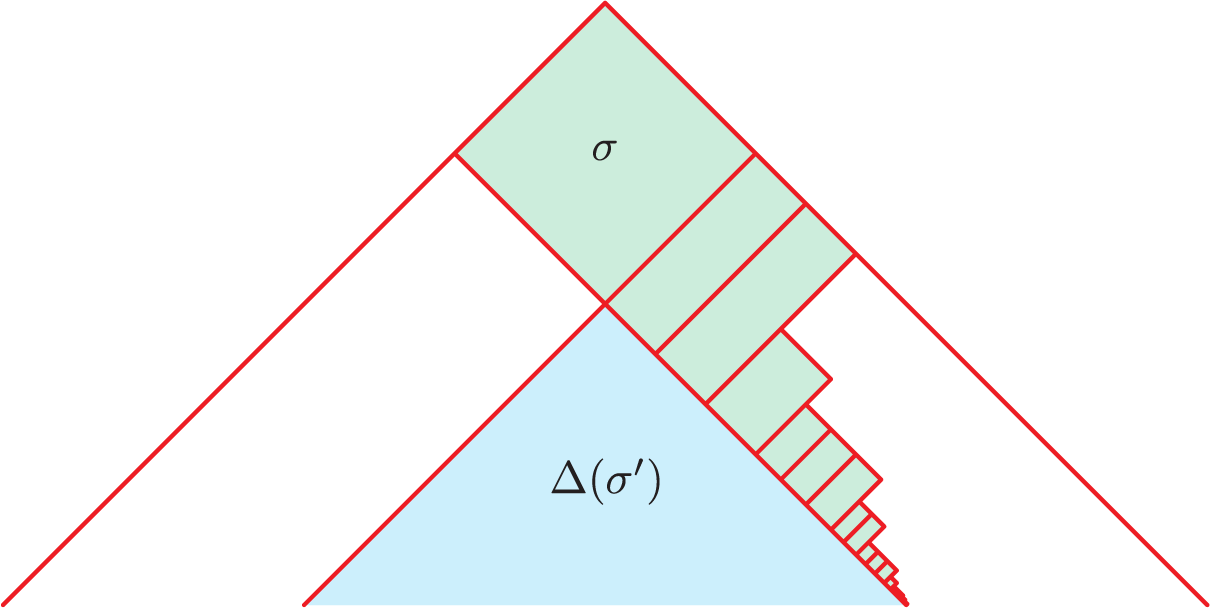
The descending set of a sector
 $\sigma $
, and part of its intersection with
 $\widetilde \Gamma $
(in colour online).

Local pictures of vertices in Q and incident
 $\widetilde \Gamma $
-edges (red) and
 $\widetilde \Phi $
-edges (green) in the proof of Lemma 3.1. All edges are directed upward. Note that there are always incoming
 $\widetilde \Phi $
-edges (the number may vary) and a unique outgoing
 $\widetilde \Phi $
-edge (in colour online).

Clearly,
 $\Delta (\sigma ) \subset Q$
, since no descending paths starting at
 $\sigma $
can cross the branch lines through v.
For the reverse containment, let
 $S_n$
denote the set of
 $\widetilde B^s$
-sectors reachable from
 $\sigma $
by a descending path traversing at most n sectors. Then
 $\sigma = S_1\subset S_2\subset S_3\subset \cdots $
is an exhaustion of
 $\Delta (\sigma )$
.
Claim 3.2. If w is a vertex in the boundary of
 $S_n$
, then either w is in the interior of
 $S_{n+1}$
or it lies on one of the two branch lines through v and hence on the boundary of Q.
Proof of claim
The proof is by induction with the case of
 $S_1 = \sigma $
being by inspection (see Figure 6).
Now suppose that w is in the boundary of both
 $S_n$
and
 $S_{n+1}$
. By the inductive hypothesis, we may assume that w is a vertex of a sector
 $\sigma ' \subset S_n \smallsetminus S_{n-1}$
. In particular, w is not the top vertex of
 $\sigma '$
. If w is not joined by a
 $\widetilde \Gamma $
-edge to the top of
 $\sigma '$
, then again it is clear from the picture (Figure 6) that w is in the interior of
 $S_{n+1}$
, which contradicts our assumption.
Otherwise, w is joined by an edge e to the top vertex
 $w'$
of
 $\sigma '$
and we say that w is one of the two side vertices of
 $\sigma '$
. Note that e is in the boundary of
 $S_n$
, since otherwise we would again have that w is in the interior of
 $S_{n+1}$
.
It suffices to show that e is an edge of a branch line through the vertex v. Note that
 $w'$
is a vertex of some sector
 $\sigma "$
in
 $S_{n-1}$
since any descending path from
 $\sigma $
to
 $\sigma '$
passes through one of the two top edges of
 $\sigma '$
. Since w is not in the interior of
 $S_{n+1}$
, we must have that
 $\sigma '$
is attached to
 $\sigma "$
along the edge
 $e'$
, where
 $e'$
is the
 $\widetilde \Gamma $
-edge at the top of
 $\sigma '$
that is not e. By the induction hypothesis, either
 $w'$
is in the interior of
 $S_{n}$
or
 $w'$
is contained in a branch line through v. However, if
 $w'$
is in the interior of
 $S_n$
, then e is also in the interior of
 $S_n$
, which is a contradiction. Hence, we must have that
 $w'$
lies along a branch line though v. Since
 $e'$
is in the interior of
 $S_n$
, this branch line continues along e, establishing that it contains w. This completes the proof of Claim 3.2.
We conclude that
 $\Delta (\sigma )$
is a subcomplex of the quarter plane Q (with its locally finite tessellation by sectors) and that
 $\partial \Delta (\sigma ) = \partial Q$
. It follows easily that
 $Q = \Delta (\sigma )$
as required.
For part (b), again let
 $S_n$
denote the set of
 $\widetilde B^s$
-sectors reachable from
 $\sigma $
by a descending path traversing at most n sectors. If w is a vertex of
 $S_n$
, then any
 $\widetilde \Gamma $
-path in
 $\Delta (\sigma )$
remains within
 $S_n$
. Since
 $S_n$
has finitely many vertices and
 $\widetilde \Gamma $
-rays are simple, each
 $\widetilde \Gamma $
-ray starting at w eventually meets
 $\partial \Delta (\sigma )$
. This proves part (b).
Considering a picture makes the first claim of part (c) clear; see Figure 7.
The same argument as that for part (b) shows that the
 $\widetilde \Phi $
-ray starting from any point in
 $\Delta (\sigma )$
must meet
 $\partial \Delta (\sigma )$
. This completes the proof of Lemma 3.1.
Next we describe and analyze a canonical set associated to a
 $\widetilde \Gamma $
-ray. For a vertex v or directed edge e of
 $\widetilde \Gamma $
, we set
 $\sigma (v)$
and
 $\sigma (e)$
to be the sector into which the maw vector field points at v or along the interior of e, respectively. So if v is the terminal vertex of the edge e and
 $\sigma $
is the unique sector of
 $\widetilde B^s$
whose top vertex is v, then
 $\sigma (v)= \sigma (e) = \sigma $
.
Lemma 3.3. Suppose there exists a directed path in
 $\widetilde \Gamma $
from u to v. Then
 $\Delta (\sigma (u)) \subset \Delta (\sigma (v))$
.
Proof. The lemma follows by induction on the length of the path from u to v. The inductive step is immediate from the observation that if e is an edge of
 $\widetilde \Gamma $
with initial vertex u and terminal vertex v, then there is a descending path from
 $\sigma (v) = \sigma (e)$
to
 $\sigma (u)$
. Hence,
 $\Delta (\sigma (u)) \subset \Delta (\sigma (v))$
.
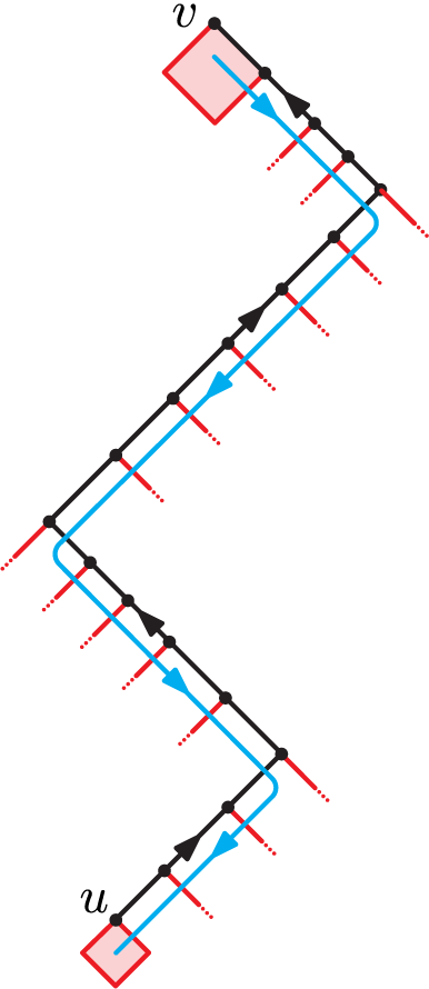
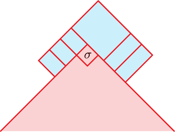
Remark 3.4. The descending path that the proof of Lemma 3.3 produces can be obtained by pushing the dual path from u to v slightly in the direction of the maw vector field and reversing orientation, as shown in Figure 8.
If there is a path in
 $\widetilde \Gamma $
from u to v (shown in black), then there is a descending path in
 $\widetilde B^s$
from
 $\sigma (v)$
to
 $\sigma (u)$
(shown in blue) (in colour online).

Let
 $\gamma $
be a
 $\widetilde \Gamma $
-ray, and set
 $$ \begin{align*} D(\gamma)=\bigcup_{v \in\gamma}\Delta(\sigma(v)), \end{align*} $$
where the unions are taken over all
 $\widetilde \Gamma $
-vertices v traversed by
 $\gamma $
. By Lemma 3.3, it follows that
 $D(\gamma )$
is a nested union of quarter planes. If
 $\gamma $
is not eventually a branch ray of
 $\widetilde \Gamma $
, then
 $D(\gamma )$
is evidently diffeomorphic to
 $\mathbb {R}^2$
and we say that
 $D(\gamma )$
is the dynamic plane associated to
 $\gamma $
. By construction,
 $D(\gamma )$
is properly embedded in
 $\widetilde B^s$
. If
 $\gamma $
is eventually a branch ray, then
 $D(\gamma )$
is diffeomorphic to a half plane and we say that
 $D(\gamma )$
is the dynamic half plane associated to
 $\gamma $
.
We remark that any dynamic plane D is tessellated by sectors of
 $\widetilde B^s$
and hence it makes sense to speak of
 $\widetilde \Gamma $
-paths or
 $\widetilde \Phi $
-paths in D. Moreover,
 $\widetilde \Gamma \cup \widetilde \Phi $
determine a triangulation of D.
Remark 3.5. Since
 $\sigma (v) = \sigma (e)$
for an edge e of
 $\widetilde \Gamma $
with terminal vertex v, we also have
 $$ \begin{align*} D(\gamma) = \bigcup_{e \in\gamma}\Delta(\sigma(e)), \end{align*} $$
where the union is over edges traversed by
 $\gamma $
.
Proposition 3.6. (Basics of dynamic planes)
Let D be a dynamic plane.
-
(a) For any edge e of D,
$\Delta (\sigma (e)) \subset D$
. -
(b) If
$\gamma $
is any
$\widetilde \Gamma $
-ray contained in D that is not eventually a branch ray, then
$D = D(\gamma )$
. -
(c) The stabilizer of D is either infinite cyclic or trivial.



Proof. First note that since D is a plane properly embedded in
 $\widetilde B^s$
, if D contains e, then D contains
 $\sigma (e)$
. This follows since
 $\sigma (e)$
is the sector on the
 $1$
-sheeted side of e. Next, suppose that
 $D = D(\psi )$
for some
 $\widetilde \Gamma $
-ray
 $\psi $
that is not eventually a branch ray. If
 $\sigma \subset D(\psi )$
, then directly from the definitions we have that
 $\Delta (\sigma ) \subset D(\psi )$
. Taken together, these two facts prove part (a).
For part (b), note that part (a) implies that
 $D(\gamma ) \subset D$
(see Remark 3.5). Since these are each planes properly embedded in
 $\widetilde B^s$
, equality also holds.
For part (c), we appeal to the discussion preceding the proof of Lemma 3.1. Since the dynamic plane D is carried by
 $B^s$
, it determines a unique leaf
 $\widetilde \ell $
of
 $\widetilde {\mathcal L}^s$
such that
 $D = \operatorname {\mathrm {coll}} (\widetilde \ell )$
. Hence, the stabilizer of D is equal to the stabilizer of
 $\widetilde \ell $
and the claim follows from the fact that the image of
 $\widetilde \ell $
in M is either a plane, annulus, or Möbius band.
Recall that if
 $\gamma $
is a
 $\widetilde \Gamma $
-path or ray contained in D which makes only AB turns, we say
 $\gamma $
is an AB path or AB ray. Then each two consecutive
 $\widetilde \Gamma $
-edges of
 $\gamma $
determine a triangle in the triangulation of D by edges of
 $\widetilde \Phi $
and
 $\widetilde \Gamma $
, and the third edge of this triangle is a
 $\widetilde \Phi $
-edge. The union of all these triangles is a subset S of D diffeomorphic to
 $[0,1]\times [0,1]$
or
 $[0,1]\times [0,\infty )$
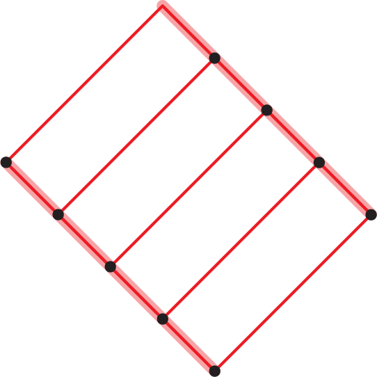
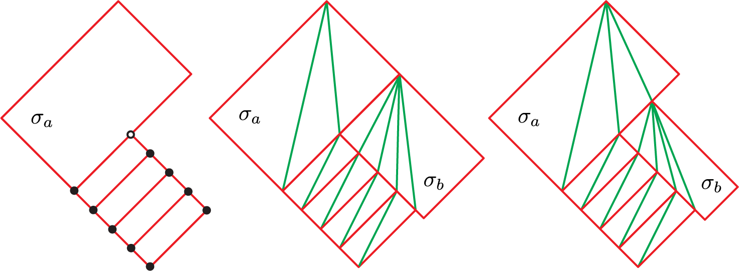
called an AB strip or infinite AB strip, respectively. See Figure 9.
An AB strip (left) and an infinite AB strip (right), with
 $\widetilde \Gamma $
-edges in red and
 $\widetilde \Phi $
-edges in green. Edges are directed upward (in colour online).

The following lemma essentially says that
 $\widetilde \Phi $
-rays in a dynamic plane either converge or are separated by AB strips.
Lemma 3.7. (Dynamics of dynamic planes)
Let D be a dynamic plane. If
 $\alpha $
and
 $\beta $
are
 $\widetilde \Phi $
-rays contained in D, then either
 $\alpha $
and
 $\beta $
eventually coincide or both eventually lie on the boundaries of infinite AB strips.
Proof. Suppose that
 $D = D(\gamma )$
, where
 $\gamma $
is a
 $\widetilde \Gamma $
-ray which is not eventually a branch ray, and let
 $p_1,p_2,\ldots $
be the sequence of vertices where
 $\gamma $
makes AB turns. Define
 $\Delta _i=\Delta (\sigma (p_i))$
, so that
 $\Delta _1\subset \Delta _2\subset \Delta _3\subset \cdots $
is the exhaustion of
 $D(\gamma )$
by descending sets. Let a and b be vertices of
 $\alpha $
and
 $\beta $
, respectively. By truncating and reindexing the exhaustion
 $\{\Delta _i\}$
, we can assume that a and b lie in
 $\Delta _1$
. Hence by Lemma 3.1(b), there exist vertices
 $a_1$
of
 $\alpha $
and
 $b_1$
of
 $\beta $
lying on the boundary of
 $\Delta _1$
, and
 $a_1$
and
 $b_1$
are a finite distance apart in the combinatorial metric on
 $\partial \Delta _1$
.
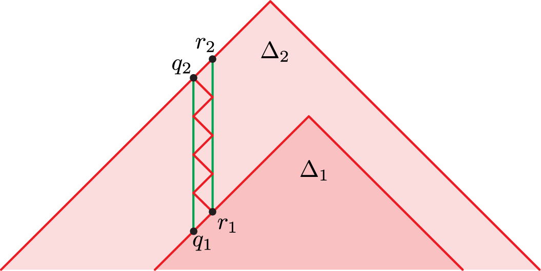
Let
 $q_1,r_1\in \partial \Delta _1$
be vertices that are connected by an edge from
 $q_1$
to
 $r_1$
with
 $\widetilde \Phi $
-rays intersecting
 $\partial \Delta _2$
in
 $q_2$
and
 $r_2$
respectively. We claim that
 $ q_2\ne r_2$
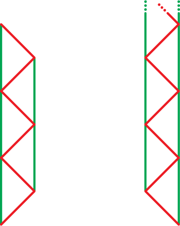
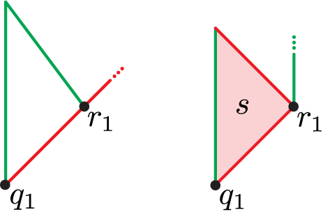
if and only if the corresponding ray segments cobound an AB-strip (see Figure 10). Indeed, if s is the sector in D above the
 $\widetilde \Gamma $
-edge connecting
 $q_1$
and
 $r_1$
, then the
 $\widetilde \Phi $
-rays from
 $q_1$
and
 $r_1$
immediately converge unless
 $r_1$
is a corner vertex of s as in Figure 11. Applying this analysis repeatedly proves the claim. In other words, ‘flowing’ forwards in D weakly contracts distance in
 $\partial \Delta _i$
, with equality if and only if the flow segments are separated by a union of AB strips. This implies that either the rays from
 $a_1$
and
 $b_1$
eventually coincide, or they both eventually meet AB rays.
AB strips are precisely the obstruction to contraction under ‘flowing’ forward in a dynamic plane (in colour online).

The flow rays from
 $q_1$
and
 $r_1$
immediately collide (left) unless
 $r_1$
is a corner vertex of the sector s above
 $q_1$
(right) (in colour online).

We next require a basic lemma about the structure of
 $\widetilde B^s$
. Recall that each
 $\widetilde B^s$
-sector has two sides, a top vertex and bottom vertex, and two corner vertices. Each side of a sector is composed of two branch segments, one which begins at the bottom vertex and terminates at a corner vertex, and one which consists of precisely one
 $\widetilde \Gamma $
-edge which begins at the corner vertex and terminates at the top vertex. Each of these vertices corresponds to a triple point of
 $\widetilde B^s$
, and has a right or left veer as shown in Figure 12. This veer agrees with the veer of the edge atop the unique tetrahedron containing the triple point (compare with Figure 3).
Each triple point in
 $B^s$
comes with a veer (in colour online).

In this language, we have the following lemma, which is a reformulation of [Reference Landry, Minsky and TaylorLMT20, Fact 1]. For an illustration of the behavior described in the lemma, see Figure 13.
Some situations allowed by Lemma 3.8, where x and y denote opposite veers. Note that the veers of top vertices are not governed by the lemma (in colour online).

Lemma 3.8. Let A be a
 $B^s$
-sector. The bottom vertex and two corner vertices have identical veer. All other vertices in
 $\partial A$
, except possibly the top vertex, have the opposite veer.
Recall from above that an infinite AB strip is a subset of a dynamic plane homeomorphic to
 $[0,1]\times [0,\infty )$
, determined by an AB ray. The subsets of an infinite AB strip corresponding to
 $\{0,1\}\times [0,\infty )$
are
 $\widetilde \Phi $
-rays. Similarly, we define a bi-infinite AB strip to be a subset of a dynamic plane homeomorphic to
 $[0,1]\times \mathbb {R}$
determined by an AB line. The boundary components of a bi-infinite AB strip are
 $\widetilde \Phi $
-lines.
Lemma 3.9. Let D be a dynamic plane. The following are equivalent:
-
(i) D contains an infinite AB strip;
-
(ii) D contains a bi-infinite AB strip;
-
(iii) D contains the lift of an AB-cycle.
Proof. For the equivalence of conditions (i) and (ii), note that every vertex in D has a unique backward AB ray (Figure 7), so every infinite AB strip is part of a bi-infinite AB strip. Since every AB line covers an AB-cycle, the other implications are clear.
Recall that each
 $\widetilde \tau $
-edge e has two fans, consisting of the tetrahedra for which e is a
 $0$
-edge lying on a particular side of e. The length of a fan in
 $\widetilde \tau $
is the number of tetrahedra it contains. We can also define fans and their lengths for edges of
 $\tau $
by lifting to
 $\widetilde \tau $
.
We denote the length of the longest fan in
 $\tau $
by
 $\delta _{\tau }$
.
Proposition 3.10. (The AB region)
Suppose that D contains a bi-infinite AB strip. Then:
-
(1) the number of bi-infinite AB strips in D is less than
$\delta _{\tau }$
; and -
(2) the union
$D_{\text {AB}}$
of all bi-infinite AB strips in D is diffeomorphic to
$[0,1]\times \mathbb {R}$
.


The union
 $D_{\text {AB}}$
of all bi-infinite AB strips in D, as in Proposition 3.10, will be called the AB region of D.
Proof. By Lemma 3.7, if D contains n or more infinite AB strips, then there is a subset S of D that is obtained by gluing n infinite AB strips along their
 $[0,\infty )$
boundaries. See Figure 14. By Lemma 3.8, all the vertices in the interior of S have identical veer, so if v is a vertex in the interior of S, then v lives in a tetrahedron whose top and bottom edges have the same veer. In other words, every vertex in the interior of S lies in a non-hinge tetrahedron. Any branch line traversing S therefore must pass through
 $n-1$
consecutive non-hinge tetrahedra.
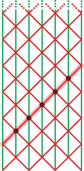
A picture of the set S in the proof of Proposition 3.10. The
 $\widetilde \Phi $
-edges are shown in green. By Lemma 3.8, each vertex in the interior of S has the same veer. The highlighted branching segment passes through five consecutive non-hinge tetrahedra, corresponding to the vertices colored black (in colour online).

We now need a combinatorial fact about veering triangulations.
Claim 3.11. If a branch line
 $\gamma $
passes through consecutive non-hinge tetrahedra
 $T_1,\ldots , T_k$
, then the
 $T_i$
all lie in the fan of a single edge e.
Proof. Suppose without loss of generality that the top and bottom edges of
 $T_1$
are right veering. The branching line
 $\gamma $
passes through two faces of
 $T_1$
which meet along a left veering edge E of
 $T_1$
by [Reference Landry, Minsky and TaylorLMT20, Lemma 4.5]. We call these faces
 $f_1$
and
 $f_2$
, where
 $f_1$
is a bottom face for
 $T_1$
and
 $f_2$
is a top face for
 $T_1$
. If
 $f_3$
is the next face passed through by
 $\gamma $
, [Reference Landry, Minsky and TaylorLMT20, Lemma 4.5] again implies that
 $f_2$
and
 $f_3$
meet along a left veering edge of
 $T_2$
. Since e is the only left veering edge of
 $f_2$
, we conclude that
 $f_1, f_2, f_3$
are all incident to e, and that
 $T_1$
and
 $T_2$
lie in the same fan of e. Continuing in this way shows that each
 $T_i$
is in this fan. This completes the proof of Claim 3.11.
Returning to the proof of Proposition 3.10: since any fan of length
 $>1$
containing non-hinge tetrahedra contains two distinct hinge tetrahedra and any non-hinge tetrahedron is part of such a fan (see e.g. [Reference Futer and GuéritaudFG13, Observation 2.6]), Claim 3.11 implies that there exists a fan of
 $\tau $
with size at least
 $n+1$
. Hence, the number of bi-infinite AB strips in D is less than the length
 $\delta _{\tau }$
of the longest fan in
 $\tau $
, proving item (i).
Now suppose that D contains exactly n bi-infinite AB strips, and let g be the generator of the stabilizer of D. Let s and
 $s'$
be two adjacent such strips in the sense that there are no strips between them. It is clear that g permutes the set of bi-infinite AB strips in D; let
 $g'$
be a power of g preserving s and
 $s'$
. By Lemma 3.7, two of the boundary
 $\widetilde \Phi $
-lines of s and
 $s'$
eventually coincide. Since
 $s\cup s'$
is g-invariant, these boundary
 $\widetilde \Phi $
-lines must be equal. Applying this argument
 $n-1$
times establishes item (ii).
Remark 3.12. If a dynamic plane D contains at least two bi-infinite AB strips, then it corresponds to a region of the triangulation that Agol and Tsang call a wall in their work-in-progress [Reference Agol and TsangAT21]. A key property, which they point out, is that these regions prevent
 $\Phi $
from being strongly connected. From our perspective, this can be seen by noting that when there are at least two AB strips in D, there will be at least one component of
 $\widetilde \Phi \cap D$
which is a properly embedded line. Such a line descends to a
 $\Phi $
-cycle in M that is a circular source in the sense that it has no other incoming
 $\Phi $
-edges.
We say that two
 $\widetilde \Phi $
-rays are asymptotic if they eventually agree. It is clear that asymptoticity is an equivalence relation on
 $\widetilde \Phi $
-rays. We define the width of a dynamic plane D, denoted
 $w(D)$
, to be the number of asymptotic classes of
 $\Phi $
-rays contained in D. Lemma 3.7 and Proposition 3.10 imply the following.
Corollary 3.13. (Width of dynamic planes)
Let D be a dynamic plane. The width
 $w(D)$
of D satisfies
 $$ \begin{align*} w(D)&=1+(\# \text{ of bi-infinite AB strips in } D)\\ &\le \delta_{\tau}. \end{align*} $$
The following lemma characterizes when the quotient of a dynamic plane is an annulus in terms of the veering combinatorics.
Lemma 3.14. Let
 $\gamma $
be a
 $\Gamma $
-cycle which is not a branch curve. Let
 $\widetilde \gamma $
be a lift to
 $\widetilde M$
, and let
 $g \in \pi _1(M)$
generate the stabilizer of
 $\widetilde \gamma $
. Then
 $L = D(\widetilde \gamma )/ \langle g \rangle $
is an annulus if and only if
 $\gamma $
has an even number of AB-turns.
Proof. In [Reference Landry, Minsky and TaylorLMT20, Lemma 5.6], it is shown that
 $\gamma $
has an even number of AB-turns if and only if the pullback of the tangent bundle over
 $B^s$
is orientable. However, the immersion
 $\gamma \to B^s$
factors through the immersion
 $L \to B^s$
, and so
 $\gamma $
has an even number of AB-turns if and only if L is orientable. From this, the lemma easily follows.
The following proposition is a key technical result of this section.
Proposition 3.15. (
$\Phi $
sees most
$\Gamma $
-cycles)


Let
 $\gamma $
be a
 $\Gamma $
-cycle. Then
 $\gamma $
is either homotopic to a
 $\Phi $
-cycle or to an AB-cycle of odd length.
In particular, the dual cycles that are not homotopic to flow cycles form a finite set of homotopy classes, up to positive multiples.
Proof. In the proof of [Reference Landry, Minsky and TaylorLMT20, Proposition 5.7], it is explained that every branch curve is homotopic to a
 $\Phi $
-cycle. Hence, we can assume that
 $\gamma $
is not a branch curve. It follows that any lift of
 $\gamma $
to
 $\widetilde M$
determines a dynamic plane.
Let
 $\widetilde \gamma $
be a lift of
 $\gamma $
to
 $\widetilde M$
and let
 $D = D(\widetilde \gamma )$
. Let g be the deck transformation of
 $\widetilde M$
that generates the stabilizer of
 $\widetilde \gamma $
and translates
 $\widetilde \gamma $
in the positive direction. Then
 $g D = D$
, so
 $\gamma $
lifts to the core of
 $L = D / \langle g \rangle $
, which is either an open annulus or open Möbius band. We abuse notation slightly by referring to the images of
 $\widetilde \Phi $
and
 $\widetilde \Gamma $
in L as
 $\Phi $
and
 $\Gamma $
.
If the width
 $w(D)$
is equal to
 $1$
and
 $\widetilde \rho $
is any
 $\widetilde \Phi $
-ray contained in D, then
 $\widetilde \rho $
and
 $g\cdot \widetilde \rho $
eventually coincide. This follows from Lemma 3.7 and the fact that if
 $w(D) = 1$
, then D has no infinite
 $AB$
strips (Lemma 3.9). It follows that
 $\widetilde \rho $
is eventually g-periodic, and projects to a
 $\Phi $
-cycle
 $\rho $
homotopic to the core of L. Hence,
 $\gamma $
is homotopic to
 $\rho $
, proving the claim in this case.
If
 $w(D)>1$
, then D has a non-empty AB region
 $D_{\text {AB}}$
. Let
 $L_{\text {AB}}$
denote the image of this AB region in L. Note that since
 $D_{\text {AB}}$
is g-invariant,
 $L_{\text {AB}}$
is an annulus or Möbius band if and only if L is an annulus or Möbius band, respectively. We finish the proof by considering three cases.
-
• If
$L_{\text {AB}}$
is an annulus, then there are
$w(D)$
parallel
$\Phi $
-cycles in
$L_{\text {AB}}$
homotopic to the core of L, so
$\gamma $
is homotopic to a
$\Phi $
-cycle. -
• If
$L_{\text {AB}}$
is a Möbius band and
$w(D)$
is odd, then there is a single
$\widetilde \Phi $
-line bisecting the AB region of D which projects to a
$\Phi $
-cycle in L and which is homotopic to the core of L, so
$\gamma $
is homotopic to a
$\Phi $
-cycle. -
• Finally, if
$L_{\text {AB}}$
is a Möbius band and
$w(D)$
is even, then there is a bi-infinite AB strip bisecting the AB region of D whose core AB cycle projects to a
$\Gamma $
-cycle in L homotopic to the core of L. By Lemma 3.14, this AB cycle has odd length, so
$\gamma $
is homotopic to an odd AB cycle.


3.2 Homotopy in dynamic planes
We conclude this section with an additional fact, Lemma 3.17, about dynamic planes that will be necessary in §6. In its proof, we will use the following lemma.
Lemma 3.16. If
 $\gamma _1$
and
 $\gamma _2$
are distinct directed paths in
 $\widetilde \Gamma $
with common endpoints, then each
 $\gamma _i$
contains an anti-branching turn.
Proof. Let u and v be the initial and terminal vertices of
 $\gamma _1$
and
 $\gamma _2$
, respectively. By shortening the paths, we may assume u and v are the only common vertices of
 $\gamma _1$
and
 $\gamma _2$
. Let D be a dynamic plane containing
 $\gamma _1$
and
 $\gamma _2$
, and let A be the disk component of
 $D\setminus (\gamma _1\cup \gamma _2)$
. Considering the local structure of the branch locus of
 $\widetilde B^s$
, we see that the maw vector field must point into A along the terminal edges of
 $\gamma _1$
and
 $\gamma _2$
, and out of A along the initial edges of
 $\gamma _1$
and
 $\gamma _2$
. Since the maw vector field switches between pointing inward and outward at exactly the anti-branching turns, we conclude that each
 $\gamma _i$
contains an odd, and in particular non-zero, number of anti-branching turns.
As a consequence, a path in
 $\widetilde \Gamma $
that deviates from a branch line can never return to that branch line.
Let D be a dynamic plane stabilized by some
 $g \in \pi _1(M)$
. As before, let L denote the quotient
 $D/ \langle g \rangle $
. Consider a
 $\Gamma $
-cycle
 $\gamma $
contained in L. If there is a sector
 $\sigma $
of L such that
 $\gamma $
runs along a side of
 $\sigma $
from its bottom vertex to its top vertex, then we may perform a homotopy of
 $\gamma $
, supported on
 $\sigma $
, that pushes
 $\gamma $
from one side of
 $\sigma $
to the other side of
 $\sigma $
. We refer to this homotopy as sweeping across the sector
 $\sigma $
. See Figure 27, where it is shown that sweeping across a sector is a homotopy through curves that are transverse to
 $\tau ^{(2)}$
.
Lemma 3.17. Let D be a dynamic plane stabilized by
 $g \in \pi _1(M) \smallsetminus \{1\}$
. Let
 $\widetilde \gamma _1$
and
 $\widetilde \gamma _2$
be g-invariant
 $\widetilde \Gamma $
-lines contained in D and assume that neither is a branch line. Then
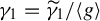 $\gamma _1 = \widetilde \gamma _1 /\langle g \rangle $
is homotopic to
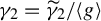 $\gamma _2 = \widetilde \gamma _2 /\langle g \rangle $
in
 $L = D/ \langle g \rangle $
by a homotopy that sweeps across sectors.
Proof. The embedded dual cycles
 $\gamma _1, \gamma _2$
in L either intersect or not. If they intersect and are distinct, there is at least one connected component U of
 $L-(\gamma _1\cup \gamma _2)$
with closure homeomorphic to a disk. Let
 $p_1$
and
 $p_2$
be the two segments of
 $\gamma _1$
and
 $\gamma _2$
which cobound U. By Lemma 3.16, each of
 $p_1$
and
 $p_2$
contains an anti-branching turn.
Let
 $(d_1, d_2)$
be the first anti-branching turn of, say,
 $p_1$
. Since U is tiled by sectors, it must be the case that
 $p_1$
traverses an entire side of
 $\sigma (d_2)$
. When we sweep
 $\gamma _1$
across
 $\sigma (d_2)$
, we shrink the region U by
 $1$
sector. It follows that after sweeping across finitely many sectors, we can homotope
 $\gamma _1$
to
 $\gamma _2$
.
Next, suppose that
 $\gamma _1$
and
 $\gamma _2$
do not intersect. Note that this is not possible if L is a Möbius band and so we may assume that L is an annulus. Then there is a unique component of
 $L-(\gamma _1\cup \gamma _2)$
with compact closure, which we also call U; note that U is an annulus with boundary components
 $\gamma _1$
and
 $\gamma _2$
.
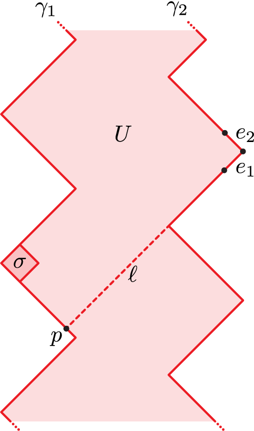
Let
 $(e_1,e_2)$
be an AB turn of
 $\gamma _2$
such that
 $\sigma (e_2)\subset U$
, that is, the maw vector field points into U along
 $e_2$
. Such a turn exists since
 $\gamma _2$
has a non-zero even number of anti-branching turns by Lemma 3.14. Let
 $\ell $
be the branch line through
 $e_1$
. We claim that
 $\ell $
intersects
 $\gamma _1$
in addition to
 $\gamma _2$
. To see this, first note that the negative subray of
 $\ell $
from
 $e_2$
(which is entirely contained in L) is not entirely contained in U, since U is tiled by finitely many sectors. Further, this negative subray cannot return to
 $\gamma _2$
by Lemma 3.16.
Therefore, the negative subray of
 $\ell $
from
 $e_1$
must intersect
 $\gamma _1$
, as in Figure 15. Let p be the first vertex of intersection between this negative ray and
 $\gamma _1$
. Let
 $(f_1,f_2)$
be the first anti-branching turn of
 $\gamma _1$
after p, and let
 $\sigma =\sigma (f_2)$
. If
 $\ell '$
is the branching line through
 $f_1$
, then the bottom of
 $\sigma $
can lie no lower on
 $\ell '$
than p. Hence,
 $\gamma _1$
traverses the entire left side of
 $\sigma $
and can be homotoped across
 $\sigma $
, shrinking the size of U by one sector. After applying this argument finitely many times, we are finished.
Notation from the proof of Lemma 3.17 (in colour online).

4 Pseudo-Anosov flows and veering triangulations
In this and subsequent sections, we will be primarily interested in a pseudo-Anosov flow
 $\varphi $
without perfect fits on a closed
 $3$
-manifold
 $\overline M$
, as well as the manifold M obtained by removing from
 $\overline M$
the singular orbits of
 $\varphi $
. In this setting, the construction of Agol–Guéritaud (Theorem 4.7) produces a veering triangulation
 $\tau $
on a manifold N that is homeomorphic to M. Here we review some necessary background and terminology, with the essential properties of
 $\varphi $
summarized in Lemma 4.2. In §5, we will show
 $\tau $
can be realized as a triangulation of M such that flow lines of
 $\varphi $
are positively transverse to
 $\tau ^{(2)}$
.
First, let
 $\varphi $
be a pseudo-Anosov flow on the closed
 $3$
-manifold
 $\overline M$
. We refer the reader to [Reference Fenley and MosherFM01, §4] for the precise definition, and informally summarize the features of
 $\varphi $
as follows:
-
•
$\varphi $
has finitely many (and at least one) singular periodic orbits where the return map on a transverse disk is locally modeled on a pseudo-Anosov surface homeomorphism near an
$(n\ge 3)$
-pronged singularity; -
• the orbits of the flow are
$C^1$
and
$\varphi $
is smooth away from its singular orbits; -
• there is a pair of mutually transverse two-dimensional singular foliations, called the stable and unstable foliations, whose leaves intersect in exactly the orbits of
$\varphi $
, such that orbits in a leaf of the stable foliations are exponentially contracted under
$\varphi $
and the orbits in a leaf of the unstable foliation are exponentially expanded.


A non-singular closed orbit
 $\gamma $
of
 $\varphi $
is orientable or untwisted if the stable leaf containing it is homeomorphic in the path topology to an annulus. Otherwise, the orbit is called non-orientable or twisted and the stable leaf is a Möbius band.
Let
 $\mathcal Q$
denote the flow space of
 $\varphi $
for
 $\overline M$
, that is, the space obtained by lifting to the universal cover
 $\widetilde { \overline M}$
and collapsing flow lines of the lifted flow. According to Fenley–Mosher [Reference Fenley and MosherFM01, Proposition 4.1],
 $\mathcal Q$
is homeomorphic to the plane and the lifts of the stable/unstable foliations of
 $\varphi $
project to a pair of transverse singular foliations
 $\mathcal F^{s/u}$
on
 $\mathcal Q$
. The points of
 $\mathcal Q$
that are the images of (lifted) singular orbits of
 $\varphi $
are called the singularities of
 $\mathcal Q$
. Note that there is a natural action
 $\pi _1(\overline M) \curvearrowright \mathcal Q$
by orientation-preserving homeomorphisms, where the orientation on
 $\mathcal Q$
is induced by the fixed orientation on
 $\overline M$
and the orientation on flow lines.
Similarly, we let
 $\mathring {\mathcal P}$
denote the flow space of M, defined by the same procedure, which can also be obtained by taking the universal cover of
 $\mathcal Q$
minus its singularities. From this, we see that
 $\mathring {\mathcal P}$
is also homeomorphic to the plane. Moreover, this perspective allows us to define the completed flow space
 $\mathcal P$
of M as the corresponding branched cover
 $\mathcal P \to \mathcal Q$
infinitely branched over the singularities of
 $\mathcal Q$
. We also call the branch points of this map the singularities of
 $\mathcal P$
. Since singularities of
 $\mathcal Q$
are discrete, so are the singularities of
 $\mathcal P$
. Throughout, we extend terminology for
 $\mathcal Q$
to
 $\mathcal P$
by lifting. For example, we continue to denote the lifted singular foliations on
 $\mathcal P$
by
 $\mathcal F^{s/u}$
. There is also an orientation-preserving action
 $\pi _1(M) \curvearrowright \mathcal P$
by homeomorphisms that makes the branched cover
 $\mathcal P \to \mathcal Q$
equivariant with respect to the homomorphism
 $\pi _1(M) \to \pi _1(\overline M)$
. The projections to the flow space
 $\widetilde M \to \mathring{\mathcal P}$
and
 $\widetilde {\overline M} \to \mathcal Q$
are oriented line bundles over the plane.
A rectangle R in the flow space
 $\mathcal Q$
or
 $\mathcal P$
is a topological closed disk with no singularities in its interior with boundary consisting of four segments of leaves of
 $\mathcal {F}^s$
and
 $\mathcal {F}^u$
. The boundary of R necessarily consists of two stable leaf segments, which we call the vertical boundary of R and denote
 $\partial _v R$
, and two unstable leaf segments, which we call the horizontal boundary and denote
 $\partial _h R$
. (Note that by convention, we draw
 $\mathcal F^{\kern1.3pt s}$
vertically and
 $\mathcal F^u$
horizontally.) A maximal rectangle is a rectangle that contains a singularity in the interior of each of its sides, and so it is maximal with respect to inclusion.
As an informal definition, we say that a leaf
 $\unicode{x3bb} ^u$
of
 $\mathcal F^u$
and a leaf
 $\unicode{x3bb} ^s$
of
 $\mathcal F^u$
form a perfect fit if they are disjoint but ‘meet at infinity.’ We say that
 $\varphi $
has no perfect fits if its flow space
 $\mathcal Q$
has no perfect fits. We omit the precise definition of a perfect fit (see [Reference FenleyFen12, Definition 2.2]) because, given the fact that singular leaves are dense in
 $\mathcal Q$
(see Lemma 4.2), no perfect fits is equivalent to the condition that every sequence of nested rectangles is contained in a maximal rectangle. The reader can take this as the definition of no perfect fits. It is also proven by Fenley [Reference FenleyFen99a, Theorem 4.8] that when
 $\varphi $
has no perfect fits, each
 $g\in \pi _1(\overline M)$
fixes at most one point of
 $\mathcal Q$
(again see Lemma 4.2). Existence of maximal rectangles and uniqueness of fixed points are the essential properties of
 $\varphi $
that we will use throughout this paper.
Convention 4.1. (No perfect fits)
Henceforth, we will assume that the pseudo-Anosov flow
 $\varphi $
has no perfect fits.
Continuing with terminology, we define an edge rectangle Q to be a rectangle in either
 $\mathcal Q$
or
 $\mathcal P$
with singularities at two of its (necessarily opposite) corners. (These were called spanning rectangles in [Reference Minsky and TaylorMT17]). Each edge rectangle Q has a veer defined as follows: if the singularities of Q are at its SW and NE corners, then Q is right veering. Otherwise, Q is left veering. Here, the position of the singular vertices is determined by an orientation-preserving embedding of Q into
 $\mathbb {R}^2$
for which the restricted foliation
 $\mathcal F^{\kern1.3pt s} \cap Q$
maps to vertical lines and
 $\mathcal F^u \cap Q$
maps to horizontal lines. The veer of Q is well defined and an invariant of the
 $\pi _1$
-actions on
 $\mathcal Q$
and
 $\mathcal P$
since these actions are orientation preserving. A face rectangle is a rectangle with a singularity at one of its corners and singularities in the interiors in each of its sides not containing the singular corner. Note that each face rectangle contains exactly three edge rectangles and is contained in exactly two maximal rectangles. Moreover, each maximal rectangle contains the face and edge rectangles determined by the pairs and triples of its singularities. See Figure 16.
From left to right we see an edge rectangle, a face rectangle, and a maximal rectangle.

We next define a partial order on rectangles in
 $\mathcal Q$
or
 $\mathcal P$
. We call rectangles
 $R_1$
and
 $R_2$
ordered if their interiors intersect but do not contain any of each other’s corners. Assuming
 $R_1$
and
 $R_2$
are ordered, if the interior of
 $R_2$
meets
 $\partial _h R_1$
, then we say that
 $R_2$
is taller than
 $R_1$
. If the interior of
 $R_1$
meets
 $\partial _v R_2$
, then
 $R_1$
is wider than
 $R_2$
. Finally, for ordered rectangles, we say that
 $R_2$
lies above
 $R_1$
if
 $R_1$
is not taller than
 $R_2$
, and
 $R_1$
lies below
 $R_2$
if
 $R_2$
is not wider than
 $R_1$
. Put differently,
 $R_2$
lies above
 $R_1$
if they are ordered and
 $R_2 \cap \partial R_1$
contains a segment in each component of the horizontal boundary of
 $R_1$
. We say that
 $R_2$
lies strictly above
 $R_1$
if
 $R_2$
is taller than
 $R_1$
and
 $R_1$
is wider than
 $R_2$
.
We note that if
 $R_1$
and
 $R_2$
are distinct maximal rectangles, then
 $R_2$
lies above
 $R_1$
if and only if
 $R_2$
is taller than
 $R_1$
if and only if
 $R_1$
is wider than
 $R_2$
. See Figure 17.
Some ways
 $R_2$
can lie above
 $R_1$
.

Properties of the flow
 $\varphi $
translate to properties of the actions
 $\pi _1(\overline M) \curvearrowright \mathcal Q$
and
 $\pi _1(M) \curvearrowright \mathcal P$
. We record these in the following lemma that summarizes results from several papers of Fenley–Mosher, Fenley, and Mosher.
Lemma 4.2. (Properties of the flow space)
With
 $\overline M, \varphi , M, \mathcal Q, \mathcal P$
as above, the following hold.
-
(1) The foliations
$\mathcal F^{s/u}$
are transverse singular foliations of
$\mathcal Q$
with discrete singularities, no saddle connections, and dense singular leaves. -
(2) The stabilizer of any leaf of
$\mathcal F^{s/u}$
is either trivial or infinite cyclic, and each
$g \neq 1$
in a leaf stabilizer fixes exactly one point in that leaf. -
(3) The orbit of any periodic point (that is, point with non-trivial stabilizer) in
$\mathcal Q$
is discrete and periodic points are dense. Moreover, since
$\varphi $
has no perfect fits, each
$g \ne 1$
fixes at most one point in
$\mathcal Q$
. -
(4) Suppose that g fixes a point p of
$\mathcal Q$
, chosen so that g translates the g-periodic flow line projecting to p in its positive direction.-
• If p is non-singular, then for any edge rectangle or maximal rectangle R containing p,
$g(R)$
lies strictly above R. -
• If p is singular and R is a maximal rectangle containing p in its boundary, then either
$g(R)$
and R have disjoint interiors or
$g(R)$
lies strictly above R.
-


Moreover, the corresponding statements for the completed flow space
 $\mathcal P$
also hold.
Proof. The properties listed in item (1) have already been discussed except for the claim that singular leaves are dense in
 $\mathcal Q$
. For this, we first recall that since
 $\overline M$
admits a pseudo-Anosov flow without perfect fits, that is, not conjugate to the suspension of an Anosov diffeomorphism, it is atoroidal [Reference FenleyFen03, Main theorem] (see also the remarks following [Reference FenleyFen12, Theorem D]). Then, since
 $\overline M$
is atoroidal, the flow
 $\varphi $
is transitive by [Reference MosherMos92a, Proposition 2.7]. Finally, [Reference MosherMos92a, Proposition 1.1] and the sentence following it imply that every leaf of the stable and unstable foliations on
 $\overline M$
is dense. Hence, the singular leaves of
 $\mathcal F^{s/u}$
are dense in
 $\mathcal Q$
.
Next, the contracting/expanding dynamics within each leaf of the stable/unstable foliations implies that each non-singular leaf with non-trivial
 $\pi _1$
is either an annulus or Möbius band containing a unique closed orbit (see [Reference MosherMos92a, §1]). From this, item (2) easily follows.
The first statement of item (3) follows from the fact that the orbit of a point in
 $\mathcal Q$
with non-trivial stabilizer corresponds to a closed orbit of
 $\varphi $
in
 $\overline M$
and that the lifts of such an orbit to the universal cover
 $\widetilde {\overline M}$
form a discrete collection of flow lines. The second statement follows from [Reference FenleyFen99a, Theorem 4.8]. There, Fenley shows that if
 $g \neq 1$
fixes distinct points
 $p_1$
and
 $p_2$
, then these points are connected by a so-called chain of lozenges. The existence of a lozenge in
 $\mathcal Q$
, which is essentially a rectangle with two ideal corners, implies that
 $\mathcal Q$
has a perfect fit.
Finally, item (4) follows from considering first return maps to transverse sections of the flow and using the expanding/contracting dynamics.
A more uniform version of item (4) will be useful later. Note first that it is easy to obtain a collection of sections of the bundle
 $\widetilde {\overline M} \to {\mathcal Q}$
over the maximal rectangles, which is equivariant by
 $\pi _1({\overline M})$
, since the group action is free on maximal rectangles (any non-trivial element fixing a maximal rectangle fixes each of its singularities, contradicting Lemma 4.2(3)).
Lemma 4.3. With
 $M, \varphi , {\mathcal Q}$
as above, fix a
 $\pi _1({\overline M})$
-equivariant family of sections
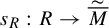 $s_R : R \to \widetilde {\overline M}$
over the maximal rectangles in the flow space. Given
 $\varepsilon>0$
, there is a constant L such that if J is an oriented segment in a non-singular flow line in
 $\widetilde {\overline M}$
of length at least L, so that its forward endpoint lies in the section over a rectangle
 $R_+$
and its backward endpoint lies in the section over a rectangle
 $R_-$
at distance at least
 $\varepsilon $
from the boundary of
 $R_-$
, then
 $R_+$
lies above
 $R_-$
. In fact, both horizontal boundary components of
 $R_-$
pass through the interior of
 $R_+$
and both vertical boundary components of
 $R_+$
pass through the interior of
 $R_-$
.
Proof. Let p be the backward endpoint of J in
 $s_{R_-}(R_-)$
. Let U be the maximal connected set within
 $R_-$
containing p such that the flow from
 $s_{R_-}(R_-)$
to
 $s_{R_+}(R_+)$
is defined on
 $s_{R_-}(U)$
. Then U must be a subrectangle, and the pseudo-Anosov properties of the flow, particularly its expansion on the unstable (horizontal) foliation, implies that the width of
 $s_{R_-}(U)$
is bounded exponentially in
 $-L$
. Thus, for L large enough (depending on
 $\varepsilon $
), the width is small enough that both vertical (stable) sides of
 $\partial U$
are in the interior of
 $R_-$
. Each horizontal side of
 $\partial U$
must therefore lie in the boundary of
 $R_-$
, because otherwise it would be an entire horizontal side of
 $R_+$
, which would imply the interior of
 $R_-$
contains a singular point.
We conclude that
 $R_+$
must cross
 $R_-$
from top to bottom, which proves the claim.
We next observe a few basic consequences. The first essentially says that an infinite sequence of maximal rectangles which is increasing with respect to our partial order ‘lies above’ limits to a leaf of the vertical foliation
 $\mathcal F^{\kern1.3pt s}$
.
Fact 4.4. (Limits of rectangles)
Suppose that
 $(R_i)_{i \in \mathbb {Z}}$
is a sequence of distinct maximal rectangles such that
 $R_{i+1}$
lies above
 $R_i$
for each i.
Then
 $\bigcap _{i \ge 0} R_i$
is a segment of the vertical foliation
 $\mathcal F^{\kern1.3pt s}$
in
 $R_0$
joining the components of
 $\partial _h R_0$
, and
 $\bigcap _{i \le 0} R_i$
is a segment of the horizontal foliation
 $\mathcal F^u$
in
 $R_0$
joining the components of
 $\partial _v R_0$
.
Proof. Note that if
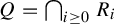 $Q = \bigcap _{i \ge 0} R_i$
is a rectangle with non-empty interior, then we could extend it vertically along leaves of
 $\mathcal F^{\kern1.3pt s}$
to a rectangle
 $Q'$
with singularities in its horizontal boundary. This follows from the density of singular leaves in Lemma 4.2. However, then each
 $R_i$
necessarily lies below
 $Q'$
and so the singularities in the boundary of the
 $R_i$
would have to accumulate in
 $\mathcal Q$
. This contradicts the discreteness of singularities, again as in Lemma 4.2.
The next lemma will be used to show that the veering triangulation discussed in the next section has finitely many simplices.
Lemma 4.5. There are finitely many maximal, face, and edge rectangles in
 $\mathcal Q$
(or
 $\mathcal P$
) up to the
 $\pi _1$
-action.
Before giving the proof, we make a few more observations. Let
 $s\in \mathcal {P}$
be a singularity. There are countably many singular leaves terminating at s; let
 $\ell _1$
and
 $\ell _2$
be two such singular leaves. There is a unique component C of
 $\mathcal {P}-(\ell _1\cup \ell _2)$
whose frontier completely contains
 $\ell _1\cup \ell _2$
. If C contains no singular leaves terminating at s (that is,
 $\ell _1$
and
 $\ell _2$
are ‘neighbors’ at s), then the union
 $\Omega $
of C with
 $\ell _1$
and
 $\ell _2$
is called an orthant. The point s is called the corner singularity of
 $\Omega $
. Note that if
 $\ell _1$
and
 $\ell _2$
bound an orthant, then one is stable and the other is unstable.
Following Guéritaud, we say that a set S of edge rectangles is a staircase if there is an orthant
 $\Omega \subset \mathcal {P}$
with corner singularity
 $s\in \mathcal {P}$
such that S consists of exactly the edge rectangles contained in
 $\Omega $
with one corner at s. See Figure 18. Each orthant determines a unique staircase. Note that all the edge rectangles in a single staircase have common veer. The staircase S has cyclic stabilizer
 $\langle g\rangle \le \pi _1(M)$
, coinciding with the stabilizer of
 $\Omega $
, and our convention will be to choose the generator g so that
 $g Q$
lies above Q for all edge rectangles Q in S. Note, again by discreteness of singularities, there are only finitely many edge rectangles in S that lie above Q and below
 $gQ$
. This allows us to choose an indexing
 $\ldots ,Q_{-1},Q_0,Q_1,\ldots $
of the elements of S so that
 $Q_i$
lies above
 $Q_j$
if and only if
 $i\ge j$
.
Part of a staircase with corner singularity s (in colour online).

Proof of Lemma 4.5
We show that the
 $\pi _1$
-action is cofinite on the edge rectangles in
 $\mathcal Q$
. This immediately implies the same result for
 $\mathcal P$
and the case of face rectangles and maximal rectangles easily follows.
Since each edge rectangle lies in the staircase associated to each of its singular corners and there are only finitely many orthants up to the
 $\pi _1$
action, it suffices to show that for each staircase S, its cyclic stabilizer
 $\langle g \rangle $
acts cofinitely on the edge rectangles of S. This however is clear using the above ordering
 $\ldots ,Q_{-1},Q_0,Q_1,\ldots $
and the fact that g acts on this sequence by increasing the index. This completes the proof.
Since we are interested in the punctured manifold M obtained by removing singular closed orbits from the closed manifold
 $\overline M$
, we introduce some terminology to help remove the need to make special arguments when dealing with the singular orbits. Each singular orbit of
 $\overline M$
has some number of stable/unstable prong curves which are obtained by intersecting the stable/unstable leaves through the singular orbit with the boundary of a small neighborhood of the orbit. We consider the resulting prong curves as peripheral curves in M.
We will use the unstable prong curves to replace the missing singular orbits in our discussion below. For the flow
 $\varphi $
on M, we denote by
 $\mathcal O_{\varphi }$
the periodic orbits of the flow and by
 $\mathcal O_{\varphi }^+$
the periodic orbits plus all positive multiples of the finitely many unstable prong curves.
Remark 4.6. The blown up flow on the compact model for M
One can also think of prong curves in the following way. In [Reference FriedFri82b, §5], Fried explains in detail how one can replace any orbit of a flow by its sphere of normal directions, and obtain a natural flow on the resulting manifold with boundary. If we apply this blowup operation to the singular orbits of
 $\varphi $
on
 $\overline M$
, we obtain a new flow
 $\varphi ^*$
on a manifold
 $M^*$
with toral boundary. The flow
 $\varphi ^*$
is tangent to
 $\partial M^*$
and, when restricted to the interior of
 $M^*$
, conjugate to
 $\varphi $
on M.
On each torus boundary component of
 $M^*$
,
 $\varphi ^*$
has a finite even number of closed orbits, half of which are attracting and half of which are repelling. The attracting orbits correspond to unstable prong curves and the repelling orbits correspond to stable prong curves. While this is an attractive picture, we will continue to work with the flow
 $\varphi $
on the non-compact manifold M.
4.1 The Agol–Guéritaud construction
Let
 $\varphi $
be a pseudo-Anosov flow on
 $\overline M$
with no perfect fits. Here we briefly describe the Agol–Guéritaud construction of a veering triangulation on a manifold homeomorphic to M. We will not dwell on the details here since in the next section, we establish the stronger fact that the veering triangulation can be realized on M so that it is positively transverse to flow lines.
Associate to each maximal rectangle R in the completed flow space
 $\mathcal P$
a taut ideal tetrahedron
 $t_R$
. We identify the ideal vertices of
 $t_R$
with the singularities of R so that the edge rectangles contained in R correspond to edges of
 $t_R$
and faces rectangles correspond to faces of
 $t_R$
. The two angle
 $\pi $
edges of
 $t_R$
are the ones that correspond to edge rectangles spanning the singularities in
 $\partial _h R$
and
 $\partial _v R$
, respectively. Moreover, the coorientations on the faces of
 $t_R$
are determined by declaring that the two bottom faces of
 $t_R$
are the ones which contain the
 $\pi $
edge spanning the singularities in
 $\partial _v R$
. This convention is indicated in Figure 19 by drawing the edge joining the singularities in
 $\partial _h R$
above the edge joining the singularities in
 $\partial _v R$
.
From a maximal rectangle to an ideal tetrahedron. The coorientation convention is indicated by drawing the tetrahedron in the flow space as shown and coorienting its faces to point out of the page. The ideal edges are curvy so as to emphasize that there is no canonical way to draw them.

If faces
 $f_1$
of
 $t_{R_1}$
and
 $f_2$
of
 $t_{R_2}$
determine the same face rectangle in
 $\mathcal P$
(that is, the rectangles spanned by their vertices are equal), then we glue together the corresponding faces. Since each face rectangle is contained in exactly two maximal rectangles, the resulting space
 $\widetilde N$
is a manifold away from its
 $1$
-skeleton. By examining the ways that an edge rectangle can be extended to a maximal rectangle, one similarly verifies that
 $\widetilde N$
is a manifold. It is also the case that
 $\widetilde N$
is contractible.
Since the action of
 $\pi _1(M)$
on
 $\mathcal P$
preserves maximal, face, and edge rectangles, it induces a simplicial action on
 $\widetilde N$
which is cofinite on simplicies (Lemma 4.5). Because distinct singularity stabilizers have trivial intersection (and
 $\pi _1(M)$
is torsion free), each ideal simplex of
 $\widetilde N$
has a trivial stabilizer and the action
 $\pi _1(M) \curvearrowright \widetilde N$
is discontinuous. Moreover, because the peripheral subgroups of
 $\pi _1(M)$
precisely correspond to the stabilizers of singularities in
 $\mathcal P$
, it follows that each of these subgroups acts peripherally on
 $\widetilde N$
. Hence, by a theorem of Waldhausen [Reference WaldhausenWal68, Corollary 6.5], the manifolds M and
 $N = \widetilde N / \pi _1(M)$
are homeomorphic by a homeomorphism that is the identity on
 $\pi _1(M)$
.
Let
 $\tau $
be the induced ideal triangulation of N. It is now straightforward to see that
 $\tau $
is naturally a veering triangulation. The coorientations on the faces of
 $\tau $
come from the convention discussed above and the taut structure on each tetrahedron comes from lifting to
 $\widetilde N$
and ‘projecting’ the tetrahedron to its corresponding maximal rectangle. Note that we are not claiming that there is a single coherent projection from
 $\widetilde N$
to
 $\mathring {\mathcal P}$
, although we will establish this in the next section. An edge is declared to be right veering if its lift to
 $\widetilde N$
determines an edge rectangle in
 $\mathcal P$
whose singularities are at its SW and NE corners. Otherwise, it is left veering.
We summarize this as follows.
Theorem 4.7. (Agol–Guéritaud)
Suppose that
 $\varphi $
is a pseudo-Anosov flow on
 $\overline M$
without perfect fits. Then the above construction produces a veering triangulation
 $\tau $
on a manifold N that is homeomorphic to
 $M = \overline M \smallsetminus \{\text {singular orbits}\}$
.
If the veering triangulation
 $\tau $
comes from the above construction, we say that
 $\tau $
is associated or dual to the flow
 $\varphi $
.
5 Transversality to the flow
Theorem 4.7 constructs the veering triangulation from the structure of the flow space of a pseudo-Anosov flow, but it does not make any claims about how the triangulation and flow coexist in the same manifold. In this section, we show that one can make the two positively transverse in the following sense.
Theorem 5.1. Let
 $\varphi $
be a pseudo-Anosov flow on
 $\overline M$
without perfect fits. Then the veering triangulation
 $\tau $
can be realized in M so that
 $\tau ^{(2)}$
is a smooth cooriented branched surface which is positively transverse to the flow lines of
 $\varphi $
.
Starting with
 $(N,\tau )$
as constructed in the previous section, we will build a homeomorphism
 $N\to M$
which takes
 $\tau $
to the smooth transverse position of Theorem 5.1. The proof has four main steps, which we will summarize.
5.1 Fibration on
$\widetilde N$

We first produce an equivariant fibration
 $p: \widetilde N \to \mathring {\mathcal P}$
, which is an orientation-preserving embedding on each face of
 $\widetilde \tau ^{(2)}$
. The goal is to complete this diagram with an equivariant homeomorphism:

where
 $q:\widetilde M\to \mathring {\mathcal P}$
is the map to the flow space of the flow.
The key step is Proposition 5.2, which gives an embedding of each edge of
 $\widetilde \tau $
in its associated rectangle in
 $\mathring {\mathcal P}$
, so that the three edges of every face have disjoint interiors. In the suspension-flow case, this is simple because the flow space admits an invariant affine structure in which every rectangle is Euclidean, and we may simply use straight lines in Figure 19 (indeed, this is how the original veering picture is obtained). In the general setting, there is no obvious way to do this—equivariance produces some tricky constraints which are reflected in the argument we give in §5.5. Most of the effort of the proof goes into this step. The map p is then produced in Proposition 5.11.
5.2 Compactification and a fiberwise map
We next build a preliminary map that takes p-fibers in
 $\widetilde N$
to q-fibers in
 $\widetilde M$
. However, to have uniform control of it, we compactify N and M and extend the map. We compactify N to a manifold
 $\overline N$
with toral boundary and construct a map
 $\overline h: \overline N \to \overline M$
that takes p-fibers to flow orbits, and boundary tori to singular orbits. Thus, we obtain the diagram

where
 $\widehat N$
and
 $\widehat M$
are completions of
 $\widetilde N$
and
 $\widetilde M$
obtained by lifting the compactifications.
The restriction of
 $\widehat h$
to each fiber may not be an embedding, but we show in Lemma 5.12 that it is proper and degree
 $1$
to its image fiber.
5.3 Straightening the fibers
An averaging step, convolving with a fiberwise bump function, produces a map which is an embedding on the fibers and hence a global homeomorphism. This is carried out in Proposition 5.14, and gives us a topological version of our main result, Proposition 5.15.
5.4 Smoothing
Finally, we address the issue of making the branched surface smooth, and furthermore making sure that the images of edges in the flow space are smooth and transverse to both foliations. The first of these is explained in Proposition 5.16, and the second in Proposition 5.17.
We next turn to carrying out the details.
5.5 Step 1: drawing diagonals and building a fibration
For any points
 $p,q \in \mathcal P$
lying in a maximal rectangle R, but not in a single leaf of
 $\mathcal F^{s}$
or
 $\mathcal F^u$
, we denote by
 $R(p,q) \subset R$
the unique rectangle with opposite vertices at p and q. So if
 $p,q$
are singularities of R, then
 $Q = R(p,q)$
is their edge rectangle. Recall that each edge rectangle corresponds to an edge of
 $\widetilde \tau $
by construction, and the veer of an edge rectangle is the veer of its associated edge.
A veering diagonal is a topological arc in an edge rectangle
 $Q = R(p,q)$
which connects p to q and is topologically transverse to the stable and unstable foliations, meaning that the path intersects each leaf in
 $R(p,q)$
at most, and so exactly, once.
Our first step is to prove the following.
Proposition 5.2. There exists an equivariant family of veering diagonals so that the three veering diagonals of every face rectangle have disjoint interiors.
5.5.1 Drawing diagonals given anchors
We say that the pair
 $(A,\alpha )$
is an anchor system if
 $\alpha $
is a bijection from the set of edge rectangles in
 $\mathcal P$
onto a subset
 $A \subset \mathcal P$
with the following properties:
-
• containment—for each edge rectangle Q,
$\alpha (Q)$
lies in the interior of Q; -
• equivariance—
$g \cdot \alpha (Q)=\alpha (g \cdot Q)$
for each edge rectangle Q and each
$g\in \pi _1(M)$
; and -
• staircase monotonicity—for edge rectangles
$Q_1$
and
$Q_2$
that share a singular corner s, if
$Q_1$
is wider than
$Q_2$
, then
$R(s,\alpha (Q_1))$
is wider and no taller than
$R(s,\alpha (Q_2))$
.




When working with a given anchor system, we will refer to
 $\alpha (Q)$
as the anchor for Q and call A the set of anchors. Note that in the description of staircase monotonicity,
 $Q_2$
must be taller than
 $Q_1$
. However, we do not require the same of
 $R(s,\alpha (Q_2))$
and
 $R(s,\alpha (Q_1))$
, meaning
 $\alpha (Q_1)$
and
 $\alpha (Q_2)$
are allowed to live in the same horizontal leaf.
Let
 $(A,\alpha )$
be an anchor system. Let
 $F\subset \mathcal P$
be a face rectangle and let p denote the unique singularity lying at a corner of F. Let x be the singularity lying on a horizontal edge of
 $\partial F$
and let y be the last singularity, which necessarily lies on a vertical edge of F. Let
 $a_x=\alpha (R(p,x))$
and
 $a_y=\alpha (R(p,y))$
. If
 $R=R(a_x,x)$
and
 $Q=R(a_y,y)$
intersect non-trivially, we say F is busy. If F is busy, let
 $R'$
be the maximal subrectangle of R with the property that the stable and unstable leaves through each point in
 $R'$
do not intersect the interior of Q (see the right side of Figure 20). This subrectangle exists by staircase monotonicity. A point in
 $R'$
which corresponds to a periodic orbit is called an F-buoy. Because the points corresponding to periodic orbits are dense in
 $\mathcal P$
(Lemma 4.2), any busy face rectangle F has an F-buoy.
The right veering case in the definition of busy, with anchors shown in green. The face rectangle on the left is not busy, and the face rectangle on the right is busy. Note that it is possible that the two anchors lie in the same horizontal line (in colour online).

Lemma 5.3. If there exists an anchor system for
 $\mathcal {P}$
, then there exists an equivariant family of veering diagonals so that the three veering diagonals of every face rectangle have disjoint interiors.
That is, if an anchor system exists, then Proposition 5.2 holds.
Proof. Let
 $(A,\alpha )$
be the given anchor system, which determines busy face rectangles. For each
 $\pi _1(M)$
-orbit of busy face rectangle F, choose an F-buoy
 $b_F$
and let
 $B_F$
be the
 $\pi _1(M)$
-orbit of
 $b_F$
. There are finitely many orbits of face rectangles, so there are finitely many sets
 $B_F$
. Let
 $B=\bigcup B_F$
be their union, which we call the set of buoys. Note that B is
 $\pi _1(M)$
-invariant and discrete, since orbits of periodic points are discrete by Lemma 4.2.
Let
 $S=\{\ldots ,Q_{-1}, Q_0, Q_1,\ldots \}$
be a staircase with corner singularity p. If g generates the stabilizer of S, choose a
 $\langle g\rangle $
-equivariant family of continuous paths from p to the anchors of elements of S with the following three properties:
-
(1) for each
$Q_i$
, the path from p to
$\alpha (Q_i)$
is homotopic rel endpoints in
$R(p,\alpha (Q_i)) \smallsetminus B$
to the first-horizontal-then-vertical path from p to
$\alpha (Q_i)$
; -
(2) the paths are disjoint except at p; and
-
(3) the paths are topologically transverse to the stable and unstable foliations, meaning that no path intersects a leaf more than once.


See Figure 21. We can choose such a family by staircase monotonicity and the discreteness of B. We call each of these paths a half-diagonal.
Drawing half-diagonals (orange) satisfying properties (1)–(3) in the proof of Proposition 5.2. The green points are anchors and the pink points are buoys (in colour online).

Having chosen such a family of half-diagonals for each
 $\pi _1(M)$
-orbit of staircase in
 $\mathcal P$
, we can specify a veering diagonal for each edge rectangle
 $R(p,q)$
as the union of the two half-diagonals from p and q to the anchor for
 $R(p,q)$
. Let
 $\mathcal D$
denote the union of all these veering diagonals.
Let F be a face rectangle with corner singularity p, and let
 $e,f\subset F$
be the two diagonals in
 $\mathcal D$
of the same veer. The two half-diagonals incident to p are disjoint by property (2) above. The two half-diagonals not incident to p are also disjoint since F is either not busy, in which case disjointness is clear; or busy, in which case property (1) above guarantees disjointness. Therefore,
 $e\cap f=\{p\}$
, and it is clear that e and f are the only pair of diagonals of F whose interiors could intersect. This completes the proof.
5.5.2 Choosing anchors
Lemma 5.3 reduces the problem of drawing diagonals to finding an anchor system, which we shall do now.
Let
 $Q=Q_0\subset \mathcal {P}$
be an edge rectangle. Let
 $\kappa (Q)$
be the unique bi-infinite sequence of edge rectangles:
 $$ \begin{align*} \kappa(Q)=(\ldots,Q_{-2},Q_{-1},Q_0,Q_1,Q_2\ldots) \end{align*} $$
such that for all i, there exists a maximal rectangle
 $R_i$
such that
 $Q_i$
and
 $Q_{i+1}$
are the widest and tallest edge rectangles of
 $R_i$
, respectively.
We call
 $\kappa (Q)$
the core sequence of Q. If each edge rectangle in
 $\kappa (Q)$
has the same veer, we say that Q is homogeneous.
By the density of singular stable and unstable leaves in
 $\mathcal {P}$
, the intersection of all rectangles of
 $\kappa (Q)$
contains only one point (see Fact 4.4). We denote this point
 $c(Q)$
and call it the core point of Q. It is clear that all rectangles in
 $\kappa (Q)$
have the same core point.
Remark 5.4. The core sequence
 $\kappa (Q)$
can also be regarded as a line in the lift
 $\widetilde \Phi $
of the flow graph
 $\Phi $
to
 $\widetilde M$
. In §6, we define a function
 $\widetilde {\mathfrak F}$
which maps
 $\widetilde \Phi $
-lines to points in
 $\mathcal P$
. In the language of that section, the core point
 $c(Q)$
is the image of
 $\kappa (Q)$
under
 $\widetilde {\mathfrak F}$
.
The core function c mapping each edge rectangle to its core point satisfies the containment and equivariance properties. In addition, it nearly satisfies staircase monotonicity. Ultimately, our construction of a set of anchors will be a slight modification of this core point mapping, where the modification will be necessary wherever two rectangles in the same staircase share a core point. The following lemma precisely describes the failure of core points to be monotonic in staircases.
Lemma 5.5. (Weak monotonicity for core points)
Let
 $Q_1$
and
 $Q_2$
be edge rectangles that share a singular corner s where
 $Q_2$
lies strictly above
 $Q_1$
, and suppose that
 $Q_1$
and
 $Q_2$
are adjacent in this staircase. If
 $c_i$
denote the core point of
 $Q_i$
, then
 $c_1=c_2$
if and only if
 $Q_1$
and
 $Q_2$
are both homogeneous, and otherwise
 $R(s,c_2)$
lies strictly above
 $R(s,c_1)$
.
Recall from §4 that
 $Q_2$
lies strictly above
 $Q_1$
if
 $Q_2$
is taller and
 $Q_1$
is wider. The same applies to the
 $R(s, c_i)$
.
Proof. Assume without loss of generality that
 $Q_1$
and
 $Q_2$
are right veering. In this proof, we will assume for readability that the orthant determined by the staircase at s containing
 $Q_1$
and
 $Q_2$
is identified in an orientation-preserving way with the first quadrant in
 $\mathbb {R}^2$
; in particular, there are well-defined local notions of north, south, east, and west.
Let
 $q_i$
be the singular points such that
 $Q_i=R(s,q_i)$
, and let
 $R_i$
be the maximal rectangle for which
 $Q_i$
is the bottom edge rectangle. Note that since
 $Q_1$
and
 $Q_2$
are adjacent in the staircase at s,
 $R_1$
contains
 $s, q_1, q_2$
in its boundary. Let
 $s_2$
be the fourth singular point in
 $\partial R_1$
. Finally, let
 $\ell _i^{v/h}$
be the vertical/horizontal leaf through
 $c_i$
. That is,
 $\ell _i^{v/h}$
is the leaf of
 $\mathcal F^{s/u}$
through
 $c_i$
.
We first show that if either of
 $R_1$
or
 $R_2$
is hinge, then
 $\ell _2^v$
lies west of
 $\ell _1^v$
. If
 $R_1$
is hinge, then
 $\ell _1^v$
must lie strictly to the right of
 $\ell _2^v$
because
 $\ell _2^v$
must pass through the interior of
 $Q_2$
and
 $\ell _1^v$
must pass through the interior of
 $R(q_2,s_2)$
, and when
 $R_1$
is hinge, these rectangles have disjoint interiors. If
 $R_1$
is non-hinge, then
 $R_2$
contains
 $s, s_2$
, and
 $q_2$
in its boundary. Let
 $q_3$
be the fourth singular point in
 $\partial R_2$
. The leaves
 $\ell _2^v$
and
 $\ell _1^v$
must pass through the interiors of
 $R(q_3,s_2)$
and
 $R(s_2, q_2)$
. If
 $R_2$
is hinge, then these rectangles have disjoint interiors so
 $\ell _2^v$
lies west of
 $\ell _1^v$
in this case.
Moving backward in the core sequences, let
 $S_1$
and
 $S_2$
be the maximal rectangles for which
 $Q_1$
and
 $Q_2$
are the top edge rectangles. A symmetric argument to the one in the previous paragraph shows that if either
 $S_1$
or
 $S_2$
is hinge, then
 $\ell _2^h$
must lie north of
 $\ell _1^h$
.
Now suppose that
 $R_1$
and
 $R_2$
are both non-hinge. In this case,
 $R(s_2,q_3)$
and
 $R(s_2, q_2)$
are the next edge rectangles in the core sequences of
 $Q_2$
and
 $Q_1$
respectively, they are adjacent in a staircase at
 $s_2$
, and they have core points
 $c_1$
and
 $c_2$
respectively. Iterating the reasoning from above shows that if the subsequence
 $\kappa _+(Q_i)$
of
 $\kappa (Q_i)$
starting at
 $Q_i$
contains a left veering edge for
 $i=1$
or
 $i=2$
, then
 $\ell _2^v$
will lie west of
 $\ell _1^v$
. Symmetrically, if the subsequence
 $\kappa _-(Q_i)$
of
 $\kappa (Q_i)$
ending at
 $Q_i$
contains a left veering edge for either
 $i=1$
or
 $i=2$
, then
 $\ell _2^h$
will lie north of
 $\ell _1^h$
.
Since the core sequence is periodic modulo an element of
 $\pi _1(M)$
,
 $\kappa _+(Q_i)$
contains a left veering rectangle if and only if
 $\kappa _-(Q_i)$
does. This shows that
 $c_1$
lies strictly northwest of
 $c_2$
and hence
 $R(s,c_1)$
lies strictly above
 $R(s,c_2)$
unless both
 $Q_1$
and
 $Q_2$
are homogeneous.
It remains to show that if both
 $Q_1$
and
 $Q_2$
are homogeneous, then
 $c_1=c_2$
. If
 $Q_1$
and
 $Q_2$
are both homogeneous, then let
 $s_2$
and
 $q_3$
be as above. Further, let
 $s_3,s_4\ldots $
and
 $q_4, q_5,\ldots $
be the singular points so that the forward core subsequences starting at
 $Q_1$
and
 $Q_2$
are
 $$ \begin{align*} \kappa_+(Q_1)=(Q_1=R(s,q_1), R(s_2,q_2), R(s_3,q_3), \ldots) \end{align*} $$
and
 $$ \begin{align*} \kappa_+(Q_2)=(Q_2=R(s,q_2), R(s_2, q_3), R(s_3, q_4),\ldots). \end{align*} $$
See Figure 22. The sequence starting with
 $Q_1$
converges to
 $\ell _1^v$
and the sequence starting with
 $Q_2$
converges to
 $\ell _2^v$
. Since
 $R(s_i, q_{i+1})$
lies strictly above (and is in particular contained east-west in)
 $R(s_i,q_i)$
for all i, we see that
 $\ell _1^v=\ell _2^v$
. A symmetric argument moving backward in the core sequences shows that
 $\ell _1^h=\ell _2^h$
, so we see that
 $c_1=c_2$
as claimed.
Lemma 5.5 says that core points fail to be monotonic in staircases precisely when a staircase has consecutive homogeneous edge rectangles. If
 $n\ge 2$
and
 $Q_1,\ldots , Q_n$
are consecutive homogeneous edge rectangles in a staircase (that is,
 $c(Q_1) = \cdots =c(Q_n)$
), we say that
 $Q_1,\ldots , Q_n$
are pinched.

Each core point c has a unique non-trivial element g generating its stabilizer and translating upward (that is, mapping an edge rectangle containing c to one that lies strictly above it). Let
 $P = P_c$
be the set of all the edge rectangles in
 $\mathcal P$
that have core point c. We call P the preimage of c. Note that each edge rectangle belongs to a unique preimage and that each preimage is g-invariant. We have the following basic fact about preimages, which says that if a single core sequence associated to a core point c is homogeneous, then every core sequence associated to c is homogeneous.
Lemma 5.6. Let
 $c\in \mathcal {P}$
be a core point. Then c is associated to a homogeneous edge rectangle if and only if the preimage of c contains edge rectangles of only one veer.
Proof. For the if statement, if the preimage of c contains only edges of one veer, then it is immediate that every edge rectangle with core point c is homogeneous.
Now suppose that
 $Q_R$
and
 $Q_L$
are respectively right and left veering edge rectangles that share the core point c. Because they have opposite veer, one must lie strictly above the other. Suppose without loss of generality that
 $Q_R$
lies above
 $Q_L$
. One can see from a picture that if
 $Q'$
is the next edge rectangle in the core sequence for
 $Q_L$
, then
 $Q'$
is either right veering or lies strictly beneath
 $Q_R$
. It follows that the core sequence
 $\kappa (Q_L)$
for
 $Q_L$
must contain a right veering term. A symmetric argument moving backward in the core sequence shows that
 $\kappa (Q_R)$
contains a left veering term. This proves the contrapositive of the only if statement.
If the preimage P of a core point c contains pinched edge rectangles, we say both that c is pinched and that P is pinched. To review the terminology: a homogeneous edge rectangle is pinched if it has a neighbor in a staircase which is also homogeneous. A core point is pinched if it is the core point of a pinched edge rectangle. A preimage is pinched if it is the preimage of a pinched core point, or equivalently if it contains a pinched edge rectangle. By Lemma 5.5, if the core points of a staircase are not strictly monotonic, then the corner singularity of that staircase meets a rectangle in a pinched preimage.
Claim 5.7. There exists a family of rectangles
 $B=\{b(Q)\subset \mathcal {P}\mid Q \text { is an edge rectangle}\}$
satisfying the following properties.
-
(a) For every edge rectangle Q,
$b(Q)\subset \operatorname {\mathrm {int}} (Q)$
and contains the core point of Q. -
(b) If
$Q_1$
and
$Q_2$
are edge rectangles with distinct core points in the same staircase with corner singularity p, and
$Q_2$
lies strictly above
$Q_1$
, then
$R(p,x_2)$
lies strictly above
$R(p,x_1)$
for any
$x_i \in b(Q_i)$
. -
(c) The family B is
$\pi _1(M)$
-equivariant, meaning
$b(g\cdot Q)=g\cdot b(Q)$
for all
$b(Q)\in B$
and
$g\in \pi _1(M)$
.



Proof. Let
 $S=\{Q_i\}$
be the staircase incident to a singular point p. Since the core points of
 $Q_i$
are monotonic, we can choose a rectangle for each core point which satisfies the monotonicity condition (b) for S from the claim. See Figure 23. We can do this in a
 $\langle g\rangle $
-equivariant way, where g is the primitive element of
 $\pi _1(M)$
stabilizing S. We call these rectangles preliminary rectangles. We can use these preliminary rectangles to define preliminary rectangles for every core point in every
 $\pi _1$
-translate of S by requiring equivariance. We repeat this construction on every
 $\pi _1$
-orbit of staircases. The result is that for every edge rectangle, we have two preliminary rectangles, and the collection of all preliminary rectangles is
 $\pi _1(M)$
-invariant. For each edge rectangle Q, we can take
 $b(Q)$
to be the intersection of the two preliminary rectangles for Q.
We choose, and fix for the remainder of this section, a family
 $B=\{b(Q)\}$
satisfying the conditions of Claim 5.7. We will call the elements of B core boxes.
Choosing preliminary rectangles around the core points of a staircase with corner singularity p, such that the monotonicity condition (b) in Claim 5.7 is satisfied (in colour online).

We will now construct a pair
 $(A, \alpha )$
and show that it is an anchor system. First, if Q is an edge rectangle that is not pinched (the preimage of its core point is not pinched), then set
 $\alpha (Q) = c(Q)$
. If a preimage is pinched, we will coherently choose
 $\alpha $
-values for each edge rectangle in the preimage, guided by our collection B of core boxes. Suppose that Q is a pinched edge rectangle, let P be the preimage of
 $c=c(Q)$
, and let
 $\overline P$
be the union of all edge rectangles of P. By Lemma 5.6, every rectangle of P has the same veer. Without loss of generality, we will treat the case when each rectangle is right veering.
Claim 5.8. Let
 $a>1$
and
 $Q_0\in P$
. There exists an embedding
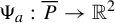 $\Psi _a : \overline P \to \mathbb {R}^2$
such that
 $\Psi _a(c) = 0$
and
 $\Psi _a$
conjugates the action of g on
 $\overline P$
to
 $$ \begin{align} (x,y) \mapsto \pm \bigg(\frac{x}{a}, ay \bigg), \end{align} $$
where the minus sign occurs if and only if c corresponds to a twisted orbit, and such that:
-
• if c is untwisted, the singularities of
$Q_0$
map to
$\pm (1,1)$
; and -
• if c is twisted, then one singular corner of
$Q_0$
maps to
$(1,1)$
and the other maps to a point
$(x,y)$
, for some
$x,y$
such that
$-a \le x,y \le -1/a$
.


Proof. Let
 $\ell ^v, \ell ^h$
be the vertical and horizontal leaves (that is, leaves of
 $\mathcal F^{s/u}$
) through c. By definition, the vertical/horizontal leaves through each point of
 $\overline P$
meet
 $\ell ^{h/v}$
, giving a coordinate system on
 $\overline P$
once we have chosen identifications of both
 $\ell ^v, \ell ^h$
with
 $\mathbb {R}$
.
If c is untwisted, then the dynamics of the action of
 $\pi _1(M)$
on
 $\mathcal {P}$
allow us to choose homeomorphisms of each half leaf
 $\ell ^{v}_{\pm }$
(respectively
 $\ell ^h_{\pm }$
) at c with
 $\mathbb {R}_{\ge 0}$
, which conjugate the action of g with multiplication by a (respectively
 $1/a$
), so that the associated function
 $\overline P\to \mathbb {R}^2$
maps the corners of
 $Q_0$
to
 $(\pm 1, \pm 1)$
.
In the twisted case, we first send the half leaf
 $\ell ^v_+$
to
 $\mathbb {R}$
via a map
 $f^v$
so that the point of intersection between
 $\ell _v^+$
and the vertical boundary of
 $Q_0$
goes to
 $1$
and so that the action of
 $g^2$
is conjugated to multiplication by
 $a^2$
. Then we define the map on
 $\ell ^v_-$
by
 $p \mapsto -a \; f^v(g^{-1}p)$
. The symmetric procedure for the horizontal leaf produces the required coordinates.
In both the twisted and untwisted cases, we call
 $Q_0$
the normalizing rectangle for the coordinates given by
 $\Psi _a$
. We fix a particular normalizing rectangle
 $Q_0$
.
For any
 $a>1$
, and every edge rectangle Q in P, we can draw a straight line
 $\gamma _Q$
in the
 $\Psi _a$
-coordinates on
 $\overline P$
connecting the singularities of Q. Identifying
 $\overline P$
with its image under
 $\Psi _a$
, we define
 $\alpha _a(Q)$
to be the point of intersection between
 $\gamma _Q$
and the x-axis (that is, the horizontal leaf through c). For all Q in P, we have
 $\alpha _a(g\cdot Q)=g\cdot \alpha _a(Q)$
since g preserves straight lines in
 $\Psi _a$
-coordinates.
Claim 5.9. There exists
 $a>1$
such that for each edge rectangle Q in P, the point
 $\alpha _a(Q)$
lies in the core box
 $b(Q)$
.
Proof. By Lemma 4.5, the action of
 $\pi _1(M)$
on the set of all edge rectangles is cofinite. If two elements of P are related by an element of
 $\pi _1(M)$
, then this element must lie in the stabilizer of c, which is equal to
 $\langle g\rangle $
. It follows that the action of
 $\langle g\rangle $
on P is cofinite.
Let Q be an edge rectangle of P. We claim that as
 $a\to 1^+$
,
 $\alpha _a(Q)\to c$
. To see this, first note that since c is g-invariant, it suffices to prove the claim for any g-translate of Q. Because the action of
 $\langle g\rangle $
on P is cofinite, each Q has a translate lying between
 $Q_0$
and
 $g^kQ_0$
for some k, not depending on Q, and so we replace Q with this translate. Then using the description of the action of g in
 $\Psi _a$
-coordinates from equation (5.2), we observe that
 $\Psi _a(g^kQ_0)$
(and
 $\Psi _a(Q_0)$
) converge to the square with corners at
 $(\pm 1, \pm 1)$
as
 $a \to \infty $
. In the case where c is twisted, this uses the fact (Claim 5.8) that when a is close to
 $1$
, the singular corner of the normalizing rectangle
 $Q_0$
in the negative quadrant is approaching
 $(-1,-1)$
. Since Q is above
 $Q_0$
and below
 $g^kQ_0$
, we also must have the same for
 $\Psi _a(Q)$
and we conclude that
 $\alpha _a(Q)\to c$
as
 $a\to 1^+$
.
Next, let
 $Q_1,\ldots Q_n$
be elements of P that together represent each g-orbit. We see that there exists an
 $a>1$
such that
 $\alpha _a(Q_i)\in b(Q_i)$
for
 $i=1,\ldots , n$
since c lies in the interior of each core box. Since the collection of core boxes is equivariant, this implies that
 $\alpha _a(Q)\in b(Q)$
for all Q in the preimage P.
Now fix such an
 $a>1$
, and define
 $\alpha (Q)=\alpha _a(Q)$
for all Q in the preimage P.
We can perform this procedure for an orbit representative of each pinched preimage, and extend to all pinched preimages by
 $\pi _1(M)$
-equivariance. Since each edge rectangle Q is either unpinched or is contained in a unique pinched preimage, this equivariantly assigns a point
 $\alpha (Q)$
to each edge rectangle Q. Set
 $A = \{\alpha (Q)\}$
, where Q varies over all edge rectangles.
Lemma 5.10. The pair
 $(\alpha , A)$
is an anchor system.
Proof. It only remains to prove monotonicity in staircases, that is, for edge rectangles
 $Q_1$
and
 $Q_2$
that share a singular corner s, if
 $Q_1$
is wider than
 $Q_2$
and
 $a_i=\alpha (Q_i)$
, then
 $R(s,a_1)$
is wider and no taller than
 $R(s,a_2)$
. We assume without loss of generality that
 $Q_1$
and
 $Q_2$
are right veering, and for convenience we identify the orthant of s determined by the
 $Q_i$
with the first quadrant of
 $\mathbb {R}^2$
.
By Lemma 5.5, monotonicity can only fail if
 $Q_1$
and
 $Q_2$
share a core point c. In this case,
 $Q_1$
and
 $Q_2$
lie in the same pinched preimage P, and we can consider these edge rectangles in the coordinates
 $\Psi _a$
where their
 $\alpha $
-values were chosen. In this case, since
 $Q_1$
is wider than
 $Q_2$
, and
 $\gamma _{Q_1}$
and
 $\gamma _{Q_2}$
are line segments with disjoint interiors, we see
 $a_1$
lies east of
 $a_2$
. This immediately implies that
 $R(s,a_1)$
is wider than
 $R(s,a_2)$
and the proof is complete.
Lemmas 5.3 and 5.10 together complete the proof of Proposition 5.2.
With Proposition 5.2 in hand, we can produce the fibration p.
Proposition 5.11. There exists a
 $\pi _1$
-equivariant fibration
 $p: \widetilde N \to \mathring {\mathcal {P}}$
whose restriction to each face of
 $\widetilde \tau $
is an orientation-preserving embedding into its associated rectangle.
The fibers of p are then oriented lines and the quotient by
 $\pi _1$
yields an oriented one-dimensional foliation positively transverse to
 $\tau ^{(2)}$
.
Proof. Fix an equivariant family of veering diagonals, as determined by Proposition 5.2. For each edge of e of
 $\widetilde \tau $
, map e homeomorphically to the veering diagonal associated to its edge rectangle. We choose these maps to be equivariant with respect to the
 $\pi _1(M)$
action.
If f is a face of
 $\widetilde \tau $
, then the edges in
 $\partial f$
are mapped to veering diagonals with disjoint interiors. Hence, we can equivariantly extend our map so that its restriction to each face is an orientation-preserving embedding. Finally, we extend our map equivariantly over each tetrahedron of
 $\widetilde \tau $
, as in Figure 19. In particular, the fibers of the projection in each tetrahedron are compact intervals that degenerate to points at the angle-
 $0$
edges. Using the local picture around faces and edges of
 $\widetilde \tau $
, we see that the resulting map
 $p : \widetilde N \to \mathring {\mathcal P}$
is a fibration.
5.6 Step 2: the fiberwise map
We begin by compactifying N to
 $\overline N$
and extending the foliation to the boundary components. This will allow us to realize this extension of diagram (5.1):

Here,
 is a renamed
 $\widetilde {\overline M}$
, the universal cover of
 $\overline M$
, while
 $\widehat M$
is the completion of the universal cover
 $\widetilde M$
, with the metric induced from the inclusion
 $M\hookrightarrow \overline M$
and any fixed metric on
 $\overline M$
. Note that
 is an infinite branched covering, to which the flow
 $\varphi $
lifts, and that the components of the completion locus are the preimages of singular orbits (we refer to these as the singular orbits of
 $\widehat M$
). Hence, the map to the flow space
 $\widetilde M \to \mathring {\mathcal P}$
extends equivariantly to a map
 $\widehat M \to \mathcal P$
.
On the left side of the diagram, we compactify N to
 $\overline N$
by adding torus boundary components (done carefully below so as to extend the foliation by p-fibers). We then let
 $\widehat N \to \overline N$
be the universal cover, with the intermediate cover
 obtained as that associated to
 $\ker (\pi _1(\overline N) \to \pi _1(\overline M))$
.
The compactification of N is carried out equivariantly on each tetrahedron
 $\kappa $
of
 $\widetilde N$
. Each ideal vertex of
 $\kappa $
has a neighborhood of the form
 $\Delta \times (0,1)$
, where
 $\Delta $
is a cross-sectional triangle, and moreover the foliation by p-fibers can be taken to be the same on each slice
 $\Delta \times \{t\}$
. To see this, note that p maps such a neighborhood to a region in
 $\mathring {\mathcal P}$
bounded between two veering diagonals, which can be written as an arc cross
 $(0,1)$
. The p-preimage of each arc is a cross-sectional triangle foliated by arcs.
We can therefore compactify
 $\kappa $
by adding a triangle
 $\Delta \times \{0\}$
for each ideal vertex, so that a neighborhood of
 $\Delta $
is of the form
 $\Delta \times [0,1)$
, and the map p extends to the added faces. We call the resulting polytope
 $\overline \kappa $
and refer to the added faces as cusp triangles. Doing this equivariantly, these compactifed tetrahedra glue together along hexagonal faces so that the quotient is a compactification
 $\overline N$
of N which is homeomorphic to N minus an open neighborhood of each cusp. We denote by
 $\widehat N$
the universal cover of
 $\overline N$
cellulated by the polytopes
 $\overline \kappa $
as above.
By construction, the foliation by p-fibers in
 $\widetilde N$
equivariantly extends to a foliation of
 $\widehat N$
by lines and we refer to the leaves of this foliation as p-leaves. We assign to each compactified tetrahedron
 $\overline \kappa $
a fixed continuously varying metric along its p-leaf segments which induces a continuously varying leafwise metric in
 $\overline N$
.
5.6.1 Defining an initial map
We next construct a preliminary
 $\pi _1$
-equivariant map
 $\widehat h : \widehat N \to \widehat M$
whose restriction
 $\widetilde h : \widetilde N \to \widetilde M$
commutes with the projections to the flow space
 $\mathring {\mathcal P}$
. In fact,
 $\widehat h : \widehat N \to \widehat M$
will commute with the natural projections to
 $\mathcal P$
, as we will soon see.
The p-leaves in
 $\widetilde N$
, together with their orientations and metric as given above, can be identified with
 $\mathbb {R}$
up to translation, and the same holds for the leaves of the flow in
 $\widetilde M$
.
Lemma 5.12. There exists a
 $\pi _1$
-equivariant map
 $\widehat h : \widehat N \to \widehat M$
whose restriction
 $\widetilde h : \widetilde N \to \widetilde M$
commutes with the projections to the flow space
 $\mathring {\mathcal P}$
so that for each p-leaf
 $\ell $
in
 $\widehat N$
, the restriction
 $\widehat h|_{\ell }$
, viewed as a map of oriented lines, is a degree
 $1 \ (a,b)$
-quasi-isometry, where a and b are independent of the leaf.
Proof. We construct
 $\widehat h$
successively on the skeleta of the completed 2-skeleton of
 $\widetilde \tau $
. For each
 $\tau $
-edge e of
 $\widetilde N$
, the projection
 $p(e)$
in
 $\mathring {\mathcal P}$
is a diagonal whose closure in
 $\mathcal P$
is an arc
 $\overline {p(e)}$
with endpoints at singularities. The restriction of the line bundle
 $\widehat M \to \mathcal P$
to
 $\overline {p(e)}$
is a trivial bundle, so we can choose a lift of
 $\overline {p(e)}$
(that is, a section of the bundle) whose endpoints are on singular orbits of
 $\widehat M$
. Thus, we have defined
 $\widehat h$
on a closed edge of
 $\widehat N$
whose interior is an edge of
 $\widetilde N$
. We do this for an edge in each
 $\pi _1$
-orbit and extend equivariantly. For any edge c of a cusp triangle
 $\Delta $
, we note that
 $\widehat h(\partial c)$
are two points in a single singular orbit of
 $\widehat M$
and so we extend
 $\widehat h$
over c by mapping it to the segment of the singular orbit joining its endpoints. This defines
 $\widehat h$
on
 $\widehat N^{(1)}$
in a
 $\pi _1$
-equivariant way.
The extension over
 $\tau $
-faces of
 $\widehat N$
is similar. For a face F of
 $\widetilde \tau ^{(2)}$
, its compactification
 $\overline F$
in
 $\widehat N$
is a hexagonal face of
 $\widehat N$
. The embedding
 $F \to p(F)$
extends to a map
 $\overline F \to \overline {p(F)}$
that collapses the edges of
 $\overline F$
contained in cusp triangles to the corresponding singular points of
 $\mathcal P$
. Pulling back the line bundle
 $\widehat M \to \mathcal P$
to
 $\overline F$
under this map allows us to extend the section already defined on
 $\overline F^{(1)}$
to
 $\overline F$
. We use this section of the pullback bundle to extend
 $\widehat h$
over
 $\overline F$
. Note that the restriction to F commutes with the projections to
 $\mathcal P$
by construction. Again, we extend over a face in each
 $\pi _1$
-orbit and extend equivariantly. This defines
 $\widehat h$
on the closures of the
 $\tau $
-faces in
 $\widehat N$
.
Finally, we extend the map
 $\widehat h$
continuously to the p-leaf segments. That is, for any leaf segment
 $\alpha $
in a compactified tetrahedron
 $\overline \kappa $
, its endpoints
 $\partial \alpha $
are in the compactified part of the
 $2$
-skeleton where
 $\hat h$
has already been defined and commutes with the projections to
 $\mathcal P$
. In particular, both endpoints of
 $\alpha $
map to the same leaf of the flow in
 $\widehat M$
, so that we may extend
 $\widehat h$
to a constant-speed map from
 $\alpha $
to that leaf. This completes the construction of
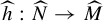 $\widehat h : \widehat N \to \widehat M$
with the required properties.
Equivariance means that
 $\widehat h$
descends to a continuous map
 $\overline h : \overline N \to \overline M$
, which maps each boundary torus of
 $\overline N$
to a singular orbit of
 $\overline M$
. We then lift
 $\overline h$
to
 , completing diagram (5.3). Properness of the deck group
 $\pi _1(\overline M)$
acting on
 and compactness of
 $\overline N$
together imply that
 is proper. (Note by comparison that
 $\widehat h$
is not proper—the preimage of a singular leaf in
 $\widehat M$
is a plane in
 $\widehat N$
, whereas the preimage of a singular leaf in
 is an annulus in
 ; this is why we need
 ).
We can now complete the proof of Lemma 5.12 by proving that
 $\widehat h$
has the required properties.
Coarse Lipschitz. This follows immediately from compactness of
 $\overline N$
and continuity of
 $\widehat h$
.
Uniform properness. Consider the lifted map
 . Every leaf in
 is properly embedded—indeed, as we know, the universal cover is a product whose vertical factors are the leaves. The same is true in
 : here, by construction, each leaf meets an infinite non-repeating sequence of cells of the triangulation, and since these are discrete in
 , the leaf must be properly embedded. Now, since as above
 is a proper map, its restriction to any leaf must be proper.
Moreover, the map is uniformly proper on leaves. For any point z in
 , let K be a compact neighborhood. The preimage of K is a compact set
 $K'$
, so for all leaves m passing through K, the preimage of
 $m\cap K$
is contained in
 $K'$
. This implies that the diameter in a leaf of the preimage of a segment in K is uniformly bounded. After covering a fundamental domain by finitely many such neighborhoods, we deduce that for any leaf segment in
 with diameter less than (say)
 $1$
, there is a uniform bound on the diameter of its preimage by
 . This implies uniform properness over all leaves.
Degree
 $1$
. We now check that
 has degree
 $1$
for for every leaf. That is, we must check that the ‘upward’ direction along leaves of
 maps to the ‘upward’ direction along orbits of
 , at large scale.
The coorientations on the faces of the tetrahedra in
 $\widetilde N$
(from §4.1) and the p-fibers were chosen so that when a leaf passes from a tetrahedron t to
 $t'$
in the forward direction,
 $t'$
lies above t, and this means that the rectangle of
 $t'$
is above that of t in the sense of §4.
Fact 5.13. Suppose that t and
 $t'$
are adjacent tetrahedra of
 $\widetilde N$
such that t lies below
 $t'$
in the sense that there is an oriented p-leaf passing from t to
 $t'$
. Then the maximal rectangle associated to t lies below the maximal rectangle associated to
 $t'$
.
This fact follows from considering the (finitely many) diagrams of a pair of adjacent tetrahedra. Now consider the sequence of tetrahedra that a forward ray of
 $\ell $
visits. Discreteness of the rectangles of
 $\mathring {\mathcal P} $
implies that these rectangles must have widths going to 0 and heights going to
 $\infty $
, in the sense of Fact 4.4.
However, consider a leaf of the flow in
 $\widetilde M$
. Fix an equivariant collection of sections of
 $\widetilde M \to \mathring {\mathcal P}$
over maximal rectangles as in Lemma 4.3. The sequence of rectangles met by a forward flow ray must, by Lemma 4.3, be eventually ordered with later ones lying above earlier ones.
Thus, upward motion in the leaves of both
 $\widetilde N$
and
 $\widetilde M$
corresponds to the same behavior of rectangles. Now to connect the two via
 $\widehat h$
, note that for each face F of
 $\widetilde \tau $
, the restriction of
 $\widehat h$
to F can be pushed along the flow in
 $\widetilde M$
until it meets the selected section of the rectangle associated to F. The distance along the flow required for this is uniformly bounded, since there are only finitely many orbits of faces. It follows, using properness of the map on leaves, that if an upward ray in
 $\widetilde N$
meets a sequence of faces
 $F_1,\ldots ,$
then its
 $\widetilde h$
image meets all but finitely many of the associated rectangle sections. Thus, upward rays map to upward rays. The same idea applies to downward rays.
Quasi-isometry. To finish, we need a lower bound on distances in the image. Identifying both
 $\ell $
and
 $\widehat h(\ell )$
with
 $\mathbb {R}$
in a length- and orientation-preserving way, it suffices to prove the following. There exists
 $A>0$
independent of
 $\ell $
such that for any
 $x,y\in \ell $
,
 $$ \begin{align} y> x+A \!\implies\! \widehat h|_{\ell}(y) > \widehat h|_{\ell}(x) + 1. \end{align} $$
Uniform properness implies that there exists
 $A>0$
, independent of
 $\ell $
and x, such that
 $y>x+A$
implies the distance between
 $\widehat h|_{\ell }(y)$
and
 $\widehat h|_{\ell }(x)$
is greater than 1. Degree 1 implies that, in fact,
 $\widehat h|_{\ell }(y)$
lies above
 $\widehat h|_{\ell }(x)$
in the orientation of the image leaf. This implies equation (5.4). This (together with coarse-Lipschitz above) suffices to prove that
 $\widehat h|_{\ell }$
is a quasi-isometry. This completes the proof of Lemma 5.12.
5.7 Step 3: straightening by convolution
We are now ready to obtain the homeomorphism.
Proposition 5.14. There is a
 $\pi _1$
-equivariant orientation-preserving homeomorphism
 $\widetilde f : \widetilde N\to \widetilde M$
which commutes with the fibrations
 $p : \widetilde N \to \mathring {\mathcal P}$
and
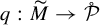 $q: \widetilde M \to \mathring {\mathcal P}$
.
Once we have this, we will denote by
 $f : N \to M$
the homeomorphism obtained by passing to the quotients. It follows easily that
 $f(\tau ^{(2)})$
is ‘topologically transverse’ to the flow
 $\varphi $
—see Proposition 5.15. Although this is all that we will need in practice, we will show in Step
 $4$
that this can be promoted to a smooth branched surface transverse to the flow.
Proof. The idea now is to convolve
 $\widetilde h|_{\ell }$
(for each leaf
 $\ell $
) with a bump function to get the desired map.
Let A be the constant in property (5.4) in the proof of Lemma 5.12. Let
 $\rho $
be a smooth bump function on
 $\mathbb {R}$
satisfying:
 $\rho \ge 0$
,
 $\int \rho = 1$
,
 $\rho $
is supported on
 $\{|x|\le A+1\}$
and constant on
 $[-A,A]$
,
 $\rho $
is even (
 $\rho (-x) = \rho (x)$
), and increasing on
 $[-A-1,-A]$
.
Now if
 $k:\mathbb {R}\to \mathbb {R}$
is a continuous map, we form
 $\rho \star k(t) = \int k(y) \rho (t-y) \,dy$
, which has the following properties.
-
(1)
$\rho \star k$
is differentiable. -
(2)
$\rho \star $
commutes with translations. That is, if
$T(x) = x+a$
, then
$\rho \star (f\circ T) = (\rho \star f)\circ T$
, and
$\rho \star (T\circ f) = T\circ (\rho \star f)$
. -
(3)
$\rho \star $
is continuous with respect to the compact-open topology on
$C(\mathbb {R},\mathbb {R})$
. -
(4) If k satisfies property (5.4), then
$(\rho \star k)'> \varepsilon >0$
, where
$\varepsilon $
depends only on
$\rho $
. -
(5) If
$k $
is
$(K,\delta )$
-coarse Lipschitz, then
$(\rho \star k)' < c$
, where c depends on
$\rho , K$
, and
$\delta $
. -
(6) If
$k $
is
$(K,\delta )$
-coarse Lipschitz, then
$| \rho \star k - k| < c$
, where c depends on
$\rho , K$
, and
$\delta $
.








Properties (1), (2), and (3) are standard. Properties (4) and (5) follow from the fact that given the properties of
 $\rho $
,
 $$ \begin{align*} (\rho\star k)'(t) = \int_A^{A+1} (k(t+u)-k(t-u)) |\rho'(u)|\,du, \end{align*} $$
which is easily verified. Property (6) is also a consequence of the averaging properties of convolution.
Translation-invariance implies that this convolution operation is well defined on the maps
 $\widetilde h|_{\ell }$
, because our identification of the leaves with
 $\mathbb {R}$
is well defined up to translation. We let
 $\rho \star \widetilde h$
denote this operation carried out simultaneously on all the leaves in
 $\widetilde N$
. Continuity property (3), and the continuity of
 $\widetilde h$
and the leafwise metrics that we chose in
 $\widetilde N$
, imply that the result is a continuous map.
By Lemma 5.12, each leafwise
 $\widetilde h|_{\ell }$
is coarse Lipschitz (with uniform constants) and satisfies equation (5.4). Thus,
 $\rho \star \widetilde h$
has positive derivative on each leaf, so it is a homeomorphism on leaves, and it is a bounded distance from
 $\widetilde h$
along the leaves (and, in particular, the two maps are homotopic). On the leaf space, the map is the identity, so it is globally a homeomorphism from
 $\widetilde N$
to
 $\widetilde M$
which commutes with the projections to the leaf space.
Finally,
 $\rho \star \widetilde h$
is equivariant: since the group acts by orientation-preserving isometries on the leaves both in
 $\widetilde N$
and
 $\widetilde M$
, this follows from equivariance of
 $\widetilde h$
and translation-invariance of
 $\rho \star $
. This completes the proof.
We can now state an immediate application of Proposition 5.14, which is the topological version of our main result, Theorem 5.1.
Proposition 5.15. There is a homeomorphism
 $f: N \to M$
, inducing the identity on
 $\pi _1(M)$
, such that the image of
 $\tau ^{(2)}$
is a cooriented branched surface that is topologically positively transverse to flow lines of
 $\varphi $
.
Here, by ‘topologically positively transverse,’ we mean that the image of
 $\tau ^{(2)}$
has a branched surface fibered neighborhood whose oriented fibers are segments of flow lines.
5.8 Step 4: smoothing
The next proposition completes the proof of Theorem 5.1.
Proposition 5.16. The homeomorphism
 $f : N \to M$
from Proposition 5.15 can be chosen so that
 $f(\tau ^{(2)})$
is a smooth branched surface which is positively transverse to flow lines of
 $\varphi $
.
Proof. We will indicate how the previous construction can be adjusted so as to yield a smooth result. The first step is to give the line bundle
 $\widetilde N \to \mathring {\mathcal P}$
a smooth structure with respect to which sections carried by the branched surface are smooth.
Since the flow is smooth off its singular orbits, the flow space
 $\mathring {\mathcal P}$
inherits a smooth structure from M. After a small equivariant perturbation, we may assume that the diagonals are smooth and that triangles are still embedded. (The diagonals may no longer be transverse to the stable/unstable foliations, but they are still contained in their respective edge rectangles—we will improve this in Proposition 5.17).
Next we need to specify the fiberwise metrics on the p-leaves so that they vary smoothly with respect to the base. Each p-leaf is composed of segments from the foliation of the tetrahedra. We can metrize these segments in each tetrahedron (equivariantly) so that their lengths vary smoothly and converge to
 $0$
at the
 $0$
-angle edges of the tetrahedron, and have derivatives
 $0$
there (we can make higher derivatives match across the edge for greater smoothness).
This allows us to give local trivializations of the bundle
 $p: \widetilde N \to \mathring {\mathcal P}$
. Over a small disk, consider a section that lies in the branched surface and use the metric on leaves to define a trivialization where that section is at constant height. The way we chose the fiber segment lengths implies that different choices of sections give trivializations for which transition maps are smooth. Thus we have a smooth structure on the bundle for which sections lying in the branched surface are smooth.
When we define the map
 $\widehat h$
, we first choose sections over the veering edges. These can be chosen smoothly on the interiors of the edges. We then extend to the faces of
 $\widetilde {\tau }^{(2)}$
smoothly, and in such a way that the sections are tangent to each other at the edges. The extension of
 $\widehat h$
to the p-leaf segments in each tetrahedron can be done at constant speed, so that since the maps on the endpoints are smooth by the previous paragraph, we find that in a local trivialization of p, the map varies smoothly with respect to the coordinates in
 $\mathring {\mathcal P}$
. Note that we do not obtain smoothness of
 $\widehat h$
on the completion points of
 $\widehat N$
, but we only need continuity there.
The map, which may still not be injective or smooth in the fiber direction, is now averaged in the convolution step. The final map is smooth in the fiberwise direction because the bump function
 $\rho $
is smooth, and it is smooth in the
 $\mathring {\mathcal P}$
direction because the fiberwise metrics and the map
 $\widetilde h$
are smooth with respect to the
 $\mathring {\mathcal P}$
direction. Thus, our final map is a diffeomorphism and the image of the branched surface is transverse to the flow.
5.9 Transversality in the flow space
In the interest of recovering as much of the picture as possible in the suspension flow case, we would also like the smooth veering edges in each edge rectangle in
 $\mathring {\mathcal P}$
to be transverse to both stable and unstable foliations. We note that this is not needed for the flow-transversality of Proposition 5.16.
Proposition 5.17. The fibration
 $p: \widetilde N \to \mathring {\mathcal P}$
can be chosen so that the images of the veering edges are smooth and transversal to both the stable and unstable foliations.
We note that this is easy if the stable and unstable foliations are at least
 $C^2$
, because then the rectangles can be smoothly identified with Euclidean rectangles foliated by axis-parallel lines. Our foliations may not have this regularity, although for dynamical reasons, they do have smooth leaves and line fields which are uniquely integrable. These facts are well known for Anosov flows [Reference AnosovAno63] and the proofs also apply more generally to pseudo-Anosov flows (see [Reference Fenley and MosherFM01]). This turns out to be enough.
The proposition will follow directly from Corollary 5.19.
In this section, by smooth, we mean at least
 $C^2$
. A smooth quadrilateral is a smooth disk-with-corners that has four corners and two transverse foliations, so that each foliation is tangent to two opposite boundary edges. We do not assume that the foliations themselves are smooth.
Such a quadrilateral has a diffeomorphism to the unit square, taking the two foliations to foliations that include the horizontal and vertical boundary edges, respectively. From now on, we identify Q with
 $[0,1]^2$
, we call the foliations
 $F_h$
and
 $F_v$
, and we say that a diagonal of Q is a path from
 $(0,0)$
to
 $(1,1)$
.
Lemma 5.18. Let Q be a smooth quadrilateral. If the line fields of
 $F_h$
and
 $F_v$
are uniquely integrable, then there exists a smooth diagonal which is transverse to both
 $F_h$
and
 $F_v$
. Moreover, one can prescribe the tangent direction of the diagonal at each of its endpoints.
We remark that the lemma is false without the unique integrability assumption, so that there really is something to do here.
As a corollary, we have the following.
Corollary 5.19. Let Q be a smooth quadrilateral for which the line fields of
 $F_h$
and
 $F_v$
are uniquely integrable, and
 $\alpha $
a continuous diagonal which is topologically transverse to both of the foliations. Then
 $\alpha $
can be
 $C^0$
approximated by a smooth diagonal transverse to both foliations.
Here, ‘topologically transverse’ means that the diagonal meets every foliation leaf exactly once.
Proof of Corollary 5.19
Subdivide
 $\alpha $
into small segments. Because it is topologically transverse, the endpoints of every segment are opposite corners for a foliated sub-quadrilateral, so that adjacent quadrilaterals meet exactly at their common corner. We may choose tangent lines at every corner which point into the two adjacent quadrilaterals, and then use Lemma 5.18 to find a smooth diagonal for each quadrilateral matching the given tangent direction at the corners. These piece together to a
 $C^1$
diagonal which is transverse to both foliations and closely approximates
 $\alpha $
in
 $C^0$
. A further (standard) smoothing step upgrades this to a smooth diagonal.
Proof of Lemma 5.18
We will need this calculus lemma, whose proof we omit.
Lemma 5.20. Let
 $\alpha _n:[0,1] \to \mathbb {R}^d$
be
 $C^1$
curves. Suppose that
 $\alpha _n \to \alpha $
pointwise, and
 $\alpha ^{\prime }_n$
converges to a continuous vector field u along
 $\alpha $
. Suppose moreover that all the functions
 $t\mapsto \alpha ^{\prime }_n(t)$
have a common modulus of continuity. Then
 $\alpha $
is differentiable and
 $\alpha ' = u$
.
Now we apply this to our setting. Let
 $u,v$
be
 $C^0$
vector fields on Q that are tangent to
 $F_h$
and
 $F_v$
, respectively. Extend
 $u,v$
continuously to a small neighborhood of Q, and form the open tangent cone field C, where
 $C(x) = \{au(x)+bv(x) : a,b>0\}$
. Given any fixed
 $a,b>0$
, the vector field
 $au+bv$
lies in C, and varying over convex combinations
 $a+b=1$
, we obtain a family of vector fields with a common modulus of continuity.
Let
 $\rho _a(x)$
be a family of bump functions varying smoothly with
 $a\in (0,1)$
, with mass 1 and support of size
 $\varepsilon (a)$
, such that
 $\varepsilon \to 0$
smoothly as
 $a\to 0$
or
 $a\to 1$
. If the function
 $\varepsilon $
is chosen small enough, then, convolving
 $au+bv$
with
 $\rho _a$
, we get a family of smooth vector fields
 $\xi _a$
on Q in the cone field C, all with a common modulus of continuity, such that
 $\xi _a \to u$
as
 $a\to 1$
and
 $\xi _a \to v$
as
 $a\to 0$
.
Now for each
 $a\in (0,1)$
, smoothness implies
 $\xi _a$
is uniquely integrable so let
 $\alpha _a$
be an integral curve starting at the lower-left corner of Q. Thus,
 $\alpha _a$
satisfies
 $\alpha _a'(t) = \xi _a(\alpha _a(t)) \in C(\alpha _a(t))$
for any t for which the curve is defined. In fact (since
 $\xi _a$
is smooth), this is defined until it leaves Q, and this must be on the right or top edge since C points into Q at points of the left and bottom edges.
Now we can take the limit as
 $a\to 0$
. Because
 $\alpha _a$
have bounded derivatives, Arzelà–Ascoli gives us some sequence
 $a_n\to 0$
for which the curves converge to some limit curve
 $\alpha _0$
. We know that the vector fields
 $\alpha ^{\prime }_a(t)$
along the curves satisfy a common modulus of continuity because
 $\xi _a$
do, and the
 $\alpha _a$
have bounded speed. Thus, Lemma 5.20 applies to tell us that
 $\alpha _0$
is differentiable and its derivative is just the limit of
 $\xi _a$
(restricted to
 $\alpha _0$
) which is the vector field v. That is,
 $\alpha _0$
is an integral curve of v starting at the lower left corner, and hence the left-boundary leaf of the foliation
 $F_v$
by unique integrability. This means
 $\alpha _0$
terminates on the upper left corner.
Similarly a limit as
 $a \to 1$
gives
 $\alpha _1$
which terminates on the lower right corner.
Continuity gives us a value of a for which
 $\alpha _a$
terminates on the upper-right corner.
Once we have the desired path
 $\alpha _a$
, we need to perturb it so that it has the desired tangent directions at the corners. This is more simple: the vector fields u and v are continuous at the corners. So in a small enough neighborhood of (say) the corner
 $(0,0)$
, they are much closer to the coordinate vector fields than they are to the direction of
 $\alpha _a$
. Now, thinking of
 $\alpha _a$
as the graph of a function, add a smooth function with small support near 0 and the appropriate derivative at 0.
6 The flow graph and orbits of the flow
Let
 $\varphi $
be a pseudo-Anosov flow without perfect fits on
 $\overline M$
and let
 $\tau $
be the veering triangulation of
 $M = \overline M \smallsetminus \{\text {singular orbits}\}$
dual to
 $\varphi $
. In this section, we detail how the flow graph
 $\Phi $
uniformly codes orbits of the flow
 $\varphi $
.
Recall that
 $\mathcal O_{\varphi }^+ \subset M$
is the union of closed orbits
 $\mathcal O_{\varphi }$
of the flow along with all positive multiples of unstable prong curves in M. We also denote by
 $\mathcal {Z}_{\Phi }$
the set of directed cycles of
 $\Phi $
. In §6.3, we produce a map
 $$\begin{align*}{\mathfrak F} : \mathcal{Z}_{\Phi} \to \mathcal O_{\varphi}^+, \end{align*}$$
with the property that the directed cycle c is homotopic to
 ${\mathfrak F}(c)$
in M. We remark that when
 ${\mathfrak F}(c)$
is non-singular (i.e. a closed orbit in M; not a prong curve), it is the unique closed orbit of
 $\varphi $
homotopic to the flow cycle c.
The main theorem of this section (proven in §6.3) is a summary of the essential features of the map
 ${\mathfrak F}$
. For its statement, we need one additional definition. Let
 $\gamma _1$
and
 $\gamma _2$
be two directed closed curves in M which are positively transverse to
 $\tau ^{(2)}$
. We say that
 $\gamma _1$
and
 $\gamma _2$
are transversely homotopic if they are homotopic through closed curves that are positively transverse to
 $\tau ^{(2)}$
.
We also remind the reader that
 $\delta _{\tau }$
denotes the length of the longest fan in
 $\tau $
.
Theorem 6.1. (Closed orbits and the flow graph)
The map
 ${\mathfrak F} : \mathcal Z_{\Phi } \to \mathcal O_{\varphi }^+$
has the following properties.
-
(1) The image
$\gamma = {\mathfrak F}(c)$
, which is either a non-singular closed orbit of
$\varphi $
or an unstable prong curve, is transversely homotopic to c in M. -
(2) For each unstable prong curve
$\gamma $
,
$1 \le \# \mathfrak F^{-1}(\gamma ) \le 2$
. -
(3) For each non-singular closed orbit
$\gamma $
of
$\varphi $
, either
$\# \mathfrak F^{-1}(\gamma ) \le 1$
or
$\gamma $
is homotopic to an
$AB$
-cycle, in which case,
$\# \mathfrak F^{-1}(\gamma ) \le \delta _{\tau }$
. -
(4) For each non-singular closed orbit
$\gamma $
of
$\varphi $
, either
$\gamma $
is in the image of
$\mathfrak F$
or
$\gamma $
is homotopic to an odd AB-cycle.


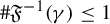


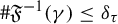


In short, the flow graph
 $\Phi $
encodes all but finitely many primitive orbits of the flow in a one-to-one fashion. We remark that simple cycles of
 $\Phi $
can map to non-primitive orbits of
 $\varphi $
; this happens, for example, in the presence of twisted orbits.
6.1 The flow space and the flow graph
We begin by explaining how the structure of
 $\Phi $
is recorded by the maximal rectangles of the completed flow space
 $\mathcal P$
.
By the construction of
 $\tau $
, each
 $\tau $
-edge e of the lifted triangulation
 $\widetilde \tau $
on
 $\widetilde M$
corresponds to a unique edge rectangle in
 $\mathcal P$
. Similarly, faces of
 $\widetilde \tau $
correspond to face rectangles and tetrahedra correspond to maximal rectangles. In fact, we can use Proposition 5.2 to fix a
 $\pi _1(M)$
-equivariant map
 $\widetilde M \to \mathcal P$
that embeds each
 $\tau $
-edge in its edge rectangle so that the restriction to each face of
 $\widetilde \tau $
is also an embedding. We fix such a map once and for all, and, abusing terminology, we will also refer to the image of e in
 $\mathcal P$
as a
 $\tau $
-edge. For example, a
 $\tau $
-edge e is contained in a maximal rectangle R if and only if its edge rectangle Q is contained in R. The singularities at the corners of Q are necessarily contained in the interiors of the sides of R.
If Q is the edge rectangle for a
 $\tau $
-edge e, then we denote by either
 $R_e$
or
 $R_Q$
the maximal rectangle obtained by extending Q vertically along leaves of
 $\mathcal F^{\kern1.3pt s}$
as far as possible, so that e joins its vertical sides. See Figure 24. In terms of the veering triangulation
 $\widetilde \tau $
of
 $\widetilde M$
,
 $R_e$
is the maximal rectangle corresponding to the tetrahedron having e as its bottom edge.
Vertically extending an edge rectangle (left, green) to a maximal rectangle (right, blue) (in colour online).

We also fix the inclusion
 $\iota : \Phi \to M$
in dual position. In this section, it will be convenient to identify
 $\Phi $
with its image under
 $\iota $
. Recall that in this position, the vertices of
 $\Phi $
agree with the vertices of the dual graph
 $\Gamma $
and hence with the triple points of the stable branched surface
 $B^s$
.
By [Reference Landry, Minsky and TaylorLMT20, Lemma 4.4],
 $\iota : \Phi \to M$
is
 $\pi _1$
-surjective and so the flow graph
 $\Phi $
has connected preimage in the universal cover of M, which we denote by
 $\widetilde \Phi $
. Identifying each
 $\tau $
-edge e with the maximal rectangle
 $R_e$
leads to the following alternative description of
 $\widetilde \Phi $
: the vertices of
 $\widetilde \Phi $
are maximal rectangles and for each maximal rectangle R, there are directed edges from
 $R=R_b$
to the three rectangles
 $R_t, R_{s_1}, R_{s_2}$
, where t is the
 $\tau $
-edge joining the horizontal sides of R, and
 $s_1$
and
 $s_2$
are
 $\tau $
-edges of R such that the rectangles
 $R_t, R_{s_1}, R_{s_2}$
have non-overlapping interiors (see Figure 25). This is to say that in the rectangle R, the set
 $t\cup s_1\cup s_2$
passes the ‘vertical line test.’ We will freely use this correspondence between
 $\widetilde \Phi $
-vertices and maximal rectangles.
The outward
 $\widetilde \Phi $
-edges of the
 $\tau $
-edge e in terms of maximal rectangles. The dotted lines indicate that those portions of the boundaries of rectangles do not meet (in colour online).

We similarly consider the preimage
 $\widetilde \Gamma $
of the dual graph
 $\Gamma $
in the universal cover of M. Each vertex of
 $\widetilde \Gamma $
is contained in the interior of a unique tetrahedron of
 $\widetilde M$
and hence also corresponds to a unique maximal rectangle. Understanding paths in
 $\widetilde \Gamma $
with this perspective is fairly straightforward.
Lemma 6.2. Let
 $R_1$
and
 $R_2$
be maximal rectangles in
 $\mathcal {P}$
and suppose that
 $R_2$
lies above
 $R_1$
. Let
 $v_1$
and
 $v_2$
be the
 $\widetilde \Gamma $
-vertices corresponding to
 $R_1$
and
 $R_2$
. Then there exists a directed
 $\widetilde \Gamma $
-path from
 $v_1$
to
 $v_2$
.
Proof. Let
 $T_1$
and
 $T_2$
be the
 $\widetilde \tau $
-tetrahedra corresponding to
 $R_1$
and
 $R_2$
, respectively. Since
 $R_2$
lies above
 $R_1$
, the projections of
 $T_1$
and
 $T_2$
to
 $\mathcal {P}$
must overlap. Hence, there is a
 $\widetilde \varphi $
-orbit passing through both
 $T_1$
and
 $T_2$
. Further observe that whenever an orbit passes from a tetrahedron
 $T_a$
to an adjacent tetrahedron
 $T_b$
, the maximal rectangle
 $R_a$
associated to
 $T_a$
lies below the maximal rectangle
 $R_b$
associated to
 $T_b$
(see Fact 5.13). Hence, the given orbit must pass first through the tetrahedron
 $T_1$
and then through the tetrahedron
 $T_2$
.
By truncating this orbit and adding small segments in
 $T_1$
and
 $T_2$
, we obtain a path from
 $v_1$
to
 $v_2$
which is positively transverse to
 $\widetilde \tau ^{(2)}$
. After perturbing rel endpoints to make it disjoint from
 $\widetilde \tau ^{(1)}$
, the sequence of
 $\widetilde \tau $
-faces traversed by this path corresponds to a directed
 $\widetilde \Gamma $
-path from
 $v_1$
to
 $v_2$
.
To understand directed paths in
 $\widetilde \Phi $
, it is convenient to work with the dynamic planes of §3, as we now explain.
A singular leaf of either the stable or unstable foliation of
 $\mathcal P$
is a leaf homeomorphic to
 $[0,\infty )$
with its endpoint on a singularity of
 $\mathcal P$
. A point p of
 $\mathcal P$
is a regular point if it does not lie in a singular leaf of either foliation. We remark that all fixed points of
 $\mathcal P$
under the
 $\pi _1(M)$
-action are either regular or singular, since singularities are the only fixed points in their stable/unstable leaves.
Now let
 $p\in \mathcal P$
be a regular point. A p-rectangle or maximal p-rectangle is a rectangle or maximal rectangle, respectively, which contains p in its interior. A p-ray is a directed infinite ray in
 $\widetilde \Phi $
traversing only maximal p-rectangles.
Lemma 6.3. Let R be a maximal p-rectangle for a regular point
 $p\in \mathcal P$
. There is a unique p-ray starting at R.
Proof. By definition, there are directed edges from
 $R=R_b$
to
 $R_{s_1},R_{s_2},R_t$
, where
 $R_{s_1},R_{s_2},R_t$
cover R and have disjoint interiors. Since p is a regular point, it is interior to exactly one of
 $R_{s_1},R_{s_2}, R_t$
. In other words, every maximal p-rectangle has a unique outgoing
 $\widetilde \Phi $
-edge connecting it to another maximal p-rectangle.
In the next proposition, we associate to each (singular) leaf
 $\ell $
of
 $\mathcal F^{\kern1.3pt s}$
a unique dynamic (half-) plane
 $D_{\ell }$
. As in §3.1, we denote by
 $\sigma (v)$
the unique sector of
 $\widetilde B^s$
whose top vertex is v. If R is the maximal rectangle of
 $\mathcal P$
corresponding to the vertex v of
 $\widetilde \Gamma $
, we extend this notation to
 $\sigma (R) = \sigma (v)$
. The reader can check that if e is an edge of
 $\widetilde \tau $
, then
 $\sigma (R_e)$
is the unique sector of
 $\widetilde B^s$
dual to e.
Proposition 6.4. (Dynamic planes for stable leaves)
Let
 $\ell $
be a (singular) leaf of the vertical foliation
 $\mathcal F^{\kern1.3pt s}$
. The union
 $$\begin{align*}D_{\ell} = \bigcup_{\ell \cap \mathrm{int}(R) \neq \emptyset} \sigma(R) \end{align*}$$
of all sectors of
 $\widetilde B^s$
associated to maximal rectangles R that meet
 $\ell $
in their interior is a dynamic (half-) plane.
Moreover,
 $D_{\ell }$
has the property that for any dual ray (or flow ray)
 $\widetilde \gamma $
whose vertices correspond to maximal rectangles that meet
 $\ell $
in their interior, we have
 $D_{\ell } = D(\widetilde \gamma )$
.
For the proof, we first define the dynamic (half-) plane associated to any increasing sequence of rectangles. Let
 $A=(A_1, A_2, A_3,\ldots )$
be any sequence of distinct maximal rectangles with the property that
 $A_{i+1}$
lies above
 $A_i$
for all i. We remark that A could be a path in
 $\widetilde \Gamma $
, in
 $\widetilde \Phi $
, or in neither, though only the
 $\widetilde \Gamma $
and
 $\widetilde \Phi $
cases are relevant for us.
By Lemma 6.2, there is a
 $\widetilde \Gamma $
-path from
 $A_i$
to
 $A_{i+1}$
for all i. The union of these
 $\widetilde \Gamma $
-paths gives a (possibly non-unique)
 $\widetilde \Gamma $
-ray
 $\gamma _A$
. It follows that A determines a dynamic (half-) plane
 $D_A$
, which can be defined by
 $$\begin{align*}D_A= D(\gamma_A) = \bigcup_{i} \Delta(\sigma(A_i)), \end{align*}$$
where
 $\Delta (\sigma )$
is the descending set of
 $\sigma $
, as is in §3.1. Note that the
 $\Delta (\sigma (A_i))$
form a nested union of descending sets by Lemma 3.3 and so
 $D_A$
is independent of the choice of
 $\gamma _A$
. Also,
 $D_A$
is a dynamic half-plane if and only if
 $\gamma _A$
is eventually a branch ray. In terms of rectangles, this is equivalent to the condition that there is a single singularity s such that either the top or bottom components of all
 $\partial _h A_i$
eventually contain s. To see this, first note that by Lemma 6.2, it suffices to assume that A is a sequence of consecutive maximal rectangles in the sense that
 $A_i$
and
 $A_{i+1}$
intersect along a face rectangle
 $F_i$
. Then from the picture in the flow space, one sees that there exists a singularity s eventually contained in all
 $\partial _h A_i$
if and only if it is eventually the case that the edge rectangle of intersection between
 $F_i$
and
 $F_{i+1}$
always has the opposite veer as the top edge rectangle of
 $A_{i+1}$
. This exactly characterizes branch rays; see for example [Reference Landry, Minsky and TaylorLMT20, Lemma 4.5].
Proof of Proposition 6.4
First fix an arbitrary maximal rectangle
 $A_0$
such that
 $\sigma (A_0)$
is a sector of
 $D_{\ell }$
, and a sequence
 $A=(A_0, A_1, A_2, A_3,\ldots )$
of distinct maximal rectangles meeting
 $\ell $
in their interiors with the property that
 $A_{i+1}$
lies above
 $A_i$
for all i. Note that
 $\ell $
is a singular leaf with singularity p if and only if
 $A_i$
contains p in its horizontal boundary for i sufficiently large. We will show that
 $D_{\ell } = D_A$
.
Next let
 $B_0$
be any maximal rectangle with
 $\sigma (B_0)$
a sector of
 $D_{\ell }$
and, as above, let
 $B=(B_0, B_1,B_2,B_3,\ldots )$
be another such sequence of maximal rectangles, determining a dynamic plane
 $D_B$
in the same way. We claim that
 $D_A=D_B$
. Indeed, let
 $A_i$
be a term of A. By the discreteness of singularities in
 $\mathcal {P}$
, there exists some j such that
 $B_j$
lies above
 $A_i$
(see Fact 4.4). By Lemma 6.2, there is a dual path from
 $A_i$
to
 $B_j$
, so by Lemma 3.3, we have
 $\Delta (\sigma (A_i))\subset \Delta (\sigma (B_j))$
. Since this holds for any rectangle in A, we see that
 $D_A\subset D_B$
. The proof of the reverse inclusion is the same, so we have the equality
 $D_A=D_B$
.
Since
 $B_0$
was an arbitrary maximal rectangle with
 $\sigma (B_0) \subset D_{\ell }$
, we conclude that
 $D_{\ell } \subset D_A$
. Moreover, since any rectangle R with
 $\sigma (R) \subset D_A$
lies below some
 $A_i$
, we also have that the interior of R meets
 $\ell $
. Hence,
 $D_A \subset D_{\ell }$
. This proves that
 $D_{\ell }$
is a dynamic (half-) plane. The moreover claim is now clear from the construction of
 $D_A$
and the equality
 $D_A = D_{\ell }$
.
For any point
 $p \in \mathcal P$
that is not a singularity, we further define
 $D_p = D_{\ell }$
, where
 $\ell $
is the unique leaf of
 $\mathcal F^{\kern1.3pt s}$
through p. The planes
 $D_{\ell }$
and
 $D_p$
are called the dynamic planes for
 $\ell $
and p, respectively.
Remark 6.5. Singular leaves and dynamic planes
If
 $\ell $
is leaf of
 $\mathcal F^{\kern1.3pt s}$
, then
 $\ell $
is singular if and only if
 $D_{\ell }$
is a dynamic half-plane. Moreover, in this case, any increasing sequence of rectangles
 $(A_i)$
whose terms all intersect
 $\ell $
in their interior has the property that the singular point p along
 $\ell $
is eventually contained in the horizontal boundary of
 $A_i$
for sufficiently large i.
In this situation, we can pick one of two sides of
 $\ell $
and extend along maximal rectangles which are contained in that side and which contain p in their vertical boundary (see Figure 26). The argument from the proof of Proposition 6.4 shows that doing so produces a unique dynamic plane containing
 $D_{\ell }$
. Since
 $\ell $
has two sides, this procedure produces two dynamic planes that contain
 $D_{\ell }$
. (In fact, these are the only two dynamic planes containing
 $D_{\ell }$
, but we will not need this.) Moreover, each of these dynamic planes is stabilized by the (necessarily non-trivial) stabilizers of
 $D_{\ell }$
.
A singular leaf
 $\ell $
with singularity p and an increasing sequence of maximal rectangles that intersect
 $\ell $
with the property that p is eventually contained in the vertical boundary of all terms. The resulting dynamic plane contains the dynamic half-plane
 $D_{\ell }$
(in colour online).

Proposition 6.4 implies that for each regular point
 $p\in \mathcal {P}$
, any two p-rays lie in the dynamic plane for p. Combining with Corollary 3.13 gives us the following lemma.
Lemma 6.6. Let
 $p\in \mathcal P$
be a regular point with dynamic plane D. The number of asymptotic classes of p-rays is equal to the width of D, and hence is at most
 $\delta _{\tau }$
.
With these results relating dynamic planes to the flow space in hand, we can now characterize when closed paths in M are transversely homotopic. This will be essential for the results in §7.
Proposition 6.7. (Transverse homotopies)
Let
 $\gamma _1$
and
 $\gamma _2$
be two homotopic closed curves which are positively transverse to
 $\tau ^{(2)}$
. Then either they are transverse homotopic or they are homotopic to branch curves.
Proof. We first perturb
 $\gamma _1$
and
 $\gamma _2$
to avoid
 $\tau ^{(1)}$
. Then each
 $\gamma _i$
determines a unique
 $\Gamma $
-cycle to which it is transversely homotopic. Hence, it suffices to prove the claim when
 $\gamma _1$
and
 $\gamma _2$
are
 $\Gamma $
-cycles. Assume that neither is homotopic to a branch curve.
Lifting a homotopy from
 $\gamma _1$
to
 $\gamma _2$
, we obtain
 $\Gamma $
-lines
 $\widetilde \gamma _1$
and
 $\widetilde \gamma _2$
that are stabilized by
 $\langle g \rangle \le \pi _1(M)$
. If we intersect the sequence of maximal rectangles associated to
 $\widetilde \gamma _1$
(or
 $\widetilde \gamma _2$
), we obtain a single
 $p\in \mathcal P$
by Fact 4.4. By construction, p is stabilized by g and so p is regular. Otherwise, p would necessarily be a singularity of
 $\mathcal P$
and
 $\gamma _1$
would be homotopic to a branch curve in the corresponding cusp of M.
Therefore, p determines a dynamic plane
 $D_p$
that contains
 $\widetilde \gamma _1$
and
 $\widetilde \gamma _2$
by Proposition 6.4. Applying Lemma 3.17, we see that
 $\gamma _1$
and
 $\gamma _2$
are homotopic by sweeping across sectors of
 $B^s$
. Since such homotopies are visibly through curves that are transverse to
 $\tau ^{(2)}$
(see Figure 27), the proof is complete.
Homotoping one side of a
 $B^s$
-sector to another through curves positively transverse to
 $\tau ^{(2)}$
(in colour online).

6.2 Lines of
$\widetilde \Phi $
and the flow

We now focus on associating to each directed line of the graph
 $\Phi $
an orbit of the flow
 $\varphi $
. More precisely, we define a map
 $$\begin{align*}\widetilde {\mathfrak F} : \{\text{directed lines in } \widetilde \Phi \} \to \mathcal P \end{align*}$$
from directed lines in
 $\widetilde \Phi \subset \widetilde M$
to the completed flow space
 $\mathcal P$
. Each directed line
 $\widetilde \gamma $
in
 $\widetilde \Phi $
corresponds to a sequence of maximal rectangles which become taller in the positive direction and wider in the negative direction. Then, as in Proposition 6.7, Fact 4.4 implies that the intersection of the rectangles in this sequence is a single point
 $\widetilde {\mathfrak F}(\widetilde \gamma ) \in \mathcal P$
. See Figure 28. It is not hard to see that this map is
 $\pi _1(M)$
-equivariant and continuous with respect to the usual topology on the space of lines.
The map
 $\widetilde {\mathfrak F}$
sends a
 $\widetilde \Phi $
-line, which corresponds to a certain bi-infinite sequence of maximal rectangles, to the unique point in
 $\mathcal {P}$
lying in all of the rectangles (in colour online).

To understand the image of
 $\widetilde {\mathfrak F}$
in
 $\mathcal P$
, we again study the structure of dynamic planes.
Define a chain of sectors in a dynamic plane D to be a union of sectors attached as in Figure 29. More precisely, a chain is a collection of sectors
 $\sigma _1,\ldots , \sigma _n$
such that an entire bottom branch segment of
 $\sigma _i$
is identified with a top branch segment of
 $\sigma _{i+1}$
for
 $i = 1,\ldots ,n-1$
, and there is a single branch segment that contains a top branch segment of each
 $\sigma _i$
for
 $i = 1,\ldots ,n$
, i.e. the union
 $\bigcup _{i=1}^n \sigma _i$
is bounded by four branch segments. Two of these are the top branch segments of the chain and two are the bottom. Note that every sector has two chains, possibly of length
 $1$
. When a chain has length at least
 $2$
, we say a branch segment in its boundary is long if it contains an edge of each sector of the chain and is short otherwise. See Figure 29 for an example.
A chain of length four. The highlighted branch segments are long, and the other two branch segments in the boundary of the chain are short. The vertices indicated by black dots all have the same veer by Lemma 3.8. Either of the two bottom branch segments could possibly have more vertices than shown (in colour online).

We now show that lengths of chains are uniformly bounded by
 $\delta = \delta _{\tau }$
, which, as a reminder, is the length of the longest fan of
 $\tau $
.
Lemma 6.8. Any chain of sectors in a dynamic plane has length less than
 $\delta $
.
Proof. Suppose that C is a chain of length
 $k\ge 2$
. An application of Lemma 3.8 shows that the bottom
 $k-1$
sectors of C have top and bottom vertices of the same veer. This means that the long top branch segment of C passes through
 $k-1$
consecutive non-hinge tetrahedra. Applying Claim 3.11 gives that these tetrahedra lie in the fan of a single edge. As in the proof of Proposition 3.10, we note that this implies the existence of a fan of length
 $k-1+2=k+1$
(see [Reference Futer and GuéritaudFG13, Observation 2.6]).
Recall that Lemma 3.7 says that flow rays converge in dynamic planes unless they are separated by AB strips. The next lemma essentially says that this convergence is rapid, and is key to proving Proposition 6.12, which says that
 $\widetilde {\mathfrak F}$
is surjective and uniformly finite-to-one away from singularities.
Lemma 6.9. Let
 $\sigma $
be a sector of a dynamic plane D, and let
 $\sigma '$
be the sector directly below
 $\sigma $
so that the top vertex of
 $\sigma '$
is the bottom vertex of
 $\sigma $
. Then any flow ray of D starting in the descending set
 $\Delta (\sigma ') \subset D$
passes through a vertex in a chain of
 $\sigma $
.
Proof. Since each flow ray of D starting in
 $\Delta (\sigma ')$
eventually meets
 $\partial \Delta (\sigma ')$
by Lemma 3.1, we may suppose that the flow rays in question start at vertices along
 $\partial \Delta (\sigma ')$
. Moreover, also by Lemma 3.1,
 $\partial \Delta (\sigma ')$
consists of the negative subrays
 $b_1$
and
 $b_2$
of the branch lines through the top vertex
 $v'$
of
 $\sigma '$
. We will prove the claim for flow rays of D starting at
 $b= b_1$
since the proof for
 $b_2$
is the same.
Let S be the union of all sectors in
 $\Delta (\sigma ) \smallsetminus \mathrm {int}(\Delta (\sigma ')$
with bottom vertex lying in b. Note that one of the chains of sectors of
 $\sigma $
is contained in S and that every sector in S other than
 $\sigma $
has a segment of b as a complete branch segment in its boundary. See Figure 30.
The set S (green) as a union of chains of sectors (in colour online).

Let
 $C_0, C_1, \ldots $
be the decomposition of S into a union of chains of sectors so that
 $C_0$
is the chain of sectors of
 $\sigma $
in S and the top (short) branch segment of
 $C_{i+1}$
, whose initial vertex is along b, is identified with a proper branch segment along the bottom of
 $C_i$
. The remainder of the proof will establish that any flow ray starting at a vertex along b passes through vertices of S until it exits
 $\Delta (\sigma )$
at some vertex along
 $C_0$
, the chain for
 $\sigma $
in S. The key technical step is the following claim which implies that the long top branch segment in each chain
 $C_i$
(for
 $i\ge 1$
) is contained in a side of a single sector of
 $\Delta (\sigma )$
.
Claim 6.10. Suppose the short top branch segment of a chain C of sectors in the dynamic plane D is identified with the lowermost edge in the side of some sector
 $\sigma _a\subset D$
and that
 $\sigma _a \cup C$
is not a chain. Then the long top branch segment of C is contained in the boundary of a single sector
 $\sigma _b$
of D.
We note that the use of ‘long’ indicates that C has length at least
 $2$
, but the corresponding claim when C has length
 $1$
is immediate since every edge in D is in the boundary of exactly two sectors.
Proof of Claim 6.10
This follows almost immediately from Lemma 3.8 after labeling the veers of each vertex.
In more detail, first note that the veer of the bottom-most vertex of C determines the veer of every other vertex of
 $\sigma _a \cup C$
except the top vertex of
 $\sigma _a$
. If
 $\ell $
is the long top branch segment of C, then every vertex of
 $\ell $
, except the final vertex, has the same veer as that of the bottom-most vertex of C. The final vertex of
 $\ell $
, which lies on the bottom branch segment of
 $\sigma _a$
, must have the opposite veer (see the leftmost image in Figure 31, where the vertex colors indicate opposite veers). Hence, if we let
 $\sigma _b$
be the sector of D not in C that contains the last edge in
 $\ell $
, another application of Lemma 3.8 implies that
 $\ell $
is completely contained in a side of
 $\sigma _b$
as in either the center or right image in Figure 31.

Now returning to the proof of the lemma, we observe that a flow ray
 $\rho $
in D starting at a vertex along b has as its next vertex the top vertex of a sector in S, and that this vertex lies in the top branch segment of some chain
 $C_i$
opposite b. We claim that
 $\rho $
(after one or two additional flow edges) meets the top branch segment of
 $C_{i-1}$
opposite b. Applying this claim inductively, we obtained that
 $\rho $
eventually meets the top branch segment of
 $C_0$
opposite b. Since
 $C_0$
is a chain of
 $\sigma $
, this will complete the proof.
For this final claim, we use Claim 6.10 to see that the top branch segment of
 $C_i$
opposite b lies in the boundary of a single sector
 $\sigma _b$
. Hence, the next vertex along
 $\rho $
is the top vertex of
 $\sigma _b$
, which is either along the branch segment of
 $C_{i-1}$
opposite b, as in the center of Figure 31, or along the interior of a branch segment at the bottom of
 $C_{i-1}$
, as in the right side of Figure 31. In the first case, we are immediately finished. In the second, the next flow edge from the top vertex of
 $\sigma _b$
is through the interior of the sector at the bottom of
 $C_{i-1}$
. Hence, the next vertex along
 $\rho $
is in the branch segment of
 $C_{i-1}$
opposite b as claimed.
Remark 6.11. The proof of the above lemma may be easily modified to show the following: for a sector
 $\sigma $
in a dynamic plane D, any flow ray in D starting in
 $\Delta (\sigma )$
passes through a vertex in a chain of one of the sectors immediately above
 $\sigma $
in D. In the case when the top vertex v of
 $\sigma $
is the bottom vertex of another sector
 $\sigma '$
in D, the proof is exactly the same but with the roles of
 $\sigma $
and
 $\sigma '$
reversed. If v is not the bottom vertex of any sector in D, then the flow ray will pass through a vertex in a chain of either of the two sectors immediately above
 $\sigma $
. See Figure 32. This fact will be used in §9.
Picture to accompany Remark 6.11. If the top vertex of
 $\sigma $
is not the bottom vertex of a sector in D, then any
 $\widetilde \Phi $
-ray in D starting in
 $\Delta (\sigma )$
must pass through a vertex in a chain of one of the two sectors immediately above
 $\sigma $
. In the picture, the chains of the two sectors immediately above
 $\sigma $
are colored blue (in colour online).

We now establish the following, which roughly states that
 $\Phi $
records orbits of the flow in a manner which is uniformly finite-to-one.
Proposition 6.12. The map
 $\widetilde {\mathfrak F}$
is surjective. If
 $p\in \mathcal {P}$
does not lie on a singular stable leaf, then
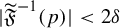 $|\widetilde {\mathfrak F}^{-1}(p)| < 2\delta $
, and if p is non-singular but lies on a singular stable leaf, then
 $|\widetilde {\mathfrak F}^{-1}(p)| < 4\delta $
.
Proof. For the moment, suppose that
 $p\in \mathcal P$
does not lie in a singular stable leaf.
Let
 $(R_i)_{i\le 0}$
be a sequence of maximal p-rectangles that limit to a horizontal leaf through p. After refining the sequence, we may assume that
 $R_{i+1}$
lies above
 $R_{i}$
for each
 $i \le -1$
. For each
 $R_i$
, let
 $\rho _i = \mathrm {ray}_p(R_i)$
be the p-ray starting at
 $R_i$
. By Proposition 6.4, each
 $\rho _i$
is contained in
 $D = D_p$
, the dynamic plane associated to p. Hence, each maximal rectangle
 $R_i$
corresponds to a vertex
 $v_i$
in D, which is the initial vertex of
 $\rho _i$
.
Next, let Q be any edge rectangle in
 $\mathcal P$
that contains p. As before, let
 $R = R_Q$
be the maximal rectangle obtained by extending Q vertically and also let
 $R'$
be the maximal rectangle obtained by extending Q horizontally. These correspond to sectors
 $\sigma = \sigma (R)$
and
 $\sigma ' = \sigma (R')$
in D, where
 $\sigma $
lies directly above
 $\sigma '$
. Indeed,
 $\sigma $
is the sector of D whose top vertex corresponds to R and similarly for
 $\sigma '$
.
By the choice of the sequence
 $(R_i)_{i\le 0}$
, the rectangle Q (and hence
 $R'$
) lies above
 $R_j$
for
 $j \ll 0$
. By Lemma 6.2, there is a dual path from
 $R_j$
to
 $R'$
, so by Lemma 3.3, we have
 $\Delta (\sigma (R_j))\subset \Delta (\sigma ') \subset D$
. Hence, we see that
 $\rho _j$
meets the descending set
 $\Delta (\sigma ')$
for all j sufficiently small. So by Lemma 6.9,
 $\rho _j$
must pass through a sector in one of the two chains for
 $\sigma $
. Since the number of such sectors is uniformly bounded by Lemma 6.8, we can pass to a subsequence so that for all
 $j \le 0$
, all
 $\rho _j$
pass through a fixed vertex
 $v_Q$
in the chain for
 $\sigma = \sigma (R_Q)$
and thereafter agree. Let
 $\rho _Q$
be the
 $\widetilde \Phi $
-ray starting at
 $v_Q$
.
Iterating this construction for a sequence of edge rectangles
 $Q_{-1}, Q_{-2}, Q_{-3},\ldots $
limiting to the horizontal leaf through p yields a nested sequence of rays
 $\rho _{Q_{-1}}\subset \rho _{Q_{-2}}\subset \rho _{Q_{-3}}\subset \ldots $
, the union of which is a
 $\widetilde \Phi $
-line
 $\ell $
in D such that each maximal rectangle along
 $\ell $
contains p. Hence,
 $\widetilde {\mathfrak F}(l) = p$
, as required.
For the bound on the preimage, note that any line in
 $\mathfrak F^{-1}(p)$
is contained in the dynamic plane
 $D_p$
for p by Proposition 6.4. Since the length of a chain of sectors is less than
 $\delta $
by Lemma 6.8, the argument above implies that there are less than
 $2 \delta \ p$
-lines in
 $D_p$
.
Next, suppose that
 $p\in \mathcal {P}$
lies on a singular stable leaf
 $\ell $
but is non-singular. Since any line in
 $\widetilde {\Phi }$
that determines a sequence of maximal rectangles containing p must eventually have p appearing in the vertical boundary of each of its rectangles, we observe that any line in the preimage
 $\mathfrak F^{-1}(p)$
is contained in one of the two dynamic planes containing
 $D_{\ell }$
introduced in Remark 6.5. Applying the same argument as in the previous case, but in each of these planes containing
 $D_{\ell }$
, produces at least two and less than
 $4\delta \ \widetilde \Phi $
-lines mapping to p under
 $\widetilde {\mathfrak F}$
.
Finally, suppose that
 $p\in \mathcal P$
is a singular point. Pick a singular stable leaf
 $\ell $
through p that is stabilized by some
 $g \ne 1$
. Then g stabilizes
 $D_{\ell }$
and we let D be one of the two dynamic planes containing
 $D_{\ell }$
, as in Remark 6.5. Since D is also stabilized by g, D contains a g-periodic line l in
 $\widetilde \Phi $
by the proof of Proposition 3.15. Since the sequence of maximal rectangles associated to l is g-invariant, the intersection of these rectangles
 $\widetilde {\mathfrak F}(l)$
contains the fixed point of g, which is the singularity p. This completes the proof.
6.3 Cycles of
$\Phi $
and closed orbits of
$\varphi $


We next define the map
 ${\mathfrak F}$
from Theorem 6.1. Let c be a directed cycle in
 $\Phi $
, let
 $\widetilde c$
be a lift of c to
 $\widetilde \Phi $
, and let
 $g \in \pi _1 (M)$
be the deck transformation that generates the stabilizer of
 $\widetilde c$
and translates in the positive direction. Then
 $ g \cdot \widetilde {\mathfrak F}(\widetilde c)=\widetilde {\mathfrak F}(g \cdot \widetilde c)=\widetilde {\mathfrak F}(\widetilde c)$
, so
 $p =\widetilde {\mathfrak F}(\widetilde c)\in \mathcal {P}$
is fixed by the action of g. Hence, p corresponds to either a g-invariant flow line
 $\widetilde \gamma $
of
 $\widetilde M$
or a singularity of
 $\mathcal P$
fixed by g. In the case where p is non-singular, the directed cycle c is homotopic in M to the closed orbit
 $\gamma = \widetilde \gamma / \langle g \rangle $
of
 $\varphi $
and we set
 $\mathfrak F(c) = \gamma $
.
When
 $p = \widetilde {\mathfrak F}(\widetilde c)$
is a singularity, each rectangle in the g-periodic sequence of maximal rectangles along
 $\widetilde c$
contains the singularity p in its vertical boundary. Indeed, p must eventually be in a vertical side of the associated rectangles (by the description of
 $\widetilde \Phi $
in terms of maximal rectangles) and so by g-periodicity, p must be in a vertical side of every maximal rectangle associated to
 $\widetilde c$
. Let
 $\ell ^u$
be the unique leaf of the unstable foliation
 $\mathcal F^u$
containing p that meets all the maximal rectangles along
 $\widetilde c$
. Then
 $\ell ^u$
is invariant under g. Let
 $\gamma $
be the unique multiple of the unstable prong curve in M determined by
 $\ell ^u$
to which c is homotopic, and set
 $\mathfrak F(c) = \gamma $
.
Recall that
 $\mathcal O_{\varphi }^+ \subset M$
is the union of closed orbits
 $\mathcal O_{\varphi }$
of the flow along with all positive multiples of unstable prong curves in M. If we denote by
 $\mathcal {Z}_{\Phi }$
the set of directed cycles of
 $\Phi $
, then the above discussion produces a map:
 $$\begin{align*}{\mathfrak F} : \mathcal{Z}_{\Phi} \to \mathcal O_{\varphi}^+, \end{align*}$$
with the property that the directed cycle c is homotopic to
 ${\mathfrak F}(c)$
in M. We remark that when
 ${\mathfrak F}(c)$
is non-singular (i.e. a closed orbit in M; not a prong curve), it is the unique closed orbit of
 $\varphi $
homotopic to the flow cycle c since the flow does not have distinct homotopic orbits.
We need to further discuss the case when
 $\widetilde {\mathfrak F}(\widetilde c)=p$
is a singularity, or equivalently when
 $\mathfrak F(c)=\gamma $
is an unstable prong curve. Let
 $\widetilde \gamma $
be the corresponding lift of
 $\gamma $
to
 $\widetilde M$
, and let U be the component of
 $\widetilde M-\widetilde B^s$
containing
 $\widetilde \gamma $
. Let T be the boundary of a small regular neighborhood of the singular orbit corresponding to
 $\gamma $
, and let
 $\widetilde T$
be the lift to
 $\widetilde M$
of T that is contained in U. We describe some structure of U and
 $\partial U$
that follows from the discussion in [Reference Landry, Minsky and TaylorLMT20, §5].
The boundary tessellation by
 $\widetilde \tau $
of
 $\widetilde T$
can be naturally identified with the tessellation
 $\partial U\cap \widetilde \tau ^{(2)}$
, because
 $\widetilde \tau ^{(2)}\cap U$
is homeomorphic to the product of the tessellation of the cusp with
 $(0,1)$
[Reference Landry, Minsky and TaylorLMT20, Lemma 5.2]. Thus it makes sense to speak of upward/downward triangles and ladders on
 $\partial U$
(see [Reference Landry, Minsky and TaylorLMT20, §2.1.2] for terminology) and the following facts are contained in Lemmas 5.3–5.5 of [Reference Landry, Minsky and TaylorLMT20]. Each upward ladder of
 $\partial U$
contains a unique branch line in its interior. The complementary components of these branch lines are called bands. Each band B contains a unique downward ladder L in its interior, and any
 $\widetilde \Phi $
-line contained in a given band must lie in L. The structure of
 $\widetilde \Phi \cap B$
is such that there is at least one and no more than two asymptotic classes of
 $\widetilde \Phi $
-lines contained in L. Further, if
 $\lambda ^u$
is the unstable leaf of
 $\widetilde \varphi $
corresponding to
 $\widetilde \gamma $
, with projection
 $\ell ^u$
in
 $\mathcal {P}$
, then the idea of the proof of [Reference LandryLan19, Lemma 2.8] shows that
 $\lambda ^u$
intersects
 $\widetilde T$
in the core of the ladder on
 $\widetilde T$
corresponding to L, and that L can be characterized as the intersection with
 $\widetilde B^s$
of all tetrahedra t such that the maximal rectangle corresponding to t intersects
 $\ell ^u$
in its interior and contains p in its boundary. It follows that
 $\widetilde c$
lies in the core of L.
This discussion gives us the following lemma.
Lemma 6.13. Let c be a
 $\Phi $
-cycle and
 $\gamma $
a prong curve such that
 $\mathfrak F(c)=\gamma $
. Then c lies in the unique band of
 $B^s$
corresponding to the downward ladder determined by
 $\gamma $
. It follows that c is transversely homotopic to
 $\gamma $
and that there are at most two
 $\Phi $
-cycles mapping to c under
 $\mathfrak F$
.
The next proposition establishes that all but finitely many primitive closed orbits of
 $\varphi $
are homotopic to directed cycles of
 $\Phi $
. Note that if the closed orbit
 $\gamma $
is homotopic to the flow cycle c, then we necessarily have
 $\mathfrak F(c) =\gamma $
since no two closed orbits of the flow are homotopic.
Proposition 6.14. Let
 $\gamma $
be a non-singular closed orbit of
 $\varphi $
. Then
 $\gamma $
is homotopic in M to either a directed cycle of the flow graph
 $\Phi $
or an odd
 $AB$
-cycle in
 $\Gamma $
.
Proof. The closed orbit
 $\gamma $
is homotopic to a (non-unique)
 $\Gamma $
-cycle c. This follows from the fact that all orbits of
 $\varphi $
are positive transverse to
 $\tau ^{(2)}$
and by perturbing
 $\gamma $
slightly, if necessary, we can assume that it misses
 $\tau ^{(1)}$
. The sequence of faces of
 $\tau $
intersected by
 $\gamma $
defines a dual cycle c homotopic to
 $\gamma $
. The proposition now follows from Proposition 3.15.
We are now ready to prove the main theorem of this section.
Proof of Theorem 6.1
For item
 $(1)$
, the definition of
 $\mathfrak F$
ensures that
 $\gamma = \mathfrak F(c)$
is homotopic to c in M. It remains to prove that c and
 $\gamma $
are transversely homotopic. When
 $\gamma $
is a regular orbit, this follows immediately from Proposition 6.7. For this, we use that the regular orbit
 $\gamma $
is not homotopic to a branch curve because branch curves in
 $\overline M$
are homotopic to singular orbits and no distinct closed orbits in
 $\overline M$
are homotopic (Lemma 4.2).
If
 $\gamma $
is instead an unstable prong curve,
 $\gamma $
is homotopic to branch curves corresponding to the same singular orbit and so Proposition 6.7 does not apply. Instead, we simply apply Lemma 6.13.
Item (2) is also a direct application of Lemma 6.13.
Item
 $(3)$
essentially follows from Lemma 6.6. For this, let
 $c_1, \ldots , c_n \in \mathcal Z_{\varphi }$
with
 $\mathfrak F(c_i) =\gamma $
. Let
 $\widetilde \gamma $
be a fixed lift of
 $\gamma $
, let
 $g \in \pi _1(M)$
generate the stabilizer of
 $\widetilde \gamma $
, and let p be the image of
 $\widetilde \gamma $
in
 $\mathcal P$
. Since each
 $c_i$
is homotopic to
 $\gamma $
, we can choose lifts
 $\widetilde c_i$
that are also invariant under g. Hence,
 $p = \widetilde {\mathfrak F}(\widetilde c_i)$
. That is, each
 $\widetilde c_i$
is a p-line in
 $\widetilde \Phi $
. By Proposition 6.4, each
 $\widetilde c_i$
is contained in the dynamic plane
 $D_p$
, and by Lemma 6.6, the number of asymptotic classes of the
 $\widetilde c_i$
is equal to the width of D. However, if two g-invariant p-lines are asymptotic, then they are equal. We conclude that n is equal to the width of
 $D_p$
. By Proposition 3.10, the width of
 $D_p$
is equal to one, unless
 $\gamma $
is homotopic to an
 $AB$
-cycle. Regardless, the width is no more than
 $\delta $
by Corollary 3.13.
Finally, item
 $(4)$
follows from Proposition 6.14 and the fact that no distinct closed orbits of
 $\varphi $
are homotopic.
Next we mention a corollary that further connects the flow and triangulation. Recall from §2.4 that
 $\mathrm {cone}_1(\Gamma ) \subset H_1(M; \mathbb {R})$
denotes the cone of homology directions of
 $\tau $
, which is the cone positively spanned by the classes of closed curves positively transverse to
 $\tau ^{(2)}$
. We proved in [Reference Landry, Minsky and TaylorLMT20, Theorem 5.1] that this agrees with the cone positively spanned by
 $\Phi $
-cycles (cf. Proposition 3.15). In [Reference FriedFri82b], Fried associates to any flow a cone of homology directions in first homology which can be thought of as the positive span of classes of nearly closed orbits. In the current context, the cone of homology directions of our pseudo-Anosov flow
 $\varphi $
is polyhedral and positively spanned by closed orbits of
 $\varphi $
. Since the flow is positively transverse to
 $\tau ^{(2)}$
away from the singular orbits, and each singular orbit has a multiple which is homotopic to a transversal by Theorem 6.1, it is clear that
 $\mathrm {cone}_1(\Gamma )$
contains Fried’s cone. Theorem 6.1 also easily implies the reverse containment, giving us the following.
Corollary 6.15. (Homology directions)
Suppose that the veering triangulation
 $\tau $
is associated to the flow
 $\varphi $
. Then the image of
 $\mathrm {cone}_1(\Gamma )$
in
 $H_1(\overline M;\mathbb {R})$
is equal to Fried’s cone of homology directions for
 $\varphi $
.
We conclude this subsection by showing that the veering triangulation also detects which orbits of
 $\varphi $
are twisted.
Lemma 6.16. Let
 $\gamma $
be a non-singular closed orbit of
 $\varphi $
and let c be any directed cycle of
 $\Gamma $
homotopic to
 $\gamma $
. Then
 $\gamma $
is untwisted if and only if c has an even number of
 $AB$
-turns.
Proof. As in the proof of Lemma 3.14, c has an even number of AB turns if and only if the pullback of the tangent bundle over
 $B^s$
is orientable [Reference Landry, Minsky and TaylorLMT20, Lemma 5.6]. Lifting to the universal cover
 $\widetilde M$
, this is equivalent to a fixed coorientation on
 $\widetilde B^s$
being preserved by the deck transformation
 $g \in \pi _1(M)$
with
 $\langle g \rangle = \mathrm {stab}(\widetilde c)$
. (We recall that since M deformation retracts to
 $B^s$
, the branched surface
 $\widetilde B^s$
is contractable. Hence, its tangent plane bundle is trivial.) Such a coorientation on
 $\widetilde B^s$
orients all edges of the lifted triangulation
 $\widetilde \tau $
and these orientations are preserved by g. Note that by looking at the intersection of
 $\widetilde B^s$
with any face of
 $\widetilde \tau $
, we see that the widest edge of the face is oriented consistently with respect to the other edges, i.e. the widest edge is the homological sum of the other two.
Now each vertex crossed by
 $\widetilde c$
corresponds to a tetrahedron of
 $\widetilde \tau $
and hence to a maximal rectangle in
 $\mathcal P$
. As in the construction of the map
 $\widetilde {\mathfrak F}$
, the intersection of all these maximal rectangles is the fixed point p of g, which by construction is the projected image of the g-periodic flow line
 $\widetilde \gamma $
. Moreover, for any positive ray
 $\widetilde c^+$
of
 $\widetilde c$
, the intersection of the associated maximal rectangles is a segment of the stable leaf
 $\ell $
through p in
 $\mathcal P$
(see Fact 4.4). The fact that the edges of
 $\tau $
are coherently oriented along the faces crossed by
 $\widetilde c$
translates to the fact that the
 $\tau $
-edges of the maximal rectangles in our collection coherently cross
 $\ell $
from one (say the left) side to the other. Since this ordering is preserved by g, the stable leaf
 $\ell $
has a g-invariant coorientation. Hence, the stable leaf through
 $\widetilde {\mathfrak F}(\widetilde \gamma )$
also has a coorientation preserved by g and so the orbit
 $\gamma $
is untwisted.
Reversing the logic, if
 $\ell $
has a g-invariant coorientation, then we can used this to coherently orient the
 $\tau $
-edges crossing
 $\ell $
and this translates to a coherent orientation on the edges of
 $\widetilde \tau $
that is compatible on faces in the above sense and which is g-invariant. Hence, the orientation on any one of these edges coorients
 $\widetilde B^s$
in a g-invariant fashion. This implies, again as in Lemma 3.14, that c has an even number of
 $AB$
-turns. The proof is complete.
7 Growth rates of orbits and the veering polynomial
In this section, we show how a modified version of the veering polynomial can detect growth rates of closed orbits of subsets of the flow, even in the non-layered setting. Our main theorems are Theorem 7.1, which relates growth rates of the flow to those of the flow graph, and Theorem 7.2, which relates the growth rates to the veering polynomial. These are new even in the case of surfaces contained in the boundary of a fibered face and more on this special case is discussed in §9.2. In Proposition 7.7, we will use these to give a topological criterion for these growth rates to be strictly greater than 1.
In §8, we extend these results to study growth rates for the closed manifold
 $\overline M$
after cutting along a transverse surface.
Cutting along a surface. Let
 $S\subset M$
be a properly embedded surface positively transverse to the flow
 $\varphi $
, and let
 $M|S$
denote M cut along S, with its components indicated as
 $M|S = \bigcup _i M|_iS$
. We let
 $\varphi |S$
denote the restricted semiflow on
 $M|S$
and let
 $\varphi |_iS$
denote the further restriction to the component
 $M_i|S$
. Let
 $\mathcal O|S$
and
 $\mathcal O|_i S$
denote the directed closed orbits of
 $\varphi |S$
and
 $\varphi |_iS$
, respectively. In particular,
 $\mathcal O|_i S$
are the closed orbits of
 $\varphi $
that are contained in
 $M|_iS$
.
Let
 $\Phi $
be the flow graph of the veering triangulation
 $\tau $
and
 $\iota : \Phi \to M$
be its embedding in dual position. If S is carried by the veering triangulation
 $\tau $
, then it is positively transverse to
 $\iota (\Phi )$
as well as the flow (Theorem 5.1), and we denote by
 $\Phi \smallsetminus S$
the flow graph cut along
 $\iota ^{-1}(S)$
. Then let
 $\Phi |S$
denote the recurrent subgraph of
 $\Phi \smallsetminus S$
, that is, the union of edges traversed by directed cycles of
 $\Phi \smallsetminus S$
. As for
 $\varphi $
, let
 $\Phi |_i S$
denote the subgraph of
 $\Phi |S$
contained in
 $M|_i S$
, and let
 ${\mathcal Z}_{\Phi |S}$
and
 ${\mathcal Z}_{\Phi |_iS}$
denote the directed cycles of
 $\Phi |S$
and
 $\Phi |_i S$
, respectively.
Now let
 $\xi \in H^1(M|_iS)$
be a cohomology class which is positive on the closed orbits
 $\mathcal O|S_i \subset M|_iS$
as well as on unstable prong curves that are contained in
 $M|S_i$
. We call any such class positive with respect to
 $\varphi |_iS$
and note that such positive classes determine a (possibly empty) open cone in
 $H^1(M|_iS)$
.
We then consider for a positive class
 $\xi $
, the exponential growth rates
 $$ \begin{align} \mathrm{gr}_{\varphi|_iS}(\xi) = \lim_{L\to \infty} \# \{ \gamma \in \mathcal O|_iS : \xi(\gamma) \le L \} ^{{1}/{L}} \end{align} $$
and
 $$ \begin{align} \mathrm{gr}_{\Phi|_iS}(\xi) = \lim_{L\to \infty} \# \{ c \in {\mathcal Z}_{\Phi|_iS} : \xi(\iota(c)) \le L \} ^{{1}/{L}}. \end{align} $$
The first main theorem of this section is the following.
Theorem 7.1. (Growth rates in
$M|_iS$
)

Let
 $\tau $
be a veering triangulation of M with dual flow
 $\varphi $
. Consider a surface S carried by
 $\tau ^{(2)}$
and fix a component
 $M|_iS$
of
 $M|S$
.
For any positive class
 $\xi \in H^1(M|_iS)$
, the growth rates of
 $\varphi |_iS$
and
 $\Phi |_iS$
exist and
 $$ \begin{align*} \mathrm{gr}_{\varphi|_iS}(\xi) = \mathrm{gr}_{\Phi|_iS}(\xi). \end{align*} $$
In fact,
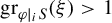 $\mathrm {gr}_{\varphi |_iS}(\xi )>1$
so long as
 $\mathcal O|_iS$
contains infinitely many primitive orbits. See Proposition 7.7.
To compute these growth rates, we will define a veering polynomial
 $V_{\varphi |_iS} \in \mathbb {Z}[H_1(M|_iS) / \text {torsion}]$
(see §7.4) directly from the Perron polynomial
 $P_{\Phi }$
of the flow graph
 $\Phi $
and obtain this theorem.
Theorem 7.2. (Growth rates and the polynomial)
Let
 $\tau $
be a veering triangulation of M with dual flow
 $\varphi $
. Consider a surface S carried by
 $\tau ^{(2)}$
and fix a component
 $M|_iS$
of
 $M|S$
.
For any positive
 $\xi \in H^1(M|_iS)$
, the growth rate
 $\mathrm {gr}_{\varphi |_i S}(\xi )$
is equal to the reciprocal of the smallest positive root of
 $V_{\varphi |_iS} ^{\xi }$
, the veering polynomial of
 $M|_iS$
specialized at
 $\xi $
.
7.1 Cutting with cohomology
We first observe that
 $\Phi |S$
depends only on the Poincaré dual of
 $[S]$
in
 $H^1(M)$
.
Lemma 7.3. The directed cycles of
 $\Phi |S$
are exactly the directed cycles of
 $\Phi $
that are zero under
 $\iota ^*\eta $
, where
 $\eta \in H^1(M)$
is the Poincaré dual of S.
Proof. Let c be a directed cycle of
 $\Phi $
. If c is in
 $\Phi |S$
, it misses
 $\iota ^{-1}(S)$
, so
 $\eta (\iota (c)) = 0$
. Conversely, if
 $\eta (\iota (c)) = 0$
, then
 $\iota (c)$
must miss S since all intersections of
 $\iota (\Phi )$
with
 $\tau ^{(2)}$
are transverse and positive.
Motivated by this, for
 $\eta \in \mathrm {cone}_2(\tau )$
, define
 $\Phi |\eta $
to be the subgraph of
 $\Phi $
whose edges are traversed by directed cycles that are
 $\iota ^*\eta $
-null. Alternatively,
 $\Phi |\eta $
is the largest recurrent subgraph of
 $\Phi $
on which the pullback of
 $\eta $
is
 $0$
(see e.g. [Reference Landry, Minsky and TaylorLMT20, Lemma 5.10]). We call
 $\Phi |\eta $
the restricted flow graph for
 $\eta $
. When
 $\eta $
is dual to a carried surface S, Lemma 7.3 implies that
 $\Phi |\eta = \Phi |S$
. Although this will not play a direct role here, we reconsider this perspective in §9.2.
7.2 Parameterizing orbits of
$\varphi |_iS$

Recall that
 $\mathcal O^+$
denotes the union of closed orbits of
 $\varphi $
,
 $\mathcal O = \mathcal O_{\varphi }$
, together with all positive multiples of the finitely many unstable prong curves of M, and we define
 $\mathcal O^+|S$
accordingly. We have
 $\mathcal O^+|S = \bigcup _i \mathcal O^+|_iS$
, where
 $\mathcal O^+|_iS$
are the closed orbits and unstable prong curves that are contained in
 $M|_iS$
.
Lemma 7.4. (Decomposing orbits)
The map
 $\mathfrak F : {\mathcal Z}_{\Phi } \to \mathcal O^+$
from Theorem 6.1 restricts to a map
 $$ \begin{align*} \mathfrak F|_iS : {{\mathcal Z}}_{\Phi |_iS} \to \mathcal O^+|_iS, \end{align*} $$
whose image is
 $\mathrm {im}({\mathfrak F}) \bigcap \mathcal O^+|_iS$
for each component
 $M|_iS$
of
 $M|S$
.
Moreover, for each directed cycle c of
 $\Phi |_iS$
,
 $\iota (c)$
is homotopic to
 $\mathfrak F(c)$
within
 $M|_iS$
.
Proof. Fix a component
 $M|_iS$
and let
 $c \in {{\mathcal Z}}_{\Phi |_iS}$
be a directed cycle of
 ${\Phi |_iS}$
. Recall from Theorem 6.1 that
 $\gamma = {\mathfrak F}(c)$
is the closed orbit or unstable prong curve of
 $\varphi $
that is transversely homotopic to
 $\iota (c)$
. That is, there is a homotopy from
 $\iota (c)$
to
 $\gamma $
through curves that are positively transverse to
 $\tau ^{(2)}$
. Since S is carried by
 $\tau $
, the curves in this homotopy are also positively transverse to, and hence disjoint from, S. Since
 $\iota (c) \subset M|_iS$
by definition of
 ${\Phi |_iS}$
, we conclude that
 $\iota (c)$
is homotopic to
 $\gamma $
within
 $M|_iS$
and so, in particular,
 $\gamma = {\mathfrak F(c)} \in \mathcal O^+|_iS$
.
Similarly, if
 $\gamma \in \mathcal O^+|_i S$
is in the image of
 ${\mathfrak F}$
, then any preimage c must be
 $0$
under
 $\iota ^*\eta $
(where
 $\eta $
is the Poincareé dual of S, as in Lemma 7.3), and hence c is in
 $\Phi |S$
. Just as above, we may additionally conclude that
 $c \in {{\mathcal Z}}_{\Phi |_iS}$
.
7.3 Comparing growth rates
We are now ready to prove Theorem 7.1. Let
 $\xi \in H^1(M|_i S)$
be positive with respect to
 $\varphi |_iS$
. By definition,
 $\xi $
is positive on
 $\mathcal O^+|_iS$
, the set of closed orbits and unstable prong curves that are contained in
 $M|_iS$
.
Lemma 7.5. If
 $\xi \in H^1(M|_i S)$
is positive, then its pullback
 $\iota ^*\xi $
to
 $H^1(\Phi |_iS)$
is positive on directed cycles.
Proof. By Lemma 7.3, for each directed cycle c of
 $\Phi |_iS$
, the image
 $\iota (c)$
is homotopic in
 $M|S_i$
to a closed orbit or unstable prong curve in
 $M|S_i$
. The lemma follows.
We shall now prove that the growth rates, counting with respect to
 $\xi $
, of closed orbits of
 $\varphi |_i S$
and directed cycles of
 $\Phi |_i S$
exist and are equal:
 $$ \begin{align*} \mathrm{gr}_{\varphi|_iS}(\xi) = \mathrm{gr}_{\Phi|_iS}(\xi). \end{align*} $$
We will use results from the theory of growth rates of cycles in directed graphs and refer to McMullen’s paper [Reference McMullenMcM15].
Proof of Theorem 7.1
Since
 $\iota ^*\xi $
is positive on directed cycles of
 $\Phi |_iS$
(Lemma 7.5), it follows that
 $\mathrm {gr}_{\Phi |_iS}(\xi )$
exists (see e.g. [Reference McMullenMcM15, Lemma 3.1]).
We first show that
 $$ \begin{align*}\mathrm{gr}_{\Phi|_iS}(\xi) \le \liminf_{L\to \infty} \# \{ \gamma \in \mathcal O|_iS : \xi(\gamma) \le L \} ^{{1}/{L}}. \end{align*} $$
For this, it suffices to assume that
 $\mathrm {gr}_{\Phi |_iS}(\xi )> 1$
, otherwise there is nothing to show. By Theorem 6.1, there is a constant m such that for any
 $\gamma \in \mathcal O^+$
,
 $\# \mathfrak F^{-1}(\gamma ) \le m$
. By Lemma 7.4,
 $\mathfrak F$
maps
 ${\mathcal Z}_{\Phi |_iS}$
into
 $\mathcal O^+|_iS$
and for each directed cycle c of
 $\Phi |_iS$
,
 $\mathfrak F(c)$
is homotopic to
 $\iota (c)$
within
 $M|_iS$
. From these facts, we have
 $$ \begin{align*} \#\{ \mathfrak F(c) \in \mathcal O|_i S: \xi(\mathfrak F(c))\le L\} &\le \#\{ c \in {\mathcal Z}_{\Phi|_i S}: \iota^*\xi(c)\le L\}\\ &\le m \cdot \#\{ \mathfrak F(c) \in \mathcal O|_i S: \xi(\mathfrak F(c))\le L\}. \end{align*} $$
Thus, we have equality of growth rates:
 $$ \begin{align*} \mathrm{gr}_{\Phi|_iS}(\xi) & = \lim_{L\to \infty} \# \{ {\mathfrak F} (c) : \xi({\mathfrak F}(c)) \le L \} ^{{1}/{L}}, \end{align*} $$
which shows, in particular, that
 $\# \{ {\mathfrak F} (c) : \xi ({\mathfrak F}(c)) \le L \}$
has exponential growth. However, the multiples of unstable prong curves in
 $\mathcal O^+|_iS$
have at most linear growth so removing them from our count does not affect the growth rate. Hence,
 $$ \begin{align} \mathrm{gr}_{\Phi|_iS}(\xi) &= \lim_{L\to \infty} \# \{ \gamma \in \mathrm{Im}(\mathfrak F) \cap \mathcal O|_iS: \xi(\gamma) \le L \} ^{{1}/{L}}\\ &\le \liminf_{L\to \infty} \# \{ \gamma \in \mathcal O|_iS: \xi(\gamma) \le L \} ^{{1}/{L}} \nonumber. \end{align} $$
For the other direction, again note that we can assume that
 $$ \begin{align*} 1< \limsup_{L\to \infty} \# \{ \gamma \in \mathcal O|_iS : \xi(\gamma) \le L \} ^{{1}/{L}}, \end{align*} $$
otherwise we are done. Hence,
 $ \# \{ \gamma \in \mathcal O|_iS: \xi (\gamma ) \le L \}$
grows exponentially. By Theorem 6.1, every primitive
 $\gamma \in \mathcal O|_iS$
is in the image of
 $\mathfrak F$
with at most finitely many exceptions corresponding to closed orbits homotopic to odd
 $AB$
-cycles. Hence, the image of
 $\mathfrak {F}|_iS$
misses at most finitely many primitive orbits in
 $\mathcal O_i|S$
and their multiples. It then follows easily that
 $$ \begin{align*} \limsup_{L\to \infty} \# \{ \gamma \in {\mathcal O}|_iS: \xi(\gamma) \le L \} ^{{1}/{L}} \le \mathrm{gr}_{\Phi|_iS}(\xi), \end{align*} $$
and the proof is complete.
7.4 Adapting the veering polynomial and counting orbits
The last object needed for our discussion is an adapted version of the veering polynomial. For the directed graph
 $\Phi |S = \bigcup _i \Phi |_iS$
, let
 $P_{\Phi |S}$
and
 $P_{\Phi |_iS}$
denote the respective Perron polynomial. For each component
 $M|_iS$
of
 $M|S$
, define its veering polynomial to be
 $$ \begin{align*} V_{\varphi|_iS} = \iota_*(P_{\Phi|_iS}) \in \mathbb{Z}[H_1(M|_iS)/\text{torsion}], \end{align*} $$
where
 $\iota _* : \mathbb {Z}[H_1(\Phi |_iS)] \to \mathbb {Z}[H_1(M|_iS)/\text {torsion}]$
is the ring homomorphism induced by inclusion.
It not hard to see that
 $$ \begin{align*} P_{\Phi|S} = \prod_i P_{\Phi|_iS} \end{align*} $$
in
 $ \mathbb {Z}[H_1(\Phi |S)] = \bigotimes _i \mathbb {Z}[H_1(\Phi |_iS)]$
since
 $\Phi |S$
is the disjoint union of the
 $\Phi |_iS$
. Indeed, in this case, the adjacency matrix for
 $\Phi |S$
is a block diagonal matrix whose blocks are the adjacency matrices for the
 $\Phi |_iS$
.
Recall from §2.3 that any directed graph D has a cycle complex
 $\mathcal {C}(D)$
whose cliques are the disjoint simple directed cycles of D. Moreover, the Perron polynomial
 $P_D$
of D is equal to the clique polynomial of
 $\mathcal {C}(D)$
.
Proposition 7.6. Let
 $\eta \in H^1(M)$
be the Poincaré dual to S. The inclusion
 $\Phi |S\to \Phi $
induces an inclusion
 $\mathcal {C}(\Phi |S) \to \mathcal {C}(\Phi )$
whose image is the full subcomplex spanned by simple cycles that are zero under
 $\iota ^*\eta $
.
Hence,
 $P_{\Phi |S}$
can be obtained from
 $P_{\Phi }$
by removing terms which evaluate non-trivially under
 $\eta $
.
Proof. Since
 $\Phi |S \to \Phi $
is inclusion, we have the inclusion of vertices
 $\mathcal {C}^0(\Phi |S) \to \mathcal {C}^0(\Phi )$
. This amounts to saying that simple cycles of
 $\Phi |S$
map to simple cycles of
 $\Phi $
. The full inclusion statement is then equivalent to saying that cycles
 $c_1$
and
 $c_2$
of
 $\Phi |S$
are disjoint if and only if they are disjoint as cycles in
 $\Phi $
. This is equally clear.
Finally, as in §2.3, we know that the Perron polynomial
 $P_{\Phi }$
is equal to
 $$ \begin{align*} 1 + \sum_{\sigma} -1^{|\sigma|} \sigma, \end{align*} $$
where the sum is over cliques of
 $\mathcal {C}(\Phi )$
. Hence, the only terms of
 $P_{\Phi }$
that do not appear in
 $P_{\Phi |S}$
are those composed of multicurves that have positive evaluation under
 $\iota ^*\eta $
. This completes the proof.
We henceforth consider
 $P_{\Phi |S}$
as being obtained from
 $P_{\Phi }$
by removing the terms that correspond to cycles which are non-trivial under
 $\iota ^*\eta $
.
We can now prove Theorem 7.2 which relates growth rates of
 $\varphi $
in
 $M|_iS$
to the veering polynomial.
Proof of Theorem 7.2
Let
 $\iota : \Phi |_iS \to M|_iS$
be as above. Since
 $\xi $
is positive,
 $\iota ^*\xi $
is positive on all directed cycles of
 $\Phi |_iS$
(Lemma 7.5).
By [Reference McMullenMcM15, Theorem 3.2],
 $\mathrm {gr}_{\Phi |_iS}(\xi ) $
is equal to the reciprocal of the smallest root of the Perron polynomial of
 $P_{\Phi |_iS}$
specialized at
 $\iota ^*\xi $
. (Technically, this is applied to a metric on
 $\Phi |_i S$
representing
 $\iota ^*\xi $
; see [Reference McMullenMcM15, Lemma 5.1] or [Reference Landry, Minsky and TaylorLMT20, Lemma 5.10].) Since
 $$ \begin{align*} P_{\Phi|_iS}^{\iota^*\xi} = V_{\varphi|_iS}^{\xi}, \end{align*} $$
the result follows from Theorem 7.1.
We conclude this section with a characterization of when the entropy is positive.
Proposition 7.7. With notation as in Theorem 7.1, the growth rate
 $\mathrm {gr}_{\varphi |_iS}(\xi )$
is strictly greater than
 $1$
for every positive
 $\xi \in H^1(M|_iS)$
if and only if there are infinitely many primitive closed orbits of
 $\varphi $
contained in
 $M|_iS$
.
Proof. If
 $\mathrm {gr}_{\varphi |_iS}(\xi )>1$
, then the claim that there are infinitely many primitive closed orbits in
 $M|_iS$
is clear, since otherwise the growth of all orbits is linear.
Now suppose that there are infinitely many primitive closed orbits in
 $M|_iS$
. Then, as in the proof of Theorem 7.1, there are infinitely many closed primitive cycles in
 $\Phi |_iS$
. Since the directed graph
 $\Phi |_iS$
is finite, this mean that it has recurrent components that are neither trivial nor cyclic. Hence, the growth rate of directed cycles with respect to any positive cocycle is strictly greater than
 $1$
. As this quantity is the same as
 $\mathrm {gr}_{\varphi }(\xi )$
, the proof is complete.
8 Transverse surfaces and growth rates for closed manifolds
In this section, we outline a way in which the results of the previous section extend to closed
 $3$
-manifolds. Here, the veering triangulation is still the central tool but does not appear in theorem statements.
Let
 $\overline M$
be a closed
 $3$
-manifold and let
 $\varphi $
be a pseudo-Anosov flow on
 $\overline M$
without perfect fits. Let S be a closed surface in
 $\overline M$
that is transverse to
 $\varphi $
. For simplicity of notation, we will assume that S is connected. We orient S so that each intersection with an orbit of
 $\varphi $
is positive and note that
 $M|S$
is connected. Let
 $\mathcal O|S$
be the set of closed orbits of
 $\varphi $
that miss S and hence are contained in
 $M|S$
. Below, we will define an invariant
 $V_{\varphi |S} \in \mathbb {Z}[H_1(\overline M|S)]/\mathrm {torsion}$
which we call the veering polynomial of
 $\overline M|S$
. We will call a class
 $\xi \in H^1(\overline M|S)$
strongly positive if it is positive on
 $\mathcal O|S$
as well as a certain finite collection of curves in
 $\partial M|S$
that we define below (§8.2).
We will prove the following theorem.
Theorem 8.1. Let
 $\varphi $
be a pseudo-Anosov flow on
 $\overline M$
without perfect fits. Let S be a closed connected surface in
 $\overline M$
that is transverse to
 $\varphi $
.
For any strongly positive class
 $\xi \in H^1(\overline M|S)$
, the growth rate
 $$ \begin{align*} \mathrm{gr}_{\varphi|S}(\xi) = \lim_{L\to \infty} \# \{ \gamma \in \mathcal O|S : \xi(\gamma) \le L \} ^{{1}/{L}} \end{align*} $$
of closed orbits in
 $M|S$
exists and equals the reciprocal of the smallest root of the specialization
 $V_{\varphi |S}^{\xi }$
of the veering polynomial.
Recall that
 $M = \overline M \smallsetminus \{\text {singular orbits}\}$
admits a veering triangulation
 $\tau $
. Let
 $\iota : \Phi \to M \subset \overline M$
be the embedding of the flow graph in dual position so that its edges are positively transverse to
 $\tau ^{(2)}$
. Fix S as in the statement of Theorem 8.1 and let
 $\eta \in H^1(\overline M)$
be its Poincaré dual.
We begin by noting that if we also puncture S along the singular orbits of
 $\varphi $
, we obtain a surface
 $\mathring S$
in M that is positively transverse to the remaining orbits. However, it is not clear whether
 $\mathring S$
is necessarily carried by the branched surface
 $\tau ^{(2)}$
and so the results of the previous section do not automatically apply. Instead, we use the following claim, which is all we will need.
Claim 8.2. (Homotoping the flow graph)
Let S be a closed surface positively transverse to
 $\varphi $
. The flow graph
 $\iota : \Phi \to \overline M$
can be isotoped to a map
 $\iota _0 : \Phi \to \overline M$
so that its edges are positively transverse to S.
Proof. Since the surface S is positively transverse to
 $\varphi $
, results in [Reference MosherMos92b] imply that S is taut and so its Thurston norm equals
 $\vert \chi (S) \vert $
. Applying the Poincaré–Hopf index formula to the singular foliation
 $\mathcal F^{\kern1.3pt s} \cap S$
of S, we see that
 $\chi (S) = e_{\tau }(S)$
, where
 $e_{\tau }$
is the combinatorial Euler class of [Reference LandryLan22]. Then the main theorem of [Reference LandryLan22] states that there exists an isotopy that pushes a certain family of annuli of S into a neighborhood of the singular orbits so that outside this neighborhood, S is carried by
 $\tau ^{(2)}$
. This implies, in particular, that we may isotope the flow graph
 $\Phi $
in
 $\overline M$
to be positively transverse to S, as required.
For the proof of Theorem 8.1, we wish to follow along the lines of the proofs for Theorems 7.1 and 7.2, except that we no longer have the full strength of the veering triangulation available (see §8.2). In what follows, we adapt the argument to only use the fact that the flow graph
 $\Phi $
is positively transverse to the surface S.
As before, we define
 $\Phi \smallsetminus S$
by cutting
 $\Phi $
along
 $\iota _0^{-1}(S)$
and we take its recurrent subgraph
 $\Phi |S$
. By construction, the restriction
 $\iota _0 : \Phi |S \to \overline M|S$
is defined and
 $\Phi |S$
is exactly the subgraph of
 $\Phi $
consisting of edges that are traversed by cycles which are
 $0$
under
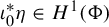 $\iota _0^*\eta \in H^1(\Phi )$
(cf. Lemma 7.3).
8.1 Stable and unstable curves
The main complication in studying flows in the cut manifold
 $\overline M|S$
is that orbits of the restricted flow may be homotopic into S itself. We begin by analyzing this possibility.
For any embedded surface S in
 $\overline M$
that is positively transverse to
 $\varphi $
, we define the singular foliations
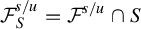 $\mathcal F_S^{s/u} = \mathcal F^{s/u} \cap S$
on S. The following is an observation that follows easily from work of Cooper–Long–Reid [Reference Cooper, Long and ReidCLR94] in the case of a circular flow and more generally from Fenley [Reference FenleyFen99b].
Lemma 8.3. Suppose that
 $\gamma $
is a closed orbit of
 $\varphi $
that is homotopic to a closed curve c in S. Then c is homotopic in S to a closed leaf of either
 $\mathcal F_S^s$
or
 $\mathcal F_S^u$
.
Moreover, every closed leaf of
 $\mathcal F_S^s$
or
 $\mathcal F_S^u$
can be oriented so that it is homotopic to a closed orbit of
 $\varphi $
.
Note that the conclusion of the lemma places c into one of at most finitely many homotopy classes of curves in S and implies that there are at most finitely many closed orbits of
 $\varphi $
that are homotopic into S. Here we are using the fact that no distinct closed orbits of
 $\varphi $
are homotopic (see Lemma 4.2(3)).
We call the closed leaves of
 $\mathcal F_S^{s/u}$
, with their orientation determined by Lemma 8.3, the stable/unstable curves of S.
Proof. Consider lifts
 $\widetilde \gamma , \widetilde c\subset \widetilde S$
to the universal cover
 $\widetilde {\overline M}$
chosen so that there is a deck transformation
 $g \in \pi _1(S)$
preserving
 $\widetilde \gamma $
,
 $\widetilde c$
and
 $\widetilde S$
. Further assume that g translates
 $\widetilde \gamma $
in its positive direction. We note that
 $\widetilde S$
is a properly embedded plane in
 $\widetilde {\overline M}$
that is positively transverse to the lifted flow. Since
 $\widetilde S$
separates
 $\widetilde {\overline M}$
, this implies that
 $\widetilde S$
intersects each flow lines at most once. Let
 $\widetilde {\mathcal F}^{s/u}(\widetilde \gamma )$
be the stable/unstable leaves through
 $\widetilde \gamma $
.
Now consider the projections to the flow space
 $\mathcal Q$
of
 $\overline M$
. To keep the notation as simple as possible, the projection of
 $\widetilde x$
in
 $\widetilde {\overline M}$
to
 $\mathcal Q$
will be denoted by
 $\widehat x$
. Since
 $\gamma $
is homotopic into S, it has intersection pairing 0 with it, which means by positive transversality of S to the flow that
 $\gamma $
misses S and hence
 $\widehat \gamma $
is not contained in
 $\widehat S$
. According to [Reference FenleyFen99b, Proposition 4.3], the boundary of
 $\widehat S$
in
 $\mathcal Q$
is a disjoint union of leaf lines, which are lines of the foliations
 $\widehat {\mathcal {F}}^{s/u}$
that are regular on their
 $\widehat S$
-side, meaning that each compact subsegment of the line is contained in the boundary of a maximal rectangle whose interior is contained in
 $\widehat S$
. (This is discussed in more detail in §9.1 where a generalization is also proven.)
Let
 $\ell $
be the unique leaf of either the stable or unstable foliation in the boundary of
 $\widehat S$
that separates
 $\widehat \gamma $
from
 $\widehat S$
. Since g stabilizes
 $\widehat \gamma $
and
 $\widehat S$
, it also stabilizes
 $\ell $
. Hence, g fixes a point in
 $\ell $
and, because fixed points are unique, we conclude that
 $\widehat \gamma \in \ell $
(Lemma 4.2). If
 $\ell $
is a leaf of the stable foliation, then the unstable leaf through
 $\widehat \gamma $
meets
 $\widehat S$
. Otherwise,
 $\ell $
is a leaf of the unstable foliation and the stable leaf through
 $\widehat \gamma $
meets
 $\widehat S$
. This means that one of the stable or unstable leaves of
 $\widetilde {\mathcal F}^{s/u}$
through
 $\widetilde \gamma $
intersects
 $\widetilde S$
in a g-invariant line. This line descends to a closed curve of
 $\mathcal F_S^{s/u}$
homotopic to c in S, and this finishes the proof in this direction.
Conversely, any closed leaf of
 $\mathcal {F}_S^{s/u}$
is contained in a leaf of
 $\mathcal {F}^{s/u}$
that is either an annulus, a Mobius band, or singular. In either case, the ‘core’ of this leaf is a closed orbit of
 $\varphi $
and the proof is complete.
8.2 Strongly positive classes in
$H^1(\overline M|S)$

In our current setting, we would like to have an analog of Lemma 7.4 stating that if c is a directed cycle in
 $\Phi |S$
and
 $\gamma \in \mathcal O|S$
is the unique orbit of
 $\varphi $
homotopic to
 $\iota _0(c)$
, then
 $\gamma $
and
 $\iota _0(c)$
are homotopic in
 $\overline M|S$
. Unfortunately, this does not seem to necessarily hold without the additional assumption that
 $S \cap M$
is carried by
 $\tau $
(see the discussion preceding Claim 8.2). We have introduced the stable/unstable curves of S, and Lemma 8.3, precisely to deal with this issue.
Now define
 $\mathcal O^{\partial }|S$
to be the set of closed orbits
 $\mathcal O|S$
together with positive multiples of the stable/unstable curves of S contained in
 $\partial (\overline M|S)$
. We call a class
 $\xi \in H^1(\overline M|S)$
strongly positive if it is positive on
 $\mathcal O^{\partial }|S$
.
Lemma 8.4. (Strong positivity)
A class
 $\xi \in H^1(\overline M|S)$
is strongly positive if and only if
 $\xi $
is positive on any oriented curve of
 $\overline M|S$
that is homotopic in
 $\overline M$
to a closed orbit of
 $\varphi $
.
Moreover, for any strongly positive
 $\xi \in H^1(\overline M|S)$
, the pullback
 ${\iota _0}^*\xi \in H^1(\Phi |S)$
is positive on directed cycles.
Proof. Let us first show that the two properties are equivalent.
By Lemma 8.3, every oriented curve in
 $\mathcal O^{\partial }|S$
is homotopic in
 $\overline M$
to a closed orbit of
 $\varphi $
. Hence, any class
 $\xi $
positive on closed orbits is positive on
 $\mathcal O^{\partial }| S$
.
Conversely, suppose that
 $\xi $
is positive on
 $\mathcal O^{\partial }|S$
and let c be an oriented curve in
 $\overline M|S$
that is homotopic in
 $\overline M$
to a closed orbit
 $\gamma $
. Then either this homotopy can be altered to live in
 $\overline M|S$
, and so
 $\xi $
is positive on c, or
 $\gamma $
is homotopic (in
 $\overline M$
) to a stable/unstable curve in the boundary of
 $\overline M|S$
(Lemma 8.3) which is homotopic in
 $\overline M|S$
to c. (To see this, note first that
 $\gamma $
cannot cut through S by positive transversality of S, and consider a homotopy from c to
 $\gamma $
that is transverse to S.) Hence,
 $\xi $
is positive on c.
That these statements imply positivity on directed cycles of
 $\Phi |S$
follows from Theorem 6.1 because for any directed cycle c of
 $\Phi |S$
,
 ${\iota _0}(c)$
is an oriented curve in
 $\overline M|S$
which is homotopic in
 $\overline M$
to a closed orbit of
 $\varphi $
.
We now turn to the proof of Theorem 8.1.
Proof of Theorem 8.1
Let
 ${\iota _0} : \Phi |S \to \overline M|S$
be as above. Since
 $\xi $
is strongly positive,
 ${\iota _0}^*\xi $
is positive on all directed cycles of
 $\Phi |S$
by Lemma 8.4. The proof is the same as for Theorem 7.2, once we establish that the growth rate
 $\mathrm {gr}_{\varphi |S}(\xi )$
exists and equals
 $$ \begin{align*} \mathrm{gr}_{\Phi|S}(\xi) = \lim_{L\to \infty} \# \{ c \in {\mathcal Z}_{\Phi|S} : \xi({\iota_0}(c)) \le L \} ^{{1}/{L}}. \end{align*} $$
For this, a slightly more delicate argument is needed since Lemma 7.4 is not available in the closed setting.
We begin by defining a map
 $\mathfrak H$
from directed cycles of
 $\Phi |S$
to
 $\mathcal O^{\partial }|S$
. To do so, we make use of the map
 $\mathfrak F : {\mathcal Z}_{\Phi } \to \mathcal O^+$
and use the basic fact that since
 $M \subset \overline M$
,
 $\mathfrak F(c)$
is homotopic to
 ${\iota _0}(c)$
in
 $\overline M$
and each unstable prong curve in M is homotopic in
 $\overline M$
to the corresponding singular orbit. Define a slight modification
 $\mathfrak F' : {\mathcal Z}_{\Phi } \to \overline {\mathcal O}$
, where
 $\overline {\mathcal O}$
is the set of all closed orbits of
 $\varphi $
in
 $\overline M$
, by setting
 $\mathfrak F'(c) = \mathfrak F(c)$
if
 $\mathfrak F(c)$
is a non-singular orbit. Otherwise,
 $\mathfrak F(c)$
is an unstable prong curve and we set
 $\mathfrak F'(c)$
to be the corresponding singular orbit.
To define
 $\mathfrak H$
, first suppose that c is a directed cycle in
 $\Phi |S$
and that
 ${\iota _0}(c)$
is homotopic to
 $\mathfrak F'(c)$
in
 $M|S$
. Then
 $\mathfrak H (c) = \mathfrak F'(c) \in \mathcal O^{\partial }|S$
. Otherwise, as in the proof of Lemma 8.4,
 ${\iota _0}(c)$
is homotopic in
 $M|S$
to some stable/unstable curve in
 $\partial (M|S)$
. We pick such a stable/unstable curve and call it
 $\mathfrak H(c)$
. Note that in either case,
 $\mathfrak H(c)$
is homotopic in
 $M|S$
to
 ${\iota _0}(c)$
.
Now the proof is completed exactly as in Theorem 7.1 by using the map
 $\mathfrak H$
and recalling that the stable/unstable curves in
 $\mathcal O|S$
have at most linear growth. To apply that argument, it only remains to show that there is some constant m such that
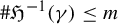 $\# \mathfrak H^{-1}(\gamma ) \le m$
for each
 $\gamma \in \mathcal O^{\partial }|S$
. Indeed, if
 $\gamma $
is a non-singular closed orbit
 $\mathfrak H$
that is interior to
 $M|S$
, then
 $\# \mathfrak H^{-1}(\gamma ) \le \# \mathfrak F^{-1}(\gamma )$
, which is bounded by Theorem 6.1. If
 $\gamma $
is a singular orbit, then there are
 $\deg (\gamma )$
unstable prong curves homotopic to
 $\gamma $
. Since each of these has at most
 $2$
preimages under
 $\mathfrak F$
, again by Theorem 6.1, we are also done in this case. Finally, suppose that
 $\gamma $
is a multiple of a stable/unstable curve of S. Note that if directed cycles c and d of
 $\Phi |S$
have
 $\mathfrak H(c) = \mathfrak H(d) = \gamma $
, then
 ${\iota _0}(c)$
and
 $i_0(d)$
are also homotopic in M. If
 $\mathfrak F(c)$
is a closed orbit, then
 $\mathfrak F(d)$
is the same closed orbit. Otherwise,
 $\mathfrak F(c)$
and
 $\mathfrak F(d)$
are homotopic unstable prong curves. In either case, we again obtain a bound on
 $\# \mathfrak H^{-1}(\gamma )$
and the proof is complete.
9 Entropy functions and stretch factors
Here we consider some applications of Theorems 7.1 and 7.2. In §9.1, we define and establish properties of the entropy function on the cone of positive cohomology classes, and in §9.2, we collect applications to the classical setting of fibered manifolds and stretch factors.
9.1 Entropy function on positive cones
Let us return to the setup of Theorem 7.1. To simplify notation, let
 $N = M|_iS$
be a fixed component of
 $M|S$
for a surface S carried by
 $\tau $
. Similarly, let
 $\Phi |N = \Phi |_iS$
be the flow graph restricted to N and note that it may have several components, each of which is strongly connected. As before, we consider N with the restricted semiflow
 $\varphi |N$
and denote by
 $\mathcal O^+|N$
its set of closed orbits and positive multiples of unstable prong curves.
Let
 ${\mathcal C}^+ \subset H^1(N; \mathbb {R})$
be the cone consisting of positive classes. According to Theorem 7.1,
 $\mathrm {gr}_{\varphi |N} : {\mathcal C}^+ \to [1,\infty )$
defines a function that gives the exponential growth rates of closed orbits of the flow for each
 $\xi \in {\mathcal C}^+$
. Since the value
 $\mathrm {gr}_{\varphi |N}(\xi )$
is given by the reciprocal of the smallest root of
 $P_{\Phi |N}$
specialized at
 $\iota ^*\xi $
by Theorem 7.2, we can use results of McMullen to study its properties.
For this, we define the associated entropy function:
 $$ \begin{align*} \mathrm{ent}_{\varphi|N} (\xi) = \log(\mathrm{gr}_{\varphi|N} (\xi)) \end{align*} $$
and note that Proposition 7.7 characterizes when entropy is non-zero. Our next theorem summarizes the entropy function’s basic properties.
Theorem 9.1. (Entropy)
The entropy function
 $\mathrm {ent}_{\varphi |N} : {\mathcal C}^+ \longrightarrow [0,\infty )$
is continuous, convex, and has degree
 $-1$
, that is,
 $\mathrm {ent}_{\varphi |N}(r \cdot \xi ) = 1/r \cdot \mathrm {ent}_{\varphi |N}(\xi )$
for
 $r>0$
.
Proof. As noted above, by Proposition 7.7, there is nothing to prove if there are only finitely many closed primitive orbits in N since then the entropy function is
 $0$
. So we assume that this is not the case. That
 $\mathrm {ent}_{\varphi |N}$
has degree
 $-1$
follows directly from the definition.
The restricted flow graph
 $\Phi |N$
is itself the disjoint union of recurrent subgraphs. For each such component J, the inclusion
 $\iota : \Phi |N \to N$
induces a pullback
 $\iota ^*: H^1(N) \to H^1(J)$
that maps the positive cone
 ${\mathcal C}^+$
to the cone
 ${\mathcal C}^+(J)$
of positive classes on J, that is, classes that are positive on directed cycles of J. Let
 $\mathrm {ent}_J : {\mathcal C}^+(J) \to [0,\infty )$
denote the corresponding entropy function. Clearly this function is 0 when J is a cycle. When it is not, since J is strongly connected, McMullen [Reference McMullenMcM15, Theorem 5.2] shows that
 $\mathrm {ent}_J$
is real-analytic, strictly convex, and blows up at the boundary of
 ${\mathcal C}^+(J)$
(that is, tends to infinity along a sequence that converges to a point in the boundary).
From Theorem 7.1, we know that on
 ${\mathcal C}^+$
, entropy is equal to the pointwise max over the components of
 $\Phi |N$
:
 $$ \begin{align} \mathrm{ent}_{\varphi|N} = \mathrm{ent}_{\Phi|N} \circ \iota^*= \max\{\mathrm{ent}_J\circ \iota^* \}, \end{align} $$
and so we immediately obtain that
 $\mathrm {ent}_{\varphi |N}$
is continuous and convex.
Remark 9.2. (Strongly positive cones for
$\overline M|S$
)

A version of Theorem 9.1 also applies to the setup of §8, where S is a closed connected transverse surface in the closed manifold
 $\overline M$
. In this case,
 ${\mathcal C}^+ \subset H^1(\overline M|S)$
is the cone of strongly positive classes as defined in §8.2.
In the special case of a fibered cone (that is, when
 $S= \emptyset $
as in §9.2) it is well known that the entropy function on the interior of the fibered cone is real analytic, strictly convex, and blows up at the boundary [Reference FriedFri82b, Reference McMullenMcM00]. However, this does not generally need to be the case for
 $\mathrm {ent}_{\varphi |N} : {\mathcal C}^+ \longrightarrow [0,\infty )$
defined here. For example, if the manifold N has a non-separating properly embedded essential annulus disjoint from all of its closed orbits, then this annulus is dual to a non-trivial cohomology class a on the boundary of
 ${\mathcal C}^+$
that pulls back to
 $0$
under
 $\iota ^*: H^1(N) \to H^1(\Phi |N)$
. If
 $u\in \mathcal {C}^+$
, then
 $\{u+ta\mid t\in [0,1]\}$
is a line segment in
 $\mathcal {C}^+$
on which
 $\mathrm {ent}_{\varphi |N}$
is constant, so
 $\mathrm {ent}_{\varphi |N}$
is not strictly convex in this case. Similarly, if N contains an essential separating annulus disjoint from the closed orbits, then
 $\mathrm {ent}_{\varphi |N}$
may not be real analytic since more than one term of the maximum in equation (9.1) may be realized.
However, more can be said if the semiflow
 $\varphi |N$
satisfies stronger dynamical conditions. To motivate the definition, first recall that, as in the proof of Lemma 4.2, the flow
 $\varphi $
is always transitive on
 $\overline M$
, meaning that it has an orbit that is dense in both the forward and backward directions. It is also well known that the closed orbits of
 $\varphi $
generate
 $H_1(\overline M; \mathbb {R})$
as a vector space. We say that the induced semiflow
 $\varphi |N$
is essentially transitive if
 $\mathcal O^+|N$
generates
 $H_1(N; \mathbb {R})$
as a vector space, and if the semiflow has an orbit that accumulates on each closed orbit of
 $\varphi |N$
in the forward direction (that is, the closure of any forward ray contains all closed orbits) and meets every neighborhood of each end of N that contains an unstable prong curve. We note that each end of N is either an annulus or torus cross an interval.
The following theorem establishes the strongest properties of
 $\mathrm {ent}_{\varphi |N}$
for essentially transitive flows.
Theorem 9.3. If the semiflow
 $\varphi |N$
is essentially transitive, and
 $\mathrm {ent}_{\varphi |N}$
is not identically 0, then
 $\mathrm {ent}_{\varphi |N}$
is real-analytic, strictly convex, and blows up at the boundary of
 ${\mathcal C}^+$
.
Before beginning the proof, we require an understanding of carried surfaces and their relation to the flow space. We define a generalized leaf
 $\ell $
of the stable/unstable foliation of
 $\mathcal P$
to be either a non-singular leaf or the union of two singular leaves at the (unique) singularity they contain. We say that a generalized stable leaf is regular to one of its sides if either it is non-singular or the singularity that it contains has exactly one singular unstable leaf meeting the interior of that side. The definition of a generalized unstable leaf that is regular to one of its sides is analogous. We note that a generalized leaf
 $\ell $
is regular to one side if and only if every finite segment of
 $\ell $
is contained in the boundary of a rectangle R; this rectangle is necessarily contained in the regular side of
 $\ell $
. We also define the boundary of an orthant at p to be the union of a singular stable leaf at p and a singular unstable leaf at p that are adjacent in the ordering around p.
Now suppose that S is a connected surface carried by
 $\tau ^{(2)}$
and hence transverse to the flow
 $\varphi $
. Consider a lift
 $\widetilde S$
of S to the universal cover
 $\widetilde M$
, and observe that
 $\widetilde S$
is a properly embedded, ideally triangulated plane in
 $\widetilde M$
(the triangulation being induced by
 $\widetilde \tau $
) that is positively transverse to the lifted flow. Since
 $\widetilde S$
separates
 $\widetilde M$
, this implies that
 $\widetilde S$
intersects each flow line at most once. Hence, the projection of
 $\widetilde S$
to the flow space
 $\mathcal P$
is a homeomorphism onto its image and we will consider its image with the projected ideal triangulation. As in §8.1, the projection of
 $\widetilde x\subset \widetilde M$
to
 $\mathcal P$
will be denoted by
 $\widehat x$
.
The following lemma generalizes [Reference Cooper, Long and ReidCLR94, Proposition 3.9] and [Reference FenleyFen99b, Proposition 4.3].
Lemma 9.4. The topological boundary of
 $\widehat S$
in
 $\mathcal P$
is a disjoint union of stable and unstable generalized leaves that are regular to their
 $\widehat S$
-side, along with boundaries of orthants and isolated singularities.
Boundaries of orthants correspond to punctures of S whose boundary slopes are those of prong curves, and isolated singularities correspond to punctures of S whose boundary slopes are not those of prong curves.
Proof. The region
 $\widehat S$
has an ideal triangulation
 $\mathcal {T}$
inherited from
 $\widetilde S$
whose vertices are singularities of
 $\mathcal P$
in the closure of
 $\widehat S$
and whose edges are singularity-free diagonals, that is,
 $\tau $
-edges. We will see that components of the boundary of
 $\widehat S$
, other than isolated singularities, are limit sets of edges of this triangulation and that these limit sets have the required form.
If x is an isolated singular point in the boundary of
 $\widehat S$
, then
 $\widetilde S$
intersects every singular leaf meeting x. It follows that the corresponding puncture of S has a slope which is not that of a prong curve.
Let x be a non-singular point in the boundary of
 $\widehat S$
and let
 $(x_i)_{i\ge 0}$
be a sequence in
 $\widehat S$
converging to x. We can assume that each
 $x_i$
lies in the interior of an edge
 $e_i$
of
 $\mathcal {T}$
and that
 $e_i,e_{i+1}$
are incident to a common face of
 $\mathcal {T}$
for each
 $i\ge 0$
. Since x is not a singularity, we may further assume that the
 $e_i$
are distinct.
Let
 $Q_i$
be the edge rectangle of
 $e_i$
. The sequence
 $(Q_i)$
cannot have both an upper bound and a lower bound with respect to the ‘above/below’ partial order on rectangles. This is due to the discreteness of singularities as in the proof of Fact 4.4. Without loss of generality, suppose that there is no rectangle R that lies above each
 $Q_i$
. In this case, we will see that
 $Q_i$
limit to a stable leaf or to a generalized stable leaf. The other case, where
 $(Q_i)$
has no lower bound, the limit is an unstable leaf or generalized leaf and is handled similarly.
First suppose that the stable leaf
 $\ell $
through x is non-singular. We will show that
 $\ell $
is in the boundary of
 $\widehat S$
. For this, let R be any maximal rectangle containing a (vertical) leaf segment of
 $\ell $
through x. For sufficiently large i,
 $x_i$
is contained in the interior of R and
 $Q_i$
does not lie below R. Since
 $Q_i$
is the edge rectangle for
 $e_i$
containing
 $x_i$
, it must be that
 $Q_i$
lies above R for large enough i. By applying the same argument to rectangles R that contain increasingly larger leaf segments of
 $\ell $
about x, and using the fact that such rectangles converge to
 $\ell $
, we see that
 $Q_i$
and hence
 $e_i$
limit to
 $\ell $
.
This shows that
 $\ell $
is in the closure of
 $\widehat S$
in
 $\mathcal P$
. To see that it is in the boundary, it suffices to show that no point of
 $\ell $
is contained in
 $\widehat S$
. This is easy since any point
 $y \in \widehat S \cap \ell $
would be contained in a face f of the triangulation
 $\mathcal {T}$
of
 $\widehat S$
which crosses
 $\ell $
. However, f would then have to be crossed by the edges
 $e_i$
for large i, which contradicts that these are all cells of a fixed triangulation
 $\mathcal {T}$
.
It remains to consider the case where the (stable) leaf through x contains a singularity p. The above argument still applies with a few minor modifications. Again, let
 $x_i, e_i, Q_i$
be defined as above and let
 $\ell $
be the stable generalized leaf through x, containing p, that is regular to its side that contains infinitely many of the
 $x_i$
. Let R be any maximal rectangle that contains a leaf segment of
 $\ell $
through x and p in its vertical boundary. If the edges
 $e_i$
do not eventually all terminate at the singularity p, then the same argument as above implies that
 $Q_i$
, and hence
 $e_i$
, limit to
 $\ell $
. So the entire generalized leaf
 $\ell $
is in the boundary of
 $\widehat S$
as required.
Otherwise, the edges
 $e_i$
eventually all have p as a singular endpoint. In this case, the rectangles
 $Q_i$
and edges
 $e_i$
limit to the singular stable leaf
 $\ell '$
through x terminating at p (that is, the half of
 $\ell $
containing x). Since the set of edges
 $e_i$
is finite up to the
 $\pi _1(S)$
action, and these edges all eventually have p as a singular endpoint, there is a
 $g \in \pi _1(S)$
fixing p and an edge e of
 $\mathcal {T}$
with endpoint p such that
 $(g^j(e))_{j\ge 0}$
occurs as a subsequence
 $(e_i)$
, and hence converges to
 $\ell '$
. This implies that g stabilizes
 $\ell '$
and hence stabilizes all stable/unstable leaves at p. However, then the sequence
 $(g^j(e))_{j \le 0}$
converges to the unstable leaf
 $\ell "$
through p such that
 $\ell ' \cup \ell "$
forms the boundary of an orthant. In this case, one easily sees that
 $g \in \pi _1(S)$
is peripheral and since it fixes each prong at p, the corresponding slope is that of a prong curve as claimed.
With Lemma 9.4 in hand, we can turn to the proof of Theorem 9.3.
Proof of Theorem 9.3
The theorem will follow fairly directly from the following claim.
Claim 9.5. If the semiflow
 $\varphi |N$
is essentially transitive and
 $\mathrm {ent}_{\varphi |N}$
is not identically
 $0$
, then the graph
 $\Phi |N$
contains a unique component J which is not a cycle. All curves of
 $\mathcal O^+|N$
are, up to positive multiples, homotopic to images of directed cycles in J.
Indeed, if J is such a component, then equation (9.1) becomes
 $$ \begin{align*} \mathrm{ent}_{\varphi|N} = \mathrm{ent}_{J}\circ \iota^*. \end{align*} $$
Since
 $\mathcal O^+|N$
generate
 $H_1(N; \mathbb {R})$
, so do the images of directed cycles in J. This implies that the homomorphism
 $\iota ^* : H^1(N) \to H^1(J)$
is injective and maps the boundary of
 ${\mathcal C}^+$
into the boundary of
 ${\mathcal C}^+(J)$
. Since
 $\mathrm {ent}_J : {\mathcal C}^+(J) \to [0,\infty )$
is real-analytic, strictly convex, and blows up at the boundary (again by [Reference McMullenMcM15, Theorem 5.2]) this implies the same for
 $\mathrm {ent}_{\varphi |N} : {\mathcal C}^+ \to [0,\infty )$
.
We now proceed with the proof of Claim 9.5.
Let
 $\gamma $
be an orbit of
 $\varphi |N$
which, in the forward direction, accumulates on every closed orbit in
 $\mathcal O|N$
and meets every neighborhood of each end of N that contains an unstable prong curve.
Fix a lift
 $\widetilde N$
to
 $\widetilde M$
and let
 $\widetilde \gamma $
be a lift of
 $\gamma $
to
 $\widetilde N$
, which is determined up to the action of
 $\pi _1(N)$
. Let
 $p = \widehat \gamma $
be its projection to the flow space
 $\mathcal P$
and note that p is not contained in a singular stable leaf since otherwise,
 $\gamma $
would be attracted to a singular orbit in the forward direction.
Let
 $D_p$
be the dynamic plane for p given after Proposition 6.4 and let
 $\widetilde \gamma _{\Phi }$
be a
 $\widetilde \Phi $
-line such that
 $\widetilde {\mathfrak F} (\widetilde \gamma _{\Phi }) = p$
, the existence of which is guaranteed by Proposition 6.12. Note that either by the construction of
 $\widetilde \gamma _{\Phi }$
or Proposition 6.4, we know that
 $\widetilde \gamma _{\Phi }$
is contained in
 $D_p$
. Let
 $\gamma _{\Phi }$
be the projection of
 $\widetilde \gamma _{\Phi }$
to
 $\Phi $
. We claim that:
-
(1)
$\gamma _{\Phi }$
is disjoint from S; and -
(2) for any directed cycle c of
$\Phi |N$
, any directed subray
$\gamma _{\Phi }^+$
of the the bi-infinite path
$\gamma _{\Phi }$
contains a closed subpath d such that as loops in N, d is homotopic to
$c^k$
for some
$k\ge 1$
.


Note that the second item implies that either
 $\mathfrak F(d) = \mathfrak F(c^k)$
or
 $\mathfrak F(d)$
and
 $\mathfrak F(c^k)$
are homotopic unstable prong curves corresponding to the same end of N (Theorem 6.1).
Let us show how Claim 9.5 follows from these two subclaims. By claim
 $(1)$
above,
 $\gamma _{\Phi }$
lies in some component of
 $\Phi \smallsetminus S$
and so some subray
 $\gamma _{\Phi }^+$
lies in some component J of
 $\Phi |S$
. If c is any directed cycle of
 $\Phi |N$
, then by claim
 $(2)$
, there is some directed cycle of J whose image under
 $\mathfrak F$
is an element of
 $\mathcal O^+|N$
that is homotopic to a multiple of
 $\mathfrak F(c)$
. In particular, the cone in
 $H_1(J; \mathbb {R})$
, positively generated by directed cycles, maps onto the cone in
 $H_1(N; \mathbb {R})$
positively generated by
 $\mathcal O^+|N$
(see Lemma 7.4). This gives the second statement in the claim. Moreover, item
 $(3)$
of Theorem 6.1 gives that for all but finitely many primitive directed cycles c of
 $\Phi $
(that is, those for which
 $\mathfrak F(c)$
is not a prong curve and not homotopic to an AB cycle),
 $c^k = \mathfrak F^{-1}(\mathfrak F(c^k))$
for all
 $k\ge 1$
and, in fact, no other directed cycles of
 $\Phi $
are homotopic to
 $c^k$
in M. It follows that, outside finitely many exceptions, every primitive directed cycle of
 $\Phi |N$
is actually in J, so all components of
 $\Phi |N$
other than J are cycles. If J were a cycle too, then
 $\mathrm {ent}_{\varphi |N}$
would be identically
 $0$
. This proves the claim.
It remains to establish the two subclaims. For the first, suppose that
 $\gamma _{\Phi }$
intersects some component
 $S'$
of S. Then
 $\widetilde \gamma _{\Phi }$
intersects some lift
 $\widetilde S'$
of
 $S'$
to
 $\widetilde M$
in some face
 $\widetilde f$
of the triangulation on
 $\widetilde S'$
induced by
 $\widetilde \tau $
. Let
 $f\subset \widehat S'$
be the corresponding triangle in
 $\mathcal P$
and let
 $R_f$
be the face rectangle determined by f. Since
 $\widetilde \gamma _{\Phi }$
is a p-line,
 $R_f$
contains the point p. If the regular point p is not contained in
 $\widehat S'$
, then by Lemma 9.4, either the vertical or horizontal leaf through p is also disjoint from
 $\widehat S'$
. However, each side of
 $R_f$
contains a singular vertex of f and so in this case, the vertical or horizontal leaf through p would have to cut through f, giving a contradiction. This implies that
 $p \in f$
and so the orbit
 $\widetilde \gamma $
also intersects
 $\widetilde S'$
. This, however, contradicts the assumption that
 $\gamma $
is contained in N where N is a component of
 $M|S$
.
For the second subclaim, fix a directed subray
 $\widetilde \gamma _{\Phi }^+$
of
 $\widetilde \gamma _{\Phi }$
with initial maximal p-rectangle
 $R_0$
and let c be any directed cycle of
 $\Phi |N$
. Let
 $\widetilde c$
be a lift of c to
 $\widetilde N$
and choose
 $g \in \pi _1 (N)$
to generate its stabilizer so that it translates
 $\widetilde c$
in its positive direction. We set
 $q = \widetilde {\mathfrak F}(\widetilde c)$
, set
 $\gamma _c = \mathfrak F(c)$
, and let
 $\widetilde \gamma _c$
be the lift to
 $\widetilde N$
that is also stabilized by g. Note that the projection of
 $\widetilde \gamma _c$
to
 $\mathcal P$
is q, which is also stabilized by g.
To complete the proof, we first assume that q is a regular point. Fix a maximal q-rectangle R along the
 $\widetilde \Phi $
-line
 $\widetilde c$
and let
 $D_q$
be the dynamic plane for q, which contains
 $\widetilde c$
by Proposition 6.4. Also let n be the number of vertices in the chains of sectors associated to the sectors immediately above
 $\sigma (R)$
in
 $D_q$
, as in Remark 6.11. Here, we recall that
 $\sigma (R)$
is the sector immediately below the vertex in
 $D_q$
corresponding to R.
The fact that
 $\gamma $
accumulates on
 $\gamma _c$
in its positive direction translates into the statement that there is a sequence
 $h_i \in \pi _1(N)$
such that
 $h_i p \to q$
and that
 $h_i R_0$
eventually lies below the q-rectangle
 $g^{-(n+1)}(R)$
. To see this, fix an equivariant family of rectangle sections
 $\{s_R\}$
as in Lemma 4.3 and let x be the intersection point of
 $\widetilde \gamma _c$
with the section over
 $g^{-(n+1)}(R)$
. Let y be the intersection point of
 $\widetilde \gamma $
with the section over
 $R_0$
and let
 $r_0$
be the positive subray of
 $\widetilde \gamma $
starting at y. The positive accumulation of
 $\gamma $
on
 $\gamma _c$
implies there exist
 $h_i\in \pi _1(N)$
and
 $t_i\to \infty $
such that
 $h_i(r_0(t_i))$
converges to x. We may choose
 $t_i$
so that the flow segment
 $h_i r_0([0,t_i])$
begins at the section over
 $h_i(R_0)$
and ends at the section over
 $g^{-(n+1)}(R)$
. Applying Lemma 4.3 now tells us that, for i sufficiently large,
 $g^{-(n+1)}(R)$
lies above
 $h_i R_0$
. This is the desired statement.
Further choose i sufficiently large that
 $h_i p$
lies in
 $R \cap g^{-(n+1)}(R)$
. Hence, the descending set
 $\Delta (\sigma (R)) \subset D_q$
is also contained in the dynamic plane
 $D_{h_ip}$
(Proposition 6.4). Moreover,
 $D_{h_ip} = h_i D_p$
contains
 $h_i \widetilde \gamma _{\Phi }^+$
whose initial maximal rectangle
 $h_i R_0$
corresponds to a vertex contained in
 $\Delta (\sigma (g^{-(n+1)}(R)))$
. Then by Lemma 6.9 and Remark 6.11,
 $h_i \widetilde \gamma _{\Phi }^+$
must pass through a vertex in the chain of one of the sectors above
 $g^{-i}(\sigma (R))$
for each
 $i=1,\ldots , n+1$
. Since for each i there are n of these vertices,
 $h_i \widetilde \gamma _{\Phi }^+$
must pass through two vertices of
 $D_p$
which lie in the same
 $\langle g\rangle $
-orbit. Hence, there is a subpath
 $\widetilde d$
of
 $h_i \widetilde \gamma _{\Phi }^+$
such that
 $g^k$
takes its initial vertex to its terminal vertex. In
 $\Phi |N$
, this projects to a closed subpath d of
 $\gamma _{\Phi }^+$
that is homotopic to
 $c^k$
as a loop in N, establishing the second claim when q is regular.
When q is a singular point only minor modifications to the setup are needed. In this case,
 $\gamma _c$
is an unstable prong curve and
 $\widetilde \gamma _c$
is its lift determined by an unstable singular leaf
 $\ell ^u$
emanating from q. This time,
 $g \in \pi _1(N)$
stabilizes
 $\ell ^u$
and therefore it stabilizes each orthant based at q. The fact that
 $\gamma $
meets each neighborhood of the end of N corresponding to
 $\gamma _c$
implies that there is a sequence
 $h_i \in \pi _1(N)$
such that
 $h_i p \to q$
. Since the stabilizer of q acts cofinitely on the orthants at q, we can also assume that the
 $h_ip$
all lie in a single half-plane (that is, union of two adjecent orthants) cobounded by two consecutive singular stable leaves
 $\ell _1, \ell _2$
emanating from q. There is a unique dynamic plane
 $D_q$
containing the dynamic half-planes
 $D_{\ell _1}, D_{\ell _2}$
, which can be characterized as the union of descending sets
 $\Delta (\sigma (R'))$
where
 $R'$
is a maximal rectangle with q in its vertical boundary that is contained in the half-space at q cobounded by
 $\ell _1,\ell _2$
(see Remark 6.5). Note that g stabilizes
 $D_q$
and so there is a g-periodic
 $\widetilde \Phi $
-line
 $\widetilde c'$
in
 $D_q$
whose image
 $c'$
in N is homotopic to c. The rest of the proof now goes through as above after replacing c with
 $c'$
.
Remark 9.6. Our definition of essentially transitive concerns an orbit which ‘sees’ every orbit and every unstable prong curve in the forward direction. In fact, the conclusions of Theorem 9.3 also hold if
 $\varphi |N$
has an orbit which, in the backward direction, accumulates on every closed orbit and meets every neighborhood of every end of N containing a stable prong curve. Indeed, after reversing the orientation of
 $\varphi $
and the coorientation of
 $\tau ^{(2)}$
, we can apply the argument from above to conclude that the corresponding entropy function is real analytic, strictly convex, and tends to infinity at the boundary of the positive cone. This implies that the original entropy function has the same properties.
9.2 Suspension flows and fibered cones
Again returning to Theorem 7.2 (or Theorem 8.1 in the closed case), if we let
 $S = \emptyset $
, then there exists a (strongly) positive class
 $\xi $
in
 $H^1(M)$
(or
 $H^1(\overline M)$
) if and only if the flow
 $\varphi $
is isotopic to the suspension flow of a pseudo-Anosov homeomorphism and
 $\xi $
lies in the interior of the associated fibered cone
 $\mathbb {R}_+\textbf { F}$
. (When
 $S=\emptyset $
, all positive classes are strongly positive.) This follows from either Fried’s criterion for the existence of cross sections [Reference FriedFri82b, Theorem D] or a combinatorial analogue proven in [Reference Landry, Minsky and TaylorLMT20, Theorem E]. Hence, we conclude that the growth rate
 $\mathrm {gr}_{\varphi }(\xi )$
of the closed orbits of
 $\varphi $
with respect to
 $\xi $
is given by the reciprocal of the smallest positive root of the specialization
 $V_{\tau }^{\xi }$
of the veering polynomial.
Remark 9.7. Teichmüller polynomial
Applying Theorem 7.2 in this setting to the primitive integral points in the interior of
 $\mathbb {R}_+\textbf {F}$
, and using the connection to the Teichmüller polynomial established in [Reference Landry, Minsky and TaylorLMT20, Theorem B], we recover McMullen’s theorem [Reference McMullenMcM00, Theorem 5.1] that the Teichmüller polynomial computes stretch factors of monodromies associated to the fibered cone
 $\mathbb {R}_+\textbf {F}$
.
Combining [Reference Landry, Minsky and TaylorLMT20, Theorem E] with the above discussion,
 $\varphi $
is circular (that is, admits a cross section) if and only if the associated veering triangulation
 $\tau $
is layered (that is, admits a fully carried surface) and this occurs if and only if the associated cone
 $\mathrm {cone}_2(\tau )= \mathbb {R}_+\textbf {F}$
is fibered (see Theorem 2.2). In this setting, we call
 $\textbf {F}$
a fully punctured fibered face.
We next focus on the case in which S represents a class in the boundary of the fibered cone
 $\mathbb {R}_+\textbf {F}$
. To this end, let
 $\tau $
be a layered veering triangulation with dual flow
 $\varphi $
and let S be a connected surface carried by
 $\tau ^{(2)}$
that is not a fiber. We remark that every primitive integral class in
 $\partial (\mathbb {R}_+\textbf {F})$
is represented by such a surface. Then
 $M|S$
is connected and any
 $\xi \in H^1(M)$
dual to a class in
 $\mathrm {int}(\mathbb {R}_+\textbf {F})$
pulls back under
 $M|S \to M$
to a positive class in
 $H^1(M|S)$
. Hence, Theorems 7.1 and 7.2 give the growth rate of the closed orbits missing S, and, in this case, more can be said.
Let
 $\textbf {F}$
be the fibered face associated to
 $\tau $
and fix a subface
 $\textbf {S} \subset \textbf {F}$
. By the relative interior of the cone
 $\mathbb {R}_+\textbf {S}$
, we mean the cone on
 $\textbf {S} \smallsetminus \partial \textbf {S}$
(that is, the interior of
 $\mathbb {R}_+\textbf {S}$
within the subspace it spans). If
 $V = V_{\tau }$
is the veering polynomial of
 $\tau $
, let
 $V|\textbf {S}$
be the polynomial obtained by deleting the terms that pair positively with
 $\textbf {S}$
. In more detail, if
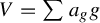 $V = \sum a_g g$
, then
 $$ \begin{align*} V|\textbf{S} = \sum a^{\prime}_g g, \end{align*} $$
where
 $a^{\prime }_g = a_g$
if
 $\eta (g) = 0$
for some
 $\eta $
in the relative interior of
 $\mathbb {R}_+\textbf {S}$
and
 $a^{\prime }_g = 0$
otherwise (cf. Proposition 7.6). We note that this definition does not depend on the choice of
 $\eta $
in the relative interior of
 $\mathbb {R}_+\textbf {S}$
. This follows from the fact that the cone of homology directions
 $\mathrm {cone}_1(\Gamma )$
and
 $\mathrm {cone}_2(\tau )=\mathbb {R}_+\textbf {F}$
are dual (Theorem 2.2(2)). Indeed, the basic theory of convex polyhedral cones in finite-dimensional vector spaces (see e.g. [Reference FultonFul93, §1.2]) gives that if
 $\eta ,\eta '$
are two classes lying in the relative interior of
 $\mathbb {R}_+\textbf {S}$
, then
 $\ker (\eta )\cap \mathrm {cone}_1(\Gamma )=\ker (\eta ')\cap \mathrm {cone}_1(\Gamma )$
.
In this setting, Theorems 7.1 and 7.2 easily imply the following.
Corollary 9.8. (Counting orbits missing transverse surfaces)
Suppose that M has a fully punctured fibered face
 $\textbf {F}$
. Let
 $\tau $
be the associated veering triangulation and
 $\varphi $
the associated suspension flow. Finally, fix a subface
 $\textbf {S}$
of
 $\textbf {F}$
and let
 $\eta \in \operatorname {\mathrm {int}} (\mathbb {R}_+\textbf {S})$
.
For any
 $\xi \in \operatorname {\mathrm {int}}(\mathbb {R}_+\textbf {F})$
, the growth rate
 $$ \begin{align} \mathrm{gr}_{\varphi}(\xi; \textbf{S}) = \lim_{L\to \infty} \# \{ \gamma \in \mathcal O_{\varphi} : \eta(\gamma) =0 \text{ and } \xi(\gamma) \le L \} ^{{1}/{L}} \end{align} $$
exists and equals the reciprocal of the smallest root of the specialization
 $V|\textbf {S}^{\xi }$
.
Moreover, the following hold.
-
(1) The growth rates
$\mathrm {gr}_{\varphi }(\xi; \textbf {S})$
depend only on the face
$\textbf {S}$
and not the chosen
$\eta $
. -
(2) If S is any surface carried by
$\tau $
dual to a class in
$\operatorname {\mathrm {int}} (\mathbb {R}_+\textbf {S})$
, then
$\mathrm {gr}_{\varphi }(\xi; \textbf {S})$
computes the growth rate (with respect to
$\xi $
) of closed orbits that miss the surface S and is equal to
$\mathrm {gr}_{\varphi |S}(\xi )$
from equation (7.1). -
(3) The growth rate
$\mathrm {gr}_{\varphi }(\xi; \textbf {S})$
is strictly larger than
$1$
if and only if there are infinitely many primitive closed orbits that are
$\eta $
-null.


We remark that a straightforward calculation shows that
 $V|S\in \mathbb {Z}[H_1(M)/\text {torsion}]$
is equal to the image of
 $P_{\Phi |S}$
under the map induced by the inclusion
 $\Phi |S\to M|S\to M$
, regardless of whether
 $\textbf {F}$
is fibered. However, for
 $V|S$
to output interesting dynamical information as in the above result, the fibered hypothesis is essential: there exists a class
 $\xi \in H_1(M)$
which pulls back to a positive class on
 $M| S$
if and only if
 $\textbf {F}$
is fibered. For the less trivial direction of this statement, note that if
 $\xi \in H^1(M)$
is a class pairing positively with every closed orbit that has zero pairing with
 $\eta $
, then
 $\xi +k\eta $
pairs positively with every closed orbit of
 $\varphi $
for sufficiently large k. As a consequence,
 $\xi +k\eta $
is dual to a cross section to
 $\varphi $
.
Also, we again emphasize that Corollary 9.8 has a natural generalization to closed manifolds by first puncturing along singular orbits of the suspension flow.
Remark 9.9. Depth one foliations and stretch factors of endperiodic monodromies
The growth rates appearing in Corollary 9.8 when
 $\xi $
is integral can be naturally interpreted as stretch factors of endperiodic homeomorphisms associated to depth one foliations of M (or more precisely, its compact model as in Remark 4.6). Indeed, if S is a surface carried by
 $\tau $
that is not a fiber, then any primitive integral class
 $\xi $
in the interior of the associated fibered cone gives rise to a depth one taut oriented foliation on
 $M|S$
that is positively transverse to flow lines of
 $\varphi $
(see for example [Reference AgolAgo08, Theorem 3.7]). The foliation restricted to the complement of the boundary (depth zero) leaves is a fibration over the circle and the first return map to a fiber (that is, a depth one leaf) is a endperiodic homeomorphism [Reference FenleyFen92, Lemmas 4.1 and 4.2]. The growth rate of periodic points of the first return map is equal to
 $\mathrm {gr}_{\varphi |S}(\xi )$
, giving a direct generalization of the stretch factor of a pseudo-Anosov homeomorphism. These stretch factors will be the subject of future work [Reference Landry, Minsky and TaylorLMT22].
We can use these tools to answer the following question of Chris Leininger.
Question 1. (Leininger)
Given a fibered face
 $\textbf {F}$
of a hyperbolic
 $3$
-manifold M, what is the limit set of stretch factors arising from monodromies whose fibers correspond to integral points in
 $\mathbb {R}_+ \textbf {F}$
?
It is clear that
 $1$
is such an accumulation point, but in unpublished work, Leininger and Shixuan Li have produced examples where there are accumulation points greater than
 $1$
.
To answer Question 1, we introduce the following notation. For each subface
 $\textbf {S}$
of
 $\textbf {F}$
define
 $$ \begin{align*} \Lambda( \textbf{S}) = \{\mathrm{gr}_{\varphi}(\alpha; \textbf{S}) : \alpha \text{ is an integral point of } \mathrm{int}(\mathbb{R}_+ \textbf{F}) \}, \end{align*} $$
where
 $\mathrm {gr}_{\varphi }(\alpha; \textbf {S})$
is as in equation (9.2). Also set
 $\Lambda = \Lambda ( \emptyset )$
, which is exactly the set of stretch factors of the monodromies of fibrations corresponding to integral points in
 $\mathbb {R}_+ \textbf {F}$
. Our goal is to understand its closure
 $\overline \Lambda $
.
Recall that
 $X^{\prime }$
denotes the derived set of X, that is, its set of accumulation points. Also inductively set
 $X^0 = X$
and
 $X^{n+1} = (X^n)^{\prime }$
.
Theorem 9.10. (Structure of stretch factors)
Let
 $\Lambda \subset (1,\infty )$
be the set of stretch factors of the monodromies of fibrations corresponding to integral points in
 $\mathbb {R}_+ \textbf {F}$
. Then its closure
 $\overline \Lambda $
is compact, well ordered under
 $\ge $
, and
 ${\overline \Lambda }^n = \{1\}$
for some
 $1\le n \le \mathrm {dim} (H^1(M; \mathbb {R}))$
.
Moreover:
-
• each number in
$\overline \Lambda ^{\prime } \smallsetminus \{1\}$
is itself a growth rate in the sense of Corollary 9.8 and an infinite type stretch factor in the sense of Remark 9.9; -
• the accumulation set
$\overline \Lambda ^{\prime }$
is infinite if and only if there are infinitely many primitive orbits in
$\mathcal O_{\varphi }$
that are null with respect to some class in
$\partial (\mathbb {R}_+\textbf {F})$
; and -
• the derived length is maximal (that is,
$n = \mathrm {dim} (H^1(M; \mathbb {R}))$
) if and only if there are infinitely many primitive orbits in
$\mathcal O_{\varphi }$
that represent a multiple of a vertex class in the cone of homology directions in
$H_1(M; \mathbb {R})$
.


Proof. In the proof, we assume that the fibered face
 $\textbf {F}$
is fully punctured and associated to the veering triangulation
 $\tau $
of M. The general case then follows from puncturing along singular orbits and considering only cohomology pulled back from the original manifold.
We begin by establishing a more technical claim.
Claim 9.11. (going up)
Let
 $\textbf {S}$
be a face of
 $\textbf {F}$
. Then
 $$ \begin{align*} \overline {\Lambda( \textbf{S})}^{\prime} \smallsetminus \{1\} = \bigcup_{\textbf{T}\supset \textbf{S}} \Lambda( \textbf{T}) \smallsetminus\{1\}, \end{align*} $$
where the union is over proper faces
 $\textbf {T}$
of
 $\textbf {F}$
that properly contain
 $\textbf {S}$
.
Moreover, if
 $(\unicode{x3bb} _k)$
is a sequence in
 $\Lambda ( \textbf {S})$
converging to
 $\unicode{x3bb} \in \overline {\Lambda ( \textbf {S})}^{\prime }$
, then
 $\unicode{x3bb} \le \unicode{x3bb} _k$
for sufficiently large k.
Proof of claim
Any integral
 $\alpha $
in the interior of
 $\mathbb {R}_+ \textbf {F}$
can be realized as a (multiple of a) fiber surface
 $S_{\alpha }$
carried by
 $\tau $
. We note that while the isotopy class of
 $S_{\alpha }$
is unique, its carried position is not, but this will not matter here. Since the image of
 $\Phi $
in M is positively transverse to
 $\tau ^{(2)}$
, the non-negative integral cocycle
 $m_{\alpha }$
on
 $\Phi $
given by mapping each directed edge to its intersection number with
 $S_{\alpha }$
represents the pullback of
 $\alpha $
to
 $\Phi $
. Obviously, the restriction of
 $m_{\alpha }$
to any subgraph of
 $\Phi $
represents the pullback of
 $\alpha $
to that subgraph.
We first prove the containment
 $\Lambda ( \textbf {T}) \smallsetminus \{1\} \subset \overline {\Lambda ( \textbf {S})}^{\prime } \smallsetminus \{1\}$
for each
 $\textbf {T} \supset \textbf {S}$
. Fix an integral class
 $\eta $
in the relative interior of
 $\mathbb {R}_+\textbf {T}$
, and let
 $\Phi |\textbf {T} = \Phi |\eta $
be the subgraph of
 $\Phi $
covered by cycles that are
 $\eta $
-null (as in §7.1). Also fix
 $\alpha \in \mathrm {int}(\mathbb {R}_+\textbf {F})$
so that
 $\mathrm {gr}(\alpha; \Phi |\textbf {T})>1$
. For
 $i>0$
, we note that
 $\alpha + i\eta $
and
 $\alpha $
agree on cycles of
 $\Phi |\textbf {T}$
, while the value of
 $\alpha + i\eta $
on any cycle of
 $\Phi |\textbf {S}$
not contained in
 $\Phi |\textbf {T}$
goes to
 $\infty $
with i. At this point, we use the following lemma about growth rates in graphs. It is probably well known, but for completeness, we will include a proof at the end.
For a directed graph D and positive class
 $\alpha \in H^1(D)$
(that is, class that is positive on directed cycles), let
 $\mathrm {gr}(\alpha ;D)$
denote the growth rate of directed cycles in D with respect to
 $\alpha $
(as in equation (7.2)).
Lemma 9.12. Let D be a directed graph with subgraph
 $D'$
. Let
 $\alpha _i$
be a sequence of positive classes in
 $H^1(D)$
that pull back to the same positive class
 $\alpha \in H^1(D')$
. Then,
 $$ \begin{align*} \mathrm{gr}(\alpha_i; D) \ge \mathrm{gr}(\alpha; D'). \end{align*} $$
Suppose further that:
-
(1) the
$\alpha _i$
blow up on the complement of
$D'$
(that is,
$\alpha _i(\gamma ) \to \infty $
for each directed cycle
$\gamma $
of D that is not contained in
$D'$
); and -
(2)
$\liminf _{i \to \infty } \mathrm {gr}(\alpha _i; D )> 1$
.



Then,
 $$ \begin{align*} \mathrm{gr}(\alpha_i; D) \to \mathrm{gr}(\alpha; D') \end{align*} $$
as
 $i \to \infty $
.
We apply Lemma 9.12 to conclude that
 $\mathrm {gr}(\alpha + i \cdot \eta; \Phi |\textbf {S}) \ge \mathrm {gr}(\alpha; \Phi |\textbf {T})> 1$
and that
 $$ \begin{align*} \mathrm{gr}(\alpha + i \cdot \eta; \Phi|\textbf{S}) \to \mathrm{gr}(\alpha; \Phi|\textbf{T}) \end{align*} $$
as
 $i\to \infty $
, and note that this sequence is non-constant exactly when the containment
 $\textbf {T} \supset \textbf {S}$
is proper. By Theorem 7.1 (and Corollary 9.8(2)), this gives us
 $$ \begin{align*} \mathrm{gr}_{\varphi}(\alpha + i \cdot \eta; \textbf{S}) \to \mathrm{gr}_{\varphi}(\alpha; \textbf{T}). \end{align*} $$
Thus, any point of
 $\Lambda (\textbf {T})$
is a limit point of
 $\Lambda (\textbf {S})$
.
Conversely, let
 $\alpha _i \in \mathrm {int}(\mathbb {R}_+\textbf {F})$
be a sequence of integral classes so that the sequence of growth rates
 $\unicode{x3bb} _i = \mathrm {gr}_{\varphi }(\alpha _i; \textbf {S})$
is pairwise distinct and converges to
 $\unicode{x3bb}>1$
, and let us show that
 $\unicode{x3bb} \in \Lambda (\textbf {T})$
for some face
 $\textbf {T} \supsetneq \textbf {S}$
.
Now let
 $\eta $
denote an integral class in the relative interior of
 $\mathbb {R}_+\textbf {S}$
(if
 $\textbf {S} = \emptyset $
, then by convention,
 $\eta = 0$
and
 $\Phi |\eta =\Phi |\textbf {S} = \Phi $
). Replace each
 $\alpha _i$
in this sequence with
 $\alpha _i + i \cdot \eta $
. This does not change
 $\unicode{x3bb} _i = \mathrm {gr}(\alpha _i; \textbf {S})$
, but it ensures that
 $\alpha _i (\gamma ) \to \infty $
for any directed cycle of
 $\Phi $
that is not in
 $\Phi |\textbf {S}$
.
After passing to a subsequence, we may assume that for each edge e of
 $\Phi |\textbf {S}$
, either
 $m_{\alpha _i}(e)$
stays bounded for all i or
 $m_{\alpha _i}(e) \to \infty $
. Let E be the set of edges whose lengths stay bounded. Because each
 $m_{\alpha _i}$
is integral, we may pass to a further subsequence and assume that
 $m_{\alpha _i}(e) =: m(e)$
is constant for each edge e of E.
We can again apply Lemma 9.12 to the pullback of
 $\alpha _i$
on the graphs E and
 $\Phi |\textbf {S}$
, concluding
 $$ \begin{align*}\mathrm{gr}(\alpha_i; \Phi|\textbf{S}) \to \mathrm{gr}(\alpha;E). \end{align*} $$
This limit is then
 $\unicode{x3bb} $
since
 $\mathrm {gr}(\alpha _i; \Phi |\textbf {S}) = \mathrm {gr}_{\varphi }(\alpha _i;\textbf {S})$
by Theorem 7.1 and Corollary 9.8. Since
 $\unicode{x3bb}>1$
, E has a non-trivial recurrent subgraph. It remains to find a face
 $\textbf {T}$
strictly containing
 $\textbf {S}$
such that
 $\mathrm {gr}(\alpha ;E) = \mathrm {gr}(\alpha ;\Phi |\textbf {T})$
.
Set
 $\eta _i = \alpha _i - \alpha _1$
. We claim that for i sufficiently large,
 $\eta _i$
is contained in the relative interior of
 $\mathbb {R}_+\textbf {T}$
for some face
 $\textbf {T}$
that properly contains
 $\textbf {S}$
. Let
 $\gamma $
be a directed cycle in
 $\Phi $
. If
 $\gamma $
is not contained in
 $\Phi |\textbf {S}$
, then
 $\eta (\gamma )>0$
and so
 $\alpha _i(\gamma ) \to \infty $
by definition of
 $\eta $
. Hence,
 $\eta _i(\gamma )>0$
for large i. If
 $\gamma $
is contained in
 $\Phi | \textbf {S}$
but not in E, then again
 $\alpha _i(\gamma )\to \infty $
by definition of E so
 $\eta _i(\gamma )> 0$
for large i. If
 $\gamma $
is contained in E, then
 $\alpha _i(\gamma ) = \alpha _1(\gamma )$
so
 $\eta _i(\gamma )=0$
. At any rate,
 $\eta _i(\gamma ) \ge 0$
and since the cone of homology directions is spanned by finitely many cycles in
 $\Phi $
(Theorem 2.2), we may fix i so that
 $\eta _i \in \mathbb {R}_+ \textbf {F}$
.
Let
 $\textbf {T}$
be the face of
 $\textbf F$
such that
 $\eta _i$
is in the relative interior of
 $\mathbb {R}_+{\textbf T}$
. Then from the previous paragraph, we see that E and
 $\Phi |{\textbf T}$
have the same directed cycles, namely those where
 $\eta _i$
vanishes. Thus,
 $\mathrm {gr}(\alpha ;E) = \mathrm {gr}(\alpha ;\Phi |\textbf {T})$
, and the latter equals
 $\mathrm {gr}_{\varphi }(\alpha ;\textbf T)$
by Theorem 7.1. Note that
 $\textbf S$
is a proper subface of
 $\textbf T$
because we have assumed the
 $\unicode{x3bb} _i$
are not eventually constant.
Applying this to all limit points
 $\unicode{x3bb} $
, we obtain the containment
 $$ \begin{align*} \overline {\Lambda( \textbf{S})}^{\prime} \smallsetminus \{1\} \subset \bigcup_{\textbf{T}\supsetneq \textbf{S}} \Lambda( \textbf{T}) \smallsetminus\{1\}. \end{align*} $$
The final statement, that eventually
 $\unicode{x3bb} _i \ge \unicode{x3bb} $
, follows from the first conclusion of Lemma 9.12, and the fact that
 $\unicode{x3bb} _i = \mathrm {gr}(\alpha _i;\Phi |\textbf S)$
again by Theorem 7.1. This concludes the proof of Claim 9.11.
The claim now immediately implies that
 $\overline \Lambda $
is well ordered by
 $\geq $
and that the length of the derived sequence is bounded above by
 $\mathrm {dim} (H^1(M; \mathbb {R}))$
. Compactness of
 $\overline \Lambda $
was previously observed by Leininger (see also [Reference FriedFri82a, Theorem A]), but it also follows from our setup. First recall that as in the proof of Claim 9.11, the pullback to
 $\Phi $
of each integral class
 $\alpha $
in
 $\mathbb {R}_+\textbf {F}$
can be represented by a non-negative, integral cocycle
 $m_{\alpha }$
that is positive on directed cycles of
 $\Phi $
. By Theorem 7.1, to show that
 $\Lambda $
is bounded above, it suffices to show that
 $\mathrm {gr}_{\Phi }([m])$
is uniformly bounded over all non-negative, integral cocycles m representing a positive class
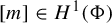 $[m]\in H^1(\Phi )$
. This is straightforward: if m is such a cocycle, then we obtain another such cocycle
 $m'$
by declaring that
 $m'(e) =0$
if
 $m(e)=0$
and
 $m'(e)=1$
otherwise, for each directed edge e of
 $\Phi $
. Since m is integral and non-negative,
 $m'(e) \le m(e)$
for all directed edges e of
 $\Phi $
. This implies that
 $\mathrm {gr}_{\Phi }([m]) \le \mathrm {gr}_{\Phi }([m'])$
. However, since there are only finitely many cocycles taking values in
 $\{0,1\}$
, there is a maximum to their growth rates (after restricting to those that are positive on directed cycles). Hence,
 $\Lambda $
is bounded and so
 $\overline \Lambda $
is compact.
It only remains to prove the additional items. The first item follows from the proof of Claim 9.11. The second item follows from Corollary 9.8(3), since if
 $(\alpha _i)$
is a sequence of classes with
 $\mathrm {gr}(\alpha _i)\to x>1$
, then for all
 $n\in \mathbb {N}$
, we have
 $\mathrm {gr}(n\alpha _i)=\mathrm {gr}(\alpha _i)^{{1}/{n}}\to x^{{1}/{n}}$
. Finally, for the third item, it is easy to see (again by Corollary 9.8(3)) that the derived length is maximal if and only if for some
 $\eta $
in the relative interior of a top dimensional face
 $\textbf {S}$
of
 $\textbf {F}$
, there are infinitely many closed primitive orbits that are
 $\eta $
-null. All such orbits must represent a multiple of the vertex of the cone of homology directions that is dual to
 $\mathbb {R}_+\textbf {S}$
. This completes the proof of Theorem 9.10.
We conclude with a proof of Lemma 9.12. Instead of assuming that the
 $\alpha _i$
pull back to the same class on
 $D'$
, it in fact suffices to assume that the pullbacks to
 $H^1(D')$
converge, but we will only need the weaker statement. Also, condition
 $(2)$
could be replaced by the condition that
 $\mathrm {gr}(\alpha; D') \ge 1$
, that is, that
 $D'$
contains a directed cycle, but we have chosen to state Lemma 9.12 so that it can be directly applied in the proof of Theorem 9.10.
Proof of Lemma 9.12
Set
 $\unicode{x3bb} _i = \mathrm {gr}(\alpha _i; D)$
and
 $\unicode{x3bb} = \mathrm {gr}(\alpha; D')$
. Clearly,
 $\unicode{x3bb} \le \unicode{x3bb} _i$
since
 $D' \subset ~D$
.
Now assume items
 $(1)$
and
 $(2)$
from the lemma statement. We claim that
 $\unicode{x3bb} _i$
are bounded above: for i sufficiently large,
 $\alpha _i(\gamma ) \ge \alpha _1(\gamma )$
for all directed cycles
 $\gamma $
of D and this implies that
 $\mathrm {gr}(\alpha _i; D) \le \mathrm {gr}(\alpha _1; D)$
. Thus, it suffices to show that any accumulation point
 $\mu \ge \unicode{x3bb} $
of
 $(\unicode{x3bb} _i)$
is equal to
 $\unicode{x3bb} $
.
Let
 $P_D$
be the Perron polynomial of D. From equation (2.2), we see that this is a sum
 $$ \begin{align*} P_D = P_{D'} + N, \end{align*} $$
where
 $P_{D'}$
is the Perron polynomial of
 $D'$
consisting of the terms of
 $P_D$
that correspond to cycles contained in
 $D'$
and where N has terms corresponding to cycles that are not contained in
 $D'$
. Specializing (as in §2.3), we get
 $$ \begin{align*} P_D^{\alpha_i}(t^{-1}) = P_{D'}^{\alpha}(t^{-1}) + N^{\alpha_i}(t^{-1}), \end{align*} $$
where the largest real root of
 $P_D^{\alpha _i}(t^{-1})$
is
 $\unicode{x3bb} _i$
and the largest real root of
 $P_{D'}^{\alpha }(t^{-1})$
is
 $\unicode{x3bb} $
(see [Reference McMullenMcM15, Theorem 1.2]), unless
 $D'$
contains no directed cycles. In this last case, we would have that
 $P_{D'} = 1$
and
 $\unicode{x3bb} = 0$
.
Since the
 $\alpha _i$
blow up on loops not in
 $D'$
,
 $N^{\alpha _i}(t^{-1})$
is a finite sum of terms of the form
 $a t^{-x_i}$
, where
 $x_i \to \infty $
as
 $i \to \infty $
.
Let
 $\mu $
be an accumulation point of
 $(\unicode{x3bb} _i)$
. Then
 $\mu \ge \unicode{x3bb}> 1$
. Passing to a subsequence, we may assume
 $\unicode{x3bb} _i \to \mu $
, and plugging into the specializations, we obtain
 $$ \begin{align*} 0 = P_{D'}^{\alpha}(\unicode{x3bb}_i^{-1}) + N^{\alpha_i}(\unicode{x3bb}_i^{-1}). \end{align*} $$
Then using the above description of
 $N^{\alpha _i}$
and that fact that
 $\unicode{x3bb} _i \to \mu>1$
, we see that
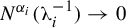 $N^{\alpha _i}(\unicode{x3bb} _i^{-1}) \to 0$
as
 $i \to \infty $
. So by continuity of
 $P_{D'}^{\alpha }(t^{-1})$
, we get that
 $\mu $
is a root of
 $P_{D'}^{\alpha }(t^{-1})$
. Since
 $\unicode{x3bb} $
is the largest root, we conclude
 $\mu = \unicode{x3bb} $
. This completes the proof of Lemma 9.12.
Acknowledgements
We thank Chris Leininger for illuminating discussions on the topic and for asking Question 1, Amie Wilkinson for helpful remarks related to §5.9, and Chi Cheuk Tsang for comments on an earlier draft. This work was partially supported by the NSF postdoctoral fellowship DMS-2013073, NSF grants DMS-1744551, DMS-2005328, DMS-2102018, and the Sloan Foundation.