Nomenclature
altitude cost
- UAV
-
unmanned aerial vehicle
- GWO
-
grey wolf optimiser
- CGWO
-
chaotic grey wolf optimiser
- S
-
origin
- E
-
destination
-
 ${d_T}$
-
horizontal distance from the UAV to the obstacle’s centre
-
${d_{Tmin}}$
-
minimum distance limit between the UAV and the obstacle
-
${h_i}$
-
height of UAVs
-
${h_{saf{e_i}}}$
-
safety height
-
${L_i}$
-
trajectory distance of the
$i$
th drone -
${v_{max}},{v_{min}}$
-
maximum and minimum speed
- K
-
number of peaks
- m
-
number of sampling points
- M
-
number of UAVs
- n
-
number of waypoints
- t
-
number of iterations
- T
-
Maximum iterations
-
${O_{fuel}}$
-
fuel cost
-
${O_{threat}}$
-
threat cost
-
${O_{angle}}$
-
angle cost
-
${O_{height}}$
-
redaltitude cost
-
${O_{time}}$
-
time cost
-
${O_{dis}}$
-
distance cost


Greek symbol
-
$\alpha $
-
the ratio of the overlapping time interval of the two UAVs
-
$\omega $
-
weighting factor
-
$\theta $
-
slope of the peak
-
${\beta _i},{\varphi _{}}$
-
climbing angle and steering angle
-
$\mu $
-
control parameter


1.0 Introduction
In the past few years, the swift advancements in UAV technology have revolutionised multiple sectors [Reference Arik, Turkmen and Oktay1, Reference Oktay and Coban2]. From military surveillance and environmental assessments to traffic oversight and disaster relief efforts, UAVs have become indispensable tools across diverse industries [Reference Yesilbas, Özgür, Ozen and Oktay3, Reference Oktay, Arik, Turkmen, Uzun and Celik4]. However, the efficient planning of UAV flight paths, especially in multi-UAV cooperative operations, remains a challenging research problem. Multi-UAV path planning not only requires individual UAVs to be able to accomplish their respective tasks, but must also consider variables like UAV teamwork, collision prevention and power usage. Therefore, how to realise efficient collaboration and trajectory optimisation for multiple UAVs in intricate settings has emerged as a key focus in contemporary UAV studies [Reference Xu, Cao, Du and Li5–Reference Uzun and Oktay8].
Nowadays commonly used multi-UAV path planning algorithms include traditional path planning algorithms based on graph search, intelligent optimisation algorithms and fusion algorithms based on reinforcement learning. Traditional path planning algorithms are mainly based on graph search, which mainly include Dijkstra algorithm, A-star algorithm [Reference Hart, Nilsson and Raphael9], breadth-first search (BFS) algorithm [Reference Beamer, Asanović and Patterson10] and rapidly exploring random trees (RRT) algorithm [Reference LaValle11]. However, traditional road path planning algorithms are usually only applicable to simple scenarios and have poor computational efficiency and flexibility when facing dynamic obstacles and complex environments. Intelligent optimisation algorithms are modeled after natural or social phenomena that simulate their behaviour or mechanisms to solve optimisation problems. Compared with traditional algorithms, intelligent optimisation algorithms possess robust global search abilities, making them appropriate for intricate, nonlinear and large-scale optimisation challenges. Common intelligent optimisation algorithms include particle swarm optimisation algorithm (PSO) [Reference Kennedy and Eberhart12], genetic algorithm (GA) [Reference Lambora, Gupta and Chopra13], differential evolutionary (DE) algorithm [Reference Storn and Price14], immune plasma algorithm (IPA) [Reference Aslan, Demirci, Oktay and Yesilbas15], grey wolf optimisation (GWO) [Reference Mirjalili, Mirjalili and Lewis16], and others. Currently, various meta-heuristic algorithms have been applied to solve drones’ path planning problems. Reference [Reference Dasdemir, Köksalan and Öztürk17] proposes a preference-based evolutionary algorithm for constrained multi-UAV path planning. Reference [Reference He, Qi and Liu18] combines PSO with an improved symbiotic method, thereby solving the problem of cooperative paths for multi-UAV. Reference [Reference Aslan and Oktay19] uses a newly proposed method called extended treatment approach to improve the IPA and applies it to aircraft path planning, resulting in a significant improvement in path quality.
The GWO is suitable for complex, nonlinear and unstructured optimisation problems, which not only possesses strong global search capability, but also low parameter adjustment demand, simple implementation and strong adaptability, which makes it has great flexibility in practical application. However, the GWO suffers from a problem that increases the probability of being confined to local optima and results in slower convergence. Reference [Reference Shi, Tan, Zhang, Lian and Xu20] proposes a spiral position update technique using GWO, assigning the golden ratio as its probability parameter. Reference [Reference Huang, Jiang, Wu, Liu, Dong and Ping21] introduces a nonlinear convergence factor and a levy on-the-fly update strategy to enhance the optimisation of the algorithm. Reference [Reference Lv and Wang22] combines GWO with DE, optimising the equilibrium of algorithmic evolution and search. Nonlinear transformations of parameters enhance algorithmic performance.
In this paper, CGWO is introduced to address multi-UAV path planning in intricate environments. In the initialisation phase, chaotic initialisation is used instead of random initialisation to enhance population diversity and stop the algorithm from converging to local optima. During the iteration of the algorithm, chaotic local search is introduced to improve local search diversity and exploration, preventing premature convergence to the local optimal solution. In addition, the leader dynamic reduction mechanism is used in the following phase to provide a balanced adaptive search for both global and local optimisation, enhancing the algorithm’s convergence rate and precision.
2.0 Modeling cooperative path planning for multi-uav
During UAV route optimisation, we need to consider a variety of constraints. In multi-UAV path planning, the first step is to model the flight environment and establish an environment model based on it. Then, define
 $S$
as the origin,
 $E$
as the destination, with
 $N$
intermediate points composing the UAV’s trajectory
 $\left\{ {S,{P_1},{P_2}, \ldots ,{P_n},E} \right\}$
. In this study, the multi-UAV path planning problem is modeled as a labeled path generation problem, where each UAV is assigned a specific origin and destination. A feasible path from the origin to the destination must be generated for each UAV while satisfying flight safety and path feasibility constraints. Considering various constraints, the multi-UAV path cost function is established as a measure for assessing path quality. The path cost function mainly encompasses fuel cost, threat cost, altitude cost, angle cos, and cooperation cost [Reference Xu, Cao, Du and Li5]. The cooperation cost includes time cost and distance cost. The objective function for collaborative multi-UAV routing is:
 \begin{align}O = {\omega _1} \cdot {O_{fuel}} + {\omega _2} \cdot {O_{threat}} + {\omega _3} \cdot {O_{angle}} + {\omega _4} \cdot {O_{height}} + {\omega _5} \cdot {O_{time}} + {\omega _6} \cdot {O_{dis}}\end{align}
where
 ${\omega _1}$
,
 ${\omega _2}$
,
 ${\omega _3}$
,
 ${\omega _4}$
,
 ${\omega _5}$
and
 ${\omega _6}$
represent weighting coefficients for differernt cost functions and sum to one. By adjusting the value of the weighting coefficient, the UAV flight path satisfying different requirements can be obtained [Reference Thoma, Thomessen, Gardi, Fisher and Braun23].
2.1 Flight environment
In multi-UAV route planning, it is necessary to establish a suitable planning space according to the flight environment. In the current work, the task working environment is set to mountain, and elevation data, simulating mountain hazards, comes from a stochastically generated digital terrain model [Reference Cheng, Tang and Liu24]. This model includes the raw digital model and the threat equivalent terrain model, where the raw data model is represented as
 \begin{align} {z_1}\!\left( {x,y} \right) = {\rm{sin}}\!\left({y + a} \right) + b \cdot {\rm{sin}}\!\left(x \right) + c \cdot {\rm{cos}}\!\left({d \cdot \sqrt {{x^2} + {y^2}} } \right)\nonumber\\+ e \cdot {\rm{cos}}\!\left(y \right) + f \cdot {\rm{sin}}\!\left({f \cdot \sqrt {{x^2} + {y^2}} } \right) + g \cdot {\rm{cos}}\!\left(y \right)\end{align}
where
 $x$
and
 $y$
represent the coordinates of the horizontal projection of the original digital model;
 ${z_1}$
denotes elevation within the X-Y plane;
 $a,b,c,d,e,f$
and
 $g$
represent constants, and diverse landscapes can be achieved by adjusting these coefficient values.
The terrain model of threat equivalence is
 \begin{align}{z_2}\!\left({x,y} \right) = \mathop \sum \limits_{i = 1}^K h\!\left( i \right) \cdot exp\!\left( { - {{\left( {{{x - {x_{0i}}} \over {{x_{si}}}}} \right)}^2} - {{\left( {{{y - {y_{0i}}} \over {{y_{si}}}}} \right)}^2}} \right)\end{align}
where
 $x$
and
 $y$
represent the horizontal coordinates of the threat equivalent terrain projection;
 ${z_2}$
denotes the elevation linked to the horizontal axis in the threat equivalence framework. The height of peak
 $i$
is denoted by
 $h\!\left( i \right)$
, while its apex is located at the coordinates (
 ${x_{0i}},{y_{0i}}$
). The variables
 ${x_{si}}$
and
 ${y_{si}}$
represent parameters that influence the gradient of peak
 $i$
on the X and Y axes, respectively. When
 ${x_{si}}$
and
 ${y_{si}}$
take on larger values, the slope of the peak becomes more gradual.
The ultimate obstacle model merges the initial digital model with the threat-equivalent terrain model, selecting the higher value between the two.
 \begin{align}z\!\left({x,y}\right) = {\rm{max}}\!\left[{{z_1}\!\left({x,y}\right),{z_2}\!\left({x,y}\right)} \right]\end{align}
Various landscapes can be generated by adjusting the function’s parameters. The 3D terrain planning environment is shown in Fig. 1.
The 3D terrain planning environment.

2.2 Threat cost
During UAV path planning, the UAV must steer clear of obstacles. In this paper, the obstacles are the peaks, modeled as cones, and the paths formed between two adjacent waypoints of the UAV should avoid the peaks. Between every two waypoints, it is split into
 $m + 1$
segments to obtain
 $m$
sampling points, and the threat cost between two adjacent waypoints is calculated according to
 $m$
sampling points. At the same time, the height condition is set, when the UAV’s altitude exceeds the mountain’s peak height, the threat cost of the UAV is 0, and the UAV flight safety is guaranteed by its altitude.
The threat cost function of UAV is calculated as follows:
 \begin{align}{O_{threat}} &= \mathop \sum \limits_{i = 0}^n \mathop \sum \limits_{j = 0}^m \mathop \sum \limits_{k = 1}^K threa{t_{ij}}\left( k \right) \end{align}
 \begin{align} threa{t_{ij}}\!\left(k \right) &= \left\{ {\begin{array}{l@{\quad}l}0 & {{{\rm{h}}_{\rm{j}}} \gt H\!\left(k\right)\ \textrm{or}\ {\rm{\Delta d}} \gt {{\rm{R}}_{\rm{T}}}} \\[3pt] \nonumber {{R_T} - {\rm{\Delta }}d} & {{{\rm{h}}_{\rm{j}}} \lt H\!\left(k \right)\ \textrm{and}\ {\rm{\Delta d}} \lt {{\rm{R}}_{\rm{T}}}}\end{array}} \right. \end{align}
 \begin{align}{\rm{\Delta }}d &= {d_T} - {d_{Tmin}} \end{align}
 \begin{align}{R_T} &= \left( {H\!\left(k \right) - {h_j}} \right)/tan\theta \\[8pt] \nonumber \end{align}
where
 $H\!\left(k \right)$
denotes peak
 $k$
’s height and
 ${h_j}$
represents the UAV’s flight altitude;
 ${R_T}$
refers to the obstacle radius corresponding to the current UAV’s altitude, and
 $\theta $
represents the incline of the current mountain obstacle;
 ${d_T}$
denotes the horizontal distance from the UAV to the obstacle’s centre;
 ${d_{Tmin}}$
is the minimum distance limit between the UAV and the obstacle that is feasible for obstacle avoidance. The diagram of obstacle avoidance is shown in Fig. 2.
Diagram of obstacle avoidance.

2.3 Fuel cost
In the UAV route optimisation challenge, fuel consumption is the primary concern. UAV flight path distance directly impacts fuel consumption. The fuel cost function is proportional to the path length. Therefore, minimising fuel consumption means minimising the path length of the UAV. As can be seen from the above, a series of N waypoints has been established between the UAV’s launch and landing sites. By determining the Euclidean distance between each pair of neighbouring waypoints, we can accurately approximate the drones’ overall trajectory distances. The UAV’s fuel cost is determined by the formula:
 \begin{align}{O_{fuel}} = \mathop \sum \limits_{i = 0}^n \sqrt {{{\left( {{x_{i + 1}} - {x_i}} \right)}^2} + {{\left( {{y_{i + 1}} - {y_i}} \right)}^2} + {{\left( {{z_{i + 1}} - {z_i}} \right)}^2}} \end{align}
where (
 ${x_i}$
,
 ${y_i}$
,
 ${z_i}$
) and (
 ${x_{i + 1}}$
,
 ${y_{i + 1}}$
,
 ${z_{i + 1}}$
) represent the 3D positions of the current and next waypoints, respectively. (
 ${x_0}$
,
 ${y_0}$
,
 ${z_0}$
) denotes the initial position, (
 ${x_{n + 1}}$
,
 ${y_{n + 1}}$
,
 ${z_{n + 1}}$
) denotes the final position.
2.4 Angle cost
Angle cost is an important metric used to evaluate and optimise the smoothness of the route in UAV path planning. By calculating the angle of steering and climbing between two adjacent waypoints in the UAV path, the path can be ensured to be as smooth as possible in the path optimisation process, thus improving flight efficiency and safety. Where the steering angle is
 $\varphi $
, the climbing angle is
 $\beta $
.
The angle cost is calculated as follows:
 \begin{align} {O_{angle}} &= \mathop \sum \limits_{i = 0}^n \left( {{\beta _i} + {\varphi _i}} \right) \end{align}
 \begin{align} {\beta _{}} &= \left| {{\rm{arctan}}\!\left( {\frac{{\left| {{z_{i + 1}} - {z_i}} \right|}}{{\sqrt {{{\left( {{x_{i + 1}} - {x_i}} \right)}^2} + {{\left( {{y_{i + 1}} - {y_i}} \right)}^2}} }}} \right)} \right| \\[-10pt] \nonumber \end{align}
 \begin{align} {\varphi _i} &= \left| {{\rm{arctan}}\!\left( {\frac{{{y_{i + 1}} - {y_i}}}{{{x_{i + 1}} - {x_i}}}} \right)} \right| \\[8pt] \nonumber \end{align}
where (
 ${x_i}$
,
 ${y_i}$
,
 ${z_i}$
) and (
 ${x_{i + 1}}$
,
 ${y_{i + 1}}$
,
 ${z_{i + 1}}$
) correspond to the 3D coordinates of the current waypoint and the next waypoint.
2.5 Altitude cost
During the flight of the UAV, it must always maintain the altitude within a certain range to ensure the safety of the UAV. The altitude cost is calculated as follows:
 \begin{align} {O_{height}} &= \mathop \sum \limits_{i = 1}^n {\rm{\Delta }}h\!\left( i \right) \end{align}
 \begin{align} {\rm{\Delta }}h\!\left(i \right) &= \left \{ {\begin{array}{l@{\quad}l}{{h_i} - {h_{saf{e_i}}}} & {}{{\rm{if}}\ {{\rm{h}}_{\rm{i}}} \gt {{\rm{h}}_{{\rm{saf}}{{\rm{e}}_{\rm{i}}}}}} \\[3pt] {200 \cdot \left( {{h_{saf{e_i}}} - {h_i}} \right)} {}& {{\rm{otherwise}}}\end{array}} \right. \\[9pt] \nonumber \end{align}
where
 ${h_{saf{e_i}}}$
represents the safety height of the
 $i$
th waypoint. It can be calculated from Equations (2–4),
 ${h_{saf{e_i}}}$
can be expressed by the following equation:
 \begin{align}{h_{saf{e_i}}} = z\!\left({{x_i},{y_i}} \right) = {\rm{max}}\!\left[{{z_1}\!\left({{x_i},{y_i}} \right),{z_2}\!\left({{x_i},{y_i}} \right)} \right]\end{align}
where
 $z\!\left({{x_i},{y_i}} \right)$
represents the terrain height in the flight environment corresponding to the horizontal coordinates of the waypoint
 $\left( {{x_i},{y_i}} \right)$
.
2.6 Cooperation cost
In this paper, the cooperation cost mainly includes the time cost as well as the multi-UAV distance cost. Temporal cooperation requires that all UAVs arrive at the destination at the same time as possible, and if a certain route does not satisfy the temporal cooperation constraint, the path should be modified. The multi-UAV distance cost requires that the distance between two UAVs must be greater than the minimum distance limit, so as to avoid the collision of multiple UAVs.
The speed of the UAVs is assumed to be within [
 ${v_{min}}$
,
 ${v_{max}}$
] and the
 $i$
th UAV’s time interval is
 ${T_i}$
 $ \in $
[
 ${T_{imin}}$
,
 ${T_{imax}}$
]. Meanwhile, the flight time interval of the
 $j$
th UAV is
 ${T_j}$
 $ \in $
[
 ${T_{jmin}}$
,
 ${T_{jmax}}$
]. If the flight times of two UAVs intersect, then two UAVs satisfy the temporal cooperation condition, that is,
 \begin{align} {T_{inter}} &= {T_i} \cap {T_j} \ne \emptyset \end{align}
 \begin{align} {T_{imin}} &= \frac{{{L_i}}}{{{v_{max}}}} \end{align}
 \begin{align} {T_{imax}} &= \frac{{{L_i}}}{{{v_{min}}}} \\[8pt] \nonumber \end{align}
where
 ${L_i}$
refers to the trajectory distance of the
 $i$
th drone, here replaced by the fuel cost. We define
 ${T_{min}}$
as the minimum time interval for the overall intersection of multiple UAVs. It is set that the ratio of the overlapping time interval of the two UAVs to the shortest interval duration is at least
 $\alpha $
, that is
 ${T_{inter}} \gt \alpha \cdot {T_{min}}$
, we define
 $0 \lt \alpha \le 1$
. The time cost function is as follows:
 \begin{align}{O_{time}} = \left \{ {\begin{array}{l@{\quad}l}{300} & {{{\rm{T}}_{{\rm{inter}}}} = \emptyset }\\[3pt]{300 \cdot \alpha } {}& {0 \lt {{\rm{T}}_{{\rm{inter}}}} \le \alpha \cdot {{\rm{T}}_{{\rm{min}}}}}\\[3pt]0 & {{{\rm{T}}_{{\rm{inter}}}} \gt \alpha \cdot {{\rm{T}}_{{\rm{min}}}}}\end{array}} \right.\end{align}
Multi-UAVs should always pay attention to obstacle avoidance during flight; that is, the distance between any point on the path of two UAVs should be greater than the minimum distance limit. Then the multi-UAV distance cost function is shown as follows:
 \begin{align} {O_{dis}} &= \mathop \sum \limits_{i = 1}^M \mathop \sum \limits_{k = 1}^n {p_{i,k}} \end{align}
 \begin{align} {p_{i,k}} &= \left \{ {\begin{array}{l@{\quad}l}{10} & {{\rm{if}}\ {{\rm{d}}_{{\rm{i}} - {\rm{j}},{\rm{k}}}} \lt {{\rm{d}}_{{\rm{min}}}}} \\[3pt] 0 & {{\rm{otherwise}}}\end{array}} \right. \\[8pt] \nonumber \end{align}
where
 ${p_{i,k}}$
is the penalisation function of the spatial distance of multiple UAVs.
 $m$
denotes the drone count and
 $n$
indicates the path point quantity.
 ${d_{i - j,k}}$
represents distance of the
 $k$
th path point on the
 $i$
th and
 $j$
th UAV trajectories.
 ${d_{min}}$
represents the minimum spatial distance limit between two UAVs.
3.0 The proposed chaotic grey wolf optimiser
To address constrained optimisation during collaborative multi-UAV pathfinding, this study introduces a trajectory planning method utilising CGWO. The algorithm combines the advantages of chaotic mapping and classical GWO, and improves the algorithm’s global and local optimisation performance by improving the population initialisation strategy, local chaotic search and leader optimisation.
3.1 The GWO algorithm
Mirjalili et al. introduced GWO, a swarm-based algorithm mimicking wolf predation [Reference Mirjalili, Mirjalili and Lewis16]. The algorithm mimics the social ranking and predatory tactics observed in wild grey wolves and achieves the solution of complex optimisation problems through simple and efficient rules.
In the GWO, the grey wolf population is categorised into four levels: individual at the highest level is referred to as
 $\alpha $
wolf, the
 $\alpha $
wolf represents the group’s best outcome and is the leader of the entire population, with the main responsibility of being in charge of assisting subjects within a cohort to forage; the suboptimal solution in the population is known as the
 $\beta $
wolf,
 $\beta $
wolf act as assistants to
 $\alpha $
wolf, supplementing
 $\alpha $
wolf to help manage and coordinate pack behaviour; the sub-suboptimal individual in the group is the
 $\delta $
wolf, whose role is to provide advice and offer decision support; individuals in the remaining populations are defined as
 $\omega $
wolves, following the other tier individuals as they move around, regulating internal relationships and ensuring balance within the population.
The hunting formula for wolves is:
 \begin{align} D &= \left| {C \cdot {X_p}\!\left( t \right) - X\!\left( t \right)} \right| \end{align}
 \begin{align} X\!\left({t + 1} \right) &= {X_p}\!\left(t \right) - A \cdot D \end{align}
 \begin{align} A &=\ 2 \cdot a \cdot {r_1} - a \end{align}
 \begin{align} C &=\ 2 \cdot {r_2} \end{align}
 \begin{align} a &=\ 2 - \frac{{2 \cdot t}}{T} \\[8pt] \nonumber \end{align}
where t represents the iteration count;
 $X\!\left(t \right)$
denotes a wolf’s present location;
 ${X_p}\!\left(t \right)$
denotes the prey’s location vector;
 $A$
and
 $C$
are factors;
 ${r_1}$
and
 ${r_2}$
are arbitrary numbers in the interval [0,1];
 $a$
decreases linearly from
 $2$
to
 $0$
.
The remaining grey wolf individuals in the population follow the three wolves with higher priority for position location updates. The positional update formula is:
 \begin{align} {D_\alpha } &= \left| {{C_1} \cdot {X_\alpha }\!\left( t \right) - X\!\left( t \right)} \right| \end{align}
 \begin{align} {D_\beta } &= \left| {{C_2} \cdot {X_\beta }\!\left( t \right) - X\!\left( t \right)} \right| \end{align}
 \begin{align} {D_\delta } &= \left| {{C_3} \cdot {X_\delta }\!\left( t \right) - X\!\left( t \right)} \right| \end{align}
 \begin{align} {X_1} &= {X_\alpha } - {A_1} \cdot {D_\alpha } \end{align}
 \begin{align} {X_2} &= {X_\beta } - {A_2} \cdot {D_\beta } \end{align}
 \begin{align} {X_3} &= {X_\delta } - {A_3} \cdot {D_\delta } \end{align}
 \begin{align} X\!\left( {t + 1} \right) &= \frac{{{X_1} + {X_2} + {X_3}}}{3} \\[8pt] \nonumber \end{align}
where
 ${X_\alpha }$
,
 ${X_\beta }$
and
 ${X_\delta }$
refer to the location vectors for
 $\alpha $
,
 $\beta $
and
 $\delta $
within the present group, correspondingly;
 ${D_\alpha }$
,
 ${D_\beta }$
and
 ${D_\delta }$
denote distances from a grey wolf candidate to the top three wolves [Reference Lv and Wang22].
3.2 Algorithm improvements and enhancements
GWO is a smart algorithm inspired by grey wolf social dynamics, which exhibits structural simplicity and robust global exploration capabilities. However, GWO may have problems like slow convergence and a propensity to become stuck in local optima when facing complex optimisation challenges. In contrast, chaotic sequences are randomised and globally traversable, which can improve the search capability by providing comprehensive coverage in a limited search space. Therefore, chaotic sequences can be combined with the GWO algorithm to avert GWO’s entrapment in local minima and sharpen convergence precision [Reference Kohli and Arora25].
The logistic map, represented by an equation, exemplifies a standard 1D chaotic system.
 \begin{align}{x_{k + 1}} = \mu \cdot {x_k} \cdot \left( {1 - {x_k}} \right)\end{align}
where
 $\mu $
represents control parameter,
 ${x_k}$
represents relative number in the
 $k$
th generation, the initial value
 ${x_0}$
takes any value from
 $0$
to
 $1$
. different
 ${x_0}$
and
 $\mu $
can generate different sequences, and when
 $\mu $
is equal to
 $4$
, a completely chaotic sequence is obtained [Reference Yang, Guo and Liu26]. According to this property, the GWO algorithm can escape from local optima.
Meanwhile, GWO’s iterative process exhibits issues with early convergence and limited adaptability, so the quality of global search capability and reconciliation is enhanced by dynamically adjusting the leadership during GWO iterations.
3.2.1 Chaos initialisation
The traditional GWO usually uses a stochastic approach for initialisation, randomly generating the initial position of each individual in a predefined search space and then starting subsequent iterations. The random initialisation formula is as follows:
 \begin{align}{P_k} = lb + r \cdot \left( {ub - lb} \right),k =\ 1,2, \cdots ,N - 1,N\end{align}
where
 ${P_k}$
denotes the initial position of the individuals within the population;
 $r$
is a stochastic variable within the interval [
 $0$
,
 $1$
];
 $ub$
represents the search space’s upper limit, and
 $lb$
denotes its lower limit.
In chaotic initialisation, the random value
 ${x_k}$
generated by Equation (34] is used instead of
 $r$
in Equation (35], and the positions of
 $2N$
individuals are initialised at the same time, which are sorted by the fitness function, and the top
 $N$
individuals with minimal fitness define the population’s initial positions. the chaos initialisation formula is:
 \begin{align}{P_k} = lb + {x_k} \cdot \left( {ub - lb} \right),k =\ 1,2, \cdots ,2N - 1,2N\end{align}
3.2.2 Chaotic local search
Chaotic local search combines logic mapping and optimisation algorithms for local search, and the basic idea is to use the traversal and randomness of chaotic sequences to generate random solutions in the solution space, thus improving the ability and efficiency of local search.
In this improved algorithm, in each iteration, the optimal individual
 $\alpha $
wolf is first sorted according to the fitness function to find out the optimal individual
 $\alpha $
wolf, and then according to the logical mapping Equation (34), a local search is performed around the optimal individual to obtain a new individual grey wolf. The logical local search formula is:
 \begin{align}{X_c} = {X_\alpha } + R \cdot \left( {z - 0.5} \right)\end{align}
where
 $z$
refers to chaotic random sequences generated by
 $k$
iterations using logistic mapping Equation (34],
 $z = \left\{ {{x_0},{x_1}, \cdots ,{x_n}} \right\}$
;
 $R$
denotes the local search scope influencing neighbourhood exploration, while
 ${X_\alpha }$
signifies the
 $\alpha $
wolf’s location.
To determine the fitness value of individual
 ${X_c}$
using the fitness function, assess how it stacks up against the current optimal individual in this iteration of the GWO algorithm. If
 ${X_c}$
’s fitness value turns out to be lower than that of the existing optimal individual, it should take the reins as the new
 $\alpha $
wolf. On the other hand, if
 ${X_c}$
doesn’t outperform the current leader, the
 $\alpha $
wolf retains its position without any changes.
3.2.3. Dynamic leadership downsizing mechanism
The leader dynamic reduction mechanism, as an improvement mechanism in GWO, aims to gradually reduce the size of the leader through iterations to enhance the algorithm’s final-stage local search performance, and concurrently boost convergence speed [Reference Lv and Wang22].
In the improved algorithm,
 $\gamma $
wolf is introduced, which is less adaptive than
 $\delta $
wolf in terms of fitness, and the related formula is as follows:
 \begin{align} {D_\gamma } &= \left| {{C_4} \cdot {X_\gamma }\!\left(t \right) - X\!\left( t \right)} \right| \end{align}
 \begin{align} {X_4} &= {X_\gamma } - {A_4} \cdot {D_\gamma } \end{align}
The specific leadership downsizing mechanism formula is as follows:
 \begin{align}X\!\left( {t + 1} \right) = \left \{ {\begin{array}{l@{\quad}l}{\frac{{{X_1} + {X_2} + {X_3} + {X_4}}}{4}} & {0 \le {\rm{t}} \le \frac{{\rm{T}}}{3}}\\[3pt]{\frac{{{X_1} + {X_2} + {X_3}}}{3}} & {\frac{{\rm{T}}}{3} \lt t \le \frac{{2{\rm{T}}}}{3}}\\[3pt]{\frac{{{X_1} + {X_2}}}{2}} & {\frac{{2{\rm{T}}}}{3} \lt t \le T}\end{array}} \right.\end{align}
The dynamic reduction mechanism of the leadership layer by gradually reducing the size of the leadership layer, using the synergy of the four leadership layers for extensive global exploration and increasing population diversity during initial optimisation, and focusing on two leadership layers at the late stage of optimisation to enhance local process accuracy and speed of convergence, this mechanism enhances the optimisation algorithm’s performance by balancing exploration and exploitation abilities.
3.3 CGWO algorithm code
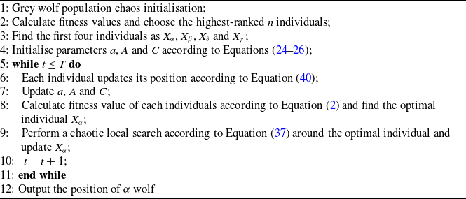
The chaos grey wolf optimiser pseudo-code is shown below in algorithm 1.
CGWO algorithm

4.0 Algorithm performance testing
4.1 Benchmark function
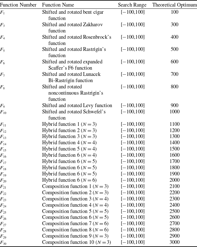
In this section, we comprehensively tested the overall performance of the CGWO algorithm by using the internationally widely recognised CEC2017 test set [Reference Wu, Mallipeddi and Suganthan27]. The CEC2017 benchmark test set comprises 29 evaluation functions, and the specific information is shown in Table 1. Where
 ${F_1}$
and
 ${F_3}$
are unimodal;
 ${F_4} - {F_{10}}$
are basic multimodal;
 ${F_{11}} - {F_{20}}$
are hybrid; and
 ${F_{21}} - {F_{30}}$
are composite functions.
Detailed information of CEC2017

The CEC2017 benchmark test set validates the performance of the optimization algorithms in a number of different situations and dimensions by designing a series of challenging optimisation problems. It assesses both algorithms’ broad exploratory power and its adaptability to restrictions and intricate settings.
4.2 Parameter setting
We selected four representative algorithms to compare their performance with the CGWO, namely the PSO algorithm [Reference Kennedy and Eberhart12], the whale optimisation algorithm (WOA) [Reference Mirjalili and Lewis28], the artificial ecosystem optimisation (AEO) [Reference Zhao, Wang and Zhang29], and the GWO [Reference Mirjalili, Mirjalili and Lewis16].
PSO is a classical algorithm that guides the search process through the interaction of the global optimal solution and the local optimal solution to achieve the optimal solution of the problem; WOA mirrors the foraging patterns of humpbacks; this strategy diminishes premature convergence and boosts comprehensive exploration; AEO models organismal interactions within ecosystems, proving efficient for intricate, multi-parameter optimisation; GWO, in which the
 $\alpha $
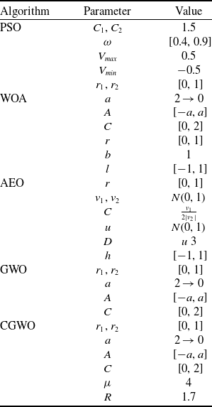
wolf guides the other wolves and eventually approaches the optimal solution, converges rapidly but easily gets trapped in local optima. Table 2 displays the configuration parameters for each algorithm; to ensure fairness, both GWO and CGWO have the same common parameter settings.
Parameter values of algorithms

To minimise total experimental error, the parameters are set uniformly throughout the experiment. Each function in the CEC2017 test set is simulated independently for all algorithms for 10 times, and each iteration is set to have a maximum number of iterations of 300, with a test dimension of 30 dimensions, while all algorithm population sizes are set to 30.
4.3 Performance analysis
This section aims to analyse the performance of CGWO and the four algorithms it compares with. It is divided into two parts. The first part analyses the quality of algorithm optimisation by running the above algorithms on the CEC2017 test set and obtaining the average and standard deviation of the optimal solutions for each algorithm. The second part conducts a detailed analysis of the convergence performance of the algorithms by plotting their convergence curves in CEC2017.
4.3.1 Optimisation quality analysis
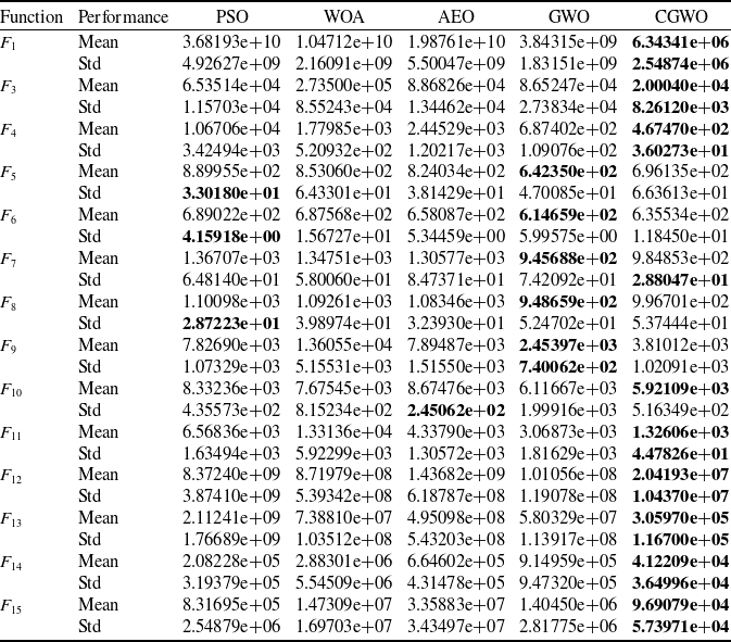
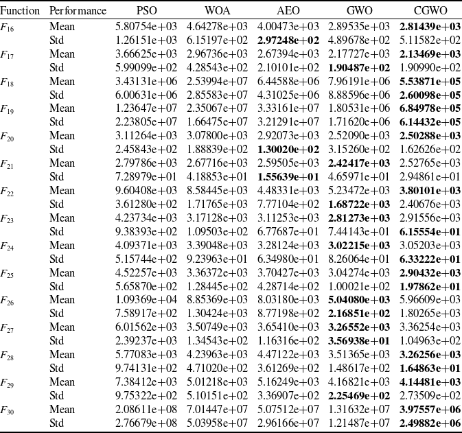
Tables 3 and 4 summarise the results of the five algorithms listed above on the CEC2017 test set. Mean refers to the average of the optimal values obtained by running each algorithms independently 10 times, and Std refers to the standard deviation of the optimal values obtained by each algorithm. The best results in the chart are displayed in bold.
CEC2017 test results (F1–F15)

Convergence performance of algorithms for different functions in CEC2017.

CEC2017 test results (F16–F30)

The experimental results in Tables 3 and 4 show that CGWO has strong versatility in optimising different types of problems. Among a total of 29 test functions, CGWO obtained results close to the theoretical optimum in 20 functions, and its results consistently ranked in the top two among all test functions, demonstrating excellent optimisation quality. In the nine test functions
 ${F_1}$
,
 ${F_4}$
,
 ${F_{12}}$
,
 ${F_{13}}$
,
 ${F_{14}}$
,
 ${F_{15}}$
,
 ${F_{18}}$
,
 ${F_{19}}$
and
 ${F_{30}}$
, the solution accuracy of CGWO is significantly higher than that of other algorithms, with an average difference of one order of magnitude. In particular, for
 ${F_1}$
and
 ${F_{13}}$
, the average value of the optimal solution obtained by CGWO is three orders of magnitude smaller than that of other algorithms. For the aforementioned nine test functions, CGWO achieves the smallest standard deviation after running independently 10 times. By comparing the average values and standard deviations of the optimal values across all algorithms, it can be concluded that CGWO demonstrates outstanding optimisation performance. The significant superiority of CGWO indicates that the chaotic logic mapping method proposed in this paper enhances population diversity, thereby increasing the likelihood of the algorithm finding high-quality solutions.
4.3.2 Convergence analysis
Figure 3 offers a visual depiction of algorithmic convergence on the CEC2017 benchmark test. In general, the CGWO algorithm has optimal convergence performance. At the beginning of the population iteration, CGWO converges significantly faster than other algorithms, which demonstrates the CGWO algorithm’s robust search capacity and efficient strategy. During the mid-to-late phases of the population iteration, the fitness value of CGWO is smaller than the other algorithms, demonstrating that CGWO converges earlier and identifies the global optimum more rapidly than other algorithms.
For the test functions
 ${F_1}$
,
 ${F_8}$
,
 ${F_{12}}$
,
 ${F_{13}}$
,
 ${F_{18}}$
,
 ${F_{20}}$
,
 ${F_{22}}$
and
 ${F_{30}}$
, the CGWO algorithm shows the best convergence performance and is substantially ahead of the other algorithms, discovering smaller global optima compared to alternative algorithms in 300 generations. For the test functions
 ${F_4}$
,
 ${F_7}$
,
 ${F_{11}}$
,
 ${F_{14}}$
,
 ${F_{17}}$
,
 ${F_{19}}$
,
 ${F_{25}}$
and
 ${F_{28}}$
, the CGWO algorithm does not manage to achieve a significant lead like the previous test functions, but still achieves the smallest fitness value, which also proves the advanced nature of the CGWO algorithm.
The experimental results presented in this chapter demonstrate the key role of chaotic initialisation, chaotic local search and leader dynamic reduction mechanisms in enhancing the efficiency of the GWO algorithm. It is proved that chaotic initialisation demonstrably yields a more uniformly distributed and randomised initial population, significantly enhancing the GWO algorithm’s initial search efficiency, making it more diversified and capable of global exploration; chaotic localised search prevents the issue of traditional methods being trapped in local optima due to over-reliance on the current optimal solution, and enhances search varity and acclerates convergence. The dynamic reduction of the leader provides an adaptive balance between global and local search, which improves the convergence speed and accuracy of the algorithm. The combination of the three can effectively improve the convergence performance of GWO in complex problems, avoid premature convergence and improve the overall performance.
5.0 3D Multi-uav path planning with cgwo algorithm
This section presents two drone deployment scenarios illustrating CGWO’s efficacy in practical applications.
5.1 Experimental parameters
In the experiment, the overall flight space is set to
 $100$
km
 $ \times 100$
km
 $ \times 500$
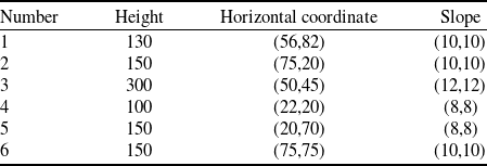
m, which includes six peaks, and the original digital terrain model is constructed according to Equation (2]. According to Reference [Reference Dan and Long30], the initial terrain model parameters are configured as follows:
 $a =\ 0.1$
,
 $b =\ 0.01$
,
 $c =\ 1$
,
 $d =\ 0.1$
,
 $e =\ 0.2$
,
 $f =\ 0.4$
and
 $g =\ 0.02$
. The peak heights, horizontal coordinates of their apexes and the slope parameters are detailed in Table 5.
Threat equivalent terrain model parameters

In the simulation test, we set the number of population to 120, the number of iterations to 300 and the number of path points between the start and end points to 10. The values of the weighting coefficients of the different cost functions in the total cost function are set:
 ${\omega _1} =\ 0.3$
,
 ${\omega _2} =\ 0.25$
,
 ${\omega _3} =\ 0.1$
,
 ${\omega _4} =\ 0.1$
,
 ${\omega _5} =\ 0.1$
and
 ${\omega _6} =\ 0.15$
. The drone’s speed is set at 40–60 m/s.
5.2 Case simulation
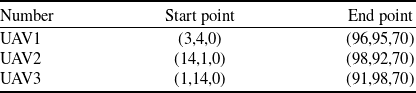
Case 1: In this case, we set up three UAVs for path planning. The starting and ending point coordinates for the three UAVs are presented in Table 6.
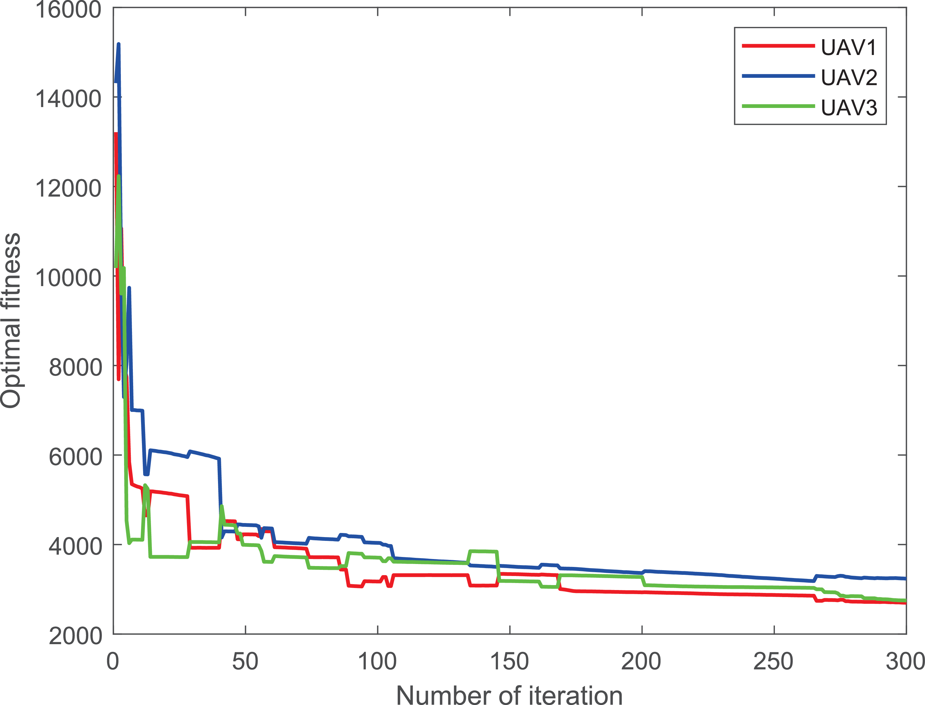
For Case 1, after 300 iterations, Figs. 4a and b represent the composite and top perspectives of the three UAVs’ path planning, respectively, demonstrating that CGWO avoids falling into a local optima; meanwhile, it is able to maintain the distances between multiple UAVs as well as the distances between the UAVs and obstacles to avoid collisions. Figure 5 represents the cost convergence trajectories of the three UAVs. It is evident that all the curves converge quickly, validating the algorithm performance.
Start and end coordinates of three drones

Three-dimensional composite and top views of Case 1.

Cost convergence curves for Case 1.

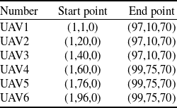
Case 2: In this case, we set up six UAVs for path planning. Table 7 lists starting and ending coordinates for the six UAVs.
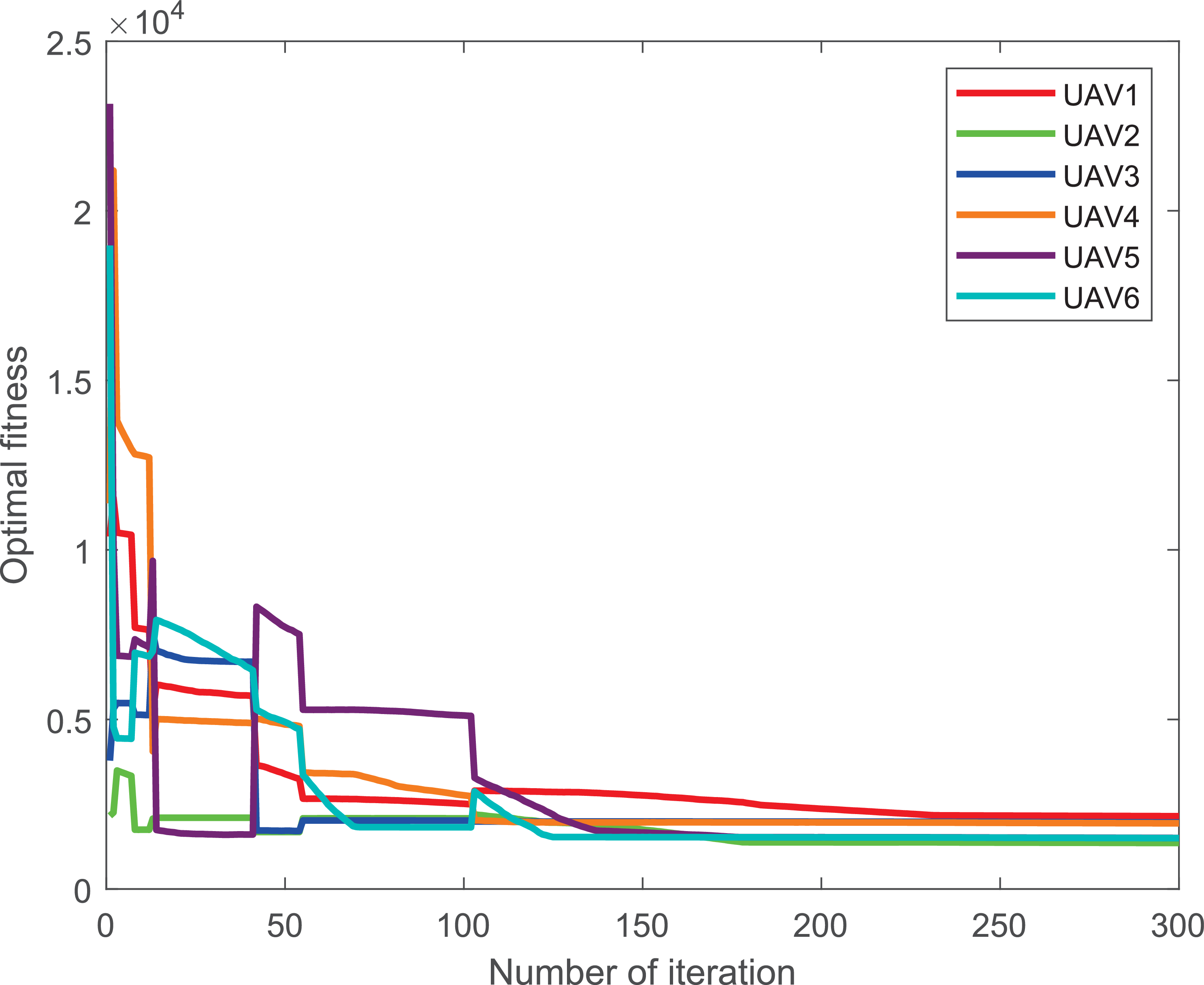
For Case 2, after 300 iterations, Figs 6a and b represent the composite and top perspectives of the six UAVs’ path planning, and according to the pictures, the distances among the six UAVs and between the UAVs and mountain peak obstacles are effectively managed, ensuring successful obstacle avoidance. Figure 7 shows the cost convergence function of the six UAVs, and all the curves converge quickly, proving the feasibility of the algorithm.
Start and end coordinates of six drones

Comparison of algorithm results

Three-dimensional composite and top views of Case 2.

5.3 Results analysis
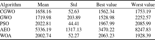
As shown in Figs 4 and 6, CGWO can generate flight trajectories that satisfy the constraints in both Case 1 and Case 2. Taking Case 1 as an example, CGWO and the other four comparison algorithms were simulated in the Case 1 scenario. Table 8 shows the average values and deviations of the cost function obtained by running the five algorithms 10 times in Case 1. CGWO obtains a mean value for the cost function that is smaller than the other four comparison functions. Although CGWO does not obtain an optimal value as good as GWO, its standard deviation is much smaller than that of GWO. This further proves the superiority of the proposed algorithm over the other four algorithms.
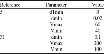
In addition, based on Case 1, the performance parameters given in reference [Reference Xu, Cao, Du and Li5, Reference Xu, Xu and Yin31] were selected to verify the superiority of the proposed algorithm. Table 9 lists the parameter values mentioned in the two references. Given the different ways in which the multi-UAV path cost functions are constructed, some of the performance parameters in this paper do not exist in these references. For performance parameters that do not exist in these references, the same performance parameter settings as in this paper are used.
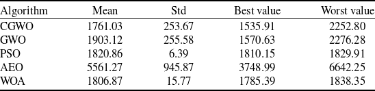
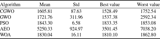
Figures 8 and 9 show the path maps obtained by simulation using the performance parameters in References [Reference Xu, Cao, Du and Li5] and [Reference Xu, Xu and Yin31] in Case 1. Tables 10 and 11 show the average values, standard deviations, optimal values and worst values of the cost function obtained by the proposed algorithm and the comparison algorithm under two different performance parameters.
Based on the path curves and computational results obtained from the performance parameters in the aforementioned applications and references, it can be concluded that CGWO can generate path curves that meet the conditions and are safe and collision-free under different performance parameter conditions, demonstrating excellent generalisation capabilities. Based on the computational results, it can be concluded that CGWO achieves the lowest average value of the cost function. Although CGWO ranks third in terms of standard deviation, its optimal performance in the average value of the cost function indicates that CGWO maintains global optimisation capabilities while also exhibiting stability and robustness. This further demonstrates that CGWO exhibits superior optimisation performance compared to the four comparison algorithms.
Performance parameters of relevant references

Cost convergence curves for Case 2.

Algorithm results of Reference [Reference Xu, Cao, Du and Li5]

Three-dimensional composite and top views of Reference [Reference Xu, Cao, Du and Li5].

Three-dimensional composite and top views of Reference [Reference Xu, Xu and Yin31].

Algorithm results of Reference [Reference Xu, Xu and Yin31]

6.0 Conclusions
In this study, we introduce a multi-UAV trajectory design approach named as CGWO, aiming to address multi-UAV system path planning challenges. The improved algorithm builds upon the GWO framework, integrating chaotic logic mapping and a leadership-based dynamic reduction strategy. Chaotic logic mapping is applied to population initialisation and local search components. Chaotic initialisation significantly enhances population diversity, effectively expanding the coverage of the search space. To address the issue of GWO easily getting stuck in local optima, chaotic local search is introduced after individual position updates. Since chaotic logic mapping possesses universality, unpredictability, and non-periodicity, it can effectively guide individuals out of local optimum traps, thereby improving the search quality of the algorithm. The leadership dynamic decay strategy dynamically adjusts the search strategy based on the progression of the iterative process. In the early stages, the focus is on global search, gradually transitioning to local search in later stages.
In the algorithm performance test, the CEC2017 test set was used as the test basis, and numerical experiments were conducted on CGWO and four commonly used algorithms. In some test functions, the average test results obtained by CGWO are two orders of magnitude or more smaller than the average test results obtained by other algorithms. According to the numerical results obtained, it can be proven that CGWO has the best convergence accuracy in more than
 $66{\rm{\% }}$
of the test functions. According to the convergence curve diagram, the convergence speed of the CGWO algorithm is superior to that of the comparison algorithms in most cases.
In simulation experiments, the CGWO algorithm was used to generate safe paths that avoid collisions between drones and between drones and obstacles, meeting mission requirements. This greatly improved the collaborative efficiency of multi-drone systems. The comparison results also show that the path cost generated by CGWO is significantly lower than that of the other four comparison algorithms, verifying the effectiveness of this algorithm in solving multi-UAV cooperative path planning problems.
Financial support
The work was supported in part by the National Natural Science Foundation of China under Grant 62573175, in part by the Natural Science Foundation of Hebei Province under Grant F2025202029, and in part by the Natural Science Foundation of Tianjin under Grant 23JCYBJC00930.