

Introduction
There is converging evidence that, although physical aggression (AGG; e.g. assaulting others, bullying) and non-aggressive rule-breaking (RB; e.g. lying, stealing, vandalism) are moderately to strongly correlated, they nevertheless constitute meaningfully distinct dimensions of antisocial behavior. As reviewed previously (Tackett et al. Reference Tackett, Krueger, Iacono and McGue2005; Tremblay, Reference Tremblay2010; Burt, Reference Burt2012), AGG and RB evidence distinctive developmental trajectories, demographic correlates, personological underpinnings, and, perhaps most importantly, etiologic differences. In particular, a meta-analysis of 103 twin and adoption studies (Burt, Reference Burt2009) revealed that AGG was a highly heritable condition (65% of the variance), with little role for the shared environment (i.e. influences that create similarity regardless of the extent of genetic similarity). By contrast, while genetic influences also contributed to RB (48%), there was an important role for shared environmental effects as well (18%).
Although such findings clearly point to substantive etiologic distinctions between AGG and RB, the identification of larger shared environmental influences on RB than on AGG in a classical twin study design does not reveal anything about the specific aspects of the environment that underlie this effect (sometimes referred to as the ‘black box’ problem). The larger environmental contributions to RB could thus be a function of the parent–child relationship, divorce, peers and/or broader contextual influences, each of which has different ramifications for our understanding of the origins of RB. It is equally unclear what specific genes may comprise and underlie the differential heritability of AGG and RB. Fortunately, a small handful of studies have begun to fill these gaps in the literature (see Raine et al. Reference Raine, Brennan and Mednick1994; Gorman-Smith et al. Reference Gorman-Smith, Tolan, Zelli and Huesmann1996; Lynam et al. Reference Lynam, Caspi, Moffitt, Wikstrom, Loeber and Novak2000; Breslau et al. Reference Breslau, Borges, Saito, Tancredi, Benjet, Hinton and Medina-Mora2011; Klahr et al. Reference Klahr, Klump and Burt2014). For example, Klahr et al. (Reference Klahr, Klump and Burt2014) examined whether maternal negativity was differentially associated with AGG and RB in a sample of 1648 child twins from 824 families. Results revealed that the association with maternal negativity was entirely environmental in origin for RB, but was both genetic and environmental in origin for AGG. Moreover, the shared environmental correlation between maternal negativity and RB was significantly larger than that with AGG (0.82 and 0.62, respectively), indicating that maternal negativity is one source of the etiologic differences between AGG and RB prior to adulthood.
For their study, Breslau et al. (Reference Breslau, Borges, Saito, Tancredi, Benjet, Hinton and Medina-Mora2011) focused on broader societal effects that may differ across AGG and RB. They specifically examined adults of Mexican ancestry in various stages of migration: (a) adults of Mexican ancestry living in the USA but who were raised in Mexico; (b) adults of Mexican ancestry who were born in the USA or who came to the USA as children; and (c) adults of Mexican ancestry born in the USA to at least one US-born parent. Comparing migrants (i.e. group a) with those born and/or raised in the new country (i.e. groups b and c) allowed researchers to examine the influence of broader societal/ environmental conditions on behavior prevalence. Results revealed that, when compared with group a, the odds ratios for AGG (0–2 v. 3+ symptoms) in groups b and c were 1.51 and 3.07, whereas those for RB were 3.45 and 10.50. Such results highlight a likely role for societal or broader contextual influences in adult RB in particular.
Although the above studies have begun to narrow in on the specific environmental experiences that underlie the stronger environmental influences on RB, much remains unknown. There is thus a clear need for additional research on the source of environmental differences between AGG and RB. Neighborhood context is an excellent candidate for such work given the vast literature tying neighborhood disadvantage to antisocial behavior across the lifespan (as two representative examples, see Gorman-Smith et al. Reference Gorman-Smith, Tolan and Henry2000; Leventhal & Brooks-Gunn, Reference Leventhal and Brooks-Gunn2000), as well as the focus on (as yet unidentified) contextual environmental influences in Breslau et al. (Reference Breslau, Borges, Saito, Tancredi, Benjet, Hinton and Medina-Mora2011). The current study thus sought to examine neighborhood disadvantage as a unique predictor of RB, evaluating whether unrelated adults residing in the same neighborhood were more similar in their RB (but not their AGG) than would be expected by chance. This design functions in some ways as a conceptual extension of studies using similarity among step-siblings to make inferences regarding the importance of the shared environment (Burt, Reference Burt2014). It is important to note, however, that neighborhood-level similarity could reflect genetic similarity between neighbors and/or common selection processes rather than an effect of the environment (Burt, Reference Burt2014). We thus attempted to evaluate the role(s) of neighborhood selection and gene–environment correlation (i.e. rGE; non-random or genetically influenced exposure to particular environmental experiences, in this case neighborhood residence) in our results. We specifically reasoned that environmentally mediated similarity among neighbors would not be present in new residents. Instead, similarity should emerge/increase after residing in the neighborhood for some time. We also restricted our analyses to neighborhoods with similar levels of likely selection characteristics, reasoning that the continued presence of neighborhood-level variance in a subsample of similar neighborhoods (which should be influenced by similar selection processes) would implicate an environmentally mediated process. Although conclusions from these analyses will not definitively establish neighborhood as an environmental predictor of RB given the pervasive nature of genetic influences on human behavior and experience, positive results would nevertheless point to neighborhood context as a predictor of RB in particular and begin to clarify whether these neighborhood-level influences on RB function at least in part via the environment.
Method
Participants
Two independent samples were collected. The first sample consisted of 1430 adults (46.7% women; 86.2% non-Hispanic Caucasian, average age of 27.9 years with a range of 18–70 years) nested in 997 census tracts across the state of Michigan. Participants were recruited via the web-based Amazon marketplace MTurk (Buhrmester et al. Reference Buhrmester, Kwang and Gosling2011). MTurk has a large (n > 100 000) and diverse ‘workforce’ of individuals who complete surveys, writing, and other such tasks on-line. For the current study, we required that all participants resided in Michigan, and paid $1.50 for completion of the assessment. The second sample consisted of 1159 adults (66.4% women; 83.7% non-Hispanic Caucasian, average age of 52.6 years with a range of 18–95 years) nested in 260 modestly to severely disadvantaged census tracts across the state of Michigan. For the latter sample, anonymous mailings were sent to up to 10 randomly chosen addresses per census tract. The response rate using this approach was 72%, of which 70% agreed to participate (for a final participation rate of 50.4%). Assessments were identical across the two samples. The research protocol was approved by the Michigan State University Institutional Review Board. All participants provided informed consent.
Measures
Aggressive and non-aggressive antisocial behavior
Participants completed the Sub-Types of Antisocial Behavior questionnaire (STAB; Burt & Donnellan, Reference Burt and Donnellan2009), which includes a 10-item AGG scale (e.g. threatened others; gotten into physical fights; α = 0.89 for sample 1 and 0.85 for sample 2) and an 11-item RB scale (e.g. shoplifted things; sold drugs; α = 0.90 for sample 1 and 0.76 for sample 2). Participants were asked to rate how often they had engaged in each behavior using a five-point scale (1 = never to 5 = nearly all the time). Items were summed.
Neighborhood structural characteristics
We administered the 13-item Extent of Neighborhood Problems scale (Tolan et al. Reference Tolan, Gorman-Smith and Henry2003) to all participants (α = 0.94 for both samples 1 and 2). This scale assesses whether participants consider graffiti, drugs, vandalism, gangs, etc., to be a problem in their neighborhood. Items were rated using a five-point scale (1 = strongly agree to 5 = strongly disagree), and were reverse-scored and summed for analysis. We also collected information on the proportion of neighborhood residents living below the poverty line in each census tract (from www.Census.gov). In sample 1, neighborhood poverty ranged from 0 to 100%, with a mean of 17.5%. In sample 2, neighborhood poverty ranged from 0 to 85%, with a mean of 23.8%.
Neighborhood social processes
Two important neighborhood social processes, social cohesion and informal social control, were also assessed (Sampson et al. Reference Sampson, Morenoff and Gannon-Rowley2002; Odgers et al. Reference Odgers, Moffitt, Tach, Sampson, Taylor, Matthews and Caspi2009). The Social Cohesion Scale consists of 30 items assessing perceptions of neighborhood support, help and trust (e.g. would neighbors intervene if a fight broke out, etc.; α = 0.95 in samples 1 and 0.96 in sample 2). Items were rated using a five-point scale (1 = strongly agree to 5 = strongly disagree), and were reverse-scored and summed for analysis. Informal social control assesses the degree to which residents perceive an expectation among community residents to undertake activities that maintain social order (e.g. what would someone in your neighborhood do if … someone is trying to sell drugs to kids?). Response options for the 29 items ranged from 1 to 4 (1 = do nothing; 2 = complain or discuss with other neighbors; 3 = talk to someone who can do something about it; 4 = do something directly). Items were recoded, such that response options 1 or 2 were coded as a 0 and response options 3 or 4 were coded as a 1, and then summed.
Possible moderators
We also examined two possible moderators of neighborhood-level variance in antisocial behavior, namely genetic relatedness between neighbors and length of residence. The first was assessed with a single item, answered yes/no: ‘I have relatives living in this community’. The second was also assessed with a single item, ‘How long have you lived in your current residence?’, with response options ranging from less than 1 year up to multiple decades.
Analyses
Because participants are nested within neighborhoods, our data have a two-level structure with the participant as the lower-level unit and the neighborhood as the upper-level unit. Predictor variables can occur at either level 1 (e.g. participant age, etc.) or level 2 (i.e. neighborhood poverty). We first computed an unconditional model to estimate the neighborhood intraclass correlation, or the extent to which neighborhood contributes to the phenotypic variance in AGG or RB. We then added a series of demographic predictors to ensure that this neighborhood variance was not a function of demographic factors that might vary across neighborhood (e.g. ethnicity). We then added a series of level-1 socio-economic and family status predictors (e.g. household income, presence of children, etc.) that could partially explain any observed neighborhood variance. As a final step, we added measures of neighborhood structural characteristics and social processes and computed the proportion of neighborhood variance in antisocial behavior explained (Snijders & Bosker, Reference Snijders and Bosker2012). In this way, we were able to evaluate whether neighborhood contributes to antisocial behavior, and whether specific neighborhood variables explain a proportion of that neighborhood-level variance. All models were fitted using restricted maximum likelihood estimation in SPSS 22 (USA).
We next attempted to evaluate the effects of genetic relatedness and neighborhood selection/rGE on our findings (as recommended in Burt, Reference Burt2014). We conducted a series of confirmatory analyses to evaluate whether the neighborhood-level variance in antisocial behavior: (1) persisted across participants with and without relatives in their neighborhood (thereby attempting to confirm that unknown genetic relationships between participants do not explain the neighborhood-level variance); (2) was absent in those who just moved into their neighborhood (as would be expected if neighborhood is exerting an environmentally mediated influence on participant behavior) and increased with increasing years of residence; and (3) persisted even when limiting analyses to structurally similar neighborhoods (since neighborhood selection processes would presumably be similar for similar types of neighborhoods). Should the neighborhood-level variance in antisocial behavior persist across confirmatory analyses 1 and 3 and only after time in confirmatory analysis 2 (as defined above), it would tentatively suggest that neighborhood may be exerting an environmental influence on residents’ behavior.
Importantly, the purpose of the above confirmatory analyses was not to confirm or refute the presence of neighborhood selection (indeed, we have no doubt that there is such selection), but rather to evaluate the extent to which this selection might account for any neighborhood-level variance. Put another way, the critical issue is whether selection contributed to/accounts for the neighborhood-level variance in RB, not whether there is selection. The latter issue is somewhat similar to that for the equal environments assumption, in which twin researchers assume that monozygotic twin pairs are no more likely to share the environmental factors that are etiologically relevant to the phenotype than are dizygotic twin pairs (Plomin et al. Reference Plomin, DeFries, Knopik and Neiderhiser2013). The key point is that of etiologic relevance – are the known differences in the treatment of monozygotic and dizygotic twin pairs etiologically relevant to the outcome at hand? The current study takes a similar approach, seeking to clarify the extent to which selection/rGE might account for any neighborhood-level variance in antisocial behavior.
Results
Nearly half of the census tracts in the second sample (45.0%; n = 117 of 260) were also present in the first sample. These overlapping census tracts contained 533 participants (n = 117 in sample 1 and 416 in sample 2), none of whom participated in both samples. Given this, along with the need to maximize our statistical power, we elected to combine samples for our analyses. To accommodate any differences across samples, however, we created a sample dummy code (−1, 1) to include as a fixed effect. Moreover, because the estimation of neighborhood-level correlations requires multiple participants per neighborhood, we omitted those participants who were the only resident of a given neighborhood in our sample (n = 640 in 640 neighborhoods). Our final sample thus consisted of 1915 participants residing in 501 neighborhoods.
Descriptive statistics
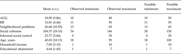
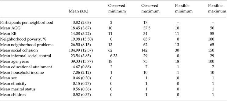
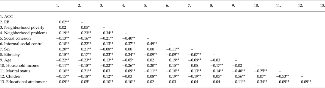
Variable means and ranges across individuals are presented in Table 1. Variable means and ranges across neighborhoods are presented in Table 2 (i.e. variables were aggregated within neighborhoods, and then descriptive statistics were based on the neighborhood aggregates). As seen there, we had sufficient variability in all variables, at both the level of the individual and the level of the neighborhood, to permit meaningful analysis. Individual-level correlations across variables are presented in Table 3. Neither AGG nor RB evidenced much of an association with neighborhood poverty. However, they were both associated with higher levels of neighborhood problems and lower levels of social cohesion and informal social control. Given that a moderate proportion of the variance in RB overlaps with that in AGG (r = 0.62; 38.4%), however, we further evaluated the extent to which these associations were specific to AGG or RB. Even when controlling for the overlap with AGG, RB remained significantly associated (p < 0.001) with all three neighborhood structural characteristic and social process variables (partial r's ranged from −0.09 to 0.16). By contrast, once we controlled for the overlap with RB, AGG was no longer associated with social cohesion or neighborhood problems (partial r's ranged from −0.04 to 0.04), although it retained a very small negative association with informal social control, (partial r was −0.06).
Individual-level descriptives (n = 1915 individuals) a

s.d., Standard deviation; AGG, physical aggression; RB, rule-breaking.
a The sample self-identified as follows: 43% male, 15% persons of color, 52% unmarried, and 59% with children. Average household income was $ 35 000 per year (coded 7.00), and ranged from less than $ 10 000 (coded 1) to more than $ 50 000 (coded 10). The average level of educational attainment corresponded to ‘some college’ (4.64), and ranged from ‘less than high school’ (coded 1) to ‘graduate degree’ (coded 7).
Neighborhood-level descriptives (n = 501 neighborhoods) a

s.d., Standard deviation; AGG, physical aggression; RB, rule-breaking.
a Mean household income by neighborhood corresponds to roughly $ 35 000 per year, and ranged from less than $ 10 000 (coded 1) to more than $ 50 000 (coded 10). The average level of educational attainment by neighborhood (4.67) corresponds to ‘some college’, and ranged from ‘some high school’ (coded 2) to ‘graduate degree’ (coded 7). To examine the proportion of participants in a given neighborhood who were male, ethnic minority, unmarried, and/or had children, those variables were each dummy coded (0, 1) for this analysis. As seen above, the average neighborhood was 46% male, 15% ethnic minority, 56% unmarried, and 52% had children. However, the full range was represented (e.g. in some neighborhoods, 0% of the participants were male, whereas in other neighborhoods, all participants were male; likewise, none of the participants had children in some neighborhoods, whereas in others, all participants did).
Individual-level correlations a

AGG, Physical aggression; RB, rule-breaking.
a Zero-order correlations were computed across the antisocial behavior, neighborhood and demographic variables. AGG and RB were log-transformed for these analyses to accommodate their non-normal distributions. Sex was coded so that −1 = women and 1 = men. Ethnicity was coded so that non-Hispanic whites were coded a −1 and persons of color were coded a 1. Marital status was coded such that −1 = married and 1 = divorced, separated or never married. Children (i.e. do you have children?) was coded so that −1 = children and 1 = no children.
Significant correlation: * p < 0.05, ** p < 0.01.
Participant demographic, socio-economic and family composition variables were also associated with antisocial behavior and neighborhood variables. AGG and RB appeared to decrease with age, and were more common in men and in persons of color. They were also associated with being divorced, separated or never married, with lower household incomes and lower educational attainment, and with never having had children. Minority status was modestly associated with being divorced, separated or never married, higher levels of neighborhood poverty, higher levels of neighborhood problems, lower household income, and lower levels of social cohesion and informal social control. Women reported higher levels of informal social control and were experiencing higher levels of neighborhood poverty than were men, but men and women did not differ in their reports of neighborhood problems or social cohesion. Finally, age was positively associated with neighborhood poverty and informal social control, but was not linked to social cohesion.
Multilevel modeling
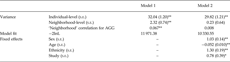
We fitted an unconditional model to AGG, followed by a model in which participant age, sex and ethnicity, and the sample dummy code were added as fixed effects. As seen in Table 4, the small amount of neighborhood-level variance found for AGG fully dissipated once we controlled for demographic factors. In short, an individual's level of AGG in adulthood appears to be largely unrelated to the neighborhood in which he or she resides.
Multi-level modeling of AGG a

AGG, Physical aggression; s.e., standard error; −2lnL, –2 log likelihood.
a Unstandardized variance component and fixed effect estimates are presented. Age was grand-mean centered. Sex and ethnicity were coded as indicated in the footnote for Table 3. We computed the proportion of neighborhood-level variance in AGG (the intraclass or ‘neighborhood’ correlation), both before (model 1) and after (model 2) controlling for level-1 demographic factors [e.g. 0.23/(29.82 + 0.23) = 0.8%].
Variance component is significant: * p < 0.05, ** p < 0.01.
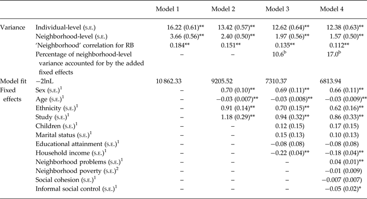
We repeated these analyses for RB. As seen in Table 5, there was significant neighborhood-level variance for RB, even when controlling for demographic, socio-economic and family composition factors. In an effort to better understand this neighborhood-level variability in RB, we added measures of the neighborhood as fixed predictors to our model. Neighborhood structural characteristics and social processes accounted for 17.0% of the neighborhood-level variance in RB. An examination of model fit statistics [–2 log likelihood (–2lnL) = 7109.86 and 6987.33, respectively] further indicated that neighborhood structural characteristics and neighborhood social processes are not redundant with one another, as the best-fitting model was that containing both types of predictor variables.
Multi-level modeling of RB a

RB, Rule-breaking; s.e., standard error; −2lnL, –2 log likelihood.
a Unstandardized variance component and fixed effect estimates are presented. Age, household income, neighborhood poverty, social cohesion, informal social control, educational attainment and neighborhood problems were grand-mean centered. Sex, ethnicity, children, divorce/separation were coded as indicated in the footnote for Table 3. We computed the proportion of neighborhood-level variance in RB (the intraclass or ‘neighborhood’ correlation), both before (model 1) and after (model 2) controlling for demographic similarities between neighbors. In model 3, we controlled for a number of potentially important individual selection factors. Model 4 added level-1 and level-2 (indicated via superscripts 1 and 2) measures of neighborhood structural characteristics and social processes as fixed effect predictors, after which we calculated the proportion of neighborhood-level variance in RB accounted for by those predictors.
b Because this proportion is calculated relative to the preceding model, we are not able to determine statistical significance.
Variance component is significant: * p < 0.05, ** p < 0.01.
Does the neighborhood-level variance in RB reflect an environmentally mediated process?
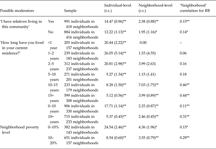
Although one could argue that the presence of neighborhood-level effects in RB, but not AGG, is inconsistent with the possibility of genetic confounds since AGG is more heritable than RB, the environmental origin of these neighborhood-level effects is as yet unknown. In an attempt to partially resolve this ambiguity, we sought to ‘rule out’ (to the extent possible) the effects of both genetic relatedness and neighborhood selection on our results via three separate sets of analyses. We first sought to confirm that our results were not a function of unknown genetic relationships between neighbors. As seen in Table 6, the neighborhood correlation was 0.15 in those with relatives living in their community and 0.14 in those without relatives living in their community. Such findings imply that unknown genetic relationships between participants do not explain neighborhood-level similarity for RB.
Confirmatory multi-level modeling of RB a

RB, Rule-breaking; s.e., standard error.
a Unstandardized variance component and fixed-effect estimates are presented. We computed the proportion of neighborhood-level variance in RB (the intraclass or ‘neighborhood’ correlation) after controlling for level-1 demographic factors (i.e. model 2 in Table 5).
Variance component is significant: * p < 0.05, ** p < 0.01 (one-tailed because we had specific hypotheses about the direction of effect).
We next attempted to clarify the role of neighborhood selection/rGE in our results. Should neighborhood-level similarity for RB reflect selection processes (in which individuals with high levels of RB preferentially assort in particular neighborhoods), we would expect neighborhood-level effects to be present within the first few years of residence. Alternatively, should neighborhood exert an environmental influence on RB, we would expect neighborhood level effects to be absent initially and to emerge over time. As seen in Table 6, there was no significant neighborhood-level variance in RB until participants had lived in their current residence for at least 10 years. However, the mean number of individuals per neighborhood was less than 2, rendering any conclusions from these data more or less meaningless. We therefore increased the n per neighborhood by splitting the sample at the 10-year mark and requiring an n of at least 2 per neighborhood. The presence of a significant neighborhood correlation in the 0- to 10-year group is consistent with some selection. However, the 95% confidence intervals do not overlap across the two groups [0–10 years: 0.11 (0.03–0.20); 10+ years: 0.31 (0.22–0.40)], which also suggests that neighborhood factors account for a greater proportion of variance in RB with increasing length of time in the neighborhood. Although this sort of cross-sectional analysis is far from conclusive, these results are at least consistent with the possibility of a partially environmentally mediated influence of neighborhood on RB.
To further clarify the role of neighborhood selection in our results, we also examined whether the neighborhood-level variance in RB persisted when restricting our analyses to structurally similar neighborhoods (since the selection processes would presumably be similar for similar types of neighborhoods). We thus grouped neighborhoods into narrow ranges of neighborhood poverty levels, focusing on the two with the largest sample sizes (i.e. <10%, n = 382 individuals in 143 neighborhoods; 10–20%, n = 651 individuals in 157 neighborhoods), and computed neighborhood correlations separately for each. As seen in Table 6, neighborhood accounted for significant variance in RB even when restricting analyses to neighborhoods that should be under similar sorts of selection pressures. Such results are consistent with a possible environmental influence of neighborhood on RB.
Confirmatory analyses
To ensure that the above results were not influenced by our decision to restrict the sample to neighborhoods with two or more participants, we repeated all of our analyses after restricting our sample to those neighborhoods with three or more participants (n = 1504 individuals in 307 neighborhoods; mean number of participants per neighborhood was 4.9 with a range of 3–17). Our conclusions were identical. Once we controlled for basic demographic variables, neighborhood-level variance was present only for RB [model 2 neighborhood r's were 0.177 for RB (p < 0.001) and 0.005 for AGG (p = 0.807)]. Structural and social characteristics of the neighborhood again accounted for neighborhood-level variance (9.9%) in RB. Moreover, the neighborhood correlation was observed in those with and without relatives in their neighborhoods (r's = 0.137 and 0.125, respectively), appeared to increase somewhat with increasing length of time in residence (r's = 0.203 and 0.290, respectively, from 0–10 and 10+ years), and persisted when examining neighborhoods that were presumably subject to similar selection processes (poverty <10% r = 0.26; poverty 10–20% r = 0.30).
Discussion
The dual goals of the current study were to constructively replicate findings of etiological distinctions between AGG and RB and to begin to identify the environmental influences unique to RB. Results revealed that although neighborhood-level influences were tiny and non-significant for AGG, they were small to moderate in magnitude for RB (11+%). Moreover, the findings for RB could not be explained by either unknown genetic relatedness across participants or neighborhood selection, and were partially attributable to structural characteristics and social processes within each neighborhood. Such results are collectively consistent with the notion that neighborhood context may account for at least a proportion of the environmental contributions unique to RB (Burt, Reference Burt2009).
The strength of the above conclusion is augmented by our large and ethnically diverse sample, as well as the representative nature of the neighborhoods under study. The average neighborhood poverty rate for the state of Michigan in 2012 was 16.3%, a proportion that is comparable with the mean level of neighborhood poverty in our final sample (19.9%). Moreover, our study focused specifically on neighborhood-level variance between many unaffiliated persons. As a result, our results are unlikely to reflect either shared informant effects or idiosyncratic informant biases. These strengths are offset, however, by our inability to definitively rule out the confounding role of possible rGE. Although our results were generally consistent with environmental origins to the neighborhood-level variance in RB (i.e. there was little evidence that our results were attributable to either genetic relatedness or neighborhood selection), this conclusion remains speculative. Relatedly, our data were cross-sectional, and thus did not allow us to examine the effects of time in the neighborhood with any certainty. Moreover, while there was some evidence of increasing similarity in RB with years in residence, this increase was seen only at the level of the neighborhood correlation. The absolute level of neighborhood-level variance was essentially unchanged across the two groups, results which may or may not be consistent with an environmentally mediated process. Longitudinal data would resolve this lingering uncertainty, as we could examine not only those who moved (allowing us to more concretely examine the possible role of selection/rGE), but also those who did not (does neighbor similarity increase with time in residence?). Future research should seek to do just this.
Next, although our sample is large and includes adults residing in disadvantaged neighborhoods, it is nevertheless unclear whether participants in our sample were representative of their neighborhoods. To preliminarily evaluate this issue, we evaluated whether census data on overall neighborhood ethnicity predicted mean neighborhood ethnicity (as reported in Table 2). Across the 501 neighborhoods examined here, census data and mean neighborhood ethnicity were correlated (r = 0.68, p < 0.001). More concretely, in 330 of the neighborhoods represented in our sample, all of our participants identified themselves as white. The census data were consistent with this: the mean proportion of white individuals in those neighborhoods was 89.0%, while the mean proportion of black individuals was 6.9%. In short, there is evidence, albeit limited, to suggest that our participants are indeed representative of their overall neighborhoods. Finally, although there are several approaches that can be taken to designate neighborhood boundaries, the current study made use of census tracts. Although census tracts represent a unit of population and geographic size that corresponds fairly well to what is commonly meant by the term neighborhood, it is nevertheless the case that census tracts and what would be socially agreed upon as neighborhoods may not coincide. This is an important measurement issue that is beyond the scope of the current study.
Despite these limitations, our study has two broad sets of implications for future research. First, and most importantly, the current results bolster prior suggestions that broader contextual experiences, like the structural and social characteristics of one's neighborhood, contribute in a meaningful way to RB during adulthood, and not to AGG (Breslau et al. Reference Breslau, Borges, Saito, Tancredi, Benjet, Hinton and Medina-Mora2011). Our results also imply that the association with RB may be environmental in origin. Neighborhood-level variance in RB persisted to those without relatives living in their community and when examining structurally similar neighborhoods, and may increase with increasing years of neighborhood residence (although this last point is less certain than the other two). Such findings collectively point to a possible environmental effect of neighborhood on RB, particularly when results are viewed alongside those of prior adoption, twin and nuclear twin-family studies (Burt, Reference Burt2009; Burt & Klump, Reference Burt and Klump2012). Regardless of the origins of their association, however, it is nevertheless the case that the unique links between neighborhood residence and RB point to the presence of substantive etiologic distinctions between aggressive and non-aggressive antisocial behavior, and underscore the advantage of differentiating between these dimensions in future research.
Second, child and family researchers have been somewhat slow to adopt the use of genetically informative designs to study the role of environmental influences, often opting for traditional family designs (i.e. family members who reside together) despite the notable absence of genetic control that characterizes such work. This is quite problematic, since positive results can be just as easily attributed to common genes as to common environmental experiences. Genetically informative designs like twin and adoption studies overcome this confounding of environmental and genetic effects to allow for stronger causal inferences. As discussed in Burt (Reference Burt2014), however, genetically informative studies could conceivably be extended beyond traditional twin and adoption designs: indeed, studies of genetically unrelated persons who share a particular environmental experience could theoretically be used to estimate the environmental contributions of that experience, provided there is appropriate attention to selection. The design employed here sought to show proof of concept for this idea, examining unrelated participants who reside in the same neighborhoods to evaluate whether neighborhood context might account for some of the previously identified environmental influences on RB. Results were encouraging, particularly when viewed alongside prior twin and adoption research (Burt, Reference Burt2009), but were nonetheless limited by our inability to rule out issues of selection and gene–environment correlation with certainty. As such, this study represents only an initial foray into the promise of such designs. Future work should seek to develop additional, stronger designs capable of more clearly leveraging genetic un-relatedness to improve causal inferences regarding the environment.
Acknowledgements
This project was supported by R01-HD066040 from the Eunice Kennedy Shriver National Institute for Child Health and Human Development (NICHD). The content is solely the responsibility of the authors and does not necessarily represent the official views of the NICHD or the National Institutes of Health. The authors thank all participants for making this work possible.
Declaration of Interest
None.