1 Introduction
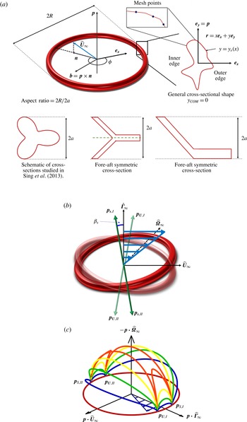
Most particles tumble continuously in a Newtonian fluid subject to a simple shear flow at low Reynolds number because they respond more strongly to the vorticity than to the extensional component of the flow (Bretherton Reference Bretherton1962). However, rings with certain cross-sectional shapes, as shown in figure 1(a), are shown to exhibit permanent alignment at finite particle aspect ratios (Singh, Koch & Stroock Reference Singh, Koch and Stroock2013). The aspect ratio (
 $A=R/a$
) is defined as the ratio of the maximum extent of the particle in the plane of the ring (
 $2R$
) and the maximum extent of the particle along the axis of symmetry (
 $2a$
) as shown in figure 1(a). This finding is fascinating as the dynamics of the particle is not only affected by the particle shape on the larger length scale, but is significantly influenced by the geometry of the smaller dimension to the point that it can lead to a bifurcation in the dynamics. In this paper, we describe the mechanism leading to alignment of rings with certain cross-sections. Using this mechanism, we obtain cross-sectional geometries that allow rings to align at much smaller aspect ratios (
 ${<}10$
) than the previously reported minimum of 30 (Singh et al.
Reference Singh, Koch and Stroock2013). This is important from the standpoint of fabrication as a higher aspect-ratio ring will be more prone to bending, buckling and breakage and thus, might not align. We also elucidate the mechanism that leads to cross-stream migration of particles that lack fore–aft or mirror symmetry. We show ways to control the magnitude of this migration or drift velocity by appropriate choice of the cross-sectional geometry. We point out that this ability to control dynamics of individual particles could allow for precise control over the macroscopic properties of the suspension.
Ring-shaped particles that align in a simple shear flow. (a) Schematic of a ring with a non-circular cross-section that is representative of the geometry studied here. The cross-sections on the left and in the centre have mirror or fore–aft symmetry about a plane normal to
 $\boldsymbol{p}$
. An orthogonal coordinate system defined by the axis of symmetry (
 $\boldsymbol{p}$
), the projection of the flow direction (
 $\hat{\boldsymbol{U}}_{\infty }$
) in the plane of the ring (
 $\boldsymbol{n}$
) and a vector
 $\boldsymbol{b}=\boldsymbol{p}\times \boldsymbol{n}$
. The centre of this coordinate system is chosen such that the centre of mass of the particle lies at the origin
 $\boldsymbol{r}_{\mathit{COM}}\boldsymbol{\cdot }\boldsymbol{p}=0$
. The azimuthal angle (
 $\unicode[STIX]{x1D719}$
) is defined relative to
 $\boldsymbol{n}$
. The inset also shows the one-dimensional (1-D) mesh and a 2-D coordinate system (
 $x,y$
) with the origin at the centre of mass (COM) of the particle.
 $\boldsymbol{e}_{\boldsymbol{x}}$
is a unit radial vector in the plane perpendicular to
 $\boldsymbol{p}$
while
 $\boldsymbol{e}_{\boldsymbol{y}}$
is a unit vector along
 $\boldsymbol{p}$
. (b) The stable fixed orientation
 $\boldsymbol{p}_{\boldsymbol{s}}$
(solid) and the unstable orientation
 $\boldsymbol{p}_{\boldsymbol{U}}$
(transparent), relative to the flow field. Both
 $\boldsymbol{p}_{\boldsymbol{s}}$
and
 $\boldsymbol{p}_{\boldsymbol{U}}$
lie in the flow–gradient plane and make an angle of
 $\unicode[STIX]{x1D6FD}_{s}$
with the gradient direction (
 $\hat{\unicode[STIX]{x1D71E}}_{\infty }$
). (c) Orientation trajectories for
 $\unicode[STIX]{x1D706}=-1.1$
. The trajectories move towards the stable nodes and away from the unstable nodes.

A simple shear flow is a good local approximation to a pressure driven flow, if the channel size is much larger than the length scale of interest, which is the particle dimension in our case. Thus, a simple shear flow could approximate processing flows such as injection moulding, extrusion and spin casting in certain regions of the flow field. Particles aligning in a simple shear flow provide unique opportunities in the material processing industry to impart enhanced properties using current processing technologies. Particles that align in a simple shear flow could be embedded in composites during curing to impart anisotropic properties to the final product. For instance, a composite material with aligned, rigid rings would have enhanced specific stiffness. Aligned particles are also more effective at reinforcing composites prone to plastic deformation (Bao, Hutchinson & McMeeking Reference Bao, Hutchinson and McMeeking1991). Aligned particles with cross-stream migration have possible application as surface modifying agents in polymer composite materials processed in mould filling flows. These particles could be systematically deposited by the flow onto a surface to improve its scratch resistance (Isla et al. Reference Isla, Brostow, Bujard, Esteves, Rodriguez, Vargas and Castano2003).
The motion of particles in a simple shear flow has been studied for over a century. Einstein (Reference Einstein1906) in his study of the effective viscosity of sheared suspensions showed that a rigid sphere rotates steadily along the fluid vorticity in an unbounded simple shear flow. Later, Jeffery (Reference Jeffery1922) demonstrated that spheroids rotate in periodic orbits in a simple shear flow slowing down but not stopping when the large dimension of the particle is nearly perpendicular to the velocity-gradient direction. Four decades later, Bretherton (Reference Bretherton1962) proved that this periodic tumbling was not restricted to spheroids but spanned almost all axisymmetric particles, except for a few shapes of extreme aspect ratio. This prediction of Bretherton about the tumbling behaviour of axisymmetric particles has been tested by both theory and experiments for discs and fibres (Trevelyan & Mason Reference Trevelyan and Mason1951; Anczurowski & Mason Reference Anczurowski and Mason1967; Stover & Cohen Reference Stover and Cohen1990). The particle tumbles in one of the infinitely many orbits depending on its initial orientation. At dilute particle concentrations, there is a distribution of particle orientations across various orbits due to secondary effects such as particle interactions or Brownian motion (Leal & Hinch Reference Leal and Hinch1971; Rahnama, Koch & Shaqfeh Reference Rahnama, Koch and Shaqfeh1995). This distribution across orbits along with particle tumbling ensures a dispersion of orientations in the suspension. An aligning particle, on the other hand, should always move towards a stable orientation irrespective of the initial orientation of the particle. Hence a sheared suspension of aligned particles should possess a micro-structure with a high degree of anisotropy.
Bretherton (Reference Bretherton1962) was the first to propose a geometry that aligned in a simple shear flow. The body was a thin rod with slightly non-spherical lobes attached at each end, such that the lobe size was much smaller than the rod length. However, he showed that the aspect ratio of the rod would need to be much larger than the exponential of the ratio of the length of the rod and the diameter of the lobes for the particle to align, leading to impractically low rigidity of the rod. Over half a century later Singh et al. (Reference Singh, Koch and Stroock2013), predicted the existence of rings with certain cross-sections that align at finite particle aspect ratios. However, the cross-sectional shapes studied in Singh et al. (Reference Singh, Koch and Stroock2013) were limited to a very specific perturbation of a circular cross-section. In this paper, we elucidate the mechanism of alignment by giving insight into the forces that lead to particle alignment in a simple shear flow. In particular, we identify ways to control rotation of a ring, by changing the cross-sectional shape.
An axisymmetric particle can also migrate in a simple shear flow if it lacks fore–aft or mirror symmetry about a plane normal to the axis of symmetry. Brenner (Reference Brenner1964) and Nir & Acrivos (Reference Nir and Acrivos1973), showed that particles that lack fore–aft symmetry can possess a cross-stream drift velocity. However, particles that tumble periodically undergo no net migration. Curved fibres can break this periodicity and lead to a constant cross-stream migration (Wang et al. Reference Wang, Tozzi, Graham and Klingenberg2012). However, such particles do not migrate for all initial orientations and the drift velocity depends on the initial orientation of the particle. Kim & Rae (Reference Kim and Rae1991) showed that screw-shaped particles migrate along or opposite to the vorticity direction depending on the handedness of the particle. However, the magnitude of the drift velocity of a screw shaped particle was shown to depend on its initial orientation. In all the above studies, the translational motion is either periodic with no net migration or the migration velocity depends on the initial particle orientation. A ring that attains an equilibrium orientation in a simple shear flow can possess a constant cross-stream velocity if it lacks fore–aft symmetry about a plane normal to the axis of symmetry of the particle. The particle obtains this constant drift velocity as it approaches the stable orientation in a time that scales with the inverse of the strain rate. We describe the mechanism leading to this drift and ways to control its magnitude by changing the cross-sectional geometry. We also elucidate the effect of the equilibrium orientation of the particle on this drift velocity.
The rotation and migration of particles in an external flow field depends on the stresses acting on the particle surface. We numerically obtain the stresses on the particle surface using the boundary element method (BEM). BEM is usually used if the primary goal is to obtain the value of the variable on the boundary. However, BEM can only be used if the fundamental solution of the governing differential equations is known (Abramowitz & Stegun Reference Abramowitz and Stegun1964). The flow field generated by a point force is a fundamental solution to the governing equations at low Reynolds number and thus we can use BEM to obtain the force per unit area exerted by the fluid on the particle surface. In our case BEM not only reduces the dimensionality of the problem, but also allows us to solve the problem in an unbounded domain.
In the following section, we solve the dynamical equations that describe the rotation of the particle and obtain the necessary conditions for alignment in a simple shear flow. In § 3 we formulate the problem and set-up the equations necessary to obtain parameters governing the motion of particles in a linear flow field. The equations are numerically solved using the boundary element method. Section 4 describes the mechanisms for alignment and cross-stream drift by visualizing the flow field and stresses acting on the particle. We suggest shapes that align at low values of aspect ratios using BEM calculations. We also elucidate the importance of particle orientation on the particle drift. Section 5 presents the conclusion and implications of the ability to control particle dynamics for manipulating macroscopic properties of particle suspensions.
2 Particle dynamics in linear flows
The linearity of Stokes flow is used to obtain the functional form of the rate of change of orientation (
 $\dot{\boldsymbol{p}}$
) as well as the drift velocity (
 $\boldsymbol{U}_{\boldsymbol{p}}$
) of an axisymmetric particle in an unbounded linear flow field.
 $\dot{\boldsymbol{p}}$
and
 $\boldsymbol{U}_{\boldsymbol{p}}$
can be described fully by three scalar parameters,
 $\unicode[STIX]{x1D706},\unicode[STIX]{x1D702}_{1}$
and
 $\unicode[STIX]{x1D702}_{2}$
, that depend on the particle geometry (Singh et al.
Reference Singh, Koch and Stroock2013). The rotation parameter,
 $\unicode[STIX]{x1D706}$
, determines the rate of change of orientation of an axisymmetric particle and depends purely on its geometry. The rate of change of orientation (
 $\dot{\boldsymbol{p}}$
) of the particle is given by
 $$\begin{eqnarray}\dot{\boldsymbol{p}}=\boldsymbol{p}\boldsymbol{\cdot }\unicode[STIX]{x1D64D}^{\infty }+\unicode[STIX]{x1D706}(\unicode[STIX]{x1D640}^{\infty }\boldsymbol{\cdot }\boldsymbol{p}-\boldsymbol{p}\boldsymbol{p}\boldsymbol{ : }\unicode[STIX]{x1D640}^{\infty }\boldsymbol{p})\end{eqnarray}$$
as shown by Jeffery (Reference Jeffery1922) and Bretherton (Reference Bretherton1962). Here
 $\boldsymbol{p}$
is the particle orientation.
 $\unicode[STIX]{x1D64D}^{\infty }$
and
 $\unicode[STIX]{x1D640}^{\infty }$
are the vorticity and straining tensor of a linear flow field respectively and are given by
 $$\begin{eqnarray}\displaystyle & \unicode[STIX]{x1D64D}^{\infty }={\textstyle \frac{1}{2}}(\unicode[STIX]{x1D735}\boldsymbol{u}^{\infty }-(\unicode[STIX]{x1D735}\boldsymbol{u}^{\infty })^{\text{T}}), & \displaystyle\end{eqnarray}$$
 $$\begin{eqnarray}\displaystyle & \unicode[STIX]{x1D640}^{\infty }={\textstyle \frac{1}{2}}(\unicode[STIX]{x1D735}\boldsymbol{u}^{\infty }+(\unicode[STIX]{x1D735}\boldsymbol{u}^{\infty })^{\text{T}}), & \displaystyle\end{eqnarray}$$
 $\boldsymbol{u}^{\infty }$
is the fluid velocity in the absence of the particle. The migration parameters
 $\unicode[STIX]{x1D702}_{1}$
and
 $\unicode[STIX]{x1D702}_{2}$
determine the drift velocity of the particle relative to the fluid velocity at its centre of mass (COM) which takes the form given by
 $$\begin{eqnarray}\boldsymbol{U}_{\boldsymbol{p}}=\boldsymbol{u}^{\infty }(\boldsymbol{r}_{\mathit{COM}})+\unicode[STIX]{x1D702}_{1}\unicode[STIX]{x1D640}^{\infty }\boldsymbol{\cdot }\boldsymbol{p}+\unicode[STIX]{x1D702}_{2}(\,\boldsymbol{p}\boldsymbol{p}\boldsymbol{p}\boldsymbol{ : }\unicode[STIX]{x1D640}^{\infty }).\end{eqnarray}$$
Equation (2.3) indicates that a particle with mirror or fore–aft symmetry about a plane normal to
 $\boldsymbol{p}$
, as shown in figure 1(a), will not drift as orientation
 $\boldsymbol{p}$
and
 $-\boldsymbol{p}$
are equivalent. As per (2.3), this is true only when
 $\unicode[STIX]{x1D702}_{1}=\unicode[STIX]{x1D702}_{2}=0$
. Absence of fore–aft symmetry is the necessary condition for having a finite cross-stream drift. In this section we obtain the necessary conditions for particle alignment and obtain this orientation in terms of the rotation parameter,
 $\unicode[STIX]{x1D706}$
.
We use the orthogonal coordinate system, as shown in figure 1(b), defined by the flow (
 $\hat{\boldsymbol{U}}_{\infty }$
), the gradient (
 $\hat{\unicode[STIX]{x1D71E}}_{\infty }$
) and the negative of the vorticity (
 $-\hat{\unicode[STIX]{x1D734}}_{\infty }$
) direction of a simple shear flow. Equation (2.1) can have six nodes for a general axisymmetric shape in a simple shear flow. There are two saddle nodes, independent of geometry, that correspond to rotation of the particle about its axis of symmetry, wherein
 $\boldsymbol{p}\boldsymbol{\cdot }\hat{\unicode[STIX]{x1D734}}_{\infty }=\pm 1$
. Four other nodes, two stable (
 $\boldsymbol{p}_{\boldsymbol{s}}$
) and two unstable (
 $\boldsymbol{p}_{\boldsymbol{U}}$
), can exist in the system for geometries that have
 $|\unicode[STIX]{x1D706}|>1$
. These nodes are shown in figure 1(b) for a ring-shaped particle with
 $\unicode[STIX]{x1D706}<-1$
. All four nodes lie in the flow–gradient plane and subtend an angle of
 $\unicode[STIX]{x1D6FD}_{s}=0.5\text{acos}(-1/\unicode[STIX]{x1D706})$
with the gradient direction as shown in figure 1(b). These nodes are mathematically given by
 $\boldsymbol{p}\boldsymbol{\cdot }\hat{\boldsymbol{U}}_{\infty }=\pm \!\sin ((-1/2)\text{acos}(-1/\unicode[STIX]{x1D706}))$
,
 $\boldsymbol{p}\boldsymbol{\cdot }\hat{\unicode[STIX]{x1D71E}}_{\infty }=\pm \!\cos ((1/2)\text{acos}(-1/\unicode[STIX]{x1D706}))$
and
 $\boldsymbol{p}\boldsymbol{\cdot }\hat{\unicode[STIX]{x1D734}}_{\infty }=0$
with
 $\boldsymbol{p}\boldsymbol{p}\boldsymbol{ : }\unicode[STIX]{x1D640}^{\infty }<0$
corresponding to the stable nodes, and
 $\boldsymbol{p}\boldsymbol{p}\boldsymbol{ : }\unicode[STIX]{x1D640}^{\infty }>0$
corresponding to the unstable nodes. When the particle is aligned in the gradient direction (
 $\boldsymbol{p}=\hat{\unicode[STIX]{x1D71E}}_{\infty }$
) the rate of rotation due to the straining component (
 $\unicode[STIX]{x1D706}\,\boldsymbol{p}\boldsymbol{\cdot }\unicode[STIX]{x1D640}^{\infty }$
) is higher than the rate of rotation due to the rotational component (
 $\boldsymbol{p}\boldsymbol{\cdot }\unicode[STIX]{x1D64D}^{\infty }$
) for
 $|\unicode[STIX]{x1D706}|>1$
as per (2.1). When the plane of the ring lies in the extensional quadrant these two rotation rates can be equal since the magnitude of rotation due to the straining flow is reduced. The plane of the ring being in this orientation corresponds to the stable nodes and is mathematically given by
 $\boldsymbol{p}\boldsymbol{p}\boldsymbol{ : }\unicode[STIX]{x1D640}^{\infty }<0$
.
Thus,
 $|\unicode[STIX]{x1D706}|>1$
is the only requirement for an axisymmetric particle to attain an equilibrium orientation in a simple shear flow. However, the dependence of
 $\unicode[STIX]{x1D706}$
on the geometry of the particle is non-trivial (Bretherton Reference Bretherton1962). Most axisymmetric particles, such as spheres, spheroids and cylinders, have
 $|\unicode[STIX]{x1D706}|<1$
and thus constantly tumble in a low Reynolds number simple shear flow (Bretherton Reference Bretherton1962). The rod-shaped particle with non-spherical lobes envisioned by Bretherton (Reference Bretherton1962) had
 $\unicode[STIX]{x1D706}>1$
, but the aspect ratio of the rod was impractically large. A ring-shaped particle with a specified non-circular cross-section was shown to have
 $\unicode[STIX]{x1D706}<-1$
at finite aspect ratios (Singh et al.
Reference Singh, Koch and Stroock2013). The trajectories obtained from (2.1) for
 $\unicode[STIX]{x1D706}<-1$
, as shown in figure 1(c), have some resemblance to periodic orbits far from the nodes (Jeffery Reference Jeffery1922). The four nodes in the system are an additional feature for aligning particles that emerge for shapes with
 $|\unicode[STIX]{x1D706}|>1$
. The particle orientation diverges away from the unstable nodes (
 $\boldsymbol{p}_{\boldsymbol{U}}$
) and converges towards the stable nodes (
 $\boldsymbol{p}_{\boldsymbol{S}}$
). The particle approaches a stable node in a time that scales with the inverse of the shear rate for any initial orientation. In the following section, we formulate an approach for obtaining the three dynamical parameters, namely,
 $\unicode[STIX]{x1D706},\unicode[STIX]{x1D702}_{1}$
and
 $\unicode[STIX]{x1D702}_{2}$
, for any general axisymmetric particle.
3 Computational approach
We use the solution to the governing equations of fluid flow around a particle in an unbounded domain along with the appropriate boundary conditions to derive the dynamical parameters (
 $\unicode[STIX]{x1D706},\unicode[STIX]{x1D702}_{1},\unicode[STIX]{x1D702}_{2}$
) of the particle. The boundary element method provides an elegant way of obtaining the stresses acting on the particle surface in an unbounded domain by reducing the dimensionality of the problem. A two-dimensional integral version of the creeping-flow equation is solved instead of a three-dimensional spatial partial differential equation (Youngren & Acrivos Reference Youngren and Acrivos1975; Kim & Karilla Reference Kim and Karilla1991). The integral representation of the flow around a rigid body used in this study is given by
 $$\begin{eqnarray}\boldsymbol{u}(\boldsymbol{r})=\boldsymbol{u}^{\infty }(\boldsymbol{r})+\frac{1}{8\unicode[STIX]{x03C0}\unicode[STIX]{x1D707}}\int \boldsymbol{J}(\boldsymbol{r}-\boldsymbol{r}^{\prime })\boldsymbol{\cdot }\boldsymbol{f}(\boldsymbol{r}^{\prime })\,\text{d}A^{\prime },\end{eqnarray}$$
where
 $\boldsymbol{r}$
is the position vector,
 $\boldsymbol{u}$
is the velocity of the fluid at the location
 $\boldsymbol{r}$
,
 $\boldsymbol{u}^{\infty }$
is the velocity of the imposed flow field at
 $\boldsymbol{r}$
,
 $\unicode[STIX]{x1D707}$
is the fluid viscosity,
 $\boldsymbol{f}$
is the unknown force per unit area the particle exerts on the fluid,
 $\text{d}A^{\prime }$
is the elemental area on the particle surface and
 $\boldsymbol{J}$
is the Green’s function for the creeping-flow equations. The Green’s function
 $\boldsymbol{J}$
is given by
 $$\begin{eqnarray}\boldsymbol{J}=\frac{\boldsymbol{I}}{r}+\frac{\boldsymbol{r}\boldsymbol{r}}{r^{3}}.\end{eqnarray}$$
The axisymmetry of the particle accompanied by linearity of the governing equations allows a further reduction in dimensionality of the problem if the imposed flow is linear. The linear imposed fluid velocity (
 $\boldsymbol{u}^{\infty }$
) can be defined as
 $$\begin{eqnarray}\boldsymbol{u}^{\infty }=\boldsymbol{u}_{\boldsymbol{ 0}}+\boldsymbol{r}\boldsymbol{\cdot }(\unicode[STIX]{x1D640}^{\infty }+\unicode[STIX]{x1D64D}^{\infty }),\end{eqnarray}$$
where
 $\boldsymbol{u}_{\mathbf{0}}$
is the velocity of the imposed flow at the centre of mass of the particle (
 $\boldsymbol{r}=0$
).
 $\unicode[STIX]{x1D640}^{\infty }$
and
 $\unicode[STIX]{x1D64D}^{\infty }$
represent the straining and vorticity tensor, respectively, defined in (2.2). The force per unit area (
 $\boldsymbol{f}$
) at position
 $\boldsymbol{r}$
can depend on
 $\boldsymbol{r}$
,
 $\boldsymbol{u}_{\mathbf{0}}$
,
 $\unicode[STIX]{x1D640}^{\infty }$
,
 $\unicode[STIX]{x1D64D}^{\infty }$
and the boundary conditions on the particle surface. The boundary conditions are given in terms of the linear velocity of the particle at its centre of mass (
 $\boldsymbol{U}_{\boldsymbol{p}}$
) and the angular velocity (
 $\unicode[STIX]{x1D74E}_{\boldsymbol{p}}$
) of the particle. Solid body translation (
 $\boldsymbol{u}^{\infty }=\boldsymbol{u}_{\mathbf{0}}$
) and rotation (
 $\boldsymbol{u}^{\infty }=\unicode[STIX]{x1D750}\boldsymbol{ : }\unicode[STIX]{x1D64D}^{\infty }$
) of the particle and the fluid, where
 $\unicode[STIX]{x1D750}$
is the permutation tensor, do not lead to any stress on the particle and thus the choice of origin does not affect
 $\boldsymbol{f}$
. The origin is chosen as the centre of mass of the particle without loss of generality. The position on the particle surface (
 $\boldsymbol{r}=\boldsymbol{r}_{\boldsymbol{s}}$
) can be decomposed into a component along the axis of symmetry and a component in the plane of the ring, which is given by
 $$\begin{eqnarray}\boldsymbol{r}=(\boldsymbol{r}\boldsymbol{\cdot }\boldsymbol{p})\boldsymbol{p}+\boldsymbol{r}\boldsymbol{\cdot }(\boldsymbol{I}-\boldsymbol{p}\boldsymbol{p}).\end{eqnarray}$$
The azimuthal dependence comes only from the second term in (3.3). The vector
 $\boldsymbol{e}_{\boldsymbol{x}}$
is defined normal to
 $\boldsymbol{p}$
at each azimuthal location. The projection of
 $\boldsymbol{r}$
along
 $\boldsymbol{e}_{\boldsymbol{x}}$
is represented as
 $\boldsymbol{r}_{\boldsymbol{x}}=\boldsymbol{r}\boldsymbol{\cdot }\boldsymbol{e}_{\boldsymbol{x}}\boldsymbol{e}_{\boldsymbol{x}}=\boldsymbol{r}\boldsymbol{\cdot }(\boldsymbol{I}-\boldsymbol{p}\boldsymbol{p})$
. Using these observations and the constraint that the force per unit area (
 $\boldsymbol{f}$
) must be a real vector, one can deduce that
 $\boldsymbol{f}$
must be linear in the relative translational velocity
 $\boldsymbol{U}=\boldsymbol{U}_{\boldsymbol{p}}-\boldsymbol{u}^{\infty }(\boldsymbol{r}_{\mathit{COM}})$
of the particle and the fluid, the relative rotation rate
 $\unicode[STIX]{x1D74E}=\unicode[STIX]{x1D74E}_{\boldsymbol{p}}-\unicode[STIX]{x1D750}\boldsymbol{ : }\unicode[STIX]{x1D64D}^{\infty }$
of the particle and fluid and the rate of strain
 $\unicode[STIX]{x1D640}^{\infty }$
of the fluid. The azimuthal variation of force per unit area (
 $\boldsymbol{f}$
) is thus given by
 $$\begin{eqnarray}\displaystyle \boldsymbol{f} & = & \displaystyle C_{1}\boldsymbol{U}+C_{2}\,\boldsymbol{p}\boldsymbol{p}\boldsymbol{\cdot }\boldsymbol{U}+C_{3}\boldsymbol{r}_{\boldsymbol{x}}\boldsymbol{r}_{\boldsymbol{x}}\boldsymbol{\cdot }\boldsymbol{U}+C_{4}\boldsymbol{r}_{\boldsymbol{x}}\,\boldsymbol{p}\boldsymbol{\cdot }\boldsymbol{U}+C_{5}\,\boldsymbol{p}\boldsymbol{r}_{\boldsymbol{x}}\boldsymbol{\cdot }\boldsymbol{U}+C_{6}(\boldsymbol{r}_{\boldsymbol{x}}\times \boldsymbol{p})(\boldsymbol{r}_{\boldsymbol{x}}\times \boldsymbol{p})\boldsymbol{\cdot }\boldsymbol{U}\nonumber\\ \displaystyle & & \displaystyle +\,C_{7}\unicode[STIX]{x1D74E}\times \boldsymbol{p}+C_{8}\unicode[STIX]{x1D74E}\times \boldsymbol{r}_{\boldsymbol{x}}+C_{9}(\boldsymbol{r}_{\boldsymbol{x}}\times \boldsymbol{p})\boldsymbol{r}_{\boldsymbol{x}}\boldsymbol{\cdot }\unicode[STIX]{x1D74E}+C_{10}(\boldsymbol{r}_{\boldsymbol{x}}\times \boldsymbol{p})\boldsymbol{p}\boldsymbol{\cdot }\unicode[STIX]{x1D74E}\nonumber\\ \displaystyle & & \displaystyle +\,(C_{11}(\unicode[STIX]{x1D74E}\times \boldsymbol{p})+C_{12}(\unicode[STIX]{x1D74E}\times \boldsymbol{r}_{\boldsymbol{x}}))\times (\boldsymbol{r}_{\boldsymbol{x}}\times \boldsymbol{p})+C_{13}(\unicode[STIX]{x1D74E}\times \boldsymbol{r}_{\boldsymbol{x}})\boldsymbol{\cdot }\boldsymbol{p}\boldsymbol{p}+C_{14}(\unicode[STIX]{x1D74E}\times \boldsymbol{p})\boldsymbol{\cdot }\boldsymbol{r}_{\boldsymbol{x}}\,\boldsymbol{p}\nonumber\\ \displaystyle & & \displaystyle +\,C_{15}(\unicode[STIX]{x1D74E}\times \boldsymbol{r}_{\boldsymbol{x}})\boldsymbol{\cdot }\boldsymbol{p}\boldsymbol{r}_{\boldsymbol{x}}+C_{16}(\unicode[STIX]{x1D74E}\times \boldsymbol{p})\boldsymbol{\cdot }\boldsymbol{r}_{\boldsymbol{x}}\boldsymbol{r}_{\boldsymbol{x}}+C_{17}\,\boldsymbol{p}\boldsymbol{p}\boldsymbol{p}\boldsymbol{ : }\unicode[STIX]{x1D640}^{\infty }+C_{18}\,\boldsymbol{p}\boldsymbol{r}_{\boldsymbol{x}}\,\boldsymbol{p}\boldsymbol{ : }\unicode[STIX]{x1D640}^{\infty }\nonumber\\ \displaystyle & & \displaystyle +\,C_{19}\,\boldsymbol{p}\boldsymbol{r}_{\boldsymbol{x}}\boldsymbol{r}_{\boldsymbol{x}}\boldsymbol{ : }\unicode[STIX]{x1D640}^{\infty }+C_{20}\,\boldsymbol{p}\boldsymbol{\cdot }\unicode[STIX]{x1D640}^{\infty }+C_{21}\boldsymbol{r}_{\boldsymbol{x}}\boldsymbol{p}\boldsymbol{p}\boldsymbol{ : }\unicode[STIX]{x1D640}^{\infty }+C_{22}\boldsymbol{r}_{\boldsymbol{x}}\boldsymbol{r}_{\boldsymbol{x}}\boldsymbol{p}\boldsymbol{ : }\unicode[STIX]{x1D640}^{\infty }+C_{23}\boldsymbol{r}_{\boldsymbol{x}}\boldsymbol{r}_{\boldsymbol{x}}\boldsymbol{r}_{\boldsymbol{x}}\boldsymbol{ : }\unicode[STIX]{x1D640}^{\infty }\nonumber\\ \displaystyle & & \displaystyle +\,C_{24}\boldsymbol{r}_{\boldsymbol{x}}\boldsymbol{\cdot }\unicode[STIX]{x1D640}^{\infty }+C_{25}\,\boldsymbol{p}(\boldsymbol{r}_{\boldsymbol{x}}\times \boldsymbol{p})\boldsymbol{ : }\unicode[STIX]{x1D640}^{\infty }(\boldsymbol{r}_{\boldsymbol{x}}\times \boldsymbol{p})+C_{26}\boldsymbol{r}_{\boldsymbol{x}}(\boldsymbol{r}_{\boldsymbol{x}}\times \boldsymbol{p})\boldsymbol{ : }\unicode[STIX]{x1D640}^{\infty }(\boldsymbol{r}_{\boldsymbol{x}}\times \boldsymbol{p})\nonumber\\ \displaystyle & & \displaystyle +\,C_{27}(\boldsymbol{r}_{\boldsymbol{x}}\times \boldsymbol{p})(\boldsymbol{r}_{\boldsymbol{x}}\times \boldsymbol{p})\boldsymbol{ : }\unicode[STIX]{x1D640}^{\infty }\boldsymbol{p}+C_{28}(\boldsymbol{r}_{\boldsymbol{x}}\times \boldsymbol{p})(\boldsymbol{r}_{\boldsymbol{x}}\times \boldsymbol{p})\boldsymbol{ : }\unicode[STIX]{x1D640}^{\infty }\boldsymbol{r}_{\boldsymbol{x}},\end{eqnarray}$$
where
 $C_{1},C_{2},\ldots ,C_{28}$
are independent of the azimuthal position and thus only depend on the cross-sectional shape of the axisymmetric body and the position on the cross-sectional contour. The reference for the azimuthal angle (
 $\unicode[STIX]{x1D719}$
) can be chosen relative to the line of intersection of a plane normal to
 $\boldsymbol{p}$
and the plane of the imposed linear flow. This line of intersection is along
 $\boldsymbol{n}$
as shown in figure 1(a) for a simple shear flow. Equation (3.4), which is applicable to a general linear flow field, can be used to obtain the variation of
 $\boldsymbol{f}$
with
 $\unicode[STIX]{x1D719}$
in the case of a simple shear flow. Using (3.4), equation (3.1a
) can be integrated along
 $\unicode[STIX]{x1D719}$
, using elliptic integrals (supplementary material available at https://doi.org/10.1017/jfm.2018.20), thus reducing the dimensionality of the problem. A one-dimensional (1-D) curved mesh, as shown in figure 1(a), is enough to obtain the force per unit area acting on the surface, instead of a 2-D surface mesh traditionally employed in a BEM formulation. For the purpose of obtaining
 $\unicode[STIX]{x1D706},\unicode[STIX]{x1D702}_{1},\unicode[STIX]{x1D702}_{2}$
, it is sufficient to solve the governing equations when the imposed flow is a simple shear flow and when
 $\boldsymbol{p}$
lies in the flow–gradient plane where
 $\boldsymbol{p}\neq \hat{\boldsymbol{U}}_{\infty }$
and
 $\boldsymbol{p}\neq \hat{\unicode[STIX]{x1D71E}}_{\infty }$
. The reference for the azimuthal angle is chosen along the projection of the flow direction in the plane of the ring (
 $\boldsymbol{n}$
) as shown in figure 1(a). Along with
 $\boldsymbol{n}$
, the orientation of the particle (
 $\boldsymbol{p}$
) and a vector
 $\boldsymbol{b}=\boldsymbol{p}\times \boldsymbol{n}$
define a coordinate system relative to the particle. In this case the dependence of
 $\boldsymbol{f}$
on the azimuthal angle (
 $\unicode[STIX]{x1D719}$
) given by
 $$\begin{eqnarray}\displaystyle & \displaystyle \boldsymbol{f}\boldsymbol{\cdot }\boldsymbol{n}=f_{0}+f_{1}\cos (\unicode[STIX]{x1D719})+f_{2}\cos (2\unicode[STIX]{x1D719})+f_{3}\cos (3\unicode[STIX]{x1D719}), & \displaystyle\end{eqnarray}$$
 $$\begin{eqnarray}\displaystyle & \displaystyle \boldsymbol{f}\boldsymbol{\cdot }\boldsymbol{p}=f_{4}+f_{5}\cos (\unicode[STIX]{x1D719})+f_{6}\cos (2\unicode[STIX]{x1D719}), & \displaystyle\end{eqnarray}$$
 $$\begin{eqnarray}\displaystyle & \displaystyle \boldsymbol{f}\boldsymbol{\cdot }\boldsymbol{b}=f_{7}\sin (\unicode[STIX]{x1D719})+f_{8}\sin (2\unicode[STIX]{x1D719})+f_{9}\sin (3\unicode[STIX]{x1D719}), & \displaystyle\end{eqnarray}$$
 $[f_{0},f_{1},\ldots ,f_{9}]$
, depend on the contour of the ring cross-section, size of the ring (
 $R$
) and the position on the ring cross-sectional contour. The integral in (3.1a
) in the azimuthal direction can be performed analytically using
 $\boldsymbol{f}$
as given in (3.5). The remainder of the integral is evaluated numerically by discretizing the cross-sectional contour into a mesh of
 $N$
elements as shown in figure 1(a). The left-hand side of (3.1a
), which is the fluid velocity on the ring surface, is known in terms of the linear and angular velocity of the particle at each of the
 $N$
mesh points. Thus, we obtain 3 equations at each mesh point on the cross-section for a given
 $\unicode[STIX]{x1D719}$
giving a total of
 $3N$
equations for each value of
 $\unicode[STIX]{x1D719}$
. We can obtain more equations by choosing a different value of
 $\unicode[STIX]{x1D719}$
. For this study, we need to evaluate (3.1a
) at four different values of
 $\unicode[STIX]{x1D719}$
so we have
 $10N$
equations to obtain
 $[f_{0},f_{1},\ldots ,f_{9}]$
at each of the
 $N$
mesh points. If the linear and angular velocities of the particles are also unknown, then an appropriate condition specifying the total force and torque on the body can be applied to obtain 6 additional equations. This procedure along with the detailed expression can be found in the supplementary material. The cross-sectional contour is given by
 $y_{s}=y(x)$
, where
 $x$
is the normal distance from axis of symmetry,
 $y$
is the distance along the axis of symmetry and the subscript
 $s$
represents the respective values on the cross-sectional boundary. In this analysis, the reference for the position along the axis of symmetry is chosen such that the plane of the ring,
 $y=0$
, passes through the centre of mass of the particle. This choice does not affect the value for the cross-stream drift velocity (
 $U_{d}$
). The following problems are solved using the boundary element method.
Mobility problem: The particle velocities (
 $\boldsymbol{U}_{\boldsymbol{p}}$
and
 $\unicode[STIX]{x1D74E}_{\boldsymbol{p}}$
), and thus the dynamical parameters (
 $\unicode[STIX]{x1D706},\unicode[STIX]{x1D702}_{1}$
and
 $\unicode[STIX]{x1D702}_{2}$
), are obtained by applying the force- and torque-free conditions about the COM of the particle ((3.6) and (3.7)), when the particle is oriented in the flow–gradient plane such that
 $\boldsymbol{p}\neq \hat{\boldsymbol{U}}_{\infty }$
and
 $\boldsymbol{p}\neq \hat{\unicode[STIX]{x1D71E}}_{\infty }$
.
 $$\begin{eqnarray}\displaystyle & \displaystyle \int \boldsymbol{f}(\boldsymbol{r}^{\prime })\,\text{d}A^{\prime }=\mathbf{0}, & \displaystyle\end{eqnarray}$$
 $$\begin{eqnarray}\displaystyle & \displaystyle \int \boldsymbol{r}^{\prime }\times \boldsymbol{f}(\boldsymbol{r}^{\prime })\,\text{d}A^{\prime }=\mathbf{0}. & \displaystyle\end{eqnarray}$$
Resistivity problem for alignment mechanism: The direction of the torque exerted by the fluid on the particle when it is kept stationary (
 $\boldsymbol{U}_{\boldsymbol{p}}=0$
,
 $\unicode[STIX]{x1D74E}_{\boldsymbol{p}}=0$
) with
 $\boldsymbol{p}=\hat{\unicode[STIX]{x1D71E}}_{\infty }$
distinguishes between tumbling and aligning behaviour. If the fluid applies a torque against the vorticity direction, then the particle is trying to rotate in the counter-vorticity direction towards the stable node as shown in figure 1(b). A fluid torque along the vorticity direction implies a tumbling behaviour. This resistivity problem is used to understand the alignment mechanism through visualization of stresses on the particle surface. It also gives insight into the cross-sectional geometry necessary for alignment.
Resistivity problem for drifting mechanism: The scaling for cross-stream drift of the particle (
 $\boldsymbol{U}_{d}$
) can be obtained when the particle is oriented along the stable orientation (
 $\boldsymbol{p}=\boldsymbol{p}_{\boldsymbol{s}}$
) and held stationary (
 $\boldsymbol{U}_{\boldsymbol{p}}=0$
,
 $\unicode[STIX]{x1D74E}_{\boldsymbol{p}}=0$
). At this orientation, the force acting on the particle drives its drifting motion. This problem will only be solved as a thought experiment to predict the scaling for the drift velocity, which can be obtained by equating this force to the force required for translating the particle in a quiescent fluid.
In this study, we try to understand the mechanism leading to alignment of particles at much lower aspect ratios than the previously reported minimum of 30 (Singh et al.
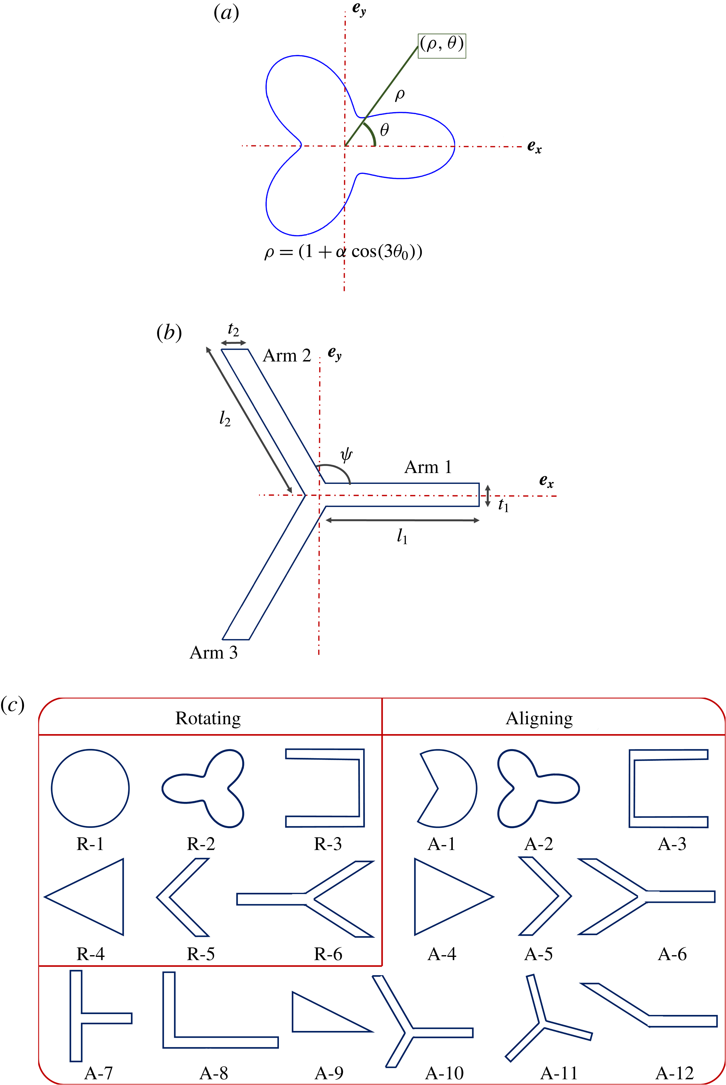
Reference Singh, Koch and Stroock2013). A family of 2-D contours is chosen based on previous insight into aligning shapes. The family of shapes given by
 $\unicode[STIX]{x1D70C}=(1+\unicode[STIX]{x1D6FC}\cos (3\unicode[STIX]{x1D703}))$
was shown to achieve permanent alignment at finite aspect ratios (Singh et al.
Reference Singh, Koch and Stroock2013). Here
 $\unicode[STIX]{x1D70C}$
and
 $\unicode[STIX]{x1D703}$
represent the polar coordinates in the plane of the cross-section (
 $x$
–
 $y$
plane) and
 $\unicode[STIX]{x1D703}$
is measured relative to
 $\boldsymbol{e}_{\boldsymbol{x}}$
, as shown in figure 2(a).
 $\unicode[STIX]{x1D6FC}$
changes the shape of the cross-section. Based on this insight a three-lobed shape shown in figure 2(b) is used for studying fore–aft symmetric shapes. This fore–aft symmetric shape can be described by 5 parameters: ‘
 $l_{1}$
’, length of arm 1; ‘
 $t_{1}$
’, thickness of arm 1; ‘
 $l_{2}$
’, length of arm 2 and arm 3; ‘
 $t_{2}$
’, thickness of arm 2 and arm 3; and
 $\unicode[STIX]{x1D713}$
, angle made by arm 2 and arm 3 with arm 1. Although this family of ‘
 $Y$
-shaped’ cross-sections does not cover all shapes, it gives insight into particle geometries that will lead to alignment. The choice of a
 $Y$
-shaped cross-section will be motivated in the next section, where results obtained from BEM are used to describe the mechanism of alignment. Cross-sections shown in figure 2(c) were also studied, but were found to align at higher aspect ratios. Cross-sections A-8 to A-12 lack fore–aft symmetry and thus can possess cross-stream drift. We shall also discuss the mechanism leading to cross-stream drift and show ways to control the magnitude of drift by proper choice of cross-sectional shape. All cross-sections shown in the remainder of the paper are in figure 1(a), where the left side of the cross-section is the inner edge closer to the ring centre while the right side is the outer edge of the ring.
Ring cross-sectional shapes studied here. (a) Shape given by
 $\unicode[STIX]{x1D70C}=1+\unicode[STIX]{x1D6FC}\cos (3\unicode[STIX]{x1D703})$
that was shown to lead to flow aligning rings by Singh et al. (Reference Singh, Koch and Stroock2013). (b)
 $Y$
-shaped fore–aft symmetric shape inspired by (a). (c) Some of the ring cross-sections studied using BEM calculations. Rings with cross-sections
 $\text{R}\text{-}i$
, for
 $i=1,2,\ldots ,6$
, rotate in a simple shear flow, while rings with cross-sections
 $\text{A}\text{-}i$
, for
 $i=1,2,\ldots ,12$
, align in a simple shear flow at finite aspect ratios.

We also solved for flow past a two-dimensional obstacle with the same shape as the ring cross-section in a two-dimensional domain using a finite element method (FEM) solver in COMSOL. This flow field qualitatively resembles the flow field around a slender ring in the cross-sectional plane near the surface of the particle. This gives a qualitative visualization of fluid velocity and stresses near the particle surface with lower computational effort. This problem also removes the effect of the size (aspect ratio) of the particle, and isolates the effect of the cross-sectional shape on the stresses acting on the particle surface. The domain size
 $L\gg a$
, ensures that the fluid velocity near the particle is not influenced by the shape of the box. The fluid velocity varies logarithmically with radial distance,
 $\unicode[STIX]{x1D70C}$
, for
 $a\ll \unicode[STIX]{x1D70C}\ll L$
, similar to the variation for
 $a\ll \unicode[STIX]{x1D70C}\ll R$
near a ring with high aspect ratio (
 $A\gg 1$
). The no-slip boundary condition was applied at the particle surface, while the velocity at the domain boundary far from the particle was a simple shear flow.
4 Results and discussion
In this section, we present the results of BEM calculations for the mobility and resistivity problems described earlier for cross-sectional shapes shown in figure 2(c). We also look at the flow field around the cross-section via the solution of the 2-D Stokes flow problem by FEM. For characterizing the shape, a critical aspect ratio (
 $A^{\ast }$
) was defined as the minimum aspect ratio at which a particle aligns. The objective, in addition to understanding the alignment mechanism, is to obtain shapes that align at low values of
 $A^{\ast }$
. This is important from the standpoint of fabrication as a higher aspect-ratio ring will be susceptible to damage thereby losing the aligning characteristics. For fore–aft asymmetric cross-sections, the focus is to understand the mechanism of cross-stream drift (
 $U_{d}=|(\boldsymbol{U}_{\boldsymbol{p}}-\boldsymbol{u}^{\infty }(\boldsymbol{r}_{\mathit{COM}}))\boldsymbol{\cdot }\hat{\unicode[STIX]{x1D71E}}_{\infty }|$
) and thus control its magnitude. It will be shown that the cross-stream drift also depends strongly on the stable orientation of these particle, which in turn depends on aspects of the particle geometry that influence rotation.
4.1 Fore–aft symmetric that align but do not drift
To gain insight into the mechanism that prevents tumbling, the resistivity problem was solved for fore–aft symmetric cross-sections shown in figure 2(b) using BEM for
 $\boldsymbol{p}=\hat{\unicode[STIX]{x1D71E}}_{\infty }$
. The geometric parameters, as shown in figure 2(b) were chosen as
 $t_{1}/l_{2}=0.1$
,
 $t_{2}/l_{2}=0.1$
,
 $l_{1}/l_{2}=3$
and
 $\unicode[STIX]{x1D713}=0.65\unicode[STIX]{x03C0}$
. These parameters were chosen because the value of
 $l_{1}/l_{2}$
and
 $\unicode[STIX]{x1D713}$
lie near their optima for these arm thicknesses. The fluid exerts a force per unit area of
 $-\boldsymbol{f}$
on the particle surface. The force per unit area,
 $-f_{0}$
in the flow direction contributes to the torque in the vorticity direction, while
 $-f_{5}$
is the force per unit area along the axis of symmetry (
 $\boldsymbol{p}=\hat{\unicode[STIX]{x1D71E}}_{\infty }$
) contributing to the torque in vorticity direction. The torque exerted by the fluid forces in the vorticity direction (
 $\hat{\unicode[STIX]{x1D734}}_{\infty }$
),
 $G$
, is given by
 $$\begin{eqnarray}G=\int _{y=y_{s}}\text{d}s^{\prime }(-2\unicode[STIX]{x03C0}yf_{0}+\unicode[STIX]{x03C0}xf_{5}),\end{eqnarray}$$
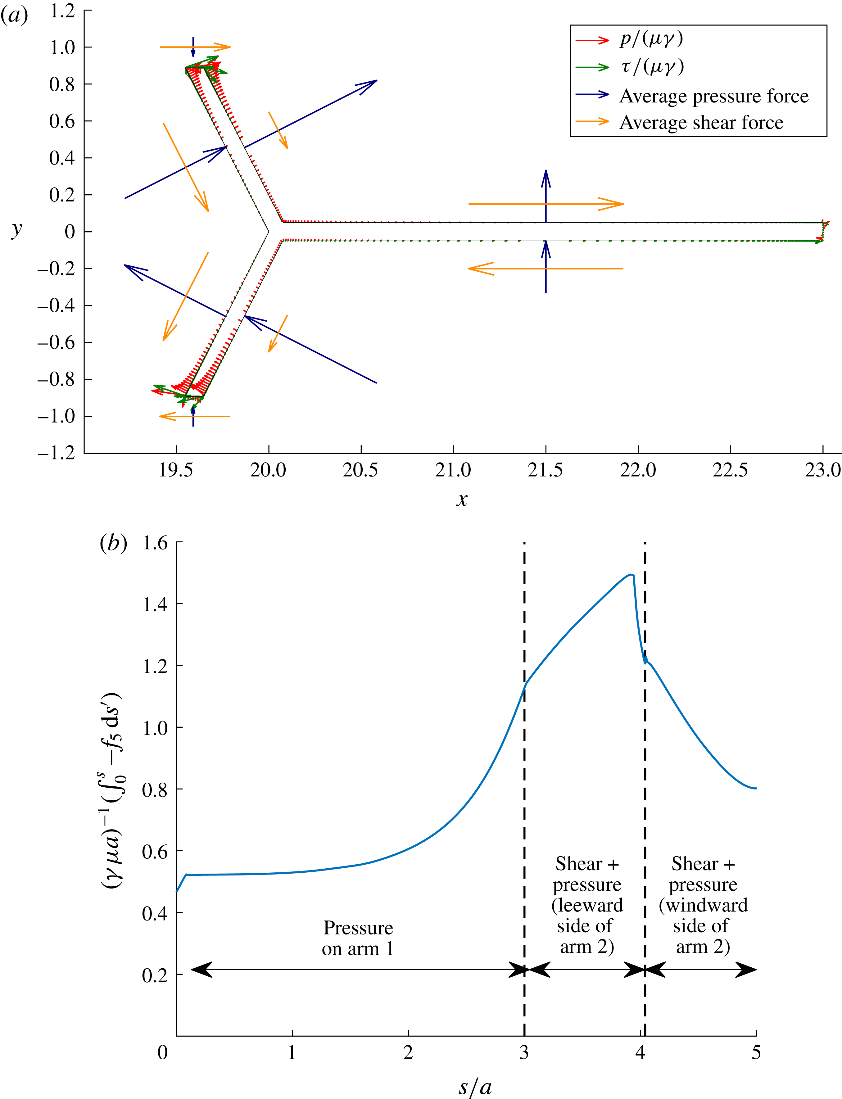
Stresses on ring cross-section contributing to particle rotation rate. (a) Plotting forces on the cross-section such that
 $\boldsymbol{f}^{\prime }\boldsymbol{\cdot }\boldsymbol{e}_{\boldsymbol{x}}=-f_{0}$
and
 $\boldsymbol{f}^{\prime }\boldsymbol{\cdot }\boldsymbol{e}_{\boldsymbol{y}}=-f_{5}$
for a particle with aspect ratio of 25.8. These forces are decomposed into the pressure (
 $p$
) and the viscous stress (
 $\unicode[STIX]{x1D70F}$
). The pressure (
 $\rightarrow$
, red) and viscous stress (
 $\rightarrow$
, green) variation along the cross-section; total pressure force (
 $\int _{s_{1}}^{s_{2}}\text{d}s^{\prime }\,p/(\unicode[STIX]{x1D707}\unicode[STIX]{x1D6FE})$
) (
 $\rightarrow$
, blue) and total viscous force (
 $\int _{s_{1}}^{s_{2}}\text{d}s^{\prime }\,\unicode[STIX]{x1D70F}/(\unicode[STIX]{x1D707}\unicode[STIX]{x1D6FE})$
) (
 $\rightarrow$
, yellow) per unit circumference on each face of each arm is plotted. (b) Cumulative value of
 $-f_{5}$
along the cross-section from tip of arm 1 (
 $s=0$
) to a point s along arm 1. Here,
 $\unicode[STIX]{x1D6FE}$
is the shear rate of the simple shear flow and
 $\unicode[STIX]{x1D707}$
is the viscosity of the fluid.

where
 $\text{d}s^{\prime }$
represents the elemental length along the tangent to the cross-sectional contour and
 $s^{\prime }$
represents the position along the contour such that
 $s^{\prime }=0$
corresponds to the point on the outer edge for which
 $y_{s}=0$
. A negative value of this torque, which is the torque opposite to the vorticity direction, implies alignment. The moment arm for forces along
 $\boldsymbol{e}_{\boldsymbol{y}}$
, i.e.
 $x$
, scales with the particle size (
 $x\sim R$
), while the moment arm for the forces acting along
 $\boldsymbol{e}_{\boldsymbol{x}}$
, i.e.
 $y$
, scales with the cross-sectional dimension (
 $y\sim a$
). Thus, at a sufficiently high aspect ratio,
 $A$
, the torque due to the force along
 $\boldsymbol{e}_{\boldsymbol{y}}$
(
 $-f_{5}$
) alone is important. Figure 3(a) shows the part of the force per unit area (
 $\boldsymbol{f}^{\prime }$
) acting on the cross-section that contributes to the torque, at
 $\unicode[STIX]{x1D719}=0$
, such that
 $\boldsymbol{f}^{\prime }\boldsymbol{\cdot }\boldsymbol{e}_{\boldsymbol{x}}=-f_{0}$
and
 $\boldsymbol{f}^{\prime }\boldsymbol{\cdot }\boldsymbol{e}_{\boldsymbol{y}}=-f_{5}\boldsymbol{\cdot }\boldsymbol{f}^{\prime }$
is decomposed into a normal force which is due to pressure (
 $p$
) and a tangential force which is due to the shear or viscous stress (
 $\unicode[STIX]{x1D70F}$
). Figure 3(a) shows the variation of pressure along with the total pressure force and total viscous force per unit circumference on each linear element of the cross-section (
 $\int \text{d}s^{\prime }\,p/(\unicode[STIX]{x1D707}\unicode[STIX]{x1D6FE})$
and
 $\int \text{d}s^{\prime }\,\unicode[STIX]{x1D70F}/(\unicode[STIX]{x1D707}\unicode[STIX]{x1D6FE})$
respectively, where
 $\unicode[STIX]{x1D6FE}$
is the shear rate of the simple shear flow and
 $\unicode[STIX]{x1D707}$
is the viscosity of the fluid). This allows for the visualization of forces that lead to a force along the positive
 $\boldsymbol{e}_{\boldsymbol{y}}$
. From figure 3(a), the pressure on average generates a force in the positive
 $\hat{\unicode[STIX]{x1D71E}}_{\infty }$
, which tries to rotate the particle towards the stable orientation. On the other hand, the viscous stress generates a force along negative
 $\hat{\unicode[STIX]{x1D71E}}_{\infty }$
which tries to tumble the particle in the vorticity direction. The viscous stress is localized near the stagnation points, which are at the tip of each arm, and thus acts on a smaller area. The pressure decays slowly along the arms due to small velocity gradients (except for a small region near the stagnation point) and so it acts on a larger area. The obtuse angle of arm 2 with the flow direction ensures the pressure generates a force in the positive
 $\hat{\unicode[STIX]{x1D71E}}_{\infty }$
direction. Pressure on arm 1 also generates a force in the positive
 $\hat{\unicode[STIX]{x1D71E}}_{\infty }$
direction. Figure 3(b) shows the variation of
 $\int _{0}^{s}\text{d}s^{\prime }(-f_{5})$
along the cross-section from the tip of arm 1 (
 $s=0$
) to the point of intersection of arms 2 and 3. The pressure on each arm makes a positive contribution to
 $(-f_{5})$
, while the viscous stress mainly near the tip of arm 2 and most of the windward side of arm 2 makes a negative contribution to (
 $-f_{5}$
). While the viscous stresses try to tumble the particle irrespective of the cross-sectional shape, the pressure force for certain cross-sections leads to alignment.
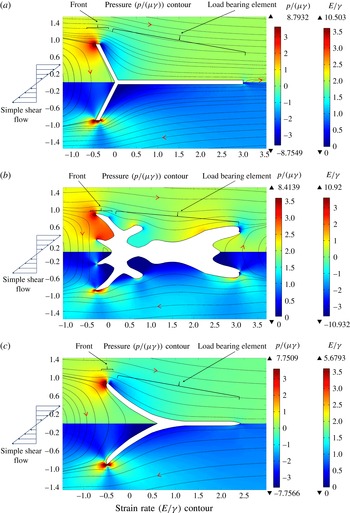
Pressure, strain rate contours and streamlines for different cross-sections: (a)
 $Y$
-shaped cross-section, (b) cross-section with a branched load-bearing element and (c) cross-section with streamlined load-bearing element. The top half shows the pressure (
 $p/(\unicode[STIX]{x1D6FE}\unicode[STIX]{x1D707})$
) contour, while the bottom half shows the strain rate (
 $E/\unicode[STIX]{x1D6FE}$
) contour.

Figure 4(a) shows the pressure, strain rate and streamlines obtained from the solution of the 2-D Stokes flow problem near a
 $Y$
-shaped cross-section. The strain rate is defined as
 $E=(0.5(\unicode[STIX]{x1D735}\boldsymbol{u}+(\unicode[STIX]{x1D735}\boldsymbol{u})^{\text{T}})\boldsymbol{ : }(\unicode[STIX]{x1D735}\boldsymbol{u}+(\unicode[STIX]{x1D735}\boldsymbol{u})^{\text{T}}))^{0.5}$
, and gives a measure of the viscous stress in the fluid. From symmetry of the particle and the simple shear flow, it can be shown that
 $\boldsymbol{f}\boldsymbol{\cdot }\hat{\boldsymbol{U}}_{\infty }(x,-y)=-\boldsymbol{f}\boldsymbol{\cdot }\hat{\boldsymbol{U}}_{\infty }(x,y)$
and
 $\boldsymbol{f}\boldsymbol{\cdot }\hat{\unicode[STIX]{x1D71E}}_{\infty }(x,-y)=\boldsymbol{f}\boldsymbol{\cdot }\hat{\unicode[STIX]{x1D71E}}_{\infty }(x,y)$
,
 $\boldsymbol{f}$
being the force per unit area acting on the particle surface. The strain rate, as shown in the bottom half of figure 4(a), is localized near the end of each arm and thus, acts on a small area generating a small force. The low pressure, relative to the pressure far away from the particle, on the right of arm 2 and top of arm 1, is created by the presence of the stagnation point on the tip of arm 2. This low pressure due to the obtuse angle made by arm 2 about the flow direction and the presence of arm 1 is utilized to generate a force on the particle along
 $\boldsymbol{e}_{\boldsymbol{y}}$
. The obtuse angle made by arm 2 ensures that the pressure force generates a positive force in the
 $y$
-direction. It can be easily envisioned that pressure generates a force in the negative
 $y$
-direction if arm 2 makes an acute angle with the flow direction. The presence of arm 1 helps to further utilize this low pressure generated on the leeward (left) side of arm 2 by providing more surface area on which the low pressure acts. It should be noted that a cross-section which is the mirror image of this
 $Y$
-shape (R-6 in figure 2
c) would not be able to align, because the sign of the forces would reverse. The pressure on top of arm 1 would generate a force in the negative
 $y$
-direction while the acute angle made by arm 2 with the flow direction would also make the pressure on it generate a force in the negative
 $y$
-direction.
The above information can be used to understand the requirements on the shape of the cross-section of aligning rings. The cross-section should be asymmetric about any plane normal to
 $\boldsymbol{e}_{\boldsymbol{x}}$
such that it has a blunt inner edge and a sharp outer edge. This generates a load-bearing element (arms 1, 2 and 3) that thins out as one approaches the outer edge utilizing the pressure to generate a counter-rotating torque. Figures 4(b,c) show the contours for pressure and strain rate (
 $E$
), along with the streamlines obtained from the solution of the 2-D Stokes problem using FEM. As illustrated by these figures, the viscous stress mainly acts in small regions around the stagnation points on the tips of the arms, generating a smaller force in comparison to the pressure force that acts on a larger projected area of the load-bearing element. The viscous force on the front will be smaller if the flow is streamlined, and thus shapes with branched load-bearing elements, as shown in figure 4(b), will tend to perform poorly. Branching not only increases the area available for the viscous stress to act, but also increases the moment arm of forces in the
 $x$
-direction, thus increasing
 $A^{\ast }$
. An unbranched load-bearing element, shown in figure 4(c), thus is ideal for alignment at low
 $A^{\ast }$
. A
 $Y$
-shaped cross-section, being the simplest shape with linear arms, was thus chosen for further analysis. A streamlined shape, as shown in figure 4(c), ensures that the viscous stress is localized near the tip of the inner edge of the cross-section and thus acts on a small area. Although optimization of the cross-section to minimize
 $A^{\ast }$
is beyond the scope of this study, our results can be the starting point for this search.
We can use these insights to rationalize the aligning or rotating nature of rings with cross-sections shown in figure 2(c). A circular cross-section does not align due to its symmetry. A pie shaped cross-section (A-1) breaks the symmetry about a plane normal to
 $\boldsymbol{e}_{\boldsymbol{x}}$
, thus allowing pressure to generate a counter-rotating torque. A
 $V$
-shaped particle (A-5) aligns at a higher
 $A^{\ast }$
as the length of the load-bearing element is smaller than for a
 $Y$
-shaped particle. Thus, we have seen that the 2-D Stokes flow problem solved using FEM can give the qualitative nature of the forces acting on rings with the given cross-section.
The solution to the mobility problem gives the dynamical parameters of the particle and thus
 $A^{\ast }$
. The dynamic parameters
 $\unicode[STIX]{x1D702}_{1}$
and
 $\unicode[STIX]{x1D702}_{2}$
are identically equal to zero for fore–aft symmetric shapes, as orientations
 $\boldsymbol{p}$
and
 $-\boldsymbol{p}$
are equivalent. The rotation parameter,
 $\unicode[STIX]{x1D706}$
, obtained from BEM simulation of this mobility problem for
 $\boldsymbol{p}$
lying in the flow–gradient plane is given by
 $$\begin{eqnarray}\unicode[STIX]{x1D706}=\frac{\unicode[STIX]{x1D6FE}^{-1}(\unicode[STIX]{x1D74E}_{\boldsymbol{p}})\boldsymbol{\cdot }\hat{\unicode[STIX]{x1D734}}_{\infty }-0.5}{(\,\boldsymbol{p}\boldsymbol{\cdot }\hat{\unicode[STIX]{x1D71E}}_{\infty })^{2}-0.5},\end{eqnarray}$$
 $\unicode[STIX]{x1D706}$
and
 $A^{\ast }$
variation for different shapes. (a) Variation of
 $A^{\ast }$
with thickness of one arm at a time for a
 $Y$
-shaped cross-section shown in figure 2(b).
 $A^{\ast }$
variation with
 $t_{1}/l_{2}$
for
 $t_{2}/l_{2}=0.1$
(▪, blue); with
 $t_{2}/l_{2}$
for
 $t_{1}/l_{2}=0.1$
(●, red); and with
 $t_{2}/l_{2}$
for
 $t_{1}/l_{2}=0.0125$
(
 $\star$
).
 $l_{1}/l_{2}=3$
and
 $\unicode[STIX]{x1D713}=0.5\unicode[STIX]{x03C0}$
for all three curves. (b)
 $\unicode[STIX]{x1D706}+1$
variation with aspect ratio of the particle (
 $A$
) for a
 $Y$
-shaped cross-section with
 $\unicode[STIX]{x1D713}=0.5\unicode[STIX]{x03C0}$
and
 $t_{1}/l_{1}=t_{2}/l_{1}=0.1$
. (c) Contour map of
 $A^{\ast }$
with
 $\unicode[STIX]{x1D713}$
and
 $l_{1}/l_{2}$
for a
 $Y$
-shaped cross-section with
 $t_{1}/l_{2}=t_{2}/l_{2}=0.0125$
. (d) Variation of
 $\unicode[STIX]{x1D706}+1$
with
 $A$
for a
 $Y$
-shaped cross-section (
 $\unicode[STIX]{x1D713}=0.65\unicode[STIX]{x03C0}$
,
 $l_{1}=2l_{2}$
,
 $t_{1}=t_{2}=0.0125l_{2}$
), mirror image of the
 $Y$
-shaped cross-section (figure 2(c) R-6) with (
 $\unicode[STIX]{x1D713}=0.65\unicode[STIX]{x03C0}$
,
 $l_{1}=2l_{2}$
,
 $t_{1}=t_{2}=0.0125l_{2}$
) and a circular cross-section (figure 2(c) R-1).

where
 $\unicode[STIX]{x1D6FE}$
is the shear rate of the simple shear flow. Figure 5(a) presents predictions for
 $Y$
-shaped particles with
 $\unicode[STIX]{x1D713}=\unicode[STIX]{x03C0}/2$
, also referred to as
 $T$
-shaped particles. Such shapes are of practical interest due to ease of fabrication using multi-step lithography (Foulds & Parameswaran Reference Foulds and Parameswaran2006). The critical aspect ratio decreases with decreasing arm thickness (
 $t_{1}/l_{2}$
and
 $t_{2}/l_{2}$
) as seen in figure 5(a) for a fixed value of
 $l_{1}/l_{2}=3$
. This is mainly due to reduction in the viscous stress acting on the particle, confirming that viscous stress increases
 $A^{\ast }$
. Thus, arms of zero thickness can be assumed to be better for all values of
 $l_{1}/l_{2}$
and
 $\unicode[STIX]{x1D713}$
. Figure 5(b), shows the variation of the rotation parameter,
 $\unicode[STIX]{x1D706}$
, with aspect ratio,
 $A$
. (
 $\unicode[STIX]{x1D706}+1$
) rapidly decreases with increasing
 $A$
, attains a minimum value that is less than zero and then slowly returns to zero. When
 $(\unicode[STIX]{x1D706}+1)\geqslant 0$
, the time period of rotation, which equals
 $4\unicode[STIX]{x03C0}/(\unicode[STIX]{x1D6FE}\sqrt{1-\unicode[STIX]{x1D706}^{2}})$
, increases as
 $\unicode[STIX]{x1D706}$
approaches
 $-1$
. This period becomes infinite at
 $\unicode[STIX]{x1D706}=-1$
and the particle aligns for the first time. Thus even though
 $A<A^{\ast }$
, due to the rapid increase in time period, the particle will remain aligned for long time durations. Once
 $\unicode[STIX]{x1D706}$
crosses
 $-1$
, the particle attains an equilibrium orientation. As shown in § 2, the angle made by
 $\boldsymbol{p}$
with gradient direction is given by
 $0.5\text{acos}(-1/\unicode[STIX]{x1D706})$
. This angle attains a maximum value when
 $\unicode[STIX]{x1D706}+1$
attains a minimum value. However, since the change in
 $\unicode[STIX]{x1D706}$
is small after attaining this minimum value the angle also changes slowly. Figure 5(c) shows the variation of
 $A^{\ast }$
with
 $\unicode[STIX]{x1D713}$
and
 $l_{1}/l_{2}$
for
 $t_{1}/l_{2}=t_{2}/l_{2}=0.0125$
, which approximates the zero-thickness limit. The contour is obtained by linear interpolation between data points using a Delaunay triangulation. The optimal value is found to be
 $A^{\ast }\approx 9$
for
 $\unicode[STIX]{x1D713}=0.65\unicode[STIX]{x03C0}$
and
 $l_{1}/l_{2}=2$
. There is a shallow valley near this optimum in which
 $A^{\ast }$
varies slowly. Thus any imperfections in particle fabrication will not change the aligning behaviour of the particle to a great extent. This also means that the particle dynamics is not strongly affected by small changes at the small length scale, as long as the general shape necessary for alignment is maintained.
Rings with
 $Y$
-shaped cross-sections have suppressed rotation at all aspect ratios in comparison to rings with circular cross-sections as evident in figure 5(d). This primarily comes due to the strong counter-rotating pressure force, absent in rings with a circular cross-section. It should be noted that rings with cross-sectional shapes studied in Singh et al. (Reference Singh, Koch and Stroock2013), as shown in figure 2(a), do not have suppressed rotation at small aspect ratios. This is primarily because the magnitude of the pressure force acting at the stagnation point is lower in comparison to a
 $Y$
-shaped cross-section with thin arms. The rings with
 $Y$
-shaped cross-sections of aspect ratio,
 $A$
, somewhat smaller than
 $A^{\ast }$
could have a similar practical utility as aligning rings because of the large increase in the time period of rotation of the ring at all aspect ratios. Apart from alignment, the particle rotation rate can be significantly increased, as shown in figure 5(d), by using a shape that is a mirror image of the
 $Y$
-shaped cross-section (R-6). This is because the pressure that was originally inducing a counter-rotating torque is now generating a torque in the vorticity direction leading to enhanced tumbling. Enhanced rotation of particles could increase the viscosity of the suspension for the same volume fraction of the particles. At high enough particle concentrations, enhanced rotation could lead to more frequent contacts between particles leading to a larger increase in stress in the suspension. High-aspect-ratio conducting particles with enhanced rotation could be embedded in composites during curing to increase the thermal conductivity of the final material.
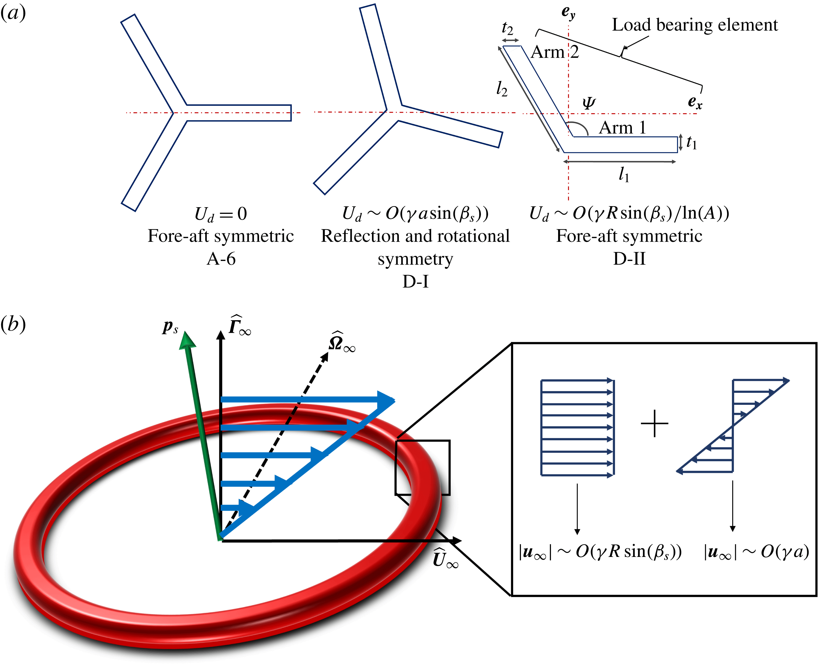
(a) Three types of cross-sectional shapes that can generate different scaling of cross-stream drift. (b) Flow field near the cross-section decomposed into a local uniform flow and a local simple shear flow that are
 $O(\unicode[STIX]{x1D6FE}R\sin (\unicode[STIX]{x1D6FD}_{s}))$
and
 $O(\unicode[STIX]{x1D6FE}a)$
respectively.

4.2 Fore–aft asymmetric particles that align and drift
Fore–aft asymmetric particles, in addition to aligning, also migrate in the cross-stream direction. Alignment of the particle can be understood by observing the local flow field around the particle when
 $\boldsymbol{p}=\hat{\unicode[STIX]{x1D71E}}_{\infty }$
, as described earlier. Here, we describe the mechanism leading to the cross-stream drift velocity of the particle (
 $U_{d}$
) once it is aligned and ways of controlling it by manipulating the cross-sectional shape. Different symmetries of cross-sectional shapes lead to different orders of magnitude of the drift velocity (
 $U_{d}=|(\boldsymbol{U}_{\boldsymbol{p}}-\boldsymbol{u}^{\infty }(\boldsymbol{r}_{\mathit{COM}}))\boldsymbol{\cdot }\hat{\unicode[STIX]{x1D71E}}_{\infty }|$
) as shown in figure 6(a). The direction of the cross-stream drift velocity depends on
 $\boldsymbol{p}$
and the cross-sectional shape of the particle. The stable orientation of the particle,
 $\boldsymbol{p}_{\boldsymbol{s}}$
, is chosen such that
 $\boldsymbol{p}_{\boldsymbol{s}}\boldsymbol{\cdot }\boldsymbol{U}_{\boldsymbol{p}}>0$
. This choice is made after obtaining the direction of
 $\boldsymbol{U}_{\boldsymbol{p}}$
from BEM calculation without loss of generality. A particle that is aligned along
 $-\boldsymbol{p}_{\boldsymbol{s}}$
would have a cross-stream migration in the opposite direction. A general cross-sectional shape will have a drift velocity that scales as
 $\unicode[STIX]{x1D6FE}R\sin (\unicode[STIX]{x1D6FD}_{s})/\ln (A)$
(figure 6
a D-II). However, a cross-section with rotational and reflectional symmetry, as shown in figure 6(a) D-I, generates
 $U_{d}$
that scales as
 $\unicode[STIX]{x1D6FE}a\sin (\unicode[STIX]{x1D6FD}_{s})$
. On the other hand, fore–aft symmetry of the cross-section leads to no cross-stream drift. The mechanism leading to cross-stream drift can be understood by obtaining the lift force on the particle when it is held stationary and oriented along its stable orientation (
 $\boldsymbol{p}=\boldsymbol{p}_{\boldsymbol{s}}$
). At this orientation, the local flow field can be decomposed into a uniform flow field and a simple shear flow as shown in figure 6(b). The local uniform flow field due to the small angle
 $\unicode[STIX]{x1D6FD}_{s}$
of the particle with respect to the gradient axis scales as
 $\unicode[STIX]{x1D6FE}R\sin (\unicode[STIX]{x1D6FD}_{s})$
over most of the ring. The scaling for the lift force due to the local uniform flow can be understood from slender body theory (Batchelor Reference Batchelor1970). Batchelor (Reference Batchelor1970) explains that the leading-order force per unit length acting on a slender filament of high aspect ratio (
 $A\gg 1$
) is independent of the shape of the slender body and scales as
 $\unicode[STIX]{x1D707}U_{0}/\ln (A)$
,
 $U_{0}$
being the measure of the undisturbed fluid velocity. Since the only direction in the problem is the flow direction, the slender filament only experiences a drag force per unit length that scales as
 $\unicode[STIX]{x1D707}\unicode[STIX]{x1D6FE}R\sin (\unicode[STIX]{x1D6FD}_{s})/\ln (A)$
for
 $\ln (A)\gg 1$
. The details of the cross-section affect the force at a higher order in ln(A) and thus the lift force per unit length, if any, scales as
 $\unicode[STIX]{x1D707}|U_{0}|/[\ln (A)]^{2}$
. Thus, the local uniform flow field generates a lift force per unit length at each azimuthal location that scales as
 $\unicode[STIX]{x1D707}\unicode[STIX]{x1D6FE}R\sin (\unicode[STIX]{x1D6FD}_{s})/[\ln (A)]^{2}$
. The local simple shear flow generates a lift force per unit length that primarily arises due to the tilt about the gradient direction (
 $\unicode[STIX]{x1D6FD}_{s}$
). This lift force per unit length scales as
 $\unicode[STIX]{x1D707}\unicode[STIX]{x1D6FE}a\sin (\unicode[STIX]{x1D6FD}_{s})/\ln (A)$
. The net lift force for a general fore–aft asymmetric particle scales as
 $\unicode[STIX]{x1D707}\unicode[STIX]{x1D6FE}R^{2}\sin (\unicode[STIX]{x1D6FD}_{s})/[\ln (A)]^{2}$
and thus the cross-stream drift velocity scales as
 $\unicode[STIX]{x1D6FE}R\sin (\unicode[STIX]{x1D6FD}_{s})/\ln (A)$
at large aspect ratios (
 $A\gg 1$
). The contribution to drift from the local uniform flow becomes identically zero if the cross-section has both reflectional and rotational symmetry. Shapes with reflectional and rotational symmetry, shown in figure 6(a) (D-II), cannot generate a lift force in a 2-D uniform flow along two different cross-sectional orientations, and thus should have zero lift for all cross-sectional orientations by linear superposition. For such cross-sections, the drift comes from the local simple shear flow alone and scales as
 $\unicode[STIX]{x1D6FE}a\sin (\unicode[STIX]{x1D6FD}_{s})$
. Thus, depending on the symmetry properties of the cross-sectional shape the cross-stream drift scales differently. However, contributions from both the mechanisms are important for particles with low aspect ratios. The angle made by the particle with the gradient direction,
 $\unicode[STIX]{x1D6FD}_{s}=0.5\text{acos}(-1/\unicode[STIX]{x1D706})\approx [0.5|\unicode[STIX]{x1D706}+1|]^{0.5}$
, also depends on the particle geometry. The maximum value of
 $\unicode[STIX]{x1D6FD}_{s}$
depends on the capability of the shape to generate the highest counter-rotating torque. To understand this variation, consider a shape shown in figure 6(a) (D-II) and a fore–aft symmetric cross-section obtained by adding a reflection of this cross-section in a manner that keeps the particle aligned, as shown in figure 6(a) (A-6). The forces acting on the particle when
 $\boldsymbol{p}=\hat{\unicode[STIX]{x1D71E}}_{\infty }$
, will be nearly the same for the asymmetric cross-section and the top half of the fore–aft symmetric cross-section. Therefore, a fore–aft symmetric shape, A-6, can generate approximately twice the counter-rotating torque of the corresponding fore–aft asymmetric shape, D-II, at half the aspect ratio. The aspect ratio for a A-6 shape halves because the cross-sectional dimension ‘
 $2a$
’ is twice that of the D-II shape. Consequently, the maximum
 $\unicode[STIX]{x1D6FD}_{s}$
is not only higher for the A-6 than the D-II shape but also occurs at a smaller aspect ratio. Fore–aft symmetry does not allow for migration, but rotating the cross-section breaks the fore–aft symmetry and allows for a finite drift. Shapes with rotational and reflectional symmetry, as shown in figure 6(a) (D-I), have some resemblance to an equivalent fore–aft symmetric shape (A-6) and some resemblance to a fore–aft asymmetric shape (D-II). The D-I shape can align at a lower aspect ratio and have a higher
 $\unicode[STIX]{x1D6FD}_{s}$
than a D-II shape and it could have a maximum value of cross-stream drift that is larger than that for a D-II shape. However, since the scaling of
 $U_{d}$
with aspect ratio is a factor of
 $1/A$
smaller than that for a D-II shape, the drift velocity of the D-II shape becomes larger as
 $A\rightarrow \infty$
. This will be shown towards the end of this section by using specific examples. Consequently, particle migration is intertwined with the orientational dynamics of the particle and this intertwining is stronger for particles that align at low aspect ratios. We now elucidate the dependence on geometry for certain cross-sectional shapes from the solution of the mobility problem.
The alignment for rings with cross-section D-II can be understood from the previous discussion. The load-bearing element as marked in figure 6(a), allows one to envision the pressure forces that lead to alignment. For a general fore–aft asymmetric cross-section, where a similar picture is non-trivial, observing the lift force through the solution of a two-dimensional Stokes flow problem, as shown in figure 4, is a good method of comparing geometries.
Aligning particles that lack fore–aft symmetry have non-zero values of the dynamic parameters,
 $\unicode[STIX]{x1D702}_{1}$
and
 $\unicode[STIX]{x1D702}_{2}$
and thus have a constant cross-stream drift (
 $U_{d}$
). This cross-stream drift velocity as well as the dynamic parameters are obtained from the solution of the mobility problem. The rotation parameter,
 $\unicode[STIX]{x1D706}$
, is obtained by (3.2) while
 $\unicode[STIX]{x1D702}_{1}$
and
 $\unicode[STIX]{x1D702}_{2}$
are given by
 $$\begin{eqnarray}\displaystyle & \displaystyle \unicode[STIX]{x1D702}_{1}=\frac{\boldsymbol{U}_{\boldsymbol{p}}\boldsymbol{\cdot }\boldsymbol{n}}{\unicode[STIX]{x1D6FE}((\,\boldsymbol{p}\boldsymbol{\cdot }\hat{\unicode[STIX]{x1D71E}}_{\infty })^{2}-0.5)} & \displaystyle\end{eqnarray}$$
 $$\begin{eqnarray}\displaystyle & \displaystyle \unicode[STIX]{x1D702}_{2}=-\unicode[STIX]{x1D702}_{1}+\frac{\boldsymbol{U}_{\boldsymbol{p}}\boldsymbol{\cdot }\boldsymbol{p}}{(\,\boldsymbol{p}\boldsymbol{p}\mathbf{:}\boldsymbol{E}^{\infty })}. & \displaystyle\end{eqnarray}$$
Equations (4.3) and (4.4) can be obtained from (2.1) and (2.3) when the imposed flow is a simple shear flow and
 $\boldsymbol{p}$
lies in the flow-gradient plane. The drift velocity in the gradient direction for rings that align in a simple shear flow, i.e.
 $\unicode[STIX]{x1D706}<-1$
, is given by
 $$\begin{eqnarray}U_{d}=\boldsymbol{U}\boldsymbol{\cdot }\hat{\unicode[STIX]{x1D71E}}_{\infty }=\left|\frac{\unicode[STIX]{x1D6FE}}{2}\left(\unicode[STIX]{x1D702}_{1}+\unicode[STIX]{x1D702}_{2}-\frac{\unicode[STIX]{x1D702}_{2}}{\unicode[STIX]{x1D706}}\right)\sqrt{\frac{\unicode[STIX]{x1D706}+1}{2\unicode[STIX]{x1D706}}}\right|.\end{eqnarray}$$
The proportionality with
 $\sin (\unicode[STIX]{x1D6FD}_{s})\approx \unicode[STIX]{x1D6FD}_{s}\approx \sqrt{-0.5(1+\unicode[STIX]{x1D706})}$
can be seen from this equation.
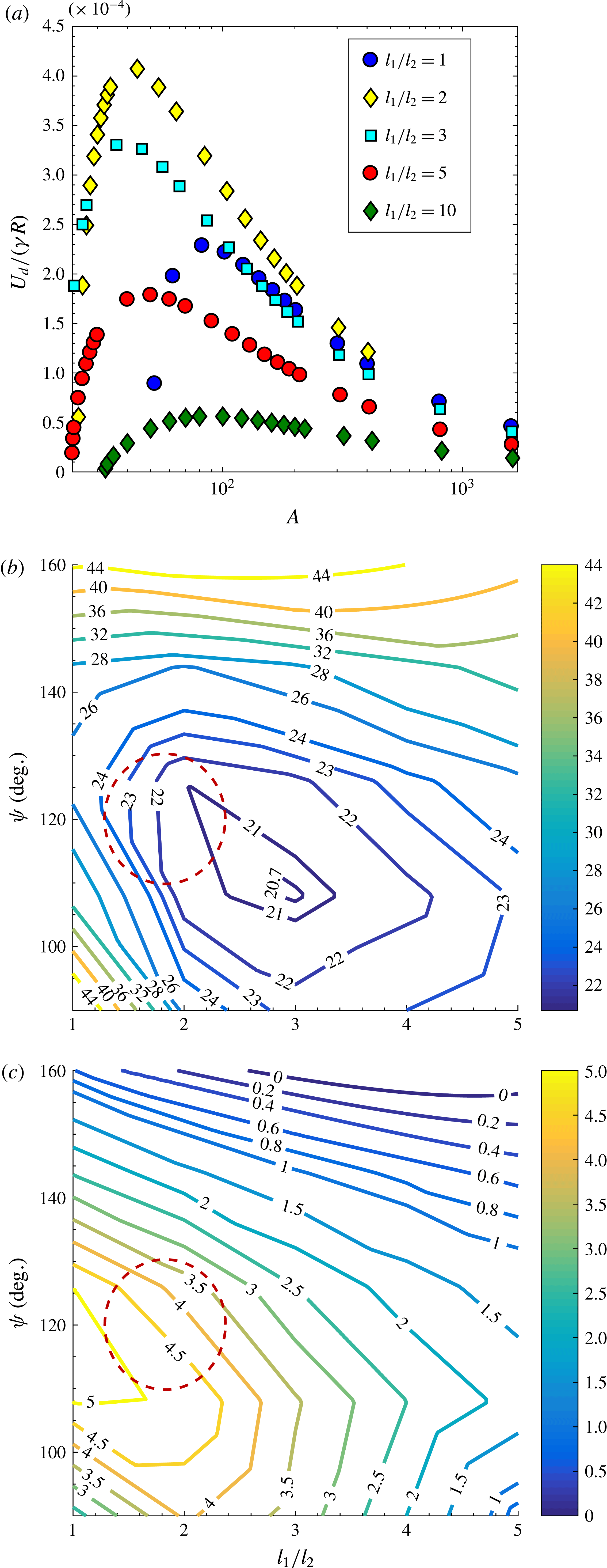
Variation of cross-stream drift velocity (
 $U_{d}$
) for shapes shown in figure 6(a) (D-II). (a) Variation of non-dimensional drift velocity,
 $\bar{U}_{d}=U_{d}/(\unicode[STIX]{x1D6FE}R)$
, with the ring aspect ratio and ratio of arm lengths (
 $l_{1}/l_{2}$
) with
 $t_{1}/l_{2}=t_{2}/l_{2}=0.0125$
and
 $\unicode[STIX]{x1D713}=0.5\unicode[STIX]{x03C0}$
. (b) Contour of
 $A^{\ast }$
with
 $\unicode[STIX]{x1D713}$
and
 $l_{1}/l_{2}$
for D-II shape with
 $t_{1}/l_{2}=t_{2}/l_{2}=0.0125$
. (c) Contour of
 $(U_{d}/(\unicode[STIX]{x1D6FE}R))\times 10^{4}$
with
 $\unicode[STIX]{x1D713}$
and
 $l_{1}/l_{2}$
for D-II shape with
 $t_{1}/l_{2}=t_{2}/l_{2}=0.0125$
.

The cross-section shown in figure 6(a) (D-II) was studied due to its resemblance with the
 $Y$
-shaped cross-section and because of ease of fabrication afforded by its flat base. Figure 7(a) shows the variation of the non-dimensional drift velocity of the particle (
 $\bar{U}_{d}=U_{d}/(\unicode[STIX]{x1D6FE}R)$
) with aspect ratio for
 $\unicode[STIX]{x1D713}=0.5\unicode[STIX]{x03C0}$
and nearly zero arm thickness (
 $t_{1}/l_{2}=t_{2}/l_{2}=0.0125$
). Reducing arm thickness reduces the area available for the viscous stresses to act as seen earlier. The variation of
 $\bar{U}_{d}$
with respect to aspect ratio shown in figure 7(a) is qualitatively similar across all shapes that can migrate across streamlines.
 $\bar{U}_{d}$
is small near the critical aspect ratio due to the vanishingly small value of
 $\unicode[STIX]{x1D6FD}_{s}$
.
 $\bar{U}_{d}$
rapidly increases to a maximum value and then decays slowly thereafter. The maximum value occurs at an aspect ratio which is close to that yielding the minimum value of
 $\unicode[STIX]{x1D706}$
or the maximum value of
 $\unicode[STIX]{x1D6FD}_{s}$
.
 $\bar{U}_{d}$
slowly decays to zero with further increase in aspect ratio. Figure 7(b) shows the contour map for the critical aspect ratio for alignment,
 $A^{\ast }$
, for varying values of
 $\unicode[STIX]{x1D713}$
and
 $l_{1}/l_{2}$
for
 $t_{1}/l_{2}=t_{2}/l_{2}=0.0125$
. The optimal value of
 $A^{\ast }$
is 20.6 and occurs approximately at
 $\unicode[STIX]{x1D713}=0.65\unicode[STIX]{x03C0}$
and
 $l_{1}/l_{2}=3$
. This minimum value of
 $A^{\ast }$
is more than double the value obtained for a
 $Y$
-shaped cross-section. This cross-section represents the top half of the
 $Y$
-shaped cross-section with nearly the same forces acting on it. Thus, the cross-sectional dimension ‘
 $2a$
’ is half that of a
 $Y$
-shaped cross-section, which leads to the near doubling of
 $A^{\ast }$
. Additional viscous stresses acting on the bottom part of arm 1 make
 $A^{\ast }$
more than double the value for an equivalent
 $Y$
-shaped cross-section. As shown in figure 7(b),
 $A^{\ast }$
varies slowly in a large region near the optimum, which suggests that the particle dynamics varies slowly for slight changes in the cross-sectional shape. Figure 7(c) shows the contour for the maximum value attained by
 $\bar{U}_{d}$
with
 $\unicode[STIX]{x1D713}$
and
 $l_{1}/l_{2}$
.
 $\bar{U}_{d}$
attains a maximum value when
 $\unicode[STIX]{x1D713}\approx 0.6\unicode[STIX]{x03C0}$
and
 $l_{1}/l_{2}\approx 1$
. However, this maximum does not coincide with parameters that give the lowest
 $A^{\ast }$
. Thus, an appropriate shape should be chosen based on the relative importance of attaining a high drift velocity and maintaining particle rigidity by restricting to a low aspect ratio. Parameters highlighted by the dotted region in figure 7(b,c) suggest a region that has a balance between alignment at low aspect ratio and attainment of a high drift velocity.
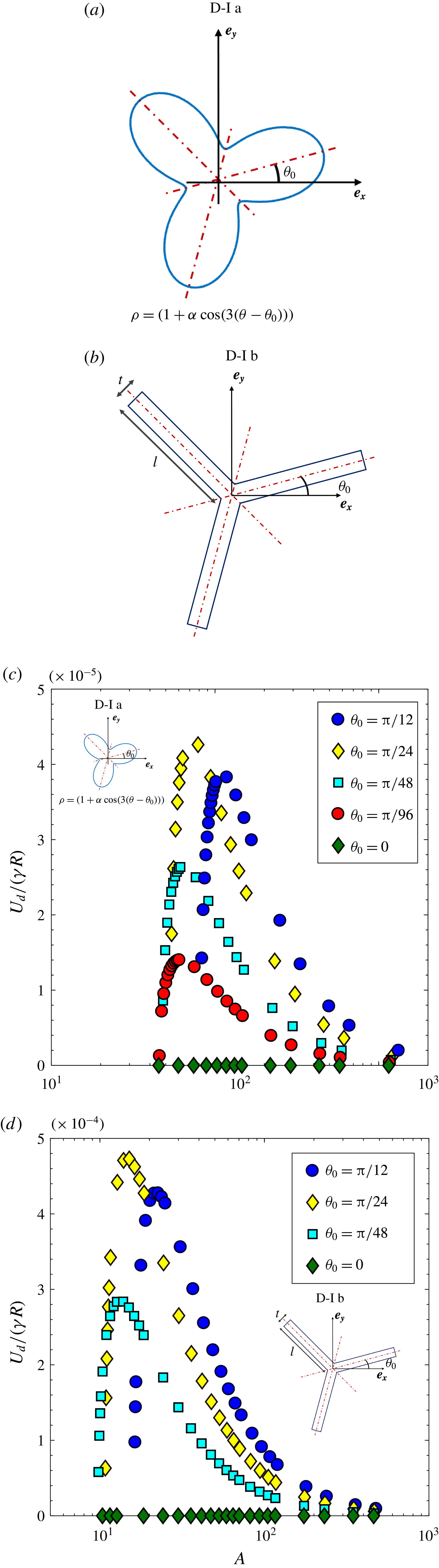
Variation of cross-stream drift velocity (
 $U_{d}$
) for shapes with reflectional and rotational symmetry (D-I shapes). (a) A cross-section given by
 $\unicode[STIX]{x1D70C}=(1+\unicode[STIX]{x1D6FC}\cos (3(\unicode[STIX]{x1D703}-\unicode[STIX]{x1D703}_{0})))$
, which is the cross-section studied in Singh et al. (Reference Singh, Koch and Stroock2013) rotated by an angle
 $\unicode[STIX]{x1D703}_{0}$
relative to
 $\boldsymbol{e}_{\boldsymbol{x}}$
. (b) D-I shape with rotational and reflectional symmetry. The angle
 $\unicode[STIX]{x1D703}_{0}$
of one of the arms with
 $\boldsymbol{e}_{\boldsymbol{x}}$
controls the degree of fore–aft asymmetry. (c) Non-dimensional drift velocity (
 $U_{d}/(\unicode[STIX]{x1D6FE}R)$
) for shape in (a) for
 $\unicode[STIX]{x1D6FC}=0.55$
. (d)
 $U_{d}/(\unicode[STIX]{x1D6FE}R)$
for shape shown in (b) with
 $l=1$
and
 $t=0.0125$
.

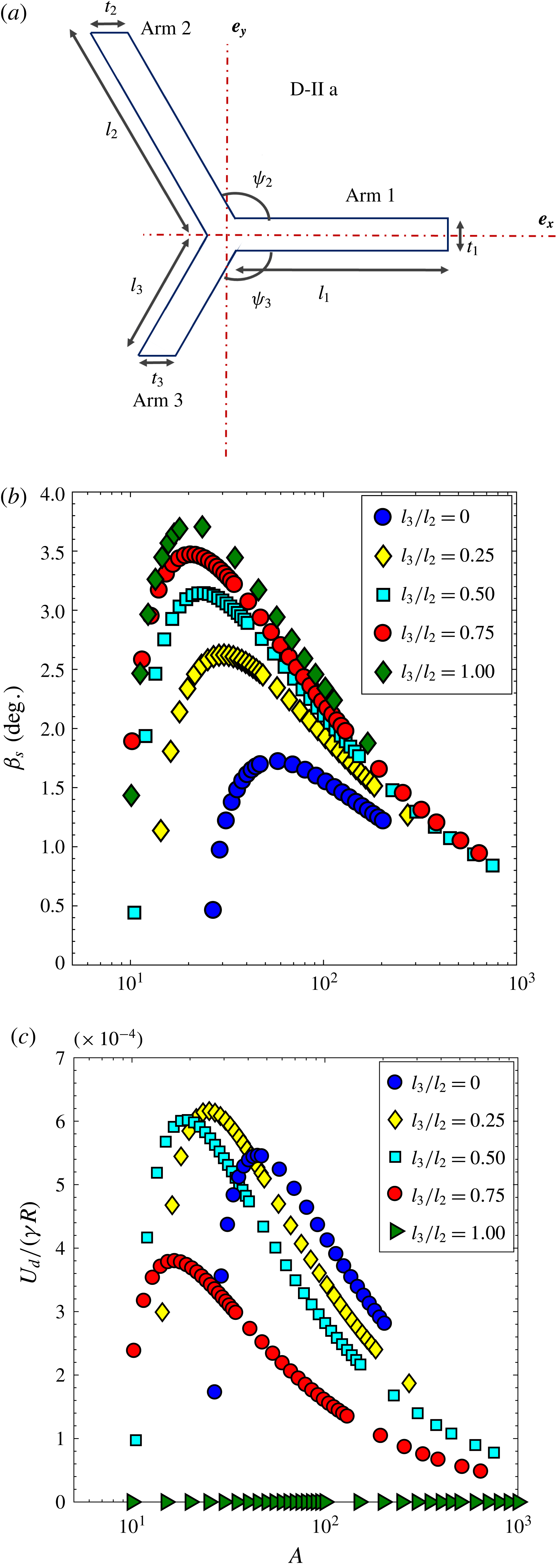
Drift velocity variation with varying degree of fore–aft asymmetry of a cross-section D-II a. (a) D-II a shape that generates varying cross-stream drift as the deviation from fore–aft symmetry is adjusted by changing length of arm 3 relative to arm 2 (i.e.
 $l_{3}/l_{2}$
). (b) Parametric variation of
 $\unicode[STIX]{x1D6FD}_{s}$
with particle aspect ratio (
 $A$
) and relative length of arm 3 (
 $l_{3}/l_{2}$
) for (D-II a) shape. (c) Parametric variation of
 $\bar{U}_{d}=U_{d}/(\unicode[STIX]{x1D6FE}R)$
with
 $A$
and (
 $l_{3}/l_{2}$
) for (D-II a) shape. In both these plots,
 $l_{1}/l_{2}=1$
,
 $\unicode[STIX]{x1D713}_{2}=\unicode[STIX]{x1D713}_{3}=0.65\unicode[STIX]{x03C0}$
and
 $t_{1}/l_{2}=t_{2}/l_{2}=t_{3}/l_{2}=0.0125$
.

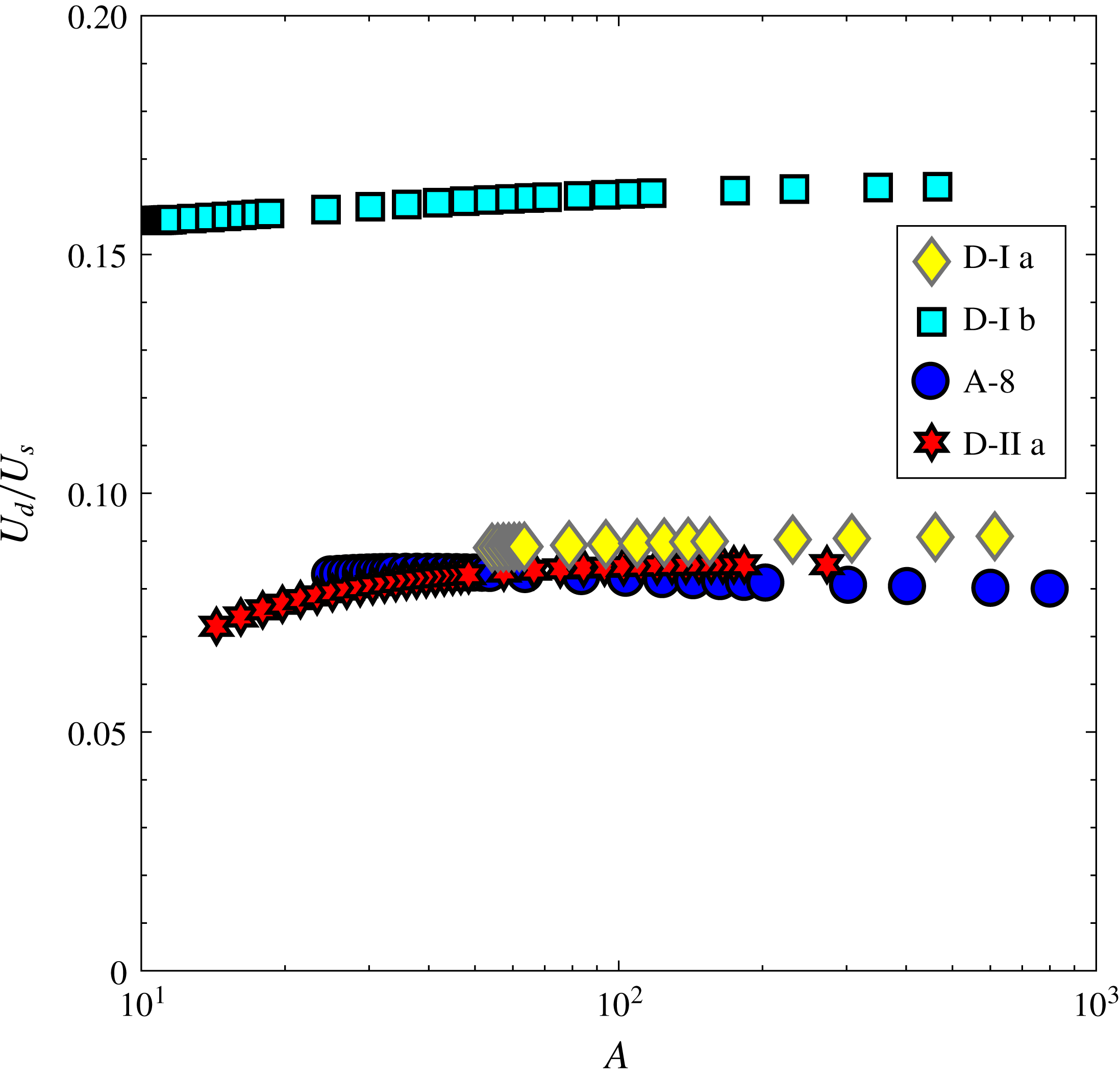
Drift velocity non-dimensionalized with the velocity obtained by scaling arguments (
 $U_{s}$
). D-I a shape (figure 8
a) with
 $\unicode[STIX]{x1D6FC}=0.55$
and
 $\unicode[STIX]{x1D703}_{0}=\unicode[STIX]{x03C0}/24$
; D-I b shape (figure 8
b) with
 $\unicode[STIX]{x1D703}_{0}=\unicode[STIX]{x03C0}/24$
and
 $t/l=0.0125$
; A-8 shape (
 $L$
-shape) with
 $l_{1}/l_{2}=2$
and
 $t_{1}/l_{2}=t_{2}/l_{2}=0.0125$
; and D-II a shape with
 $l_{1}/l_{2}=1$
,
 $l_{3}/l_{2}=0.25$
,
 $\unicode[STIX]{x1D713}_{2}=\unicode[STIX]{x1D713}_{3}=0.65\unicode[STIX]{x03C0}$
and
 $t_{1}/l_{2}=t_{2}/l_{2}=t_{3}/l_{2}=0.0125$
. The scaling for velocity for D-I a and D-I b shapes is
 $U_{s}=(\unicode[STIX]{x1D6FE}a)\sin (\unicode[STIX]{x1D6FD}_{s})$
, while the scaling for the remaining two shapes is
 $U_{s}=(\unicode[STIX]{x1D6FE}R)\sin (\unicode[STIX]{x1D6FD}_{s})/\ln (A)$
.

We considered two cross-sections with reflectional and rotational symmetry as shown in figure 8(a,b), where
 $\unicode[STIX]{x1D703}_{0}$
is the angle of rotation about
 $\boldsymbol{e}_{\boldsymbol{x}}$
. The parameters that gave the least value of
 $A^{\ast }$
for
 $\unicode[STIX]{x1D703}_{0}=0$
were chosen for each of the shapes. The parameters are
 $\unicode[STIX]{x1D6FC}=0.55$
for the shape in figure 8(a) and
 $l_{1}/l_{2}=1$
and
 $\unicode[STIX]{x1D713}=0.6\unicode[STIX]{x03C0}$
for the shape in figure 8(b). If
 $\unicode[STIX]{x1D703}_{0}=\pm \unicode[STIX]{x03C0}/6$
, these cross-section becomes symmetric about a plane normal to
 $\boldsymbol{e}_{\boldsymbol{x}}$
and thus cannot generate a force in the gradient direction when
 $\boldsymbol{p}=\hat{\unicode[STIX]{x1D71E}}_{\infty }$
because of the equivalence of the problem in flow reversal (
 $\boldsymbol{u}^{\infty }=-\boldsymbol{u}^{\infty }$
). As seen in figure 8(c),
 $\bar{U}_{d}=\text{U}_{d}/(\unicode[STIX]{x1D6FE}R)$
is an order of magnitude lower for the three-lobed cross-section in figure 8(a) in comparison to an equivalent D-II shape.
 $\bar{U}_{d}$
follows a similar trend of rapidly increasing to a maximum and slowly decaying to zero at large aspect ratios. The drift velocity for the rotated
 $Y$
-shape cross-section, i.e. D-I b shape, has values comparable with the D-II shape because rings with D-I b shaped cross-sections align at a smaller aspect ratio. Thus, rings with D-I b cross-sections generate a higher counter-rotating torque leading to a higher value of
 $\unicode[STIX]{x1D6FD}_{s}$
than the corresponding D-II shape. This increases the drift velocity of rings with D-I b shapes at lower aspect ratios. However, at higher aspect ratios rings with D-II shapes will increase
 $\bar{U}_{d}$
due to a stronger scaling of
 $\bar{U}_{d}$
with the particle aspect ratio,
 $A$
. The three-lobed cross-section, i.e. D-I a shape, in figure 8(a) aligns around the same aspect ratio as an equivalent D-II shape leading to similar values of
 $\unicode[STIX]{x1D6FD}_{s}$
. Thus, the drift velocity is a factor of
 $1/A$
smaller than an equivalent D-II shape as per the scaling argument. The aligning angle of the particle,
 $\unicode[STIX]{x1D6FD}_{s}$
, is a crucial factor, and the drift velocity can be augmented by increasing
 $\unicode[STIX]{x1D6FD}_{s}$
. Thus, as observed above, to control particle migration, it is pertinent to consider particle alignment as well.
We considered a cross-sectional shape, shown in figure 9(a), whose degree of asymmetry could be controlled systematically. This family of shapes allows another way of analysing the importance of particle symmetry in controlling the magnitude of
 $\bar{U}_{d}$
. This shape is fore–aft symmetric for
 $l_{3}/l_{2}=1$
and the degree of fore–aft asymmetry increases as
 $l_{3}/l_{2}$
changes from 1 to 0. Figure 9(b,c) show the variation of
 $\unicode[STIX]{x1D6FD}_{s}$
and
 $\bar{U}_{d}$
with particle aspect ratio (
 $A$
) for varying lengths of arm 3 (
 $l_{3}/l_{2}$
) for
 $l_{1}/l_{2}=1$
,
 $\unicode[STIX]{x1D713}_{2}=\unicode[STIX]{x1D713}_{3}=0.65\unicode[STIX]{x03C0}$
and
 $t_{1}=t_{2}=t_{3}=0.0125l_{2}$
.
 $\unicode[STIX]{x1D6FD}_{s}$
increases as
 $(l_{3}/l_{2})\rightarrow 1$
, but the particle approaches a fore–aft symmetric shape (i.e.
 $\unicode[STIX]{x1D702}_{1}\rightarrow 0$
and
 $\unicode[STIX]{x1D702}_{2}\rightarrow 0$
) which has no drift. The highest drift is obtained for a particle that has a balance between aligning at a low aspect ratio while still deviating sufficiently from fore–aft symmetry (i.e.
 $0<l_{3}/l_{2}<1$
) as seen in figure 9(b) for
 $l_{3}/l_{2}=0.25$
and
 $A=25.14$
. Such a shape could be used as a starting point to obtain the shapes that generate the highest drift (
 $U_{d}/(\unicode[STIX]{x1D6FE}R)$
). It should be noted that at high aspect ratios,
 $A>100$
,
 $\unicode[STIX]{x1D6FD}_{s}$
is nearly the same for all cross-sectional shapes at a given
 $A$
. Thus, at sufficiently high aspect ratios the drift is higher for the shape that possesses the highest degree of fore–aft asymmetry, as seen in figure 9(c).
The drift velocity obtained by scaling arguments earlier are verified by BEM results at large aspect ratios of the particle (
 $A$
). The variation of drift velocity (
 $U_{d}$
) non-dimensionalized with the appropriate scaling velocity (
 $U_{s}$
), depending on the mechanism of drift, is used to verify the scaling arguments presented earlier. Figure 10 shows the variation of
 $U_{d}/U_{s}$
for various shapes studied here.
 $U_{s}=\unicode[STIX]{x1D6FE}a\sin (\unicode[STIX]{x1D6FD}_{s})$
for shapes that possess reflectional and rotational symmetry (D-I shape), and
 $U_{s}=\unicode[STIX]{x1D6FE}R\sin (\unicode[STIX]{x1D6FD}_{s})/\ln (A)$
for fore–aft asymmetric cross-sections that lack reflectional and/or rotational symmetry (D-II shape). Figure 10 shows that at moderately high aspect ratios,
 $U_{d}/U_{s}$
attains a constant value, thus verifying the scaling and the mechanism for cross-stream migration mentioned earlier.
5 Conclusion
In conclusion, our calculations show that the rotational and translational dynamics of rings can be controlled by appropriately manipulating the cross-sectional shape. We elucidated the mechanism that leads to permanent alignment of particles in a simple shear flow: it is the pressure acting on the particle surface that leads to alignment. Rings with cross-sections that possess a blunt inner edge and a sharp outer edge, as shown in figure 4, acquire an equilibrium orientation in a simple shear flow. Rings with a streamlined cross-sectional shape, such as a
 $Y$
-shaped cross-section shown in figure 2(b), align at lower aspect ratios than blunter shapes due to localization of the viscous stress at any extending elements of the cross-section. The optimal shape in the family of
 $Y$
-shaped particles was shown to be
 $\unicode[STIX]{x1D713}=0.65\unicode[STIX]{x03C0}$
,
 $t_{2}/l_{2}\rightarrow 0$
,
 $t_{1}/l_{2}\rightarrow 0$
and
 $l_{1}/l_{2}=2$
. This might not be the globally optimal shape, but provides a starting point to search for shapes that align at lower aspect ratios. Rings with certain geometries, such as
 $Y$
-shaped cross-sections shown in figure 2(b), have suppressed rotation in comparison to rings with circular cross-sections (torus) at similar aspect ratios. This is an important finding as these rings remain aligned for longer periods of time than an equivalent torus and thus from a practical standpoint could mimic aligning particle dynamics.
For fore–aft asymmetric cross-sections, we elucidated the mechanism leading to cross-stream drift which could be controlled by altering the symmetry of the cross-section. Particles with fore–aft symmetric cross-sections have no drift. Particles with cross-sections that possess rotational and reflectional symmetry have drift that scales as
 $\unicode[STIX]{x1D6FE}a\sin (\unicode[STIX]{x1D6FD}_{s})$
while those that lack this symmetry have a drift that scales as
 $\unicode[STIX]{x1D6FE}R\sin (\unicode[STIX]{x1D6FD}_{s})/\ln (A)$
. We explained the important role that the aligning angle (
 $\unicode[STIX]{x1D6FD}_{s}$
) plays in determining the magnitude of the drift. In particular, certain shapes can possess a higher drift due to a higher aligning angle. Both alignment and migration of rings depends on the lift force generated by pressure and thus engineering the geometry to effectively utilize pressure and localizing the viscous stresses should be a starting point to tune motion of particles in shear flows.
A
 $T$
-shaped (A-7) and an
 $L$
-shaped (A-8) cross-section, studied in this work, are of practical interest due to ease of fabrication. These particles could be fabricated using multi-step photolithography (Foulds & Parameswaran Reference Foulds and Parameswaran2006). Techniques such as direct-ink writing (Raney & Lewis Reference Raney and Lewis2015) or optofluidic fabrication (Paulsen, Di Carlo & Chung Reference Paulsen, Di Carlo and Chung2015) could be used to fabricate more complicated geometries studied in this work. Fabrication of these particles, would not only allow for the verification of our results, but also pave the way for practical utility of these particles. The macroscopic properties of a particle suspension differ depending on tumbling or aligning behaviour of individual particles. Usually anisotropic tumbling particles cannot fully impart their anisotropy to the suspension due to orientational dispersion. On the other hand, aligning rings would lead to a high degree of anisotropy due to particle alignment near the flow–vorticity plane. Materials processed with aligning particle suspension should have a high degree of anisotropy in properties such as elastic modulus; specific stiffness; and thermal, electric and magnetic conductivity. Migrating particles could be used to impart surface properties such as scratch resistance by systematically depositing particles near the surface (Isla et al.
Reference Isla, Brostow, Bujard, Esteves, Rodriguez, Vargas and Castano2003). The viscosity of these suspensions should also be lower due to alignment along the lamellae improving the ease of processing. These materials could be manufactured on a large scale using existing material processing technologies such as injection moulding, spin casting and extrusion. Consequently, these aligning particles provide a unique opportunity to design particle suspensions with tuneable structure using existing manufacturing techniques.
Acknowledgement
This research was supported by the National Science Foundation Grant CBET-1435013.
Supplementary material
Supplementary material is available at https://doi.org/10.1017/jfm.2018.20.