1 Introduction
Turbulent convection over a rough surface is a common scenario that one often encounters in nature and in many industrial processes. For example, it can be found in the urban atmospheric boundary layer (BL), where the urban surfaces are in general not smooth, and in the deep oceans, where the sea beds and the ocean floors always have rough topographies. It is of great interest and especially useful to reveal the properties of this type of flow. In the field of fundamental research, Rayleigh–Bénard (RB) convection, i.e. a working fluid layer in a closed system heated from below and cooled from above, has long been proposed as a classical and yet simple paradigm to study the convection phenomenon (Ahlers, Grossmann & Lohse Reference Ahlers, Grossmann and Lohse2009; Lohse & Xia Reference Lohse and Xia2010; Chillà & Schumacher Reference Chillà and Schumacher2012; Sun & Zhou Reference Sun and Zhou2014). Rayleigh–Bénard convection has also been adopted as an ideal model system to search for ways to enhance the heat transport of natural convection (Jin & Xia Reference Jin and Xia2008; Zhong, Funfschilling & Ahlers Reference Zhong, Funfschilling and Ahlers2009a
; Zhong et al.
Reference Zhong, Stevens, Clercx, Verzicco, Lohse and Ahlers2009b
; Biferale et al.
Reference Biferale, Perlekar, Sbragaglia and Toschi2012; Huang et al.
Reference Huang, Kaczorowski, Ni and Xia2013; Lakkaraju et al.
Reference Lakkaraju, Stevens, Oresta, Verzicco, Lohse and Prosperetti2013). Here, the convective heat transport is usually expressed in terms of the Nusselt number
 $Nu$
, which is determined largely by the control parameters of the convection system, namely the Rayleigh number
 $Ra$
and the Prandtl number
 $Pr$
, defined as
 $$\begin{eqnarray}Ra=\frac{\unicode[STIX]{x1D6FC}g\unicode[STIX]{x1D6E5}H^{3}}{\unicode[STIX]{x1D708}\unicode[STIX]{x1D705}}\quad \text{and}\quad Pr=\frac{\unicode[STIX]{x1D708}}{\unicode[STIX]{x1D705}},\end{eqnarray}$$
where
 $\unicode[STIX]{x1D6E5}$
is the temperature difference across the fluid layer of height
 $H$
,
 $g$
is the acceleration due to gravitation, and
 $\unicode[STIX]{x1D6FC}$
,
 $\unicode[STIX]{x1D708}$
and
 $\unicode[STIX]{x1D705}$
are respectively the thermal expansion coefficient, the kinematic viscosity and the thermal diffusivity of the convecting fluid. Effective increase of convective heat transfer is of vital importance in many engineering applications, and the introduction of wall roughness has been expected to be an effective means for this. To study the fundamentals of heat transfer over rough surfaces, many experimental (Shen, Tong & Xia Reference Shen, Tong and Xia1996; Du & Tong Reference Du and Tong1998; Ciliberto & Laroche Reference Ciliberto and Laroche1999; Du & Tong Reference Du and Tong2000; Roche et al.
Reference Roche, Castaing, Chabaud and Hebral2001; Qiu, Xia & Tong Reference Qiu, Xia and Tong2005; Zhou & Xia Reference Zhou and Xia2010; Tisserand et al.
Reference Tisserand, Creyssels, Gasteuil, Pabiou, Gibert, Castaing and Chillà2011; Salort et al.
Reference Salort, Liot, Rusaouen, Seychelles, Tisserand, Creyssels, Castaing and Chillà2014; Wei et al.
Reference Wei, Chan, Ni, Zhao and Xia2014; Jiang et al.
Reference Jiang, Zhu, Mathai, Verzicco, Lohse and Sun2017; Xie & Xia Reference Xie and Xia2017), numerical (Stringano, Pascazio & Verzicco Reference Stringano, Pascazio and Verzicco2006; Shishkina & Wagner Reference Shishkina and Wagner2011; Wagner & Shishkina Reference Wagner and Shishkina2015; Jiang et al.
Reference Jiang, Zhu, Mathai, Verzicco, Lohse and Sun2017; Toppaladoddi, Succi & Wettlaufer Reference Toppaladoddi, Succi and Wettlaufer2017; Zhu et al.
Reference Zhu, Stevens, Verzicco and Lohse2017) and theoretical (Villermaux Reference Villermaux1998; Shishkina & Wagner Reference Shishkina and Wagner2011; Goluskin & Doering Reference Goluskin and Doering2016) studies on turbulent RB convection over rough plates have been carried out. Up to now, it has been widely accepted that the introduction of roughness on conducing plates could efficiently enhance the heat transport through the RB system. However, Shishkina & Wagner (Reference Shishkina and Wagner2011) recently proposed that the heat transport can also be reduced due to the decrease of the effective
 $Ra$
when the distances between the roughness elements are very small (see also figure 16 of Stringano et al.
Reference Stringano, Pascazio and Verzicco2006). The reduction of the
 $Nu$
in the presence of rough conducting plates is counterintuitive and yet interesting. We note that there is still a lack of systematic studies on this issue, and the objective of the present paper is to fill this gap.
The remainder of this paper is organized as follows. We first briefly describe the numerical methods adopted in § 2. Section 3 presents and analyses the results for heat transport obtained in rough cells and reveals the mechanism for the observed reduction of the
 $Nu$
. Finally, the work is concluded in § 4.
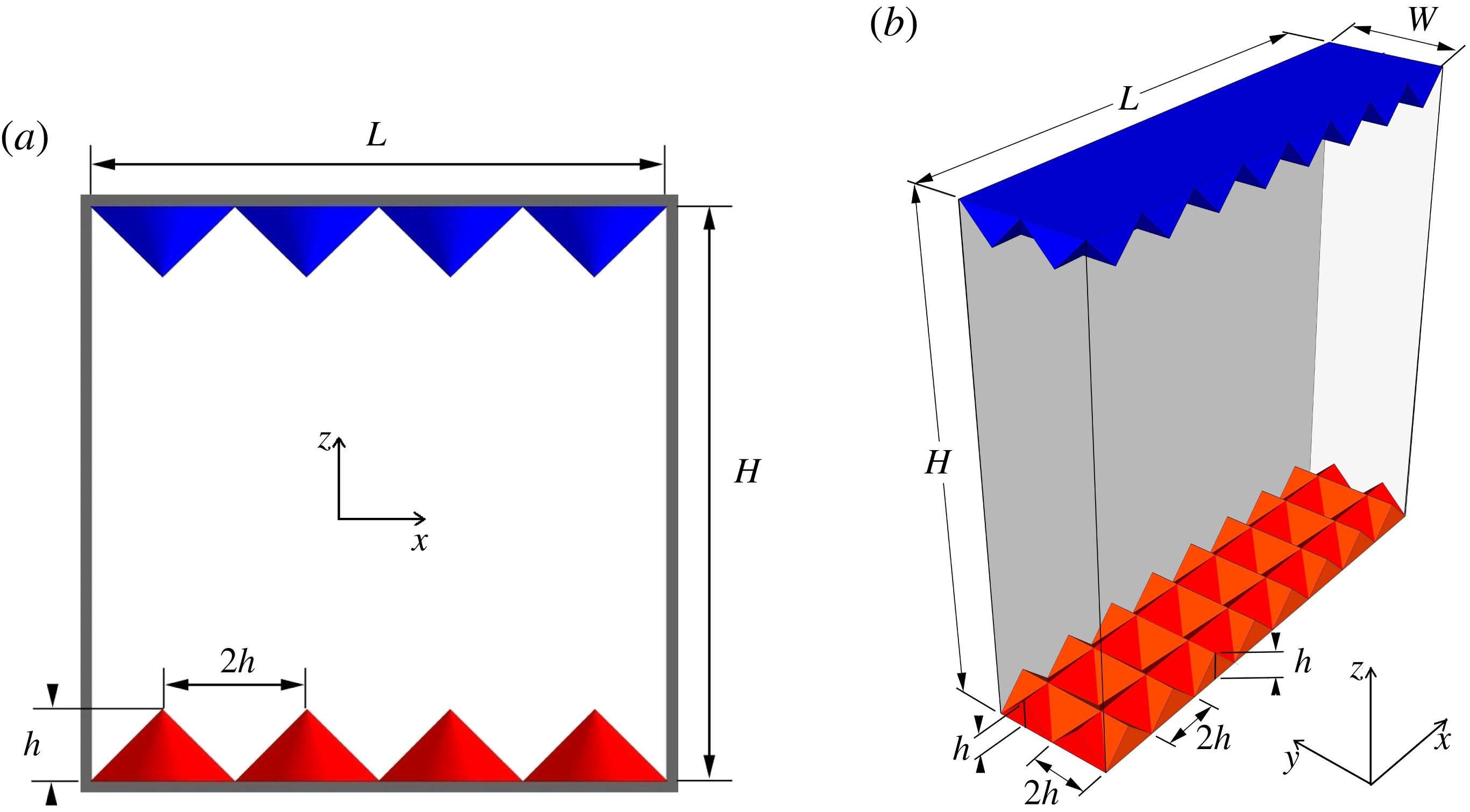
Sketches of the (a) 2D and (b) 3D convection cells with the coordinate systems. Roughness elements of height
 $h$
and base width
 $2h$
are located on each of the plates.

2 Numerical methods
We carry out direct numerical simulations (DNS) of turbulent RB convection over triangularly rough conducting plates in a two-dimensional (2D) box of height
 $H=1$
and horizontal length
 $L=1$
, as shown in figure 1(a). The triangular roughness elements have a vertex angle of 90
 $^{\circ }$
and their height and base width are
 $h$
and
 $2h$
respectively. In addition, three-dimensional (3D) DNS are performed in a rectangular cell of height
 $H=1$
, length
 $L=1$
and width
 $W=1/4$
(see figure 1
b). V-shaped grooves with a vertex angle of
 $90^{\circ }$
and with height
 $h$
and base width
 $2h$
are woven on each plate, along both the
 $L$
and the
 $W$
directions. The influence of surface roughness on heat transport is systematically studied by varying the roughness height
 $h$
. For the preset configurations, the contact area of the rough upper and lower surfaces is increased by a factor of
 $\sqrt{2}$
. When varying
 $h$
, the contact area is fixed and thus will not contribute to the variation in the
 $Nu$
for both 2D and 3D situations.
The dimensionless incompressible Oberbeck–Boussinesq equations, i.e.
 $$\begin{eqnarray}\displaystyle & \displaystyle \frac{\unicode[STIX]{x2202}\boldsymbol{u}}{\unicode[STIX]{x2202}t}+(\boldsymbol{u}\boldsymbol{\cdot }\unicode[STIX]{x1D735})\boldsymbol{u}=-\unicode[STIX]{x1D735}p+\sqrt{\frac{Pr}{Ra}}\unicode[STIX]{x1D6FB}^{2}\boldsymbol{u}+\unicode[STIX]{x1D703}\boldsymbol{z}, & \displaystyle\end{eqnarray}$$
 $$\begin{eqnarray}\displaystyle & \displaystyle \unicode[STIX]{x1D735}\boldsymbol{\cdot }\boldsymbol{u}=0, & \displaystyle\end{eqnarray}$$
 $$\begin{eqnarray}\displaystyle & \displaystyle \frac{\unicode[STIX]{x2202}\unicode[STIX]{x1D703}}{\unicode[STIX]{x2202}t}+(\boldsymbol{u}\boldsymbol{\cdot }\unicode[STIX]{x1D735})\unicode[STIX]{x1D703}=\sqrt{\frac{1}{RaPr}}\unicode[STIX]{x1D6FB}^{2}\unicode[STIX]{x1D703}, & \displaystyle\end{eqnarray}$$
were solved using a fourth-order finite-difference scheme with staggered grids. Here,
 $\boldsymbol{u}$
,
 $\unicode[STIX]{x1D703}$
and
 $p$
are respectively the velocity, temperature and kinematic pressure fields and
 $\boldsymbol{z}$
is the unit vector along the vertical direction. Our numerical code has been extensively validated and adopted in previous studies (Bao et al.
Reference Bao, Chen, Liu, She, Zhang and Zhou2015; Chen et al.
Reference Chen, Bao, Yin and She2017). No-penetration and no-slip boundary conditions were applied to all solid boundaries for the velocity fields. For temperature, the vertical sidewalls were chosen to be adiabatic (no flux), while the temperature was fixed at
 $\unicode[STIX]{x1D703}_{cold}=-0.5$
and
 $\unicode[STIX]{x1D703}_{hot}=0.5$
for the upper and lower rough plates respectively, and thus the temperature difference across the fluid layer was
 $\unicode[STIX]{x1D6E5}=\unicode[STIX]{x1D703}_{hot}-\unicode[STIX]{x1D703}_{cold}=1$
. An immersed boundary method was applied to track the boundaries of the roughness elements (Fadlun et al.
Reference Fadlun, Verzicco, Orlandi and Mohd-Yusof2000). We simulated over the range
 $10^{7}\leqslant Ra\leqslant 10^{11}$
for 2D cases, while
 $Ra$
was fixed at
 $10^{8}$
for 3D cases. In both the 2D and the 3D simulations,
 $Pr=0.7$
, corresponding to a working fluid of air (du Puits et al.
Reference du Puits, Li, Resagk and Thess2014). Non-equidistant meshes were implemented and the computational meshes were refined close to all solid surfaces. The grid resolution was chosen to reveal all scales of turbulent convection (Shishkina et al.
Reference Shishkina, Stevens, Grossmann and Lohse2010) and the thermal BLs were resolved with at least 16 grid points for all runs. Specifically,
 $2560\times 3456$
grid points were used for
 $Ra=10^{11}$
(2D) and
 $512\times 128\times 624$
for
 $Ra=10^{8}$
(3D).
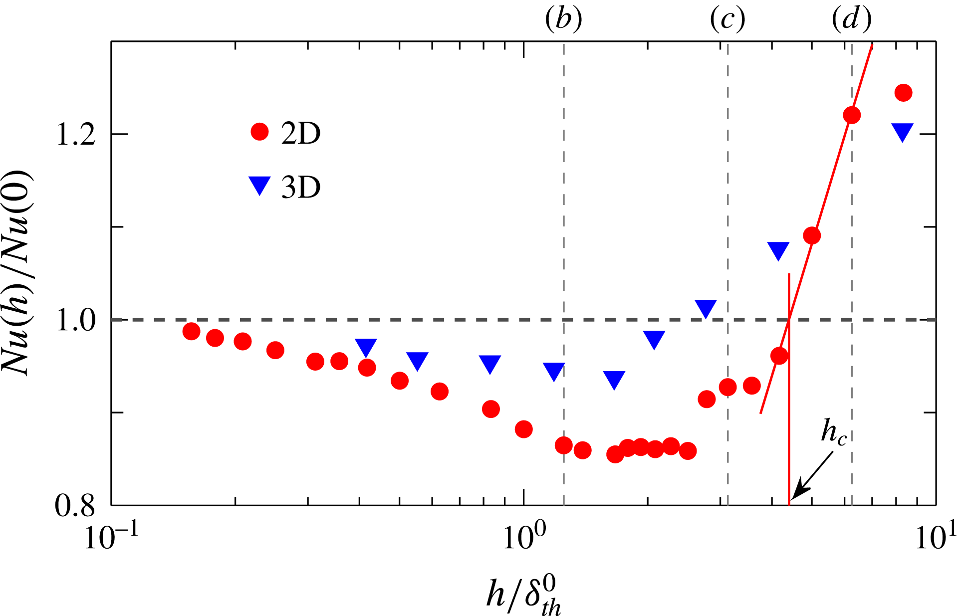
The ratio
 $Nu(h)/Nu(0)$
as a function of the normalized roughness height
 $h/\unicode[STIX]{x1D6FF}_{th}^{0}$
obtained at
 $Ra=10^{8}$
for 2D (triangles) and 3D (circles) simulations. Here,
 $\unicode[STIX]{x1D6FF}_{th}^{0}$
is the thermal BL thickness obtained in the smooth cell using
 $\unicode[STIX]{x1D6FF}_{th}^{0}=1/[2Nu(0)]$
. The red solid lines show the determination of
 $h_{c}$
, which is the roughness height at which
 $Nu(h_{c})/Nu(0)=1$
. The three vertical dashed lines mark the roughness heights that correspond respectively to figure 3(b–d).

3 Results and discussion
We first study the effects of roughness on the measured Nusselt number
 $Nu$
, which is calculated as
 $Nu=\sqrt{RaPr}\langle w\unicode[STIX]{x1D703}\rangle -\langle \unicode[STIX]{x2202}\unicode[STIX]{x1D703}/\unicode[STIX]{x2202}z\rangle$
, where
 $w$
is the vertical component of the velocity field and
 $\langle \cdot \rangle$
indicates the average over time and over the mid-height horizontal plane. We checked that the variation in
 $Nu$
calculated at different vertical positions in the core part of the convection cell between the roughness elements was smaller than
 $1\,\%$
for all of the simulations. All statistics were collected over more than 500 free-fall time units after the convective flow in the cell had been fully developed. Figure 2 shows the measured
 $Nu$
as a function of the normalized roughness height
 $h/\unicode[STIX]{x1D6FF}_{th}^{0}$
, obtained at
 $Ra=10^{8}$
for both the 2D and the 3D results. Here,
 $Nu(h)$
is normalized by
 $Nu(h=0)$
of the smooth cell to show the enhancement/reduction effects, and
 $\unicode[STIX]{x1D6FF}_{th}^{0}$
is the thermal BL thickness for the smooth wall case estimated from
 $\unicode[STIX]{x1D6FF}_{th}^{0}=1/[2Nu(0)]$
. Despite the different magnitudes, both data sets exhibit some kind of similar trend, i.e.
 $Nu(h)$
first decreases at small roughness heights, reaches a minimum and then increases. Two different regimes can be identified: the
 $Nu$
reduction regime where the overall heat transport is depressed and the
 $Nu$
enhancement regime where an increase of heat flux is achieved. The division between the two regimes gives a critical roughness height
 $h_{c}$
at which
 $Nu(h)$
crosses the value of
 $Nu(h=0)$
, as shown by the red solid lines in figure 2. The observed reduction in
 $Nu(h)$
is quite counterintuitive: now the increased contact area provided by the rough surfaces does not promote the heat flux but rather impedes it. It should be noted that Du & Tong (Reference Du and Tong1998) found that the effect of rough walls on
 $Nu$
is negligible if the height of the roughness elements is smaller than the thermal BL thickness for the smooth wall case. One would thus expect
 $Nu(h)/Nu(0)\approx 1$
for
 $h/\unicode[STIX]{x1D6FF}_{th}^{0}\lesssim 1$
. In the present study, however,
 $Nu(h)/Nu(0)<1$
is clearly observed over the range
 $h/\unicode[STIX]{x1D6FF}_{th}^{0}<2.5$
(
 $h/\unicode[STIX]{x1D6FF}_{th}^{0}<4.4$
) with a maximal reduction of
 $6.3\,\%$
(
 $15\,\%$
) for the 3D (2D) simulations (at
 $Ra=10^{8}$
; see figure 2). It is really surprising that
 $Nu$
is suppressed in such a wide parameter regime.
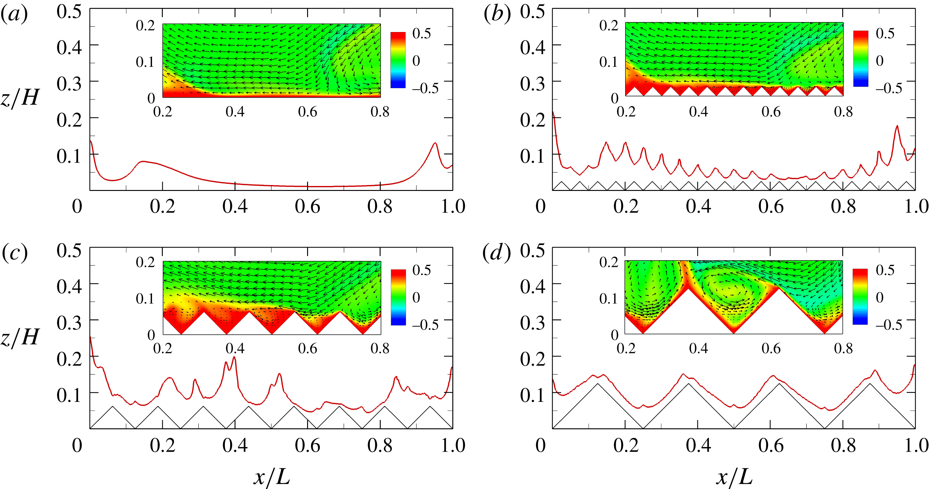
The thermal BL thicknesses,
 $\unicode[STIX]{x1D6FF}_{th}(x)$
(red curves), in the
 $z$
-direction near the bottom plate as a function of the horizontal position
 $x/L$
, determined from the time-averaged temperature profiles using the ‘slope’ method (Zhou & Xia Reference Zhou and Xia2013) and obtained at
 $Ra=10^{8}$
for 2D simulations. The insets show the corresponding instantaneous snapshots of the temperature (colour) and velocity (arrows) fields near the centre of the bottom plate. The data are obtained in the smooth cell (a) and in the rough cells with triangular roughness elements (black lines) of height
 $h/h_{c}=$
(b) 0.28, (c) 0.71 and (d) 1.42. The corresponding movie is available in the supplementary material (https://doi.org/10.1017/jfm.2017.786).

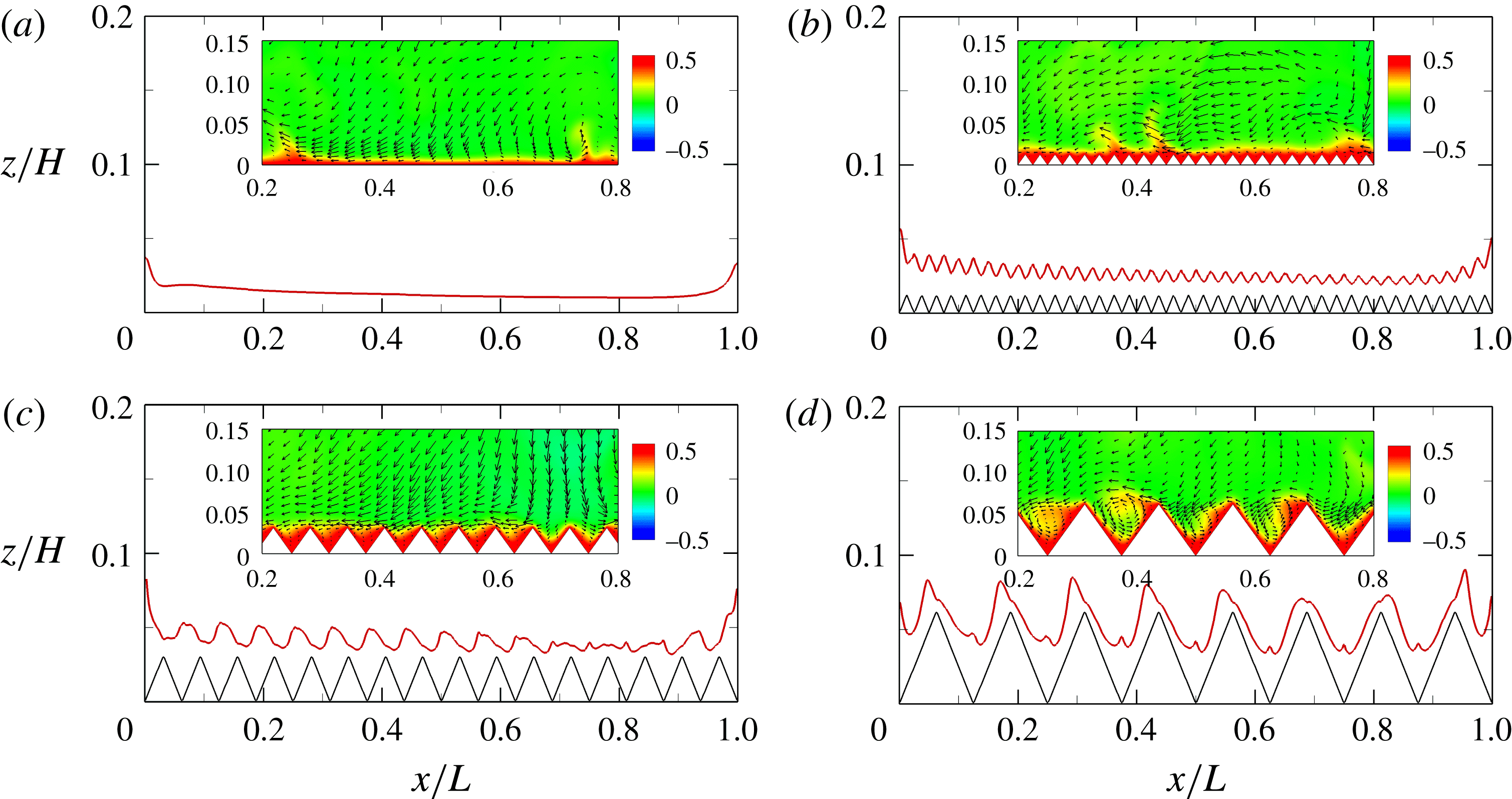
The thermal BL thicknesses,
 $\unicode[STIX]{x1D6FF}_{th}(x)$
(red curves), as a function of
 $x/L$
, taken at
 $y=W/2$
near the bottom plate and at
 $Ra=10^{8}$
for 3D simulations. The insets show the corresponding instantaneous snapshots of the temperature (colour) and velocity (arrows) fields within the vertical plane at
 $y=W/2$
. The data are obtained in the smooth cell (a) and in the rough cells with roughness heights
 $h/h_{c}=$
(b) 0.34, (c) 0.84 and (d) 1.68.

What is the physical reason for heat-transfer reduction by roughness surfaces? We note that for the present parameter ranges the convective flow is still in the so-called ‘classical’ regime (Zhu et al.
Reference Zhu, Stevens, Verzicco and Lohse2017) where the global convective heat transport is restricted mainly by thermal BLs (Ahlers et al.
Reference Ahlers, Grossmann and Lohse2009). This prompts us to directly investigate the spatial distribution of thermal BL thicknesses,
 $\unicode[STIX]{x1D6FF}_{th}(x)$
, in the cells with and without roughness. Figures 3(a) and 4(a) show, for the 2D and 3D simulations respectively,
 $\unicode[STIX]{x1D6FF}_{th}(x)$
along the bottom plate obtained at
 $Ra=10^{8}$
in the smooth cells. Here,
 $\unicode[STIX]{x1D6FF}_{th}$
is determined using the ‘slope’ method (Zhou & Xia Reference Zhou and Xia2013), i.e. the position at which the tangent of the time-averaged temperature profile at the plate crosses the bulk temperature. Due to the rising plumes near the sidewalls and the strong shear induced by the large-scale circulation (LSC), the thermal BL is thicker at the two ends but much thinner in the central regions.
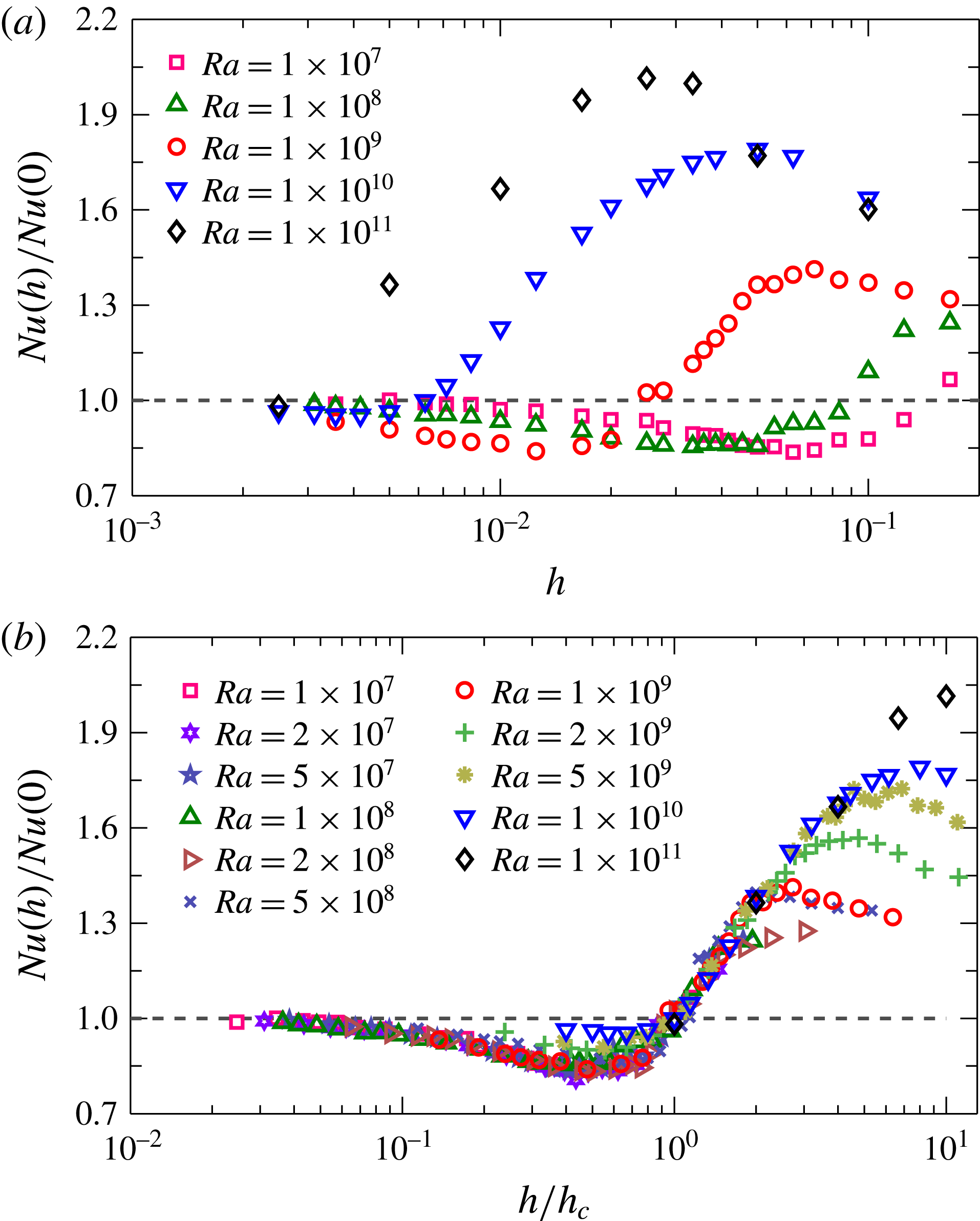
The ratio of
 $Nu(h)/Nu(0)$
as a function of (a)
 $h$
and (b)
 $h/h_{c}$
for
 $Ra$
varying from
 $10^{7}$
to
 $10^{11}$
for 2D simulations.

Figures 3(b) and 4(b) display the horizontal distributions of
 $\unicode[STIX]{x1D6FF}_{th}$
obtained in rough cells with
 $h/h_{c}=0.28$
(2D) and
 $h/h_{c}=0.34$
(3D), which are both within the
 $Nu$
reduction regime. Compared with the respective smooth cases, variations with
 $x/L$
of scale
 $h$
are imposed on
 $\unicode[STIX]{x1D6FF}_{th}$
over the rough surfaces, i.e.
 $\unicode[STIX]{x1D6FF}_{th}$
reaches a local minimum at the tips of the roughness elements, while a local maximum of
 $\unicode[STIX]{x1D6FF}_{th}$
occurs above the valleys of the cavity regions between the adjacent rough elements. To reveal how these patterns are developed, we look closely into the flow structures near the bottom plate, as illustrated in the insets of figures 3(b) and 4(b). It is seen that the hot fluid is trapped inside the cavity regions. Due to the relatively low
 $Ra$
or small
 $h$
, the flow in the cavities is dominated by the viscosity of the fluid and the trapped hot fluid cannot be well mixed, i.e. the flow in the bulk cannot penetrate into the cavities. The accumulation of the hot fluid thus thickens the thermal BLs in the cavity regions and correspondingly impedes the global heat transport through the system. The same processes can be observed for the cold fluid near the top plate. This explains why the heat transport is reduced by the roughness. It should be noted that the present mechanism of heat-flux reduction is quite similar to that of drag reduction by riblets in turbulent channel flow (Choi, Moin & Kim Reference Choi, Moin and Kim1993) and in turbulent Taylor–Couette flow (Zhu et al.
Reference Zhu, Ostilla-Mónico, Verzicco and Lohse2016). Figures 3(c) and 4(c) show the results for
 $\unicode[STIX]{x1D6FF}_{th}$
at
 $h/h_{c}=0.71$
(2D) and 0.84 (3D). As
 $h$
is increased, the flow inside the cavities becomes stronger and some secondary vortices start to be generated by the LSC. However, at these values of
 $h$
, the secondary vortices are too still weak to efficiently mix the fluid in all cavities and in the bulk. Therefore, the global heat transport is still less than that in the smooth wall case.
Figures 3(d) and 4(d) show
 $\unicode[STIX]{x1D6FF}_{th}$
as a function of
 $x/L$
at
 $h/h_{c}=1.42$
(2D) and 1.68 (3D) respectively. Within this
 $Nu$
enhancement regime, the roughness height
 $h$
(and the interspace) is so large or
 $Ra$
is so high that the cavities between the rough elements are accessible by the large-scale flows near the BLs. Correspondingly, the secondary vortices inside the cavities become more turbulent and thus mix the fluid vigorously. This results in a much thinner thermal BL that covers the rough surfaces uniformly, and triggers much stronger and more frequent plume emissions. Furthermore, the effective surface area is increased thanks to these roughness elements, resulting in a larger efficient heat exchange compared with that in the smooth wall case (Toppaladoddi et al.
Reference Toppaladoddi, Succi and Wettlaufer2017; Zhu et al.
Reference Zhu, Stevens, Verzicco and Lohse2017).
Figure 5(a) shows the ratio
 $Nu(h)/Nu(0)$
as a function of
 $h$
for five different values of
 $Ra$
. The existence of the
 $Nu$
reduction regime is rather robust and it can be found for all our values of
 $Ra$
studied. Nevertheless, the regime shifts towards smaller
 $h$
when
 $Ra$
is increased, suggesting that the reduction of
 $Nu$
occurs more easily at lower
 $Ra$
. Indeed, for
 $Ra=10^{11}$
, only a very tiny depression of
 $Nu$
is measured at very small
 $h$
(i.e.
 $Nu(h)/Nu(0)=0.982$
at
 $h=0.0025$
; see the black diamonds in figure 5(a)). To better compare the measured
 $Nu(h)$
at different
 $Ra$
, we adopt
 $h_{c}$
to normalize the data, and the results are plotted in figure 5(b). It is seen that in the
 $Nu$
reduction regime (
 $h/h_{c}\leqslant 1$
), nearly all symbols can collapse on top of each other for
 $Ra\leqslant 10^{9}$
, indicating that
 $h_{c}$
is indeed a relevant typical length scale for the problem. The
 $Nu$
reduction regime seems to become less pronounced with increasing
 $Ra$
for
 $Ra>10^{9}$
, and may even disappear for very large
 $Ra$
. In the
 $Nu$
enhancement regime (
 $h/h_{c}>1$
), all
 $Nu(h)$
seem to grow with
 $h$
in a similar trend. The maximal relative heat-transfer enhancement is larger for higher
 $Ra$
, which can be explained by the fact that the roughness may trigger stronger plume emissions at higher
 $Ra$
(Du & Tong Reference Du and Tong1998). At large
 $h/h_{c}$
, one sees clearly that the value of
 $Nu(h)/Nu(0)$
does not increase any more. This fact of stagnation of the heat-transport enhancement may be attributed to the transition from the bulk-controlled regime to the BL-dominated regime, as proposed in the recent work of Zhu et al. (Reference Zhu, Stevens, Verzicco and Lohse2017).
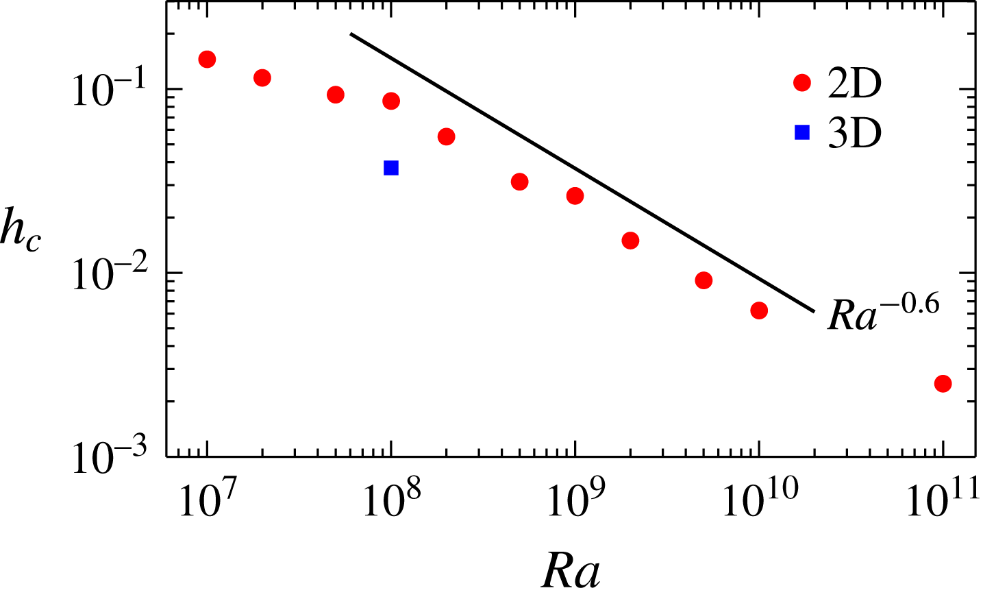
It is clear that the critical
 $h_{c}$
is different for different values of
 $Ra$
, i.e.
 $h_{c}$
decreases with increasing
 $Ra$
, as shown in figure 6. The question relates to which parameter in the system determines this critical roughness height
 $h_{c}$
. To quantitatively understand this dependence, we note that the fluid inside the cavity regions is mainly subject to two forces, i.e. the viscous force,
 $\unicode[STIX]{x1D708}U/h_{c}^{2}$
, due to the viscosity of the fluid, and the inertial force,
 $U^{2}/h_{c}$
, connected to the secondary flow in the cavities, where
 $U$
is the typical velocity of the LSC. When the roughness height
 $h$
(and the interspace) is small (or for small
 $Ra$
), the viscous force is dominant and the hot/cold fluid inside the cavity regions cannot be well mixed, thus resulting in a reduction of
 $Nu$
. On the other hand, for large roughness height
 $h$
(or for high
 $Ra$
), the inertial force becomes strong enough to generate smaller vortices, which leads to the strong mixing in the cavity regions (see also (Zhu et al.
Reference Zhu, Stevens, Verzicco and Lohse2017)) and correspondingly enhances the heat-exchange efficiency of the system. Therefore, at the critical roughness height
 $h_{c}$
, one should expect a balance between the two forces, i.e.
 $\unicode[STIX]{x1D708}U/h_{c}^{2}\sim U^{2}/h_{c}$
. We hence obtain
 $h_{c}\sim \unicode[STIX]{x1D708}/U=Re^{-1}$
. According to previous results of
 $Re\sim Ra^{0.6}$
in 2D RB flows (Sugiyama et al.
Reference Sugiyama, Calzavarini, Grossmann and Lohse2009; Zhang, Zhou & Sun Reference Zhang, Zhou and Sun2017), this yields
 $h_{c}\sim Ra^{-0.6}$
, which correctly reflects the trend in figure 6, at least within the range of
 $10^{8}\leqslant Ra\leqslant 10^{10}$
.
Log–log plot of
 $h_{c}$
as a function of
 $Ra$
for 2D (red circles) simulations. The solid line marks the scaling
 $Ra^{-0.6}$
for reference. For comparison, the value of
 $h_{c}$
obtained at
 $Ra=10^{8}$
in 3D cases is also plotted (blue square).

4 Conclusion
In summary, we have demonstrated that roughness does not always cause a heat-transfer enhancement. When the roughness height
 $h$
is small or
 $Ra$
is low, the hot/cold fluid can be trapped inside the cavities between the rough elements, thicken the thermal BL in these regions and consequently suppress the global heat transport through the RB system. The present results suggest that special care should be taken when applying rough surfaces to enhance the convective heat transfer.
The viscous effects become more important as
 $Pr$
increases or
 $Ra$
decreases, which would lead to an increase of
 $h_{c}$
. This is consistent with our dimensional arguments, i.e.
 $h_{c}\sim Re^{-1}$
, as previous numerical studies have shown that
 $Re$
decreases with increasing
 $Pr$
or with decreasing
 $Ra$
, for both 2D and 3D situations (van der Poel, Stevens & Lohse Reference van der Poel, Stevens and Lohse2013). In particular, for very small
 $Pr$
or for very large
 $Ra$
,
 $h_{c}$
should be too small to observe the
 $Nu$
reduction. On the other hand, for large enough
 $Pr$
or for small enough
 $Ra$
, very large
 $h_{c}$
is required to enhance the global heat transport. Due to the limitation of the cell height, however, heat-transport enhancement may not be achieved by surface roughness in this situation.
It should be noted that due to the lack of fluid motion in the third direction, the hot/cold fluid is more easily trapped within the cavity regions in two dimensions. This would result in a more pronounced
 $Nu$
reduction and a larger
 $h_{c}$
in the 2D simulations compared with those in the 3D simulations, as one can see in figures 2 and 6. It should also be noted that in most previous experimental studies, like that of Du & Tong (Reference Du and Tong1998), no
 $Nu$
reduction was observed in rough cells. This may be attributed to the different configurations of the rough elements. For example, Du & Tong (Reference Du and Tong1998) adopted pyramids as the rough elements, which have a convex geometry that can hardly trap the hot/cold fluid, while in our present study, a concave surface was chosen as the rough configuration (see figure 1
b). The concave rough surfaces make it possible for the hot/cold fluid to be trapped or accumulated inside the cavity regions, which should be the origination of the observed
 $Nu$
reduction.
Acknowledgement
This work was supported by Natural Science Foundation of China under grant nos 11572185, 11672156, 11732010 and 11772362.
Supplementary movie
Supplementary movie is available at https://doi.org/10.1017/jfm.2017.786.