Introduction
Reproductive frost damage has been estimated to cost Australian grain growers approximately A$360 m in direct and indirect yield losses annually (Baxter, Reference Baxter2015). These losses are most significant for wheat and barley, given their relatively low levels of tolerance to frost damage during flowering (Al-Issawi et al., Reference Al-Issawi, Rihan, El-Sarkassy and Fuller2013). Breeding new varieties with reduced frost susceptibility is one possible solution to this problem. Although genetic variation for frost tolerance during reproductive growth has been reported in barley (Reinheimer et al., Reference Reinheimer, Barr and Eglinton2004), the extent of genetic variation across all commercial wheat and barley cultivars remains unknown. This lack of knowledge has been partly a result of the practical difficulties in accurately measuring reproductive frost damage under field conditions due to the random and spatial variability of frost damage. Furthermore, the unpredictability of frost events (FEs) aligning with the most sensitive phase of reproductive development of wheat and barley has also proved challenging.
In contrast to grain yield, statistical design and analysis methods specific to the prediction of a variety's genetic propensity to tolerate frost, hereafter referred to as frost value, have been far less extensively researched. Like many grain quality traits in wheat, determining a variety's frost value is a complex process. This is due to issues such as low heritability, difficulty in determining an appropriate phenotype to measure, developmental differences between varieties at the time of a FE and the unpredictability of when a FE will occur and its severity. The duration and interaction with other microclimate factors suggests that frost damage is not consistent across each event. Screening for frost risk in Australia is the primary objective of a project funded by the Grains Research and Development Corporation, known as the Australian National Frost Project. This project operated from 2012 to 2016 and has since been replaced by a new project with similar aims: Screening for Frost Tolerance in Cereals. A key component of these projects is to conduct field experiments to investigate the frost value of a range of commercial and advanced varieties of wheat and barley.
The key trait which is related to reproductive frost damage is the so-called frost-induced sterility (FIS) of the plant head (Reinheimer et al., Reference Reinheimer, Barr and Eglinton2004); FIS is simply the ratio of sterile florets to total florets on per head basis. To maximize yield potential, commercial wheat crops are sown in autumn, which typically results in the plants flowering during late winter (barley) or early spring (wheat). Typically, wheat and barley have sufficient cold tolerance in their vegetative stages of development (SOD) to survive the relatively mild winters in Australia. However, when they transit into the reproductive stages during spring, the temperature overnight can still drop low enough over a prolonged period of time to cause a FE and thus potential FIS at this vulnerable SOD.
The level of sensitivity to frost is thought to continue to increase as the spike emerges from the boot and begins to undergo flowering (Frederiks et al., Reference Frederiks, Christopher, Sutherland and Borrell2015). The experimental phenotyping methodology implemented in the current project was based on that of Reinheimer et al. (Reference Reinheimer, Barr and Eglinton2004) and involved multiple sowing dates as separate field blocks at approximately equidistant thermal time. The strategy of multiple sowing dates was implemented to increase the likelihood that varieties would be at the booting (growth stage [GS] 49) or flowering (GS65) SOD (Zadoks et al., Reference Zadoks, Chang and Konzak1974), i.e. susceptible to damage when a FE occurred. Furthermore, it enables varieties of dissimilar maturity to be compared at the same SOD for a given FE. The samples of tillers that have heads at the appropriate SOD are tagged for a given FE and FIS is measured 4–6 weeks later in the laboratory once the plant has developed and achieved grain set (~GS85). This is required to distinguish between viable and sterile florets and thus exposure to multiple FEs is unavoidable, where FIS is a combination of both frost damage to anthers and ovules at or around flowering (GS65) and developing grains (GS70–79). Separation of the aborted anthers/ovules from frosted grains would require tedious dissection. Therefore, the presence or absence is recorded on frozen samples which indicate if a whole grain is present or absent at ~GS85. This process is repeated for all successive FEs, where some tillers may be tagged more than once if they are at two different SOD for separate events. This protocol results in a highly unbalanced longitudinal experiment (Brien and Demetrio, Reference Brien and Demetrio2009), in which there is potentially unequal sampling of each field plot in the experiment for each FE.
Smith et al. (Reference Smith, Ganesalingam, Kuchel and Cullis2015) and subsequently Gogel et al. (Reference Gogel, Smith and Cullis2018) described an approach to the analysis of yield data from crop variety evaluation programmes, where variety trials across years and locations are collated into a multi-environment trial (MET) dataset. Their approaches are based on the factor analytic (FA)-mixed model of Smith et al. (Reference Smith, Cullis and Thompson2001) and demonstrate the utility of this approach in terms of reporting results at a local or grower level. In the current paper, the Smith et al. (Reference Smith, Ganesalingam, Kuchel and Cullis2015) and Gogel et al. (Reference Gogel, Smith and Cullis2018) approaches for yield data from standard METs are extended for FIS data from frost expression experiments (FEEs). As such, the extension involves accommodation of longitudinal data and highly unbalanced nested designs within individual FEEs. Additionally, Smith and Cullis (Reference Smith and Cullis2018) developed a set of summary tools in the context of plant breeding selections for early stage yield evaluation trials. These tools can be generalized to all MET analyses in the FA-mixed model paradigm and can be applied in the context of the FEE analysis. The results from the analysis can therefore be summarized not only at the grower level but also for breeders to identify and explore the genetic composition of varieties that have lower frost risk than others.
The current paper is organized as follows: in ‘Materials and methods’ section the measurement protocol for a FEE is outlined, followed by a hypothetical example of a balanced FEE. An analysis of variance (ANOVA) approach derived from the hypothetical FEE is then extended to the linear mixed model (LMM) framework to accommodate the sparsity of FEEs and the subsequent MET analysis of all 17 FEEs. The model fitting process and tools for interpreting the final fitted model are also described. The results for the final fitted model to the MET dataset and methods developed to summarize information on frost risk for growers and breeders are presented in ‘Results’ section. ‘Discussion’ section provides a summary of the tools described in ‘Results’ section and describes their impact on the choices to be made by both growers and breeders. A glossary of acronyms used throughout the paper is given in Table 1.
Glossary of the most frequently used acronyms throughout the paper

Materials and methods
The FEEs in the MET dataset for the current paper were established in three states (New South Wales [NSW], South Australia [SA] and Western Australia [WA]) from 2012 to 2016 inclusive. The locations used included Narrabri (NSW), Loxton (SA), Brookton (WA), Merredin (WA) and Wickepin (WA). Two additional FEEs were sown in 2010 and 2011 at Loxton and were included in the MET dataset, as many varieties in these trials were the same as those in 2012–2016 and were grown using the same or similar designs and measurement protocols.
Measurement protocol
It is known that the susceptibility to frost damage increases with plant maturity (Al-Issawi et al., Reference Al-Issawi, Rihan, El-Sarkassy and Fuller2013): the anthers within florets are particularly sensitive to frost damage. In the case of sterile anthers due to frost damage, this process is not initiated and so the number of grains that are formed and viable for harvest is less than the total number of expected grains for that particular head. Pollen development begins while the spike is still contained within the boot and the sensitivity to cold damage increases during pollen meiosis (Barton et al., Reference Barton, Cantrill, Law, Phillips, Sutton and Overall2014). As a result, the protocol for these FEEs stipulates that the plants be tagged at the booting or flowering stage(s) of development following a FE to capture the range in susceptibility over time.
The trait measured (i.e. FIS) is used to derive the genetic response of interest (frost value), which depends on the definition of a so-called FE. Here a FE was defined by the canopy temperature of a trial falling to 0 °C or below. Tillers were tagged if they were at a susceptible SOD i.e. flowering or booting, within (i.e. ±) 48 h of a FE. Hence, the SOD of each (sampled) tiller was recorded for each FE.
Ancillary biotic data were also recorded either at the field plot or tiller level. All field plot measurements are taken on templated tillers, where a templated tiller is defined to be a single tiller in a field plot chosen to reflect the cohort of remaining tillers tagged for a defined SOD. The set of field plot level measurements included the percent of tillers within a field plot at the same SOD as the template (hereafter referred to PercentPlotStage); height of the templated tiller (hereafter referred to as Height); the distance from the flag leaf collar to the base of the spike on the templated tiller (PeduncleLength); the name of the technician who tagged the tillers in a plot for a given FE (hereafter referred to as Tagger). The measurements that were collected at the tiller level are the total number of seeds in the head of the plant (TotalNumberOfSeeds), total number of sterile seeds in the head (NumberOfSterileSeeds); the length of the spike on the tagged tiller (hereafter referred to as Length); the name of the technician who counted the total number of seeds and sterile seeds in the head of the tiller (hereafter referred to as Counter). Taggers and Counters are considered due to the subjective nature of their measurements and to more accurately estimate the genetic variance by taking into account all possible non-genetic sources of variation.
There are a number of unique growth stages recorded at tagging. The unique identifiers of growth stage at tagging are ear emergence, booting, flowering and not recorded. The latter encompasses stages that are synonymous with cases where FIS has been recorded outside the sampling protocol, i.e. tillers sampled at random throughout the course of the experiment or tagged at a different SOD to those pre-specified in the protocol. FIS records for tagged tillers that are classified as ‘not recorded’ cannot be included in the statistical analysis and are therefore removed from the final dataset. For the purpose of analysis, the remaining SOD were then reduced to two stages, namely flowering and booting, where the latter encompasses both the stages of booting and ear emergence. Further data cleaning was undertaken to remove data records where FIS exceeded one and/or the total number of floret positions was <10 or >60, as these were regarded as either unreliable or unreasonable measurements.
Experimental design
To facilitate the explanation of the experimental design, a hypothetical and simple FEE is considered in which there are three times of sowing (TOS) and six varieties. This scenario is presented in Fig. 1, where each of the field blocks is not necessarily spatially adjacent. In this example, each block comprises two sub-blocks with six field plots in each. The field plots in Fig. 1 with an ‘X’ are those with FIS data recorded over the course of the experiment and will be addressed below.
(Colour online) Field layout of a hypothetical FEE with three TOS and six varieties. Each of the three field blocks contain two sub-blocks and six field plots per sub-block. The ‘X’ indicates that FIS data were recorded for tillers within that plot.

In the design of an FEE, the treatments are the combinations of TOS and variety. Each TOS is assigned to a whole block and each of the six varieties is randomized to field plots within sub-blocks, such that the sub-blocks within a block are resolvable with respect to varieties. Thus, this allocation of treatments to plots results in a nested design that is similar to a split-plot design (see Bailey, Reference Bailey2008 Chapter 1, p. 131 for a discussion).
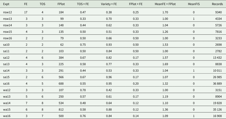
The FIS data collected from these FEEs (Fig. 1) are sparse and therefore the number of TOS, field plots and varieties sampled (i.e. that data exist for) is often not the total number for each of these factors in the designed experiment. In other words, the total number of TOS in Fig. 1 is three but the number of TOS for which there is FIS data is two. Table 2 presents a summary of key features of the real MET dataset.
Summary of the total number of FEs, time of sowing (TOS) and field plots (FPlot) sampled for each of the 17 FEEs in the MET dataset. A measure of sparsity is also provided for TOS × FE, Variety × FE and FPlot × FE combinations that exist, presented as a proportion of all possible combinations for each experiment. The mean number of FE for each FPlot, mean FIS and total number of data records are also summarized for each experiment in the MET dataset
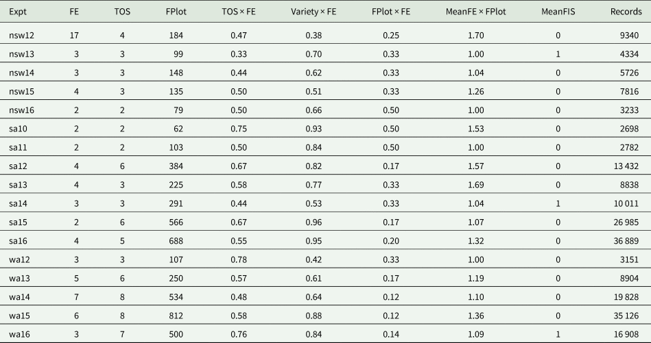
The number of FEs for each of the FEEs varied from 2 to 17 (nsw12), while the number of TOS sampled ranged from two to eight. The total number of plots sampled also varied markedly between FEEs and there was a significant degree of sparsity in the data at the TOS (TOS × FE), variety (Variety × FE) and field plot by FE (FPlot × FE) levels. It is clear that for four of the 17 FEEs (nsw13, nsw16, sa11 and wa12), all sampled field plots were unique to a single FE, whereas 70% of all field plots with data in nsw12 were tagged for at least two of the 17 FEs that occurred. The severity of FIS also varied substantially between FEEs (MeanFIS), while the range in total number of observations for each FEE was 2698 (sa10) to 36 889 (sa16). Finally, with the exception of nsw16, sa10 and sa11, there were data records for both SOD for each of the FEEs, however only 14 of the 74 (18.9%) FEs across all 17 FEEs had tillers tagged at both SOD (data not shown).
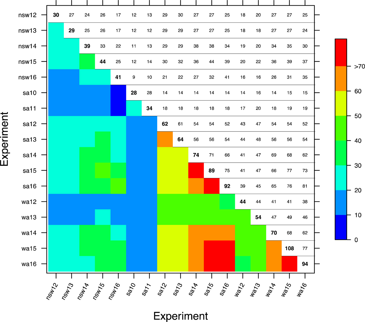
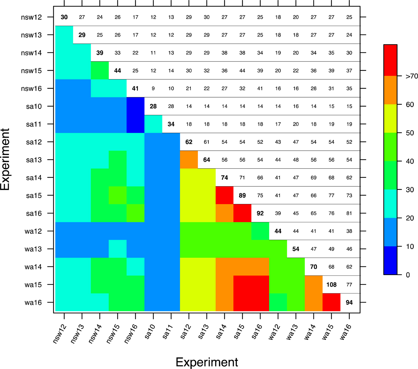
Figure 2 presents the variety connectivity matrix between the 17 FEEs in the MET dataset. The upper triangle presents the number of varieties in common between the pairs of FEEs, the lower triangle is a heat-map representation of the connectivity and the diagonals are the number of varieties that were sampled in each FEE. With the exception of sa10 and sa11 (which have a smaller number of unique varieties sampled), the connectivity between FEEs in general is quite reasonable (>20 varieties in common between pairs of FEEs) considering the stochastic nature of FEs and subsequent alignment with the required phenological development stages of the crop.
(Colour online) Connectivity of varieties for each of the 17 FEEs, where the number of varieties sampled at each trial are on the main diagonal and those in common between pairs of trials are presented on the off-diagonal.
Statistical methods
The MET approaches of Smith et al. (Reference Smith, Ganesalingam, Kuchel and Cullis2015) and Gogel et al. (Reference Gogel, Smith and Cullis2018) will be extended for the analysis of the FEE data. The analysis of the MET dataset needs to consider the aims of the experiment, the experiment design, the longitudinal nature of the data and the high degree of unbalance in the data within and between FEEs. The aim of the FEEs is to provide accurate frost value predictions for varieties. This requires formulation of an efficient and valid analysis which incorporates all sources of variation and accounts for dependence through the longitudinal structure of the data. This analysis is embedded within the framework of LMMs and therefore requires enumeration of the terms in the fixed and random model formulae, which will ensure the analysis is linked to classical or randomization-based analyses of comparative experiments (Bailey, Reference Bailey2008, p. 132).
A hypothetical and balanced FEE that can be analysed using ANOVA is initially considered in the interest of simplicity. A single FEE with one FE and SOD is presented first and then this is modified to accommodate multiple FEs and the two SOD for a single FEE. This is then extended to the LMM framework in section ‘LMM for the MET FEE dataset’ to accommodate the non-orthogonality of the data and to allow for the subsequent analysis of the MET dataset that satisfies the aims of the project. In the following development, the inclusion of ancillary data (described in section ‘Measurement protocol’) is only addressed in section 'LMM for the MET FEE dataset'.
Analysis of variance for a hypothetical and balanced frost expression experiment
Figure 1 presents the layout of a hypothetical FEE and will be used here as a motivating example for the real dataset. In this case, an ‘X’ is considered to be present in every field plot and it is assumed that eight tillers from each plot have FIS data recorded. As previously described, the treatments are combinations of the levels of TOS and variety. The observational units are the tagged tillers. The treatments are applied to the observational units such that (a) all tillers within a plot relate to the same variety, (b) each plot within a sub-block is allocated a different variety but the same TOS, (c) each sub-block within a block contains one replicate of each variety and a single TOS and (d) each block receives a different TOS. The plot and treatment structures for the hypothetical FEE using the notation of Wilkinson and Rogers (Reference Wilkinson and Rogers1973) are given as follows:


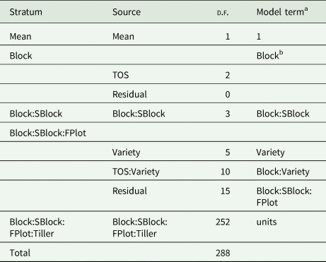
where the sub-blocks are denoted by SBlock and individual field plots by FPlot to distinguish the latter from the ‘plot’ structure. The factors are defined such that Block has three levels, SBlock has two levels, FPlot has six levels, Tiller has eight levels, TOS has three levels and Variety has six levels. The expansion of these two structures gives rise to the ANOVA (Table 3). This table has been augmented to include the model terms that would be fitted as an LMM surrogate for the ANOVA approach. Recall that each Block is representative of a different TOS and hence TOS is aliased with Block. This is clearly shown in Table 3 by the 0 d.f. associated with the Block stratum residual. Use of the correct plot structure in the ANOVA therefore guards against invalid inference on the main effects of TOS. Note that Table 3 shows there is a valid test for the interaction term labelled as TOS:Variety. However, given the aliasing of TOS and Block and the fact that the sowing times are not randomized to blocks but rather applied in a convenient and systematic order, it is not justifiable to conclude that the interaction effects are associated with TOS alone. In terms of the surrogate LMM, the aliasing requires a choice of factor name (i.e. Block or TOS). In the Model Term column of Table 3 all instances of TOS have been replaced by Block to avoid inferences being made on TOS.
ANOVA for a hypothetical FEE with a single FE
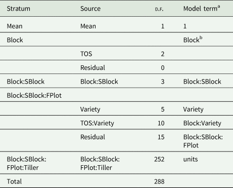
d.f., degrees of freedom; TOS, time of sowing; SBlock, sub-block; FPlot, field plot.
a The model term column has been included to represent the terms fitted for a LMM surrogate for the ANOVA approach. Note that 1 is representative of the overall mean and units is synonymous with the observational units in the LMM package ASReml.
b TOS and Block are aliased and therefore all instances of TOS are replaced with Block in the LMM.
This scenario is now extended to the case of multiple FEs and the two SOD over the course of a FEE. For this example, it is assumed that eight different tillers in each plot are tagged at three times, making a total of 24 observational units per plot. It is also assumed that of the eight tillers tagged per plot, there are four at each of the two pre-specified SOD. SOD is a factor that has not been applied/randomized but has effects, including interactions with the treatment factors that are of interest to researchers. Time is considered here to be a longitudinal factor and following Brien and Demetrio (Reference Brien and Demetrio2009), it is crossed with the plot factors that are potentially involved in the repeated measurement process i.e. Block, SBlock and FPlot but not Tiller. The cohort of tillers tagged for the same FE and subsequent interactions with the remaining treatment factors are also of interest and can be accounted for by the inclusion of Time in the treatment structure. The plot and treatment structures for the hypothetical FEE with multiple FEs and SOD are given as follows:


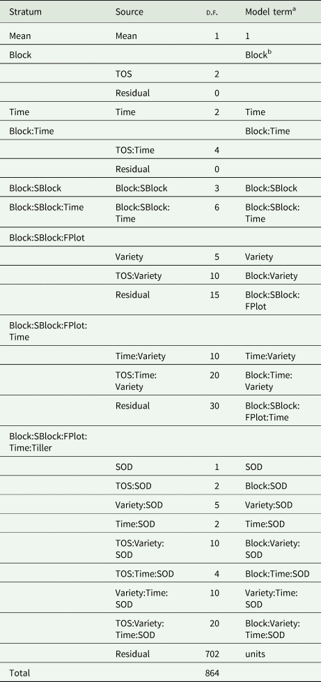
The factor Time has three levels and SOD has two levels in this example, where all other factor levels remain unchanged. The ANOVA for an orthogonal FEE with multiple FEs is given in Table 4 where the LMM surrogate is again indicated using the Model Term column.
ANOVA for a hypothetical FEE with multiple FEs and SOD

d.f., degrees of freedom; TOS, time of sowing; SBlock, sub-block; FPlot, field plot.
a The model term column has been included to represent the terms fitted for a LMM surrogate for the ANOVA approach. Note that 1 is representative of the overall mean and units are synonymous with the observational units in the LMM package ASReml.
b TOS and Block are aliased and therefore all instances of TOS are replaced with Block in the LMM.
Linear mixed model for the multi-environment trial frost expression experiment dataset
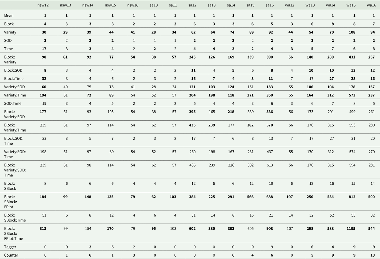
The hypothetical FEE described above was for a completely balanced and orthogonal experiment. Table 5 presents a summary of key features of the MET dataset for the 17 FEEs that captures the sparsity in the dataset as a direct result of the measurement protocol that was implemented. The LMM as derived by Smith et al. (Reference Smith, Ganesalingam, Kuchel and Cullis2015) and Gogel et al. (Reference Gogel, Smith and Cullis2018) thus provides a natural framework for the analysis of such experiments as an ANOVA analysis is not feasible. In the current paper, a general LMM that removes any restrictions concerning orthogonality of block structures is proposed by extension of the model specified in Table 4. This allows modification of the fixed and random model specifications to satisfy the aims of the experiment, capture additional sources of non-genetic variation and include factors of interest to the researcher.
Number of levels associated with each term in the LMM for each of the 17 FEEs

SOD, stages of development; SBlock, sub-block; FPlot, field plot.
Also note that those in bold were fitted for each of the respective FEEs in the MET analysis.
In the following derivation, the data are ordered as observational units within each of the 17 FEEs (Expt). Formulation of the plot structure for the MET dataset is a simple extension of the plot structure derived in Table 4. All model terms in the plot structure are now nested within Expt as each of their respective levels and interactions are unique to each FEE. The treatment structure for the MET dataset, however, is quite complex. In a MET analysis, there is particular interest in modelling and accounting for variety by environment interaction (VEI), to examine and exploit the set of environmental conditions experienced by each FEE. Additionally, there are at least nine or more varieties that are in common between each of the 17 FEEs (Fig. 2). Therefore, both Variety and SOD are crossed with Expt as both the main effects and interactions of these terms are meaningful and consistent across the MET dataset. Each Time however, is unique to (nested within) each Expt and therefore its levels are not consistent across all FEEs. Similarly, the levels of TOS are also nested within Expt as each TOS is not only aliased with Block but they are also inconsistent across the 17 FEEs. The resulting plot and treatment structures for the MET dataset are given by


Given the sparsity of the data collected, it is not possible to fit the full LMM that results from the expansion of the above structures. Table 5 presents a summary of the number of levels associated with each term in the maximal single site mixed model for each FEE. The numbers in bold indicate that the corresponding term can be and was fitted in the LMM for that FEE. Of particular interest is the lack of information on Variety:SOD for most FEEs which will be discussed further in the results. All remaining terms in the table that are not bold were excluded for an FEE due to either structural aliasing or implicit aliasing with another term(s). This was determined by using an algorithm designed to detect singularities in the average information matrix to identify aliasing of fixed and random effects that were not already explicit but attributed to the sparsity in the data. The details of this approach are not presented.
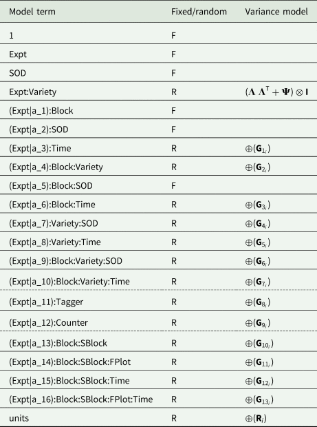
The LMM presented in Table 6 was the final model fitted to the FEE MET dataset. Following Bailey (Reference Bailey2008, p. 14), the treatment structure is initially fitted as fixed and the plot structure as random in the LMM. To guard against invalid inferences being made, particularly for the effects of TOS, all instances of TOS were replaced with Block as also shown in Tables 3 and 4. The main effects of Expt and Time are present in the expansion of both the plot and treatment structures. The main effects of Time and all interactions with Time were fitted as random effects in the LMM. This is due to the fact that tagged tillers may be exposed to multiple FEs so that each time is not necessarily representative of a single FE but instead represents the cohort of tagged tillers at that time. The main effects of Expt were fitted as fixed for reasons outlined below.
Final LMM for the FEE MET dataset

TOS, time of sowing; SOD, stages of development; SBlock, sub-block; FPlot, field plot.
The expansion of the treatment and plot structures and the additional sources of extraneous variation are separated by the dashed lines. Note that all instances of TOS are replaced with Block as the two terms are aliased.
The aim of the analysis is to determine the frost value of each variety and thus rank their relative risk to frost. Therefore best linear unbiased predictors are preferable over best linear unbiased estimates as the probability of selection errors are minimized under the former approach (Bueno Filho and Gilmour, Reference Bueno Filho and Gilmour2007). Thus, the main effect of Variety and all interactions with Variety were fitted as random effects in the LMM in Table 6. The main effects of Expt were fitted as fixed effects to provide appropriate mean values for estimation of the genetic and residual variance structures. Other terms that may be potential sources of variation (and not genetically determined) and are not necessarily of interest (Diggle and Chetwynd, Reference Diggle and Chetwynd2011) are also considered here. In this setting, these would include the people who have tagged the individual tillers (Tagger) and those who counted the sterile and total numbers of grains in each head (Counter). Tagger and Counter are assumed to be unique to each of the individual FEEs and therefore the levels associated with each are nested within Expt.
There are many characteristics of Table 6 that require explanation and defining. Firstly, for any terms where the prefix Expt|a_j, j = 1,2,…,16 is fitted, the levels contained in a_j are the names of those FEEs for which that term must be fitted and is hereafter called a conditioned factor. There are a total of 16 conditioned factors in Table 6, where SOD for example will only be fitted for those 12 FEEs (bold in Table 5) listed in a_2, which are FEEs with data measured at both levels of SOD and that are not aliased with any other term.
The $\oplus$ operator represents a block diagonal variance structure, with each block corresponding to a separate FEE, i. For each ${\bf G}_{k_i}$
 , k = 1, 2, …, 13 in Table 6, the variance matrix is given by ${\bf G}_{k_i} = \sigma _{k_i}^2 {\bf I}_{b_{k_i}}$
 . In other words, for the ith FEE contained in a_j, a unique value of $\sigma _k^2$
 is calculated and for ease of presentation was not explicit in Table 6. For example, the variance model for the term (Expt|a_11):Tagger is $\oplus \lpar {\sigma_{8_i}^2 {\bf I}_{b_{8_i}}} \rpar$
 , where i now indexes each of the FEEs contained in a_11 and $b_{8_i}$
 is the dimension of ${\bf I}$
 that is equivalent to the total number of levels associated with Tagger for the ith FEE. Furthermore, the variance for the observational units of each FEE $(\oplus ({\bf R}_i))$
 , is a block diagonal matrix, where ${\bf R}_i = \sigma _i^2 {\bf I}_{b_i}$
 for i = 1, 2, …, 17 and the dimension b i is equal to the number of observational units for the ith FEE.
The expansion of the treatment structure included a main effect for varieties and an interaction term between variety and experiment. A more general variance structure can be obtained by excluding the Variety main effect from the model so that the term Expt:Variety no longer represents the interaction effects but rather the variety effects for each level of experiment, that is, the nested effects of varieties within experiment. The variance model for Expt:Variety is chosen to be a FA model after Smith et al. (Reference Smith, Ganesalingam, Kuchel and Cullis2015) and has been shown to provide a parsimonious model for VEI and also provide accurate predictions for the variety effects (Smith et al., Reference Smith, Ganesalingam, Kuchel and Cullis2015).
Using the notation of Smith et al. (Reference Smith, Ganesalingam, Kuchel and Cullis2015), the FA model of order k for the vector ${\bf u}$ of variety effects within environment (FEE) can be written as

where ${\bf \lambda}$ is the t vector of loadings, ${\bf f}$
 is the mk vector of scores, ${\bf \delta}$
 is the mt vector of genetic regression residuals, ${\bf I}$
 is an m × m identity matrix, t = 17 is the number of environments and m = 167 is the number of varieties in the full MET dataset. The variance matrices for ${\bf f}$
 and ${\bf \delta}$
 are Var$\lpar {\bf f} \rpar = {\bf I}_{mk}$
 and Var$\lpar {\bf \delta} \rpar = {\bf \Psi} \otimes {\bf I}_m$
 respectively, where ${\bf \Psi}$
 is a t × t diagonal matrix with a variance (called a specific variance) for each environment. Hence,

where ${\bf \Lambda}$ is the t × k matrix of loadings and ${\bf G}_{\bf e} = \lpar {{\bf \Lambda} {\bf \Lambda}^{\rm T} + {\bf \Psi}} \rpar$
 is defined to be the between environment genetic variance matrix.
Model fitting and tools for interpretation
All models in the current paper were fitted using the ASReml-R package (Butler et al., Reference Butler, Cullis, Gilmour, Gogel and Thompson2017) in the R statistical computing environment (R Core Team, 2015). The variance parameters were estimated using residual maximum likelihood (REML). In the FA model, the variance parameters are the loadings and specific variances and the REML estimates of these are denoted by $\hat{\lambda} _{rj}$ and $\hat{\psi} _j$
 (r = 1, …, k;j = 1, …, 17). Note when k >1, ${\bf \Lambda}$
 is not unique so estimation requires imposition of constraints. The approach used in ASReml-R fixes the k(k − 1)/2 elements in the upper triangle of ${\hat{\bf \Lambda}}$
 to zero. Once the REML estimate of ${\bf \Lambda}$
 is available, the matrix ${\hat{\bf \Lambda}}$
 is rotated to the principal components solution (Smith et al., Reference Smith, Cullis and Thompson2001) and henceforth assume ${\hat{\bf \Lambda}}$
 relates to the rotated solution.
Given the set of REML estimates of the variance parameters, the empirical best linear unbiased predictors are obtained of the random effects for ${\bf f}$ and ${\bf \delta}$
 . These are denoted by $\tilde{f}_{ri}$
 and $\tilde{\delta} _{ij}$
 (r = 1, …, k;i = 1, …, 167;j = 1, …, 17). The model fitting process involved fitting a sequence of FA models with increasing order to the Expt:Variety term. Note that all other terms remain in the LMM during the FA modelling.
Subject to the parameter estimate, the model in Eqn (1) resembles a multiple regression in which there are k environmental covariates $({\hat{\bf \lambda}} _1, \ldots, {\hat{\bf \lambda}} _k)$ and for each covariate, each variety has a different slope that is given by the corresponding predicted score $\lpar {{\tilde{\bf f}}} \rpar$
 . The final term in Eqn (1) represents the residual or lack of fit of the regression model $({\bf \delta} {\rm )}$
 . The choice for k is determined by the data and may be based on likelihood ratio tests or information criteria. A pragmatic approach is used here as advocated by Smith et al. (Reference Smith, Ganesalingam, Kuchel and Cullis2015) and k is chosen such that the percentage of genetic variance accounted for by the regression part of the model captures sufficient VEI for this particular application. The percentage variance accounted for (%VAF) by factor r = 1, 2, …, k is defined as

where diag extracts the diagonal elements of its t × t symmetric matrix argument as a t-vector and ${\rm \oslash}$ is the vector element-wise division operator. Additional summaries across environments and factors are given by

These quantities are the mean contribution of factor r across environments, the variance accounted for by all factors for each environment and the mean variance accounted for by all factors across environments respectively.
Results
The folded power and power transformations suitable for proportionate data were investigated to consider additivity of the LMM and more appropriately satisfy the normality assumptions of the data vector ${\bf y}$ in the LMM. In a linear models framework this is achieved via maximum likelihood (Atkinson, Reference Atkinson1987). This was approximated in the LMM framework by making an adjustment to the residual likelihood using quantities that were readily available in ASReml-R (Cullis and Smith, Reference Cullis and Smith2019). A constant, c, was required to shift FIS values of zero and one to enable transformation of the data. A traditional value for this constant is 0.5/n, where n is the index of the binomial distribution. This is not always a suitable choice so several pragmatic values of c were considered, namely c = p0.5/n, where p = 1/4, 1/2, 1, 2 and 4. The value of n used was the median total number of seeds across the dataset (n = 28). The adjusted profile likelihood approach for λ led to the choice of a folded power transformation with λ = 0, which corresponds to a logit transformation. In terms of the choice of c, the likelihood approach was combined with the use of diagnostic plots (Lee et al., Reference Lee, Nelder and Pawitan2006) resulting in the choice of p = 1/4, and thence c = 1/224. The data vector used for analysis is therefore given by

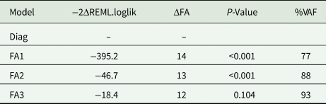
Initially, a baseline diagonal variance model (Diag) was fitted for the Expt:Variety effects, which is equivalent to analysing each of the 17 FEEs independently of one another. It was determined from this preliminary analysis that there was no genetic variance at the sa11, sa14 and wa16 sites (due to severe or no frost damage of all varieties) and so these trials were dropped from the subsequent MET analyses. The MET analysis of the remaining 14 FEEs consisted of fitting a series of FA models of increasing order k to the Expt:Variety effects. The REML log-likelihood test statistic (− 2ΔREML.loglik), difference in the number of FA parameters (ΔFA) for each model compared to its predecessor, P value associated with the REML log-likelihood ratio test (REML-LRT) for each model compared to its predecessor and %VAF (i.e. $\bar{v}_{\cdot}$ from Eqn (2)) by each model are presented in Table 7. It is clear that the FA1 model is superior to the Diag model (− 2ΔREML.loglik = 395.2), where the REML-LRT returned a P ≪ 0.001. The increase in REML.loglik between the FA2 and FA1 models was also shown to be statistically significant (P < 0.001, − 2ΔREML.loglik = 46.7). The higher order FA3 model was not found to be statistically significant compared to the FA2 model (P = 0.10), however the %VAF was substantially higher (93% compared to 88%) reflecting the capture of VEI that may be important for the provision of local grower information. Therefore, the results from the FA3 model were used for the frost value predictions of the unique varieties grown across the 14 FEEs.
Summary of variance models fitted to the Expt:Variety effects (Diag, FA1, FA2 and FA3) including the REML log-likelihood test statistic (− 2ΔREML.loglik), increase in number of FA parameters fitted (ΔFA), P-value associated with the REML log-likelihood ratio test of the current model to the one above and %VAF

REML, residual maximum likelihood; FA, factor analysis; %VAF, percentage variance accounted for.
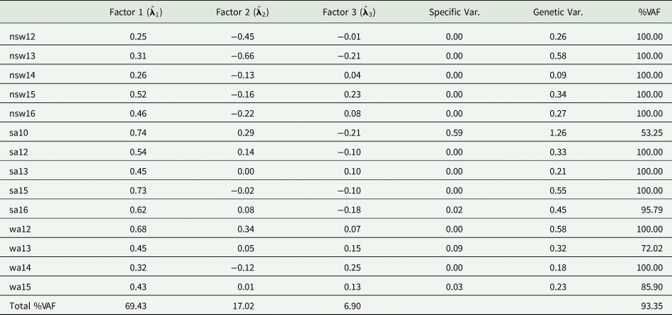
Table 8 presents the REML estimates of the (rotated) factor loadings, site specific variance and total genetic variance for each of the 14 FEEs from the fitted FA3 variance model. The %VAF for each site is given in the final column and the total %VAF by each of the three factors and across all FEEs is given in the final row of Table 8. The %VAF by the fitted model for each FEE was greater than 85%, with the exception of sa10 and wa13 with 53% and 72% %VAF respectively. The estimated loadings and specific variance were used to form the REML estimate of the between environment genetic variance matrix (denoted by ${\hat{\bf G}}_{\bf e}$ ). The diagonal elements of ${\hat{\bf G}}_{\bf e}$
 are the estimated genetic variance for individual FEEs and are given in Table 8. There is substantial heterogeneity across FEEs, with the estimated genetic variance ranging from 0.09 (nsw14) to 1.26 (sa10). Estimates of the between-environment genetic correlations can be obtained from ${\hat{\bf G}}_{\bf e}$
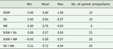
 and are summarized on a state basis in Table 9. This table shows that there is substantial VEI between FEEs in NSW and SA (minimum correlation of 0.09 between nsw13 and sa10) and between sites in NSW and WA (minimum correlation of −0.05 between nsw13 and wa12). The minimum estimated genetic correlations are much higher (indicating less VEI) between FEEs within the same state than across states.
REML variance estimates of the three (rotated) factor loadings $({\hat{\bf \lambda}} _j)$ , specific variance, total genetic variance and the total variance accounted for (%VAF) for each of the 14 FEEs for the FA3 variance model

REML, residual maximum likelihood; %VAF, percentage variance accounted for; FEEs, frost expression experiments.
The total %VAF for each of the three loadings and across all 14 FEEs is also given.
Summary of REML estimates of genetic correlations between pairs of FEEs within states and between states for the 14 FEEs in the MET dataset

REML, residual maximum likelihood; FEEs, frost expression experiments; NSW, New South Wales; SA, South Australia; WA, Western Australia.
The total number of paired comparisons is given as the final column.
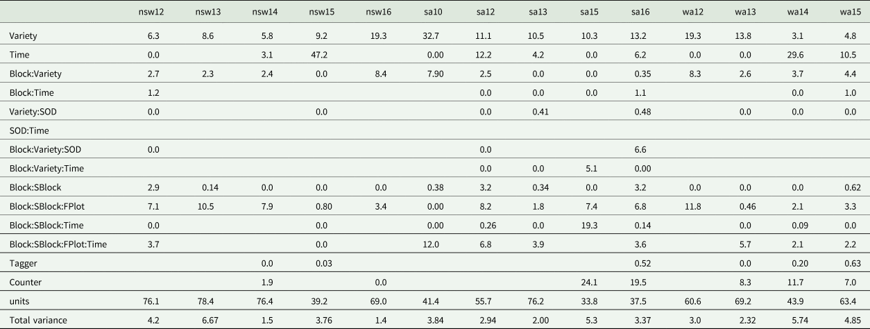
Table 10 presents the REML estimates of variance parameters from the FA3 model on an individual experiment basis, expressed as a percentage of the total variance for that experiment. These correspond to the Random Model Terms as listed in Table 6. A key feature of MET analyses requires variance modelling of all random terms and from Tables 8 and 10 it is clear that there exists variance heterogeneity at both the residual and genetic levels. Therefore, fitting Expt as a random model term would not permit this heterogeneity to be properly accounted for. The genetic variance attributable to variety effects for each experiment (diagonal elements of ${\hat{\bf G}}_{\bf e}$ ) accounted for between 3.12% (wa14) to 32.73% (sa10) of the total variance of each experiment. All other sources of genetic variation within FEEs, that is, interactions between Variety and Block (TOS), Time and SOD were much smaller (where able to be fitted). Thus it was valid to confine the reporting of grower information to Expt:Variety predictions. Additionally, this is supporting evidence for the choice of relatively simple variance structures for the genetic terms other than Expt:Variety. The large contribution of the units term (ranging from 33.76% to 78.38%) was expected since this is a difficult trait to measure and between tiller variation is inevitable. We note however, that the protocol addresses this issue by ensuring large numbers of tillers within plots for a given FE (mean of 33) are sampled. Thus the impact of the large between tiller variation on standard errors for variety predictions is mitigated due to division by such large numbers.
Percent variance associated with the random model effects in the LMM for each of the 14 FEEs

LMM, linear mixed model; FEEs, frost expression experiments; SOD, stages of development; SBlock, sub-block; FPlot, field plot.
The total variance is also given and note that units is the syntax used in the LMM package ASReml to index the observational units in the model.
Selection of low frost risk varieties
The primary aim of the FEE MET analysis is to inform local growers of the relative frost susceptibility of commercial and advanced wheat varieties in a range of environments. The Production Value-PLUS (PV-PLUS) graphs introduced by Smith et al. (Reference Smith, Ganesalingam, Kuchel and Cullis2015) are an appropriate tool for summarizing variety performance at a level where growers can exploit the environmental conditions represented by individual FEEs and apply that information to their own farming systems. Given the nature of the analysis, it will also be possible to provide information that is of use to the breeders and researchers. Varieties that consistently demonstrate lower frost risk (high adaptation) or low risk in specific environments only (specific adaptation) are also of interest. The genetic predisposition of these highly and/or specifically adapted varieties can then be explored with the aim of introducing reduced susceptibility to frost in future breeding.
With this in mind, it would be sensible to initially use summary tools such as those presented in Smith and Cullis (Reference Smith and Cullis2018), which are based on the regression interpretation of the FA model as described in the section on model fitting and tools for interpretation. It is noted that the rotated environment loadings for the first factor of the fitted FA3 model are all positive (Table 8). This indicates that the VEI accounted for by the first factor is driven by scale. In other words, the rankings of each variety in reference to frost risk do not change across each environment (for the first factor); however, the magnitude of the differences between each variety may change, thus leading to scale VEI. It is therefore meaningful to then determine the so-called overall performance (OP) for each of the varieties using the fitted values in the regression for the first rotated factor, which are given by $\lpar {{{\hat{\bf \lambda}}}_1\otimes {\bf I}_m} \rpar {\tilde{\bf f}}_1$ (see Eqn (1)). Thus the OP for variety i is given by $\bar{\lambda} _1\tilde{f}_{1i}$
 , where $\bar{\lambda} _1 = (1/14)\sum\nolimits_{j = 1}^{14} {{\hat{\lambda}} _{1j}}$
 (Smith and Cullis, Reference Smith and Cullis2018).
The growers, breeders and researchers are also interested in measures of stability of frost value across FEEs. Smith and Cullis (Reference Smith and Cullis2018) provide a measure for FA models that is based on factors 2, …, k (i.e. excluding the first). It is based on the sum of squares of fitted values for the second and higher order regression terms and is referred to as root mean square deviation (RMSD). Both OP and RMSD are expressed in the units of measurement of the trait being analysed, in this case the transformed FIS value. Figure 3 illustrates the OP v. RMSD for the 159 varieties that were sown in the FEE MET dataset used for analysis on the scale of the (transformed) data. Those varieties with a low OP and RMSD are considered to be superior in the sense that they have low frost risk (concurrent with a low frost value) and are relatively stable across all 14 environments. Therefore, those varieties in the bottom left corner should be those of interest to particularly the breeders for low susceptibility to frost damage.
OP v. RMSD for frost values of all varieties sampled in the FEE MET dataset. Varieties in the bottom left corner are considered to be the least susceptible to frost and stable performing across all environments. Those varieties that were present in less than three FEEs appear more transparent than the remaining varieties present in three FEEs or more.
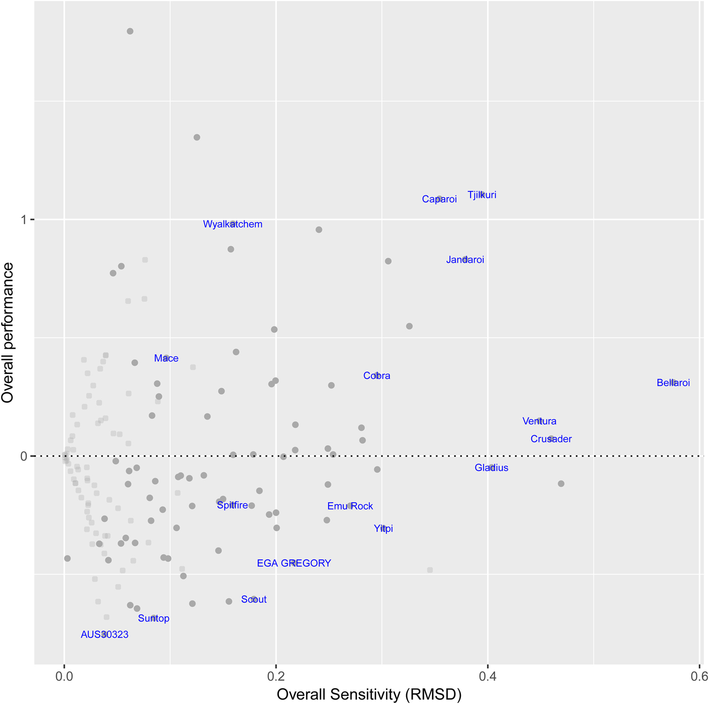
The points in Fig. 3 have been shaded lighter if that variety was grown in less than three of the possible 14 environments in the MET dataset. Although this is not an exact measure of the accuracy of OP, it cautions the user on interpretation of the OP for this set of varieties that were only grown in a minimal subset of the environments in the MET dataset. Figure 3 shows that the varieties AUS30323 and Suntop had low overall frost risk and were also very stable. The widely grown Wyalkatchem was one of the most frost susceptible varieties. The most unstable variety was Bellaroi. Four durum wheat varieties (Bellaroi, Caparoi, Jandaroi and Tjilkuri) were tested in the FEEs and all exhibited unstable performance with above average overall susceptibility (OP > 0).
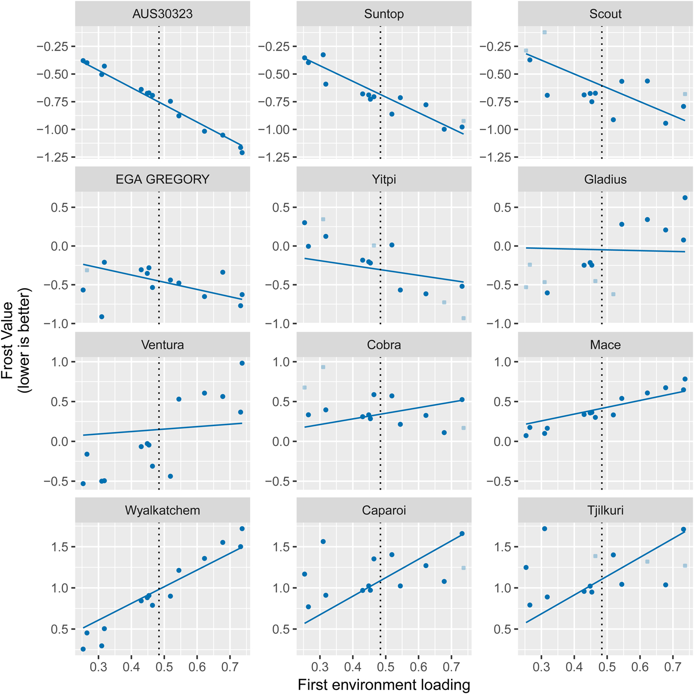
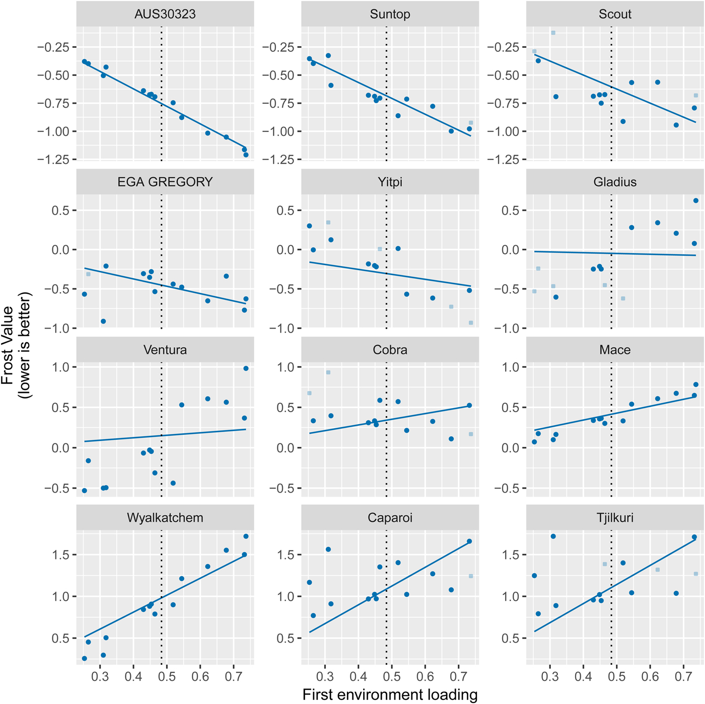
OP and RMSD are summary measures derived from the regression associated with the first set of loadings. It is instructive to visualize the entire regression using latent regression plots (Smith and Cullis, Reference Smith and Cullis2018) for varieties of interest. Figure 4 shows the latent regression plots for the first factor for 12 of the 17 varieties labelled in Fig. 3. The points on each graph are the common variety by environment effects (frost values), which are the predictions of the regression part of Eqn (1) (Smith and Cullis, Reference Smith and Cullis2018). Note that, for each variety in Fig. 4, OP is the value on the regression line at the mean value of the loadings (shown as the dotted vertical line) and RMSD is computed using the deviations of the points from the line. Of the lower risk varieties, the stability of AUS3023 and Suntop compared with Scout is clearly shown. Note that the instability of Scout has some positive aspects, since it exhibits a lower risk than AUS3023 and Suntop at some sites (in particular nsw15 and wa14). The instability of Ventura and the durum varieties is also clear in Fig. 4.
Latent regression plots of frost values for 12 varieties for the first factor only in the fitted FA3 variance model. The data-points are transparent to indicate a variety was not measured for FIS in a particular environment and note the change in frost value scale across the rows. The vertical dashed line is the mean value of the first factor loadings for all 14 environments.
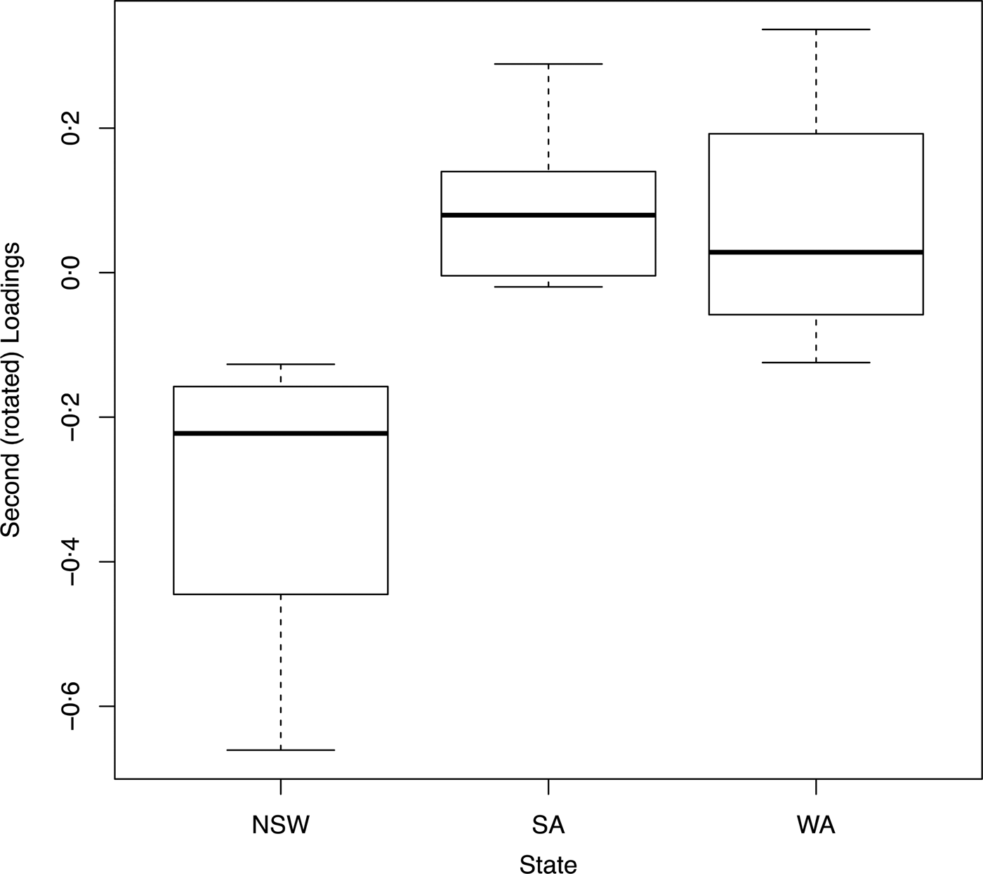
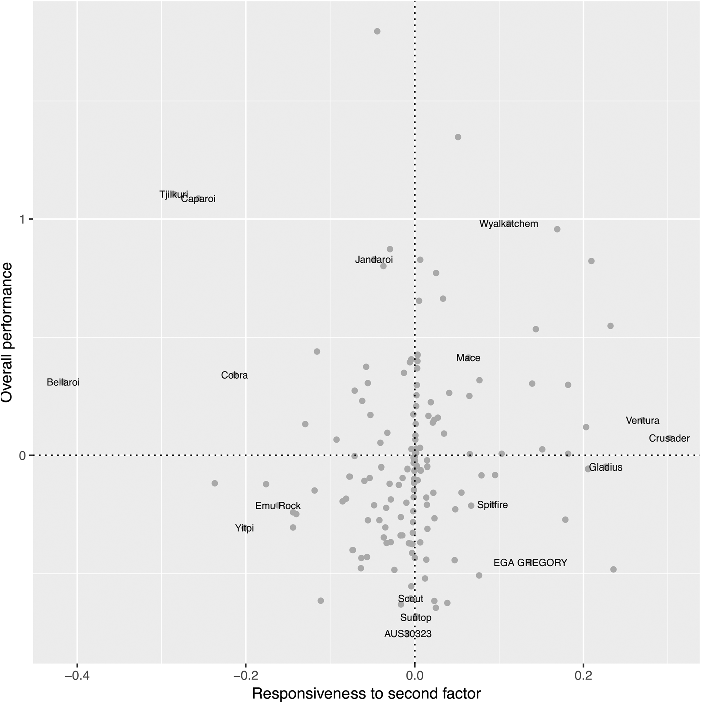
RMSD represents combined responsiveness to all factors other than the first. It may be helpful to consider the responsiveness to individual factors, particularly if the factor can be ascribed a meaningful interpretation. In the current example, the second factor largely represents a contrast between sites in NSW and the other two states. This can be seen using Table 8, but is more clearly illustrated in the box-plot in Fig. 5. This contrast aligns with prior knowledge in the sense that the impact of FEs in northern NSW (where the sites are located) is likely to differ from events in more southern and western growing regions. Also note that this is reflected in the summary of estimated genetic correlations in Table 9. The responsiveness to this factor for individual varieties (Smith and Cullis, Reference Smith and Cullis2018) is shown in Fig. 6. Of particular interest are Ventura, Crusader (which have large positive responses) and three of the durum varieties (Bellaroi, Caparoi and Tjilkuri) and Yitpi (which have large negative responses). This means that Yitpi and these durum varieties have relatively lower risk in SA and WA sites compared with NSW whereas for Ventura and Crusader, the opposite is true.
Box-plot of the second (rotated) loadings for each state (NSW, SA and WA) from the fitted FA3 genetic variance model.

OP v. responsiveness to the second (rotated) factor for frost values of all varieties sampled in the FEE MET dataset. Varieties that are close to the line x = 0 are considered to be non-responsive to the covariate(s) implicit in factor two.

Figures 3, 4 and 6 provide valuable information about varietal performance across the entire MET dataset. This is crucial for breeders and may also be of interest to growers. However, it is also pertinent that growers are provided with accurate and efficient estimation of performance that is relevant to their local area. The complexity of the VEI necessitates systems such as these to guide optimal selection decisions. For example, a variety that appears unstable may perform favourably and be specifically adapted to a particular growing region. The PV-PLUS graphs for the set of varieties that are commonly grown in NSW and SA only are presented (Figs 7 and 8).
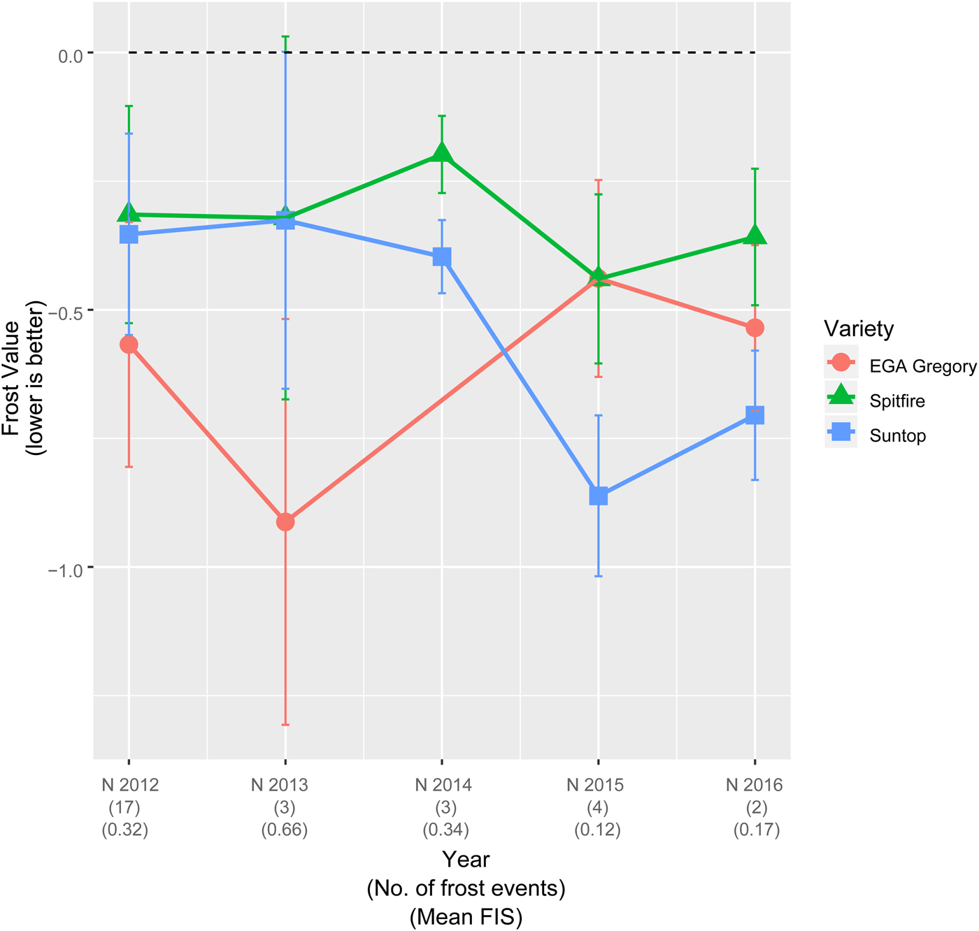
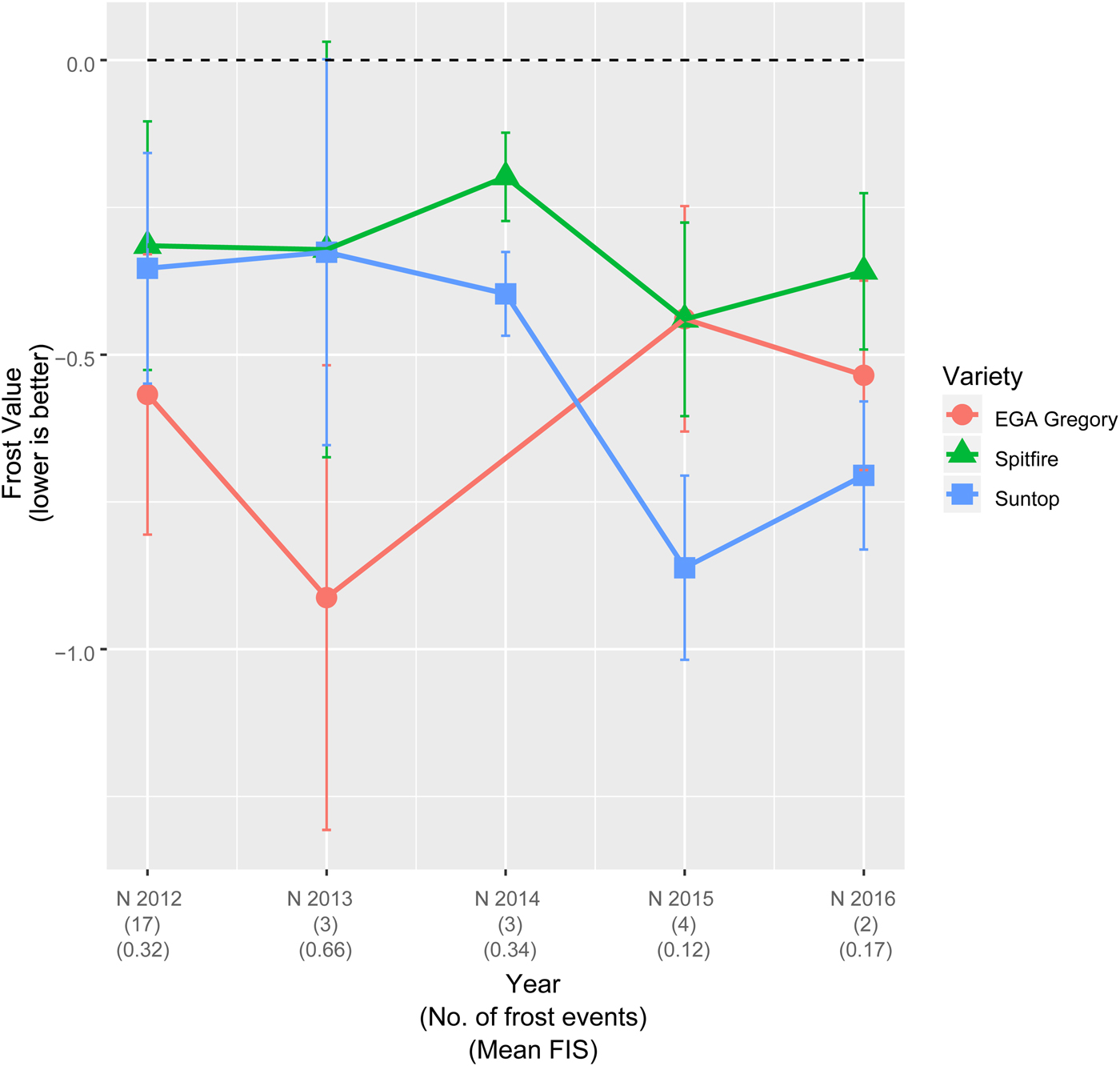
(Colour online) PV-PLUS plot for NSW. Each of the NSW FEEs from 2012 to 2016 are listed on the x-axis and the corresponding predicted frost value for each of the three varieties on the y-axis together with standard error bars. The number of FEs and mean FIS for each FEE is also presented underneath the experiment name. Predicted frost values are not presented for varieties that did not have FIS measured for a given FEE.
(Colour online) PV-PLUS plot for SA. Each of the SA FEEs from 2010 to 2016 are listed on the x-axis and the corresponding predicted frost value for each of the five varieties on the y-axis together with standard error bars. The number of FEs and mean FIS for each FEE is also presented underneath the experiment name. Predicted frost values are not presented for varieties that did not have FIS measured for a given FEE.
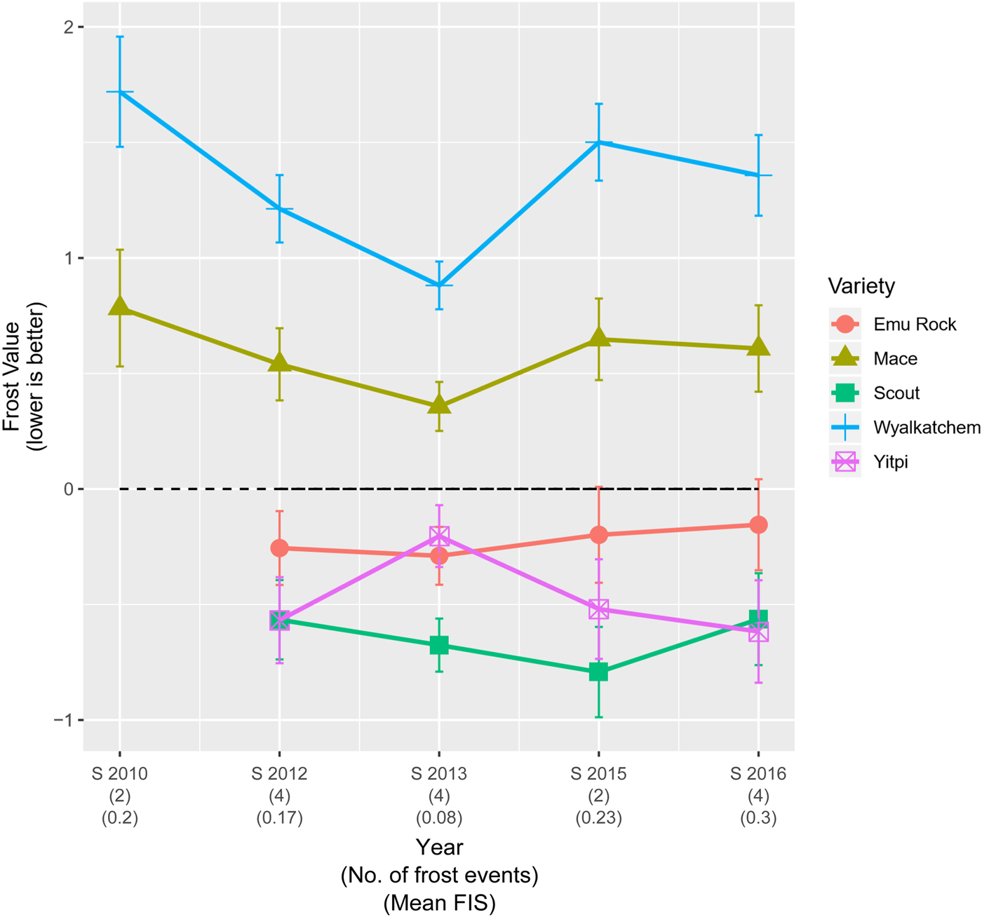
These graphs present the predicted common variety by environment effects (frost values) for the varieties, shown as a shape specific to each variety and the corresponding standard errors of each prediction as error bars. If a variety did not have data in a particular year for that state, its predicted frost value is not presented. The number of FEs and mean FIS for each experiment is also presented to provide the user with more detailed information about the environment that is represented, i.e. frequency and severity of the FEs (mean FIS). The dashed line represents the average frost value at each FEE, where all three varieties in Fig. 7 exhibit lower frost susceptibility in each NSW FEE than the average variety. The positive response of both EGA Gregory and Spitfire to the second factor (Fig. 6) is also evident, where EGA Gregory is less susceptible to frost damage in two of the five environments compared to Suntop. Furthermore, the difference in susceptibility to frost damage between Suntop and Spitfire is also not as large as the difference in OP would suggest because of the response of the latter to the second factor. From Fig. 8, it is clear that Wyalkatchem and to a lesser extent Mace are more highly susceptible to frost damage than the average variety sown in each of the SA FEEs. Furthermore, the relatively large negative response of Yitpi to the second factor is highlighted by the frost value predictions for SA 2012 and SA 2016, where it is as susceptible or less susceptible to frost damage than Scout which had a lower OP (Fig. 3).
Discussion
Screening cereals for frost risk in Australia has become increasingly important over recent years. The enormity of the economic and mental impact of frost on local growers has brought the issue to the forefront as one of the biggest challenges facing the industry. There has been little research undertaken to date as the challenges of not only designing a suitable experiment but also formulation of an appropriate model for the analysis is not to be underestimated. Furthermore, the provision of this information to local growers, breeders and researchers in an informative, valuable and user-friendly format is crucial. This is discussed in detail in the following.
To achieve the key outputs of the Australian National Frost Project (and Screening for Frost Tolerance in Cereals project), the trait of interest (FIS), measurement protocols and derivation of the plot and treatment structures for a single FEE and the MET dataset were fundamental to the statistical approach for analysis. The complexity of these structures and the unbalanced nature of the data necessitated the use of an LMM approach adopted by Smith et al. (Reference Smith, Ganesalingam, Kuchel and Cullis2015) and Gogel et al. (Reference Gogel, Smith and Cullis2018). The LMM included terms that reflected the inherent nature of the randomization of treatments to plots, the longitudinal nature of the data arising from potential repeated measurements over the course of the experiment and features of interest reflected in the measurement protocol such as SOD at tagging.
Since the FEEs are sown across the Australian wheat-belt, it was expected that real and substantial VEI exists in the dataset. This is of importance to the growers, breeders and researchers. The growers would wish to examine the performance of varieties in environments that experience similar conditions to their own farms. The breeders and researchers on the other hand would be interested in exploiting this information across all environments in identifying varieties that are highly adaptive and therefore consistently exhibit low frost risk in all environments to introgress this trait into their own breeding programmes. The VEI in the MET dataset was captured in the LMM by fitting an FA model to Expt:Variety as proposed by Smith et al. (Reference Smith, Ganesalingam, Kuchel and Cullis2015) and subsequently Gogel et al. (Reference Gogel, Smith and Cullis2018), to provide frost value predictions for each variety for every environment in the MET dataset.
The results from the fitted model have allowed dissemination of information at both the regional level for growers and across the growing regions as a whole. The PV-PLUS plots (Smith et al., Reference Smith, Ganesalingam, Kuchel and Cullis2015) provide an excellent interactive summary to the growers of variety performance across years within states or across all states and years if they wish. They can then filter the environments based on those FEEs that are representative of the environmental influences that they also commonly expect for their own farms.
The selection tools more recently developed by Smith and Cullis (Reference Smith and Cullis2018) in the plant breeding context are also useful in this setting. Not only would these summary tools provide information to the growers but would also prove useful to both breeders and researchers. Growers would use these tools as an initial overview to then identify a set of varieties to inspect using PV-PLUS graphs to further understand their behaviour. A breeder would be able to isolate a set of high performing lines (low OP) and determine characteristics of each with the aim of introducing these traits into their breeding programme. They can also investigate those that appear to be at higher risk and make use of the information that distinguishes these from the remaining wheat varieties to understand frost damage within the crop.
There is still further research required in the frost risk of not only cereals but all crops in Australia. It is important that understanding of the physiology of these crops continues to evolve to modify the protocols used in the current FEEs if appropriate. These modifications are then catered for in the statistical approach taken to analyse the resulting dataset. Therefore, the methods outlined in the current paper are subject to change due to this and to reduce the level of unexplained variation in the current modelling approach.
Acknowledgement
We gratefully acknowledge financial support of the Grains Research and Development Corporation of Australia and thank them for use of the data. We acknowledge the work of Simon Diffey in the initial development of the shiny app used to develop the PV-PLUS graphs. We also thank Paul McGowan for his efforts in data collation and auditing. We also gratefully thank the referees for comments and their suggestions that significantly improved the final manuscript. In particular, we are grateful for the suggestion of a logit transformation of the data that lead to the re-analysis of the dataset and further research beyond the scope of this paper.
Financial support
This work was funded by the Grains Research and Development Corporation of Australia.
Conflict of interest
On behalf of all authors, the corresponding author states that there is no conflict of interest.
Ethical standards
Not applicable.