1 Introduction
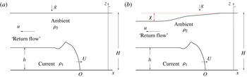
Benjamin’s (Reference Benjamin1968) analysis of the steady-state gravity current is a fundamental and seminal theoretical contribution to the field. The configuration is sketched in figure 1(a): a layer of fluid of density
 $\unicode[STIX]{x1D70C}_{1}$
and height
 $h$
(the ‘current’) propagates with constant speed
 $U$
into another motionless fluid of density
 $\unicode[STIX]{x1D70C}_{2}~({<}\unicode[STIX]{x1D70C}_{1})$
and height
 $H~({>}h)$
(the ‘ambient’). Shear effects on the boundaries of the system are neglected. This renders a reduction to a large domain of flows, with essentially an infinite number of combinations of densities
 $\unicode[STIX]{x1D70C}_{1},\unicode[STIX]{x1D70C}_{2}$
and heights
 $h,H$
, into one compact formula
 $\mathit{Fr}=\mathit{Fr}(a)=U/(g^{\prime }h)^{1/2}$
, valid for
 $a\leqslant a_{max}=1/2$
. (Here,
 $a=h/H$
, and
 $g^{\prime }$
is the reduced gravity; see (2.2).) Admittedly, a careful consideration of this derivation gives rise to various objections concerning the applicability to real gravity currents with large Reynolds number
 $Re=Uh/\unicode[STIX]{x1D708}$
produced by realistic initial conditions and confined by realistic solid boundaries (
 $\unicode[STIX]{x1D708}$
is the typical kinematic viscosity of the fluids). Nevertheless, this is a classical and indispensable result, which still inspires extensions and interpretations (e.g. Shin, Dalziel & Linden Reference Shin, Dalziel and Linden2004; Ungarish Reference Ungarish2006, Reference Ungarish2009, Reference Ungarish2016; White & Helfrich Reference White and Helfrich2008; Borden & Meiburg Reference Borden and Meiburg2013; Milewski & Tabak Reference Milewski and Tabak2015; Konopliv et al.
Reference Konopliv, Llewellyn Smith, McElwaine and Meiburg2016).
A severe restriction of Benjamin’s (Reference Benjamin1968) analysis is the presence of a fixed-height top,
 $z=H$
. It is emphasized in that paper that an insightful simple model is possible ‘if, first, the fluid is given a fixed upper boundary at a finite height above the bottom’ (p. 213). The various published rederivations and extensions, see above, have accepted this constraint. However, gravity currents often appear in open-surface channels. The intriguing practical and theoretical question is whether an open-top counterpart flow, as sketched in figure 1(b), exists, and, if yes, what is the solution. The answer is the topic of this paper.
Qualitatively, the open-surface problem introduces the effect of decrease in the height,
 $\unicode[STIX]{x1D712}$
. In the fixed-top case,
 $\unicode[STIX]{x1D70C}_{2}U^{2}\sim \unicode[STIX]{x0394}\unicode[STIX]{x1D70C}gh$
, where
 $\unicode[STIX]{x0394}\unicode[STIX]{x1D70C}=\unicode[STIX]{x1D70C}_{1}-\unicode[STIX]{x1D70C}_{2}$
. An observer attached to the current notes that the speed of the stream increases from
 $U$
to
 $u_{2}=U/(H-h)$
from front to back, with a corresponding increase of kinetic energy. By opening the top streamline to a constant pressure, that increase of kinetic energy must be balanced (using the Bernoulli equation) by
 $\unicode[STIX]{x1D70C}_{2}g\unicode[STIX]{x1D712}$
, and hence
 $\unicode[STIX]{x1D712}/h\sim \unicode[STIX]{x0394}\unicode[STIX]{x1D70C}/\unicode[STIX]{x1D70C}_{2}$
is expected. On the other hand, this
 $\unicode[STIX]{x1D712}$
contraction of the return flow in the ambient will then hinder propagation and reduce
 $U$
. Quantitatively, we need a clear-cut system of equations for the coupled
 $U,\unicode[STIX]{x1D712}$
variables, subject to the energy-dissipation constraint. Our analysis provides the details of the formulation and demonstrates that the solutions are physically acceptable. We note in passing that the
 $\unicode[STIX]{x1D712}/h\sim \unicode[STIX]{x0394}\unicode[STIX]{x1D70C}/\unicode[STIX]{x1D70C}_{2}$
estimate is well known, and therefore Benjamin’s analysis has been considered, correctly, to be a valid approximation for Boussinesq systems
 $\unicode[STIX]{x0394}\unicode[STIX]{x1D70C}/\unicode[STIX]{x1D70C}_{2}\ll 1$
with open surfaces in numerous laboratory studies, with little or no comment. Our work adds rigour to this estimate. However, practically, the present results are of interest to non-Boussinesq systems.
The idealized gravity current in the laboratory system. (a) Benjamin’s problem with fixed top
 $z=H$
; (b) the new problem with free-surface top open to constant pressure
 $p=0$
.

2 Formulation
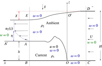
The flow under consideration is sketched in figure 1(b). The analysis is performed in a Cartesian coordinate system attached to the current; see figure 2. The origin
 $O$
is at the leading edge of the current, which is a stagnation point for the ambient fluid. We use a control volume (c.v.) with vertical boundaries
 $\mathit{CD}$
on the upstream and
 $\mathit{BE}$
in the downstream sides. The fluids differ sharply in density,
 $\unicode[STIX]{x1D70C}_{1}>\unicode[STIX]{x1D70C}_{2}$
, and the ‘interface’
 $\mathit{OAA}^{\prime }$
describes this separation. The velocity is
 $\boldsymbol{u}=u\hat{\boldsymbol{x}}+w\hat{\boldsymbol{z}}$
, where
 $u$
and
 $w$
are functions of
 $x$
and
 $z$
. When necessary, we shall add subscripts
 $i=1,2$
for the dense and light fluids receptively. We define the vorticity
 $$\begin{eqnarray}\unicode[STIX]{x1D714}=\hat{\boldsymbol{y}}\boldsymbol{\cdot }\unicode[STIX]{x1D735}\times \boldsymbol{u}=\frac{\unicode[STIX]{x2202}u}{\unicode[STIX]{x2202}z}-\frac{\unicode[STIX]{x2202}w}{\unicode[STIX]{x2202}x}.\end{eqnarray}$$
The current is assumed to be a motionless body of fluid, with
 $u_{1}=w_{1}=\unicode[STIX]{x1D714}_{1}=0$
.
The c.v. attached to the current. Here,
 $\unicode[STIX]{x1D702}$
is, schematically, the thickness of the vortex-wake layer. In § 3, this layer is infinitesimally small, a vortex sheet. The upper boundary is open to the atmosphere,
 $p=0$
. The vorticity
 $\unicode[STIX]{x1D714}=0$
on the
 $\mathit{ABCDE}$
boundary. The sketched values of
 $\unicode[STIX]{x1D714}$
inside the c.v. are expected.

The conditions on the boundary of the c.v. are as follows. The upstream flow has uniform velocity
 $U$
(and hence is irrotational). The downstream flow is parallel – horizontal with
 $u_{2}(z),w_{2}=0$
. On the bottom
 $z=0$
and the top boundaries of the c.v., there is no penetration and free slip, which implies no shear and zero vorticity. At the point
 $A$
(and to the left along
 $z=h$
), there is continuity of pressure and velocity; therefore, in particular,
 $u_{2}(h)=0$
.
We do not specify the flow of the ambient fluid inside the c.v. However, some qualitative features that are physically consistent with the foregoing assumption must be taken into account. In particular, we keep in mind that the
 $\mathit{OA}$
interface (between the current and the ambient) contributes shear and generates vorticity. Due to diffusion and convection,
 $\unicode[STIX]{x1D714}>0$
is expected inside the
 $\mathit{OO}^{\prime }\mathit{EA}$
domain, but
 $\unicode[STIX]{x1D714}=0$
is expected in the
 $\mathit{OCDO}^{\prime }$
part. Although the upstream flow is irrotational and energy conserving, in the c.v., the ambient fluid gains vorticity and dissipates energy (undergoes headloss). As pointed out by Benjamin, these non-ideal-fluid effects, not introduced explicitly, are essential to the gravity current.
Letting
 $$\begin{eqnarray}\left.\begin{array}{@{}c@{}}a=h/H,\quad r=\unicode[STIX]{x1D70C}_{2}/\unicode[STIX]{x1D70C}_{1},\quad \unicode[STIX]{x0394}\unicode[STIX]{x1D70C}=\unicode[STIX]{x1D70C}_{1}-\unicode[STIX]{x1D70C}_{2},\quad g^{\prime }=(1/r-1)g,\\ \quad \mathit{Fr}=U/(g^{\prime }h)^{1/2},\quad \tilde{\unicode[STIX]{x1D712}}=\unicode[STIX]{x1D712}/H,\end{array}\right\}\end{eqnarray}$$
the task is to derive
 $\mathit{Fr}(a,r)$
and
 $\tilde{\unicode[STIX]{x1D712}}(a,r)$
solutions, and determine the range of validity,
 $a\in (0,a_{max}(r)]$
. By
 $a=0$
we mean the limit of a thin, or deep, current
 $h/H\rightarrow 0$
. Benjamin’s flat-top result is denoted by
 $\mathit{Fr}_{b}(a)$
.
The assumed boundary conditions reduce the Navier–Stokes equations in the up- and downstream domains to the hydrostatic pressure
 $\unicode[STIX]{x2202}p/\unicode[STIX]{x2202}z=-\unicode[STIX]{x1D70C}g$
. With the
 $p=0$
condition at the top and continuity at point
 $A$
, we obtain
 $$\begin{eqnarray}\displaystyle & \displaystyle \text{on}~\mathit{CD}\text{:}~p=\unicode[STIX]{x1D70C}_{2}g(H-z)\quad (0\leqslant z\leqslant H); & \displaystyle\end{eqnarray}$$
 $$\begin{eqnarray}\displaystyle & \displaystyle \text{on}~\mathit{BE}\text{:}~p=\left\{\begin{array}{@{}l@{}}\unicode[STIX]{x1D70C}_{2}g(H-\unicode[STIX]{x1D712}-z)\quad (h\leqslant z\leqslant H-\unicode[STIX]{x1D712}),\\ \unicode[STIX]{x1D70C}_{2}g(H-\unicode[STIX]{x1D712}-z)+\unicode[STIX]{x0394}\unicode[STIX]{x1D70C}g(h-z)\quad (0\leqslant z\leqslant h).\end{array}\right. & \displaystyle\end{eqnarray}$$
Consistent with Benjamin’s analysis,
 $O$
is a perfect stagnation point (i.e. there is no headloss; the justification is given in appendix A). We thus write the Bernoulli balance on
 $\mathit{BOC}$
using (2.3) at
 $z=0$
,
 $$\begin{eqnarray}p_{B}=p_{O}={\textstyle \frac{1}{2}}\unicode[STIX]{x1D70C}_{2}U^{2}+\unicode[STIX]{x1D70C}_{2}gH,\end{eqnarray}$$
which yields, using (2.4) at
 $z=0$
to obtain
 $p_{B}$
,
 $$\begin{eqnarray}\unicode[STIX]{x1D712}=\frac{\unicode[STIX]{x0394}\unicode[STIX]{x1D70C}}{\unicode[STIX]{x1D70C}_{2}}h-\frac{1}{2}\frac{U^{2}}{g}.\end{eqnarray}$$
In dimensionless form, using
 $\tilde{\unicode[STIX]{x1D712}}=\unicode[STIX]{x1D712}/H$
and the definition of
 $\mathit{Fr}$
, this is expressed as
 $$\begin{eqnarray}\tilde{\unicode[STIX]{x1D712}}=\left(\frac{1}{\displaystyle r}-1\right)a\left(1-\frac{1}{2}\mathit{Fr}^{2}\right).\end{eqnarray}$$
This is a fundamental relationship in our analysis. It provides an explicit dependence between the unknown quantities
 $\tilde{\unicode[STIX]{x1D712}}$
and
 $\mathit{Fr}$
. As expected, the height reduction of the open surface is significant only for non-Boussinesq non-deep currents. We restrict the investigation to positive
 $\unicode[STIX]{x1D712}$
, i.e. the open surface dips over the current. We note that a negative
 $\unicode[STIX]{x1D712}$
is formally possible, but this is associated with high-speed flows with
 $\mathit{Fr}^{2}>2$
, which are expected to be in the problematic supercritical (with respect to the internal shallow-water waves, or characteristics) regime, as briefly discussed in appendix B. Moreover, the generation of a current with large speed may require an energy source, which is not expected in common circumstances.
The volume balance is
 $$\begin{eqnarray}HU=\int _{h}^{H-\unicode[STIX]{x1D712}}u_{2}(z)\,\text{d}z.\end{eqnarray}$$
Since there are no
 $x$
-shear forces on the c.v. envelope, the global (over the c.v.)
 $x$
-momentum balance is for the flow force
 $\int (\unicode[STIX]{x1D70C}u^{2}+p)\,\text{d}z$
and can be expressed, using (2.3)–(2.4), as
 $$\begin{eqnarray}\displaystyle \displaystyle \int _{h}^{H-\unicode[STIX]{x1D712}}u_{2}^{2}(z)\,\text{d}z-U^{2}H & = & \displaystyle \frac{1}{\displaystyle \unicode[STIX]{x1D70C}_{2}}\left(\int _{CD}p\,\text{d}z-\int _{BE}p\,\text{d}z\right)\nonumber\\ \displaystyle & = & \displaystyle \displaystyle g^{\prime }hH\left[-\frac{1}{2}a+\left(\frac{1}{\displaystyle r}-1\right)^{-1}\frac{\tilde{\unicode[STIX]{x1D712}}}{a}\left(1-\frac{1}{2}\tilde{\unicode[STIX]{x1D712}}\right)\right].\end{eqnarray}$$
We eliminate the
 $\tilde{\unicode[STIX]{x1D712}}/a$
term on the right-hand side by (2.7), and, with some algebra, the momentum equation is reduced to
 $$\begin{eqnarray}\frac{1}{g^{\prime }hH}\int _{h}^{H-\unicode[STIX]{x1D712}}u_{2}^{2}(z)\,\text{d}z-\frac{1}{2}\mathit{Fr}^{2}\left(1+\frac{1}{2}\tilde{\unicode[STIX]{x1D712}}\right)=1-\frac{1}{2}(a+\tilde{\unicode[STIX]{x1D712}}).\end{eqnarray}$$
We consider Bernoulli’s balance on the streamline
 $\mathit{DE}$
, where
 $p=0$
and the speed increases from
 $U$
to
 $u_{E}$
. For generality, we allow headloss
 $\unicode[STIX]{x1D70C}_{2}g^{\prime }\unicode[STIX]{x1D6FF}_{t}$
(the subscript means top), to write
 $u_{E}^{2}/2-g\unicode[STIX]{x1D712}=U^{2}/2-g^{\prime }\unicode[STIX]{x1D6FF}_{t}$
. Combining with (2.6), we obtain
 $$\begin{eqnarray}{\textstyle \frac{1}{2}}u_{E}^{2}=g^{\prime }h-g^{\prime }\unicode[STIX]{x1D6FF}_{t}.\end{eqnarray}$$
We argue that (2.11) expresses the vorticity balance for the c.v. The left-hand side is the integral of
 $u\unicode[STIX]{x1D714}=u(\unicode[STIX]{x2202}u/\unicode[STIX]{x2202}z)$
over the boundary
 $\mathit{BE}$
, i.e. this is the vorticity fluxed out from the c.v. It should be noted that (i) there is zero vorticity convection into the c.v. because
 $\unicode[STIX]{x1D714}=0$
on
 $\mathit{ABCDE}$
and (ii) there is zero vorticity diffusion on
 $\mathit{EABCD}$
because the normal
 $\unicode[STIX]{x2202}\unicode[STIX]{x1D714}/\unicode[STIX]{x2202}n$
vanishes on these boundaries. Consequently, the first term on the right-hand side represents the vorticity production inside the c.v. and the second term on the right-hand side is the vorticity diffusion on the boundary
 $\mathit{DE}$
. Indeed, the headloss on
 $\mathit{DE}$
is a result of shear from inside the c.v., associated with the integral of
 $-\unicode[STIX]{x1D708}(\unicode[STIX]{x2202}\unicode[STIX]{x1D714}/\unicode[STIX]{x2202}\unicode[STIX]{x1D701})$
along the line, where
 $\unicode[STIX]{x1D701}$
is in the normal direction; see appendix A.
This ends the formulation. The solution requires the specification of the profile
 $u_{2}(z)$
.
3 The classical constant-
 $u_{2}$
vortex-sheet model

We postulate that
 $u_{2}(z)=u_{2}=u_{E}$
for
 $z>h$
. This is the exact counterpart of Benjamin’s solution. The transition from
 $u_{2}(h)=0$
to the constant value occurs in an infinitesimally thin layer, i.e. a vortex sheet (in figure 2,
 $\unicode[STIX]{x1D702}\rightarrow 0$
). The continuity equation (2.8) gives
 $u_{2}=U/(1-a-\tilde{\unicode[STIX]{x1D712}})$
, and then the momentum equation (2.10), combined with the definition of
 $\mathit{Fr}$
, is simplified to
 $$\begin{eqnarray}\frac{1}{2}\mathit{Fr}^{2}\left[\frac{1+a+\tilde{\unicode[STIX]{x1D712}}}{1-a-\tilde{\unicode[STIX]{x1D712}}}-\frac{1}{2}\tilde{\unicode[STIX]{x1D712}}\right]=1-\frac{1}{2}(a+\tilde{\unicode[STIX]{x1D712}}).\end{eqnarray}$$
Equation (3.1) must be solved together with (2.7), repeated below for convenience:
 $$\begin{eqnarray}\tilde{\unicode[STIX]{x1D712}}=\left(\frac{1}{\displaystyle r}-1\right)a\left(1-\frac{1}{2}\mathit{Fr}^{2}\right).\end{eqnarray}$$
The elimination of
 $\tilde{\unicode[STIX]{x1D712}}$
between (3.1) and (3.2) yields a cubic equation for
 $\mathit{Fr}^{2}$
, but the coefficients are cumbersome and the analytical solution is not insightful. A numerical iterative solution for
 $\mathit{Fr},\tilde{\unicode[STIX]{x1D712}}$
is straightforward, and in this case the use of the system (3.1)–(3.2) is convenient.
The constant value
 $u_{2}=u_{E}$
implies that on any streamline from
 $\mathit{CD}$
to
 $\mathit{AE}$
, the Bernoulli equation predicts the same headloss,
 $\unicode[STIX]{x1D6FF}(z)=\unicode[STIX]{x1D6FF}_{t}$
. Consequently, the rate of dissipation is given by
 $\dot{{\mathcal{D}}}=\unicode[STIX]{x1D70C}_{2}g^{\prime }UH\unicode[STIX]{x1D6FF}_{t}$
, with
 $\unicode[STIX]{x1D6FF}_{t}$
calculated from (2.11). It is evident that the range of validity of the model is determined by the condition
 $\unicode[STIX]{x1D6FF}_{t}\geqslant 0$
, which can be expressed as
 $$\begin{eqnarray}\frac{\unicode[STIX]{x1D6FF}_{t}}{h}=1-\frac{1}{2}\mathit{Fr}^{2}\frac{1}{\displaystyle (1-a-\tilde{\unicode[STIX]{x1D712}})^{2}}\geqslant 0.\end{eqnarray}$$
The energy-conserving solution corresponds to the equality sign.
This model can recover Benjamin’s solution. To this end, we replace the open-surface condition (3.2) by the flat-top condition
 $\tilde{\unicode[STIX]{x1D712}}=0$
. Then, (3.1) and (3.3) yield Benjamin’s results,
 $\mathit{Fr}_{b}^{2}(a)=(2-a)(1-a)/(1+a)$
and
 $\unicode[STIX]{x1D6FF}_{t}/h=1-\mathit{Fr}_{b}^{2}/(2(1-a)^{2})$
. On the other hand, since for the open-top case
 $\tilde{\unicode[STIX]{x1D712}}=0$
for
 $r\rightarrow 1$
, we conclude that the present results converge to Benjamin’s results in this limit, in particular
 $\mathit{Fr}(a,r=1)=\mathit{Fr}_{b}(a)$
.
Results for the open-surface
 $\unicode[STIX]{x1D712}>0$
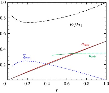
currents are displayed in figures 3–5, in the range of validity. The major conclusion is that the open-surface problem has a physically acceptable solution for a wide range of parameters. Several interesting features appear. First, the range of validity is
 $a\leqslant a_{max}(r)\approx 0.5r$
. Second, for a fixed
 $r$
, the largest
 $\tilde{\unicode[STIX]{x1D712}}$
is attained for the energy-conserving
 $a=a_{max}$
. This
 $\tilde{\unicode[STIX]{x1D712}}_{max}(r)$
is not a monotonic function of
 $r$
, rather like
 $0.45r^{1/4}(1-r)$
. The global (over
 $r$
) maximum is
 $\tilde{\unicode[STIX]{x1D712}}_{max}\approx 0.25$
at
 $r\approx 0.2$
. This has an important implication: it is not possible to produce very large
 $\unicode[STIX]{x1D712}$
by keeping
 $h$
and
 $H$
constant and increasing
 $\unicode[STIX]{x1D70C}_{1}/\unicode[STIX]{x1D70C}_{2}\rightarrow \infty$
(decreasing
 $r\rightarrow 0$
). Third,
 $\mathit{Fr}$
is not much affected by
 $r$
; for most of the range of validity,
 $\mathit{Fr}(a,r)$
is only slightly smaller than
 $\mathit{Fr}_{b}(a)$
. Fourth, the gravity currents are dissipative. As in Benjamin’s solution, for a fixed
 $r$
, the rate of dissipation increases as
 $a$
decreases from
 $a_{max}$
, i.e. the current becomes thinner in a fixed
 $H$
.
The concern with this solution is the
 $z$
-constant headloss,
 $\unicode[STIX]{x1D6FF}(z)=\unicode[STIX]{x1D6FF}_{t}$
. The same difficulty is encountered in Benjamin’s result. The constant
 $\unicode[STIX]{x1D6FF}$
means that shear/vorticity is present over the entire
 $z$
-span of the
 $\mathit{AOO}^{\prime }E$
domain, so that all streamlines that cross the c.v. can be affected and acquire headloss. This feature of the flow is a consequence of the mathematical simplification
 $u_{2}=$
const., but the physical justification is weak. A model that relaxes the need for shear/headloss far away from the internal interface
 $\mathit{OAA}^{\prime }$
is expected to be beneficial, at least as a means of validation of the present results. This is developed in the next section.
4 The velocity transition-layer vortex-wake model
The foregoing analysis demonstrates that a non-constant
 $u_{2}$
is necessary for a non-constant headloss
 $\unicode[STIX]{x1D6FF}(z)$
. Following Benjamin’s idea of a wake-like velocity profile, we argue that a transition velocity layer above
 $z=h$
will concentrate the vorticity and headloss in this domain, and in particular allow for
 $\unicode[STIX]{x1D6FF}_{t}=0$
at the top. We assume the generic profile
 $$\begin{eqnarray}u_{2}(z)=u_{E}\left[1-\unicode[STIX]{x1D719}(z)\right];\quad \unicode[STIX]{x1D719}=1~(z=h),~\unicode[STIX]{x1D719}=0~(z\geqslant h+\unicode[STIX]{x1D702}),\end{eqnarray}$$
where
 $\unicode[STIX]{x1D719}$
is some monotonic decreasing function. The constant
 $\unicode[STIX]{x1D702}$
is the thickness of the vortex wake, assumed to be small compared with the gap
 $\mathit{AE}$
. This is a new variable in our problem, and will be determined by the c.v. balances.
For further use, we introduce
 $$\begin{eqnarray}\left[\unicode[STIX]{x1D6FC}\,\unicode[STIX]{x1D702},\unicode[STIX]{x1D6FD}\,\unicode[STIX]{x1D702},\unicode[STIX]{x1D6FE}\,\unicode[STIX]{x1D702}\right]=\int _{h}^{H-\unicode[STIX]{x1D712}}\left[\unicode[STIX]{x1D719},2\unicode[STIX]{x1D719}-\unicode[STIX]{x1D719}^{2},(1-\unicode[STIX]{x1D719})(2\unicode[STIX]{x1D719}-\unicode[STIX]{x1D719}^{2})\right]\text{d}z,\end{eqnarray}$$
where
 $\unicode[STIX]{x1D6FC},\unicode[STIX]{x1D6FD},\unicode[STIX]{x1D6FE}$
are positive constants of order 1. In our calculations we use, with a slight modification, the exponential
 $\unicode[STIX]{x1D719}=\exp [-(z-h)/\unicode[STIX]{x1D702}]$
, and take the upper boundary of integration in (4.2) at
 $\infty$
because
 $\unicode[STIX]{x1D702}$
is assumed (and later confirmed) to be significantly smaller than the interval
 $\mathit{AE}$
. For this
 $\unicode[STIX]{x1D719}$
, we obtain
 $\unicode[STIX]{x1D6FC},\unicode[STIX]{x1D6FD},\unicode[STIX]{x1D6FE}=1,3/2,5/6$
. (The linear
 $\unicode[STIX]{x1D719}=1-(z-h)/\unicode[STIX]{x1D702}$
, with
 $\unicode[STIX]{x1D6FC},\unicode[STIX]{x1D6FD},\unicode[STIX]{x1D6FE}=1/2,2/3,1/4$
, was also tested and gives very similar results.) We define the dimensionless
 $\tilde{\unicode[STIX]{x1D702}}=\unicode[STIX]{x1D702}/H$
.
Plot of
 $a_{max}$
,
 $\tilde{\unicode[STIX]{x1D712}}_{max}$
and energy-conserving
 $\mathit{Fr}(a_{max},r)$
scaled with
 $\mathit{Fr}_{b}(a_{max})$
versus
 $r$
. The dotted line adjacent to
 $a_{max}$
is
 $0.5r$
. The
 $a_{\mathit{crit}}$
line is the critical flow limitation, explained in appendix B. The same plot results for both models.

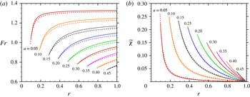
Plots of
 $\mathit{Fr}$
and
 $\tilde{\unicode[STIX]{x1D712}}$
versus
 $r$
for various values of
 $a$
in the range of validity. The solid lines are for the classical model and the dashed lines are for the vortex-wake model.

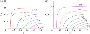
(a) Rate of dissipation
 $\dot{{\mathcal{D}}}/[\unicode[STIX]{x1D70C}_{2}(g^{\prime }h)^{3/2}h]$
versus
 $r$
for various values of
 $a$
. The solid lines are for the classical model and the dashed lines are for the vortex-wake model. (b) The
 $\unicode[STIX]{x1D702}/h$
of the vortex-wake model versus
 $r$
for various values of
 $a$
.

This model is consistent with the physical expectation that the vorticity inside the c.v., and hence headloss, is present only near the interface
 $\mathit{AO}$
, while the flow near and on the
 $\mathit{DE}$
line is irrotational. This gives the condition
 $\unicode[STIX]{x1D6FF}_{t}=0$
, upon which (2.11) yields
 $$\begin{eqnarray}u_{E}=(2g^{\prime }h)^{1/2},\end{eqnarray}$$
and then the continuity equation (2.8), (4.2) and the definition of
 $\mathit{Fr}$
give
 $$\begin{eqnarray}U=(2g^{\prime }h)^{1/2}(1-a-\tilde{\unicode[STIX]{x1D712}}-\unicode[STIX]{x1D6FC}\tilde{\unicode[STIX]{x1D702}}),\quad \mathit{Fr}=\sqrt{2}(1-a-\tilde{\unicode[STIX]{x1D712}}-\unicode[STIX]{x1D6FC}\tilde{\unicode[STIX]{x1D702}}).\end{eqnarray}$$
Substitution into the momentum equation (2.10), and use of (4.2), yields
 $$\begin{eqnarray}2(1-a-\tilde{\unicode[STIX]{x1D712}}-\unicode[STIX]{x1D6FD}\tilde{\unicode[STIX]{x1D702}})-(1-a-\tilde{\unicode[STIX]{x1D712}}-\unicode[STIX]{x1D6FC}\tilde{\unicode[STIX]{x1D702}})^{2}\left(1+{\textstyle \frac{1}{2}}\tilde{\unicode[STIX]{x1D712}}\right)=1-{\textstyle \frac{1}{2}}(a+\tilde{\unicode[STIX]{x1D712}}),\end{eqnarray}$$
and similarly the relationship (2.7) is reduced to
 $$\begin{eqnarray}\tilde{\unicode[STIX]{x1D712}}=\left(\frac{1}{\displaystyle r}-1\right)a(a+\tilde{\unicode[STIX]{x1D712}}+\unicode[STIX]{x1D6FC}\tilde{\unicode[STIX]{x1D702}})(2-a-\tilde{\unicode[STIX]{x1D712}}-\unicode[STIX]{x1D6FC}\tilde{\unicode[STIX]{x1D702}}).\end{eqnarray}$$
We obtain a system of two equations, (4.5)–(4.6), for the variables
 $\tilde{\unicode[STIX]{x1D712}},\tilde{\unicode[STIX]{x1D702}}$
; the solution is obtained numerically. Then,
 $\mathit{Fr}$
follows from (4.4b
).
The range of validity of this model is straightforward: only solutions with
 $\unicode[STIX]{x1D702}\geqslant 0$
are physically acceptable. This is consistent with the energy-dissipation criterion, as follows. Using the Bernoulli equation, we find that the energy loss on a streamline is given by
 $$\begin{eqnarray}g^{\prime }\unicode[STIX]{x1D6FF}(z)={\textstyle \frac{1}{2}}[u_{E}^{2}-u_{2}^{2}(z)]=g^{\prime }h[1-(1-\unicode[STIX]{x1D719})^{2}]\quad (h\leqslant z\leqslant H-\unicode[STIX]{x1D712}).\end{eqnarray}$$
The rate of dissipation, which is the integral of
 $\unicode[STIX]{x1D70C}_{2}u_{2}(z)g^{\prime }\unicode[STIX]{x1D6FF}(z)$
over
 $\mathit{AE}$
, can then be expressed as
 $\dot{{\mathcal{D}}}=\unicode[STIX]{x1D70C}_{2}\sqrt{2}(g^{\prime }h)^{3/2}\unicode[STIX]{x1D6FE}\unicode[STIX]{x1D702}$
, with
 $\unicode[STIX]{x1D6FE}=5/6$
for the present exponential
 $\unicode[STIX]{x1D719}$
(see (4.2)). The energy-conserving solution corresponds to
 $\unicode[STIX]{x1D702}=0$
, and in general
 $\unicode[STIX]{x1D702}\geqslant 0$
yields acceptable dissipation.
A comparison between the predictions of the models (constant
 $u_{2}$
with vortex sheet versus
 $u_{2}(z)$
with vortex wake) was performed. We emphasize that both models share the same range of validity,
 $a\in (0,a_{max}(r)]$
, and coincide at the energy-conserving
 $a_{max}(r)$
(where
 $\unicode[STIX]{x1D6FF}_{t}=\unicode[STIX]{x1D702}=0$
). Figure 3 applies to both models. Figure 4 displays the
 $\mathit{Fr}(a,r)$
and
 $\tilde{\unicode[STIX]{x1D712}}$
predictions of the vortex-wake model (dashed lines). The present
 $\mathit{Fr}$
is slightly smaller, while the present
 $\tilde{\unicode[STIX]{x1D712}}$
is slightly larger, than the counterpart predictions of the classical vortex-sheet model (for fixed
 $r$
, the discrepancies are 0 at
 $a_{max}$
and attain 2 %–3 % for small
 $a$
). The behaviour of
 $\dot{{\mathcal{D}}}$
is qualitatively the same in both models; see figure 5(a). The vortex-wake model is in general less dissipative (the discrepancy attains approximately 20 % for small
 $a$
and
 $r\approx 1$
). Since the dissipation is just a byproduct of the solution for
 $\mathit{Fr},\tilde{\unicode[STIX]{x1D712}}$
, the exact value of
 $\dot{{\mathcal{D}}}$
is of minor importance (given that the order of magnitude and the parametric trend are the same in both models).
The vortex-wake thickness
 $\unicode[STIX]{x1D702}$
, scaled with
 $h$
, is displayed in figure 5(b). The results confirm that this is a physically acceptable non-large variable. The
 $\unicode[STIX]{x1D702}/h$
value is larger for deep currents (small
 $a$
). However, we keep in mind that this layer represents a sub-domain of
 $u_{2}(z)$
in the thick ambient; on the
 $H=h/a$
scale,
 $\unicode[STIX]{x1D702}$
is always small. We conclude that the vortex-wake model is a useful solution, valuable on its own and in particular as a support to the classical model.
5 Concluding remarks
We have presented a comprehensive analysis of the idealized steady-state current of height
 $h$
and density
 $\unicode[STIX]{x1D70C}_{1}$
that propagates into an ambient unperturbed fluid of height
 $H$
and density
 $\unicode[STIX]{x1D70C}_{2}$
with an upper surface open to the atmosphere (open channel), at large
 $\mathit{Re}$
. This is a significant extension of Benjamin’s (Reference Benjamin1968) seminal solution for a fixed-top channel. The current propagates with
 $U$
and causes a depth decrease
 $\unicode[STIX]{x1D712}$
of the top surface.
The dimensionless parameters of the problem are
 $a=h/H$
and
 $r=\unicode[STIX]{x1D70C}_{2}/\unicode[STIX]{x1D70C}_{1}$
. We showed that a control volume analysis determines
 $\tilde{\unicode[STIX]{x1D712}}=\unicode[STIX]{x1D712}/H$
and
 $\mathit{Fr}=U/(g^{\prime }h)^{1/2}$
as functions of
 $a$
and
 $r$
. The balances are for volume and momentum (explicitly), and vorticity (implicitly). The solution is self-contained without any adjustable constants. The results are obtained numerically. The currents are in general dissipative, and thus valid only for
 $a\leqslant a_{max}(r)\approx 0.5r$
. The current with height
 $h=a_{max}H$
is energy conserving. The value of
 $\mathit{Fr}(a,r)$
is typically smaller than that of Benjamin’s
 $\mathit{Fr}_{b}(a)$
, but the reduction is not dramatic, typically a few per cent. For a given
 $r$
, the maximum height depression is attained for the energy-conserving
 $a_{max}$
, and is
 $\tilde{\unicode[STIX]{x1D712}}_{max}\approx 0.45r^{1/4}(1-r)$
. The global maximum, attained at
 $r\approx 0.2$
, is
 $\tilde{\unicode[STIX]{x1D712}}_{max}\approx 0.25$
; this point also corresponds to the global minimum of
 $\mathit{Fr}(a,r)/\mathit{Fr}_{b}(a)$
, which is approximately 0.75.
We have developed two models for the solution of the c.v. balances. The first assumes that the outflow
 $u_{2}$
is
 $z$
-independent, accompanied by a similarly homogeneous headloss. The
 $z=h$
interface is a vortex sheet. This is exactly the counterpart of Benjamin’s solution. The second model assumes that
 $u_{2}(z)$
increases from
 $0$
over a vortex-wake layer of finite thickness
 $\unicode[STIX]{x1D702}$
(say) above
 $z=h$
, and the headloss occurs in this layer only. (The details of the
 $u_{2}(z)$
profile have a minor quantitative influence; here, we used a physically plausible exponential-increase function). The
 $\mathit{Fr},\tilde{\unicode[STIX]{x1D712}}$
results of the two models are in excellent agreement, and this increases the confidence concerning the physical relevance of the global analysis.
The open-surface counterpart to Benjamin’s current has been an open problem for five decades. We hope that this paper will close this gap of knowledge. Admittedly, both the vortex-sheet and the vortex-wake models are strong idealizations. The steady-state flow must be consistent with the initial and boundary conditions, which is usually attainable when
 $U$
is subcritical (or at most critical) with respect to the speed of the characteristic. This, however, turns out to produce only a mild additional restriction
 $a\leqslant a_{\mathit{crit}}$
, discussed in appendix B and displayed in figure 3. In a realistic flow, the interface shear domain spreads (mildly) with
 $\sqrt{x}$
behind the c.v., as already pointed out by Benjamin; moreover, the free-slip bottom can be realized in Navier–Stokes simulations, but in the laboratory and nature some (small but finite) shear is present. Still, the analysis is expected to provide the correct parametric insights, be a fair approximation for a limited period/distance of propagation of currents created by a constant source or lock release, and be useful as a ‘jump condition’ at the nose of more complicated currents. To the best of our knowledge, no data for a reliable comparison with the present theory are available. The available open-channel laboratory studies for the considered problem are for Boussinesq liquids with
 $r\approx 1$
. In this case,
 $\unicode[STIX]{x1D712}/H$
is small, and the difference between the open-surface and fixed-top flows is insignificant. This (near) coincidence is well known, and numerous published Boussinesq laboratory studies with open-top systems rely (correctly) on Benjamin’s fixed-top results with little or no comment. A reliable corroboration of our results needs non-Boussinesq systems with various values of
 $a$
. Laboratory tests, and Navier–Stokes simulations, for such currents with an open surface are difficult tasks. We hope that this study will provide motivation and guidelines for such works in the future.
Acknowledgement
The author thanks an anonymous referee for pointing out the critical flow issue, and Professor A. J. Hogg for helpful discussions.
Appendix A. The stagnation point versus headloss
$\unicode[STIX]{x1D6FF}_{t}$

We consider figure 2. Following Benjamin, in our analysis,
 $O$
is a perfect stagnation point (i.e. there is no headloss on the
 $\mathit{CO}$
streamline), while on the
 $\mathit{DE}$
streamline, headloss
 $\unicode[STIX]{x1D6FF}_{t}>0$
is allowed. Here, we provide a brief justification.
The streamline
 $\mathit{CO}$
has special conditions: constant height
 $z=0$
,
 $w=0$
and
 $\unicode[STIX]{x1D714}=\unicode[STIX]{x2202}u/\unicode[STIX]{x2202}z=0$
. We use the steady-state
 $x$
-component of the Navier–Stokes momentum equation for the ambient fluid with viscosity
 $\unicode[STIX]{x1D707}_{2}$
, and integrate with
 $x$
from
 $C$
to
 $O$
to obtain
 $$\begin{eqnarray}p_{O}-p_{C}=\frac{1}{2}\unicode[STIX]{x1D70C}_{2}(U^{2}-u_{O}^{2})-\left[-\unicode[STIX]{x1D707}_{2}\int _{\mathit{CO}}\frac{\unicode[STIX]{x2202}\unicode[STIX]{x1D714}}{\unicode[STIX]{x2202}z}\,\text{d}x\right];\end{eqnarray}$$
 $u_{O}=0$
by definition. The term in brackets is the headloss (the
 $-$
sign is because energy deficit is defined as positive headloss and dissipation). We argue that this term vanishes due to consideration of vorticity. The upstream flow is irrotational, and there is no mechanism that can produce vorticity to the right of point
 $O$
; therefore,
 $\unicode[STIX]{x1D714}=0$
in the fluid above
 $\mathit{CO}$
. In combination with the free-slip condition
 $\unicode[STIX]{x1D714}=0$
on
 $z=0$
, we conclude that
 $\unicode[STIX]{x2202}\unicode[STIX]{x1D714}/\unicode[STIX]{x2202}z=0$
on
 $\mathit{CO}$
. This validates the
 $p_{O}=(1/2)\unicode[STIX]{x1D70C}_{2}U^{2}$
relationship. It should be noted that we do not rely here on energy arguments; the vorticity consideration indicates that there is no headloss on the
 $\mathit{CO}$
line.
The foregoing vorticity consideration can be applied to the
 $\mathit{DE}$
line using an equation similar to (A 1) for
 $p_{E}-p_{D}$
. The headloss term is an integral of
 $-\unicode[STIX]{x1D707}_{2}\unicode[STIX]{x2202}\unicode[STIX]{x1D714}/\unicode[STIX]{x2202}\unicode[STIX]{x1D701}$
on
 $\mathit{DE}$
, where
 $\unicode[STIX]{x1D701}$
is the normal coordinate. Since vorticity is generated at the
 $\mathit{OA}$
interface,
 $\unicode[STIX]{x1D714}>0$
is present in the ambient to the left of
 $O$
, and hence
 $\unicode[STIX]{x2202}\unicode[STIX]{x1D714}/\unicode[STIX]{x2202}\unicode[STIX]{x1D701}<0$
is possible on
 $\mathit{DE}$
. This can justify the headloss
 $\unicode[STIX]{x1D6FF}_{t}>0$
. We emphasize that, although
 $\mathit{Re}$
is large, we cannot set
 $\unicode[STIX]{x1D707}_{2}=0$
in our models. This would reduce the validity range to the energy-conserving line.
Appendix B. Critical
$U$
and the
$a<a_{\mathit{crit}}$
restriction


The gravity current flow is regulated by characteristics that propagate with velocities
 $c_{\pm }$
(in the laboratory frame) determined by the shallow-water equations. Theory and experiments, see Baines (Reference Baines1995) and Ungarish (Reference Ungarish2011), indicate that a feasible steady-state current cannot move faster than the characteristic
 $c_{+}$
(from the reservoir of dense fluid to the nose); i.e., unless the propagation is subcritical (or at most critical) with
 $c_{+}\geqslant U$
, the flow pattern may be inconsistent with our assumptions. Using the expression for
 $c_{+}$
reported in Ungarish (Reference Ungarish2011), we find that this condition leads to the equation (dimensional)
 $$\begin{eqnarray}g^{\prime }\tilde{H}(1-h/\tilde{H})^{3}\geqslant U^{2},\end{eqnarray}$$
where
 $\tilde{H}=H-\unicode[STIX]{x1D712}$
. Substitution of
 $\tilde{H}=H(1-\tilde{\unicode[STIX]{x1D712}})$
,
 $\tilde{a}=h/\tilde{H}=a/(1-\tilde{\unicode[STIX]{x1D712}})$
and
 $\mathit{Fr}^{2}=U^{2}/(g^{\prime }h)$
yields
 $$\begin{eqnarray}(1-\tilde{a})^{3}\geqslant \mathit{Fr}^{2}\tilde{a}.\end{eqnarray}$$
For the present
 $\mathit{Fr},\tilde{\unicode[STIX]{x1D712}}$
results, equation (B 2) is tantamount to the condition
 $a\leqslant a_{\mathit{crit}}(r)$
. The critical value
 $a_{\mathit{crit}}$
, calculated numerically, is shown in figure 3. For
 $r\approx 1$
, we recover the
 $a_{\mathit{crit}}=0.347$
condition of Benjamin’s analysis. For
 $r>0.68$
,
 $a_{\mathit{crit}}$
is slightly below the energy-dissipation limitation
 $a_{max}$
, and thus critical currents with
 $a=a_{\mathit{crit}}$
are feasible. In this range, the ratio
 $\mathit{Fr}(a,r)/\mathit{Fr}_{b}(a)$
is similar for
 $a_{max}$
and
 $a_{\mathit{crit}}$
. For
 $r<0.68$
, we find that
 $a_{max}<a_{\mathit{crit}}$
, which implies that all energetically valid currents are subcritical. The critical value
 $a_{\mathit{crit}}(r)$
changes insignificantly between the two models. The focus on subcritical
 $U$
introduces a mild additional restriction as concerns the applicability of our analysis.
We note that a current with large
 $\mathit{Fr}$
and negative
 $\unicode[STIX]{x1D712}$
tends to violate (B 2), i.e. is typically supercritical. Moreover,
 $\mathit{Fr}^{2}>2$
is also prone to violate the energy limitation (3.3). These considerations justify why the present analysis has been restricted to
 $\unicode[STIX]{x1D712}>0$
(and hence
 $\mathit{Fr}^{2}<2$
) cases. However, propagation in supercritical conditions and with
 $\unicode[STIX]{x1D712}<0$
(the open surface bulges above the current) is not necessarily precluded. The solution, and conditions of applicability, are expected to be more complex than discussed in this paper, and this topic must be left for future investigation.