1. Introduction
The human ankle is crucial for lower limb movement, balance, and power provision in the human body [Reference Fong, Hong, Chan, Yung and Chan1]. It carries most of the body weight and is essential for activities like walking, standing, and running, making it prone to injury [Reference Czamara, Szuba, Królikowska, Kentel, Krupa, Reichert and Sznajder2]. Traditional ankle rehabilitative exercise is manually conducted by therapists to gradually impulse and restore impaired central nervous systems. Currently, there is a shortage of medical professionals compared to the number of patients, highlighting the need for ankle rehab robots for effective treatment [Reference Zhang, Liu, Liu, Qi, Niu and Guo3].
The series mechanism’s motor cannot be wholly fixed, leading to increased inertial resistance and challenges in fitting the motor in a small ankle space [Reference Meng, Liu, Xu, Meng and Yu4]. In comparison, parallel mechanisms (PMs) offer advantages like smaller error, greater precision, higher loading capacity, simplified control, and stable movement [Reference Meng, Xie, Liu and Takeda5]. Scholars have focused on designing ankle rehabilitative robots based on PMs. For example, Girone et al. [Reference Girone, Burdea, Bouzit, Popescu and Deutsch6] engineered a 6-DOFs foot-ankle rehabilitative robot using the Stewart mechanism, which, despite simulating accurate human ankle movement, has drawbacks like excessive degrees of freedom and high expense. Nurahmi et al. [Reference Nurahmi, Caro and Solichin7] created a 3-DOF ankle rehabilitative robot based on a 3-RPS parallel mechanism, offering a reconstruction strategy and kinematics optimization. Valles et al. [Reference Valles, Cazalilla, Valera, Mata, Page and Diaz-Rodriguez8] designed a cost-effective 3-DOF ankle rehabilitative robot derived from a 3-PRS parallel mechanism, emphasizing kinematics, dynamics, and control methods. This mechanism closely mimics ankle motion, providing a large rotation space at a lower cost. However, it may cause parasitic motion during rotation, leading to discomfort and potential secondary damage for the patient.
Following that, some researchers have simplified the human ankle to a 2-DOFs universal joint (in this paper, expressed in U) joint or a 3-DOFs spherical hinge (expressed in S) and have developed a range of 2-DOFs or 3-DOFs parallel ankle rehabilitative robots (PARRs) [Reference Doroftei, Cazacu and Alaci9, Reference Qu, Li, Yao, Ma and Guo10]. For instance, Dai et al. [Reference Saglia, Dai and Caldwell11–Reference Dai, Zhao and Nester13] created a high-efficiency 3-UPS/U PARR enabling ankle inversion, eversion, dorsiflexion, and plantar flexion movements. Likewise, there are 3-RSS/S [Reference Liu, Gao, Yue, Zhang and Guangda14] and 3-SPS/S [Reference Dai, Zhao and Nester13] PARRs featuring three independent rotatory movements. These mechanisms offer simple structure, excellent kinematical performance, minimal space requirements, and cost-effectiveness. However, these robots may not align perfectly with the human ankle joint center, potentially causing secondary harm, and their range of motion is restricted by the rotation range for the constraint spherical hinge. To address the issue of misalignment between the robot’s rotation center and the human ankle joint center, researchers have proposed various solutions [Reference Shengxian, Zongxing, Jing and Lin15]. Fang et al. [Reference Wang, Fang, Guo and Chen16] introduced a 3-RUS/RRR PM for ankle rehabilitation. Li et al. [Reference Dong, Fan, Li, Zhou, Rong, Kong and Zhou17] developed a 2-UPS/RRR PARR with three rotational DOFs, showing promising kinematical performance for active and passive therapy. Other scholars [Reference Choi, Park, Seo, Lee, Lee and Shim18, Reference Hong, Kim and Yoon19] have created ankle PARRs with remote center of motion (RCM) [Reference Li, Hervé and Huang20] to align the human ankle center with the mechanism’s rotation center. For instance, M. Malosio et al. [Reference Malosio, Negri, Pedrocchi, Vicentini, Caimmi and Tosatti21] designed a complex PARR with RCM founded on the 3-RRR parallel spherical robot (named Agile Eye), achieving effective ankle rehabilitation by positioning the human ankle center near the mechanism’s kinematic center. Hu et al. [Reference Liu, Lu, Ma, Deng, Hu and Zeng22] proposed a human-machine compatible 3-RRCRR PARR based on the human ankle model, which can make the robot motion center coincide with the human motion center. Sun et al. [Reference Ni, Liu, Sun and Sun23] proposed an ankle rehabilitation robot with adjustable motion center of hybrid structure, which has better adaptability.
To customize PARRs for patients with varying physiological structures, researchers have incorporated flexible actuators, joints, and components [Reference Zeng, Liu, Qu, Cong, Hou and Lu24]. Wang et al. [Reference Wang, Wang, Wang, Li, Du, Meng and Zhang25] developed a unique PARR with two degrees of freedom using a rigid-flexible hybrid-driven mechanism based on the 2-SPS/U PM. By integrating flexible transmission parts like springs into the prismatic joints, they enhanced flexibility, safety, and comfort. Jamwal et al. [Reference Jamwal, Hussain, Ghayesh and Rogozina26] introduced a 3-DOF compliance ankle rehabilitative robot with an uncomplicated structure, lightweight, and large reachable space, controlled by pneumatic muscles and ropes. While this robot enhances flexibility and safety in the driving direction through flexible actuators, it remains rigid in the constraint space, limiting error compensation.
Grasping the biomechanical structure of human ankles is essential for designing ankle rehabilitative robots. The human ankle joint comprises the tibiotalar joint and subtalar joint, with non-converging axes, creating a spatial non-uniplanar relationship. However, existing studies often misrepresent the ankle joint as an S or U joint with intersecting rotation axes, leading to discrepancies between the rehabilitative robot’s motion and the actual human ankle movement. This mismatch can result in uncoordinated human-robot motion, non-degree-of-freedom forces on the body, potential secondary damage, and compromised rehabilitative outcomes and comfort. Moreover, existing robots may not accommodate the variations in patients’ physiological structures, as the left and right ankle axes typically incline in opposite directions. Consequently, most ankle rehabilitative robots are unable to address the rehabilitation needs of both feet effectively.
Thus, this paper merges the morphological and anatomic model of the anthropo-ankle to introduce an innovative PARR featuring three rotations and a single translation (3R1T). The mechanism features dual VMC points and a pair of rotation planes, allowing uninterrupted rotation devoid of any parasitic movement. The VMC points coordinates align with the center of both the tibiotalar and subtalar joints, with adjustable distance to cater to different patients’ ankle heights. The robot’s initial attitude can be adjusted to suit variations in patients’ joint axis angles. It selects the appropriate rotation axis to match different patients’ joint angles, ensuring compatibility between human and machine movements, suitable rehabilitation for various patients, convenient wearing, and heightened safety.
To summarize, the key contributions are as follows: establishing a reflective link between the human ankle and rehabilitative mechanism based on motion properties and anatomical models, and proposing a novel equivalence model for the ankle joint to assist in designing ankle rehabilitative robots. Secondly, a novel parallel mechanism with 3R1T DOF is introduced. This mechanism exhibits unique motion characteristics, featuring two virtual center points enabling fixed-point rotation around them. It is suitable for ankle rehabilitation applications. Thirdly, as per the kinematical properties of the mechanism as a series branch chain and applying the DH method, it is possible to establish the inverse kinematics model of the rehabilitative mechanism. Subsequently, global design indices are determined based on local performance indices, taking into account the transmissibility and constrainability of mechanism motion/force to optimize the dimensions of the rehabilitative mechanism. Finally, utilizing the OpenSim biomechanical tool, a human musculoskeletal model merges with a rehabilitative robot to create a human-machine rehabilitative simulation framework, accompanied by the creation of an evaluation index to gauge the impact of rehabilitation.
The structure of the paper is outlined thus: In Section 2, utilizing the morphological structure and movement properties of the human ankle joint, the series equivalence model of the anthropo-ankle is established. According to the series equivalence model, the configuration design of a PARR is performed. Section 3 describes the mechanism’s kinematic characteristic as a sequence of branched chains, leading to the development of an inverse kinematic model for the mechanism. Section 4 considers the prototype’s dimensions and interference collision, analyzing the rehabilitative mechanisms’ kinematic efficiency and workspace through motion/force transmission and constraint metrics. In Section 5, considering constraint performance and transmission performance, the dimension synthesis of the mechanism is executed. Section 6 details the construction of an interactive human-robot rehabilitation simulating model designed to confirm and assess the mechanism’s rehabilitation impact. The conclusion is Section 7.
2. Analysis of the rehabilitative mechanism’s mobility configuration and configuration
2.1. Establishment of human ankle equivalence model
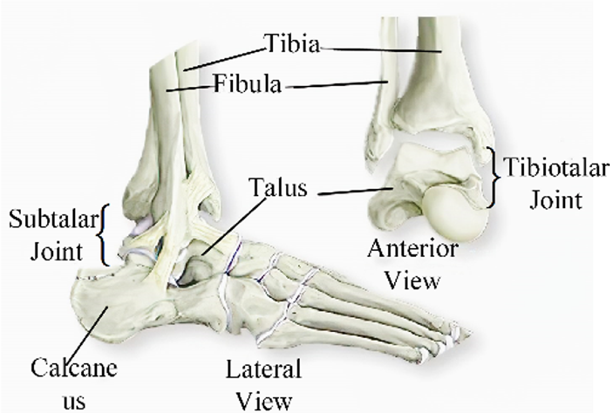
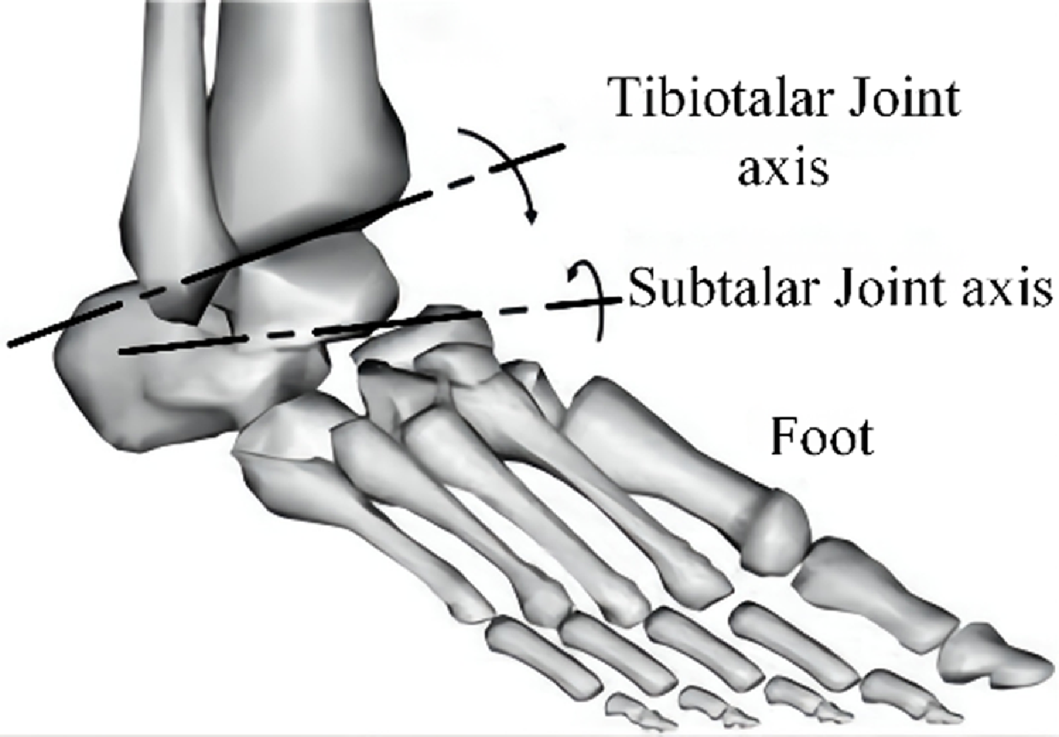
Grasping the morphological structure of human ankles is essential for designing ankle rehabilitative robots. The human ankle is categorized into the narrowed-meaning ankle joint (tibiotalar joint) and the widened meaning ankle joint (tibiotalar joint, talus, and subtalar joint) [Reference Da Silva, Marques and Da Silva27]. Ankle recovery primarily targets the widened-meaning ankle joint, which is complex due to its multiple parts in a confined space: four bones, muscles, and ligaments (see Fig. 1). The tibiotalar joint connects the fibula, tibia, and talus, while the subtalar joint links the calcaneus and talus. The human ankle is a composite structure comprising the subtalar and tibiotalar joints (Fig. 2).
Morphological dissection of the ankle [Reference Alvarez-Perez, Garcia-Murillo and Cervantes-Sánchez28].

Diagram showing the axis of ankle [Reference Saglia, Tsagarakis, Dai and Caldwell29].

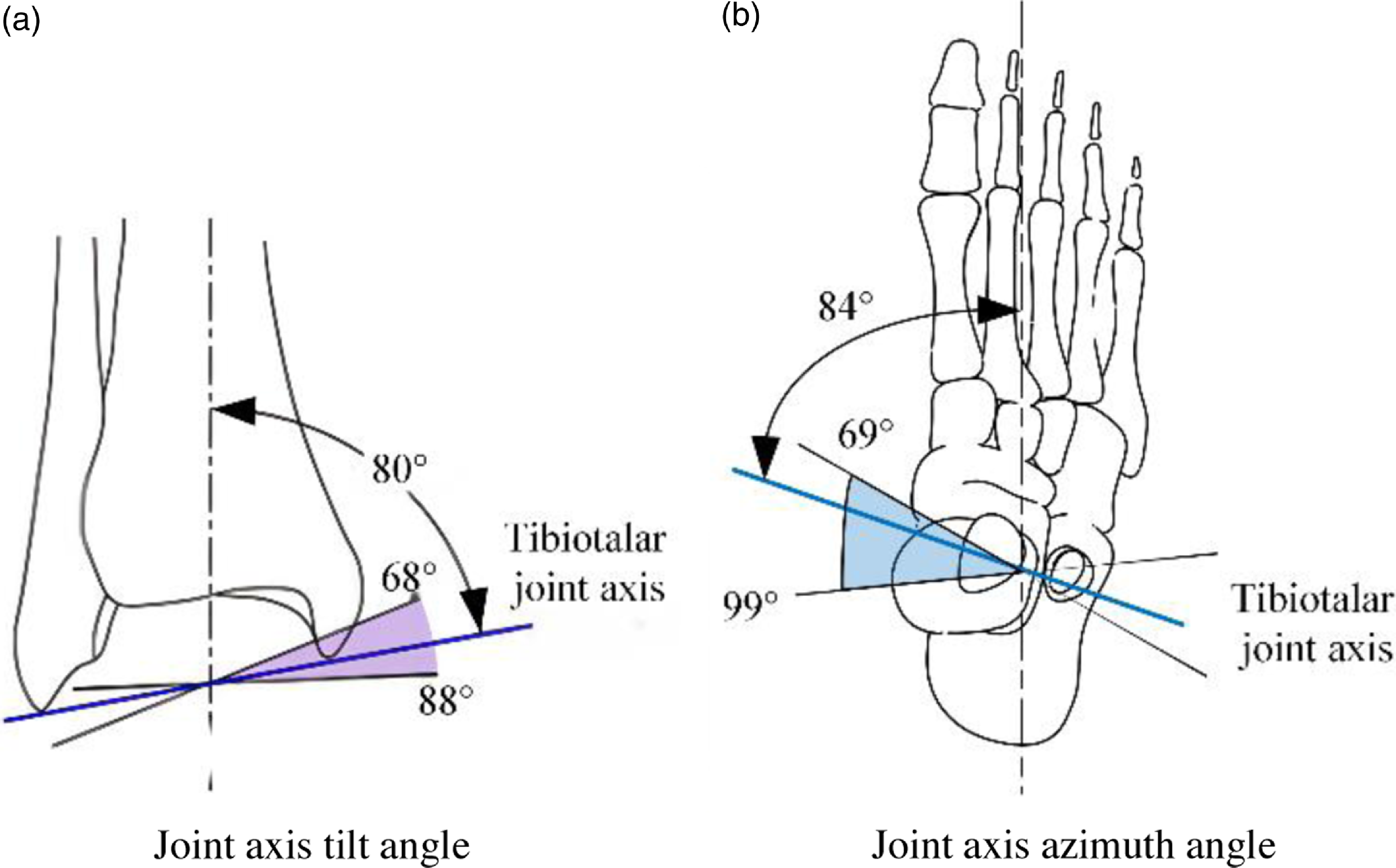
The tibiotalar joint’s axis is defined by the line connecting the forefront of the extramalleolus tip to the mid-point of the internal malleolus tip. Due to the extramalleolus extending further back than the internal malleolus, the tibiotalar joint’s axis joint is tilted vertically and horizontally. It is typically angled at 10° to the cross section and 6° to the coronal section [Reference Weerasingha, Pragnathilaka, Withanage, Ranaweera and Gopura30]. The specific angles can vary among individuals, with the vertical axis angle ranging from 68° to 88° and the sagittal plane angle from 69° to 99° [Reference Stiehl31, Reference Beals32]. Refer to Fig. 3 for illustration.
The tibiotalar joint’s axis [Reference Haskell and Mann33].

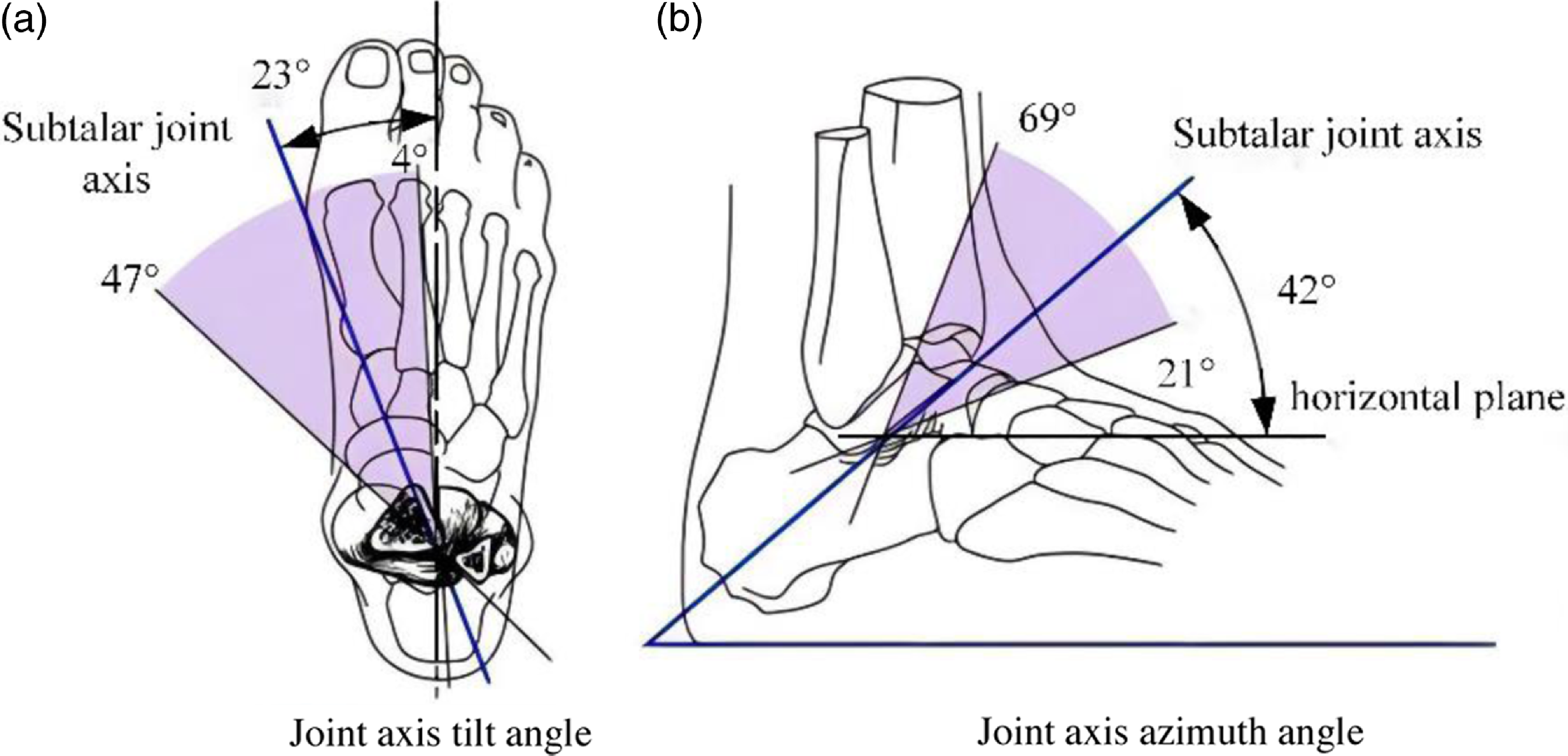
Typically, the subtalar joint’s rotation axis tilts upwards at 42° and inwards at 23°, aligning with the foot’s vertical axis, showing individual variability. The subtalar joint’s tilt angle ranges from 21° to 69°, and the azimuth angle ranges from 4° to 47° [Reference Beals32], as depicted in Fig. 4. The shadow region in the figure represents the range of tilt and azimuth angles, with the blue line indicating the average value.
The subtalar joint’s rotation axis [Reference Jastifer and Gustafson34].

To summarize, the human ankle includes the tibiotalar and subtalar joints, with non-intersecting axes, creating a spatial multiplanar relationship. If a rehabilitative robot does not align with the accurate anatomic structure of the human ankle, it can hinder rehabilitation effectiveness and potentially cause secondary damage. Moreover, due to variations among patients, the axes of these joints differ, making it challenging for most rehabilitative robots to cater to individual rehabilitation requirements.
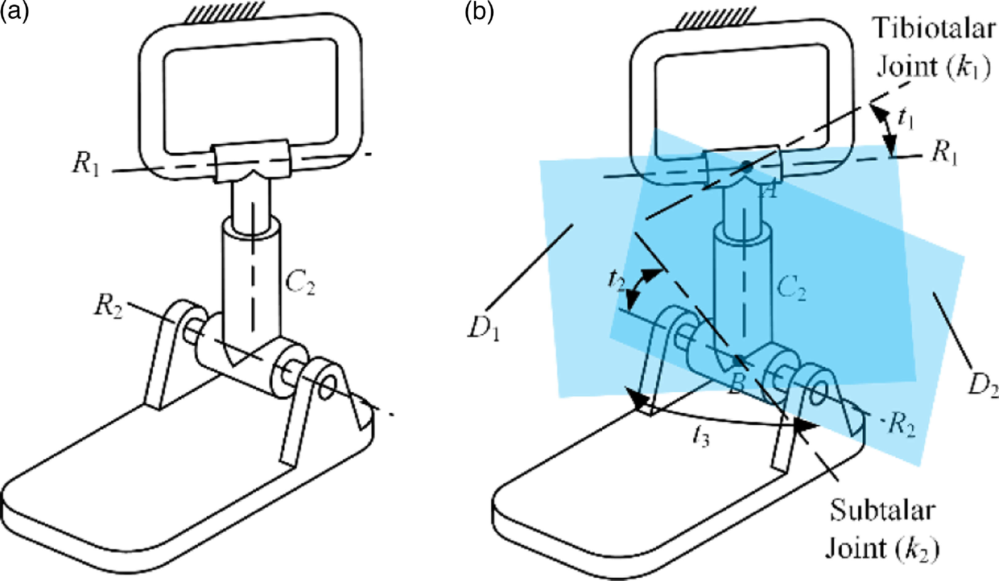
The morphological architecture of the human ankle is influenced predominantly by four factors: the tilt angle of the tibiotalar joint axis (t 1), the tilt angle of the subtalar joint’s axis (t 2), the azimuth angle (t 3) between the tibiotalar joint axis and the subtalar joint axis, and the distance (d) between the tibiotalar joint and the center point of the subtalar joint. Additionally, the human ankle can be likened to a serial R represents a rotating joint, C represents a cylindrical joint (RCR) limb sequence, as depicted in Fig. 5.
The mechanism diagram of the serial RCR ankle model.

The Fig. 5 illustrates that the RCR serial limb has three rotating and one sliding DOF, with rotary centers A and B, and rotary planes D 1 and D 2. Point A is where R 1 and C 2 axes intersect, while point B is the intersection of C 2 and R 2 axes. Rotary planes D 1 and D 2 are formed by the joint axes of R 1/C 2 and R 2/C 2, respectively. The mechanism can rotate continuously around axis k 1 at point A on rotary plane D 1, similar to the tibiotalar joint axis. It can also rotate around axis k 2 at point B on rotary plane D 2, akin to the subtalar joint axis. By using the translational DOF of joint C 2, the distance d between A and B can be modified to suit different ankle heights. The rotational DOF of joint C 2 allows for adjusting the angle t 3 between rotary planes D 1 and D 2 to align with variations in the subtalar and tibiotalar joint axes among different patients.
2.2. Configuration design of parallel rehabilitative mechanism utilizing the RCR model
2.2.1 Motion characteristics analysis of the ankle RCR equivalence model
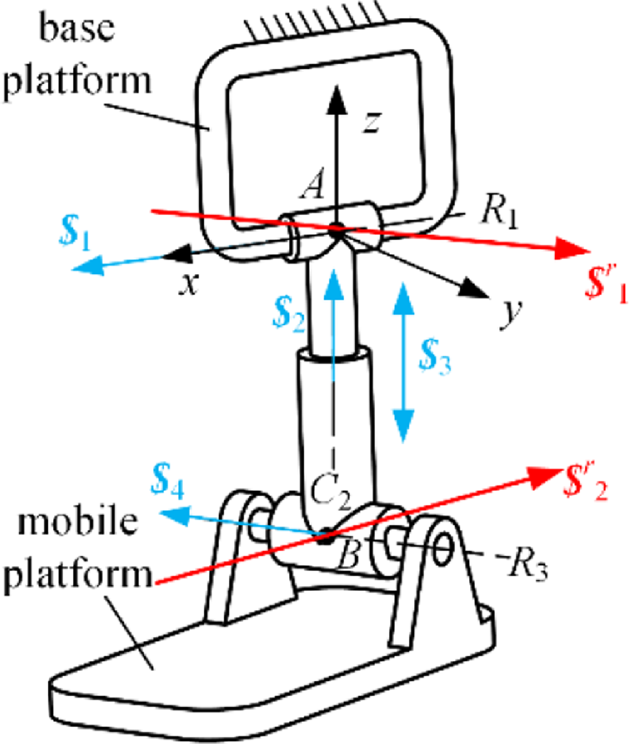
The serial RCR branch features the specific boundary condition: R 1⊥C 2; R 3⊥C 2; R 1 and C 2 meet at point A, with point A being immobile in relation to the ground. Similarly, the crossing point of R 3 and C 2 is at point B, and this point B remains immobile in relation to the moving platform. Construct the branch auxiliary coordinate framework as shown in Fig. 6.
The mechanism diagram of the RCR equivalence model of ankle joint.

The guidelines for establishing the coordinate framework are outlined as follows: the original point is located at fixed pivot point A, aligning the x-axis with the R 1 axis, aligning the z-axis with the central axis of cylindrical joint C 2, and defining the y-axis using the fleming’s right-hand rule. The kinematic screw arrangement for every single branch joint is as follows:
 \begin{equation}\begin{array}{l} \boldsymbol{\$ }_{1}=\left(\begin{array}{l@{\quad}l@{\quad}l@{\quad}l@{\quad}l@{\quad}l} 1 & 0 & 0 & 0 & 0 & 0 \end{array}\right)^{\mathrm{T}}\\ \boldsymbol{\$ }_{2}=\left(\begin{array}{l@{\quad}l@{\quad}l@{\quad}l@{\quad}l@{\quad}l} 0 & 0 & 1 & 0 & 0 & 0 \end{array}\right)^{\mathrm{T}}\\ \boldsymbol{\$ }_{3}=\left(\begin{array}{l@{\quad}l@{\quad}l@{\quad}l@{\quad}l@{\quad}l} 0 & 0 & 0 & 0 & 0 & 1 \end{array}\right)^{\mathrm{T}}\\ \boldsymbol{\$ }_{4}=\left(\begin{array}{l@{\quad}l@{\quad}l@{\quad}l@{\quad}l@{\quad}l} a & b & 0 & c & e & 0 \end{array}\right)^{\mathrm{T}}. \end{array} \end{equation}
The parameters a, b, c, and e are associated with the position and orientation of the motion joint. The constraint screw for this branch can be identified:
 \begin{equation}\begin{array}{l} \boldsymbol{\$ }_{1}^{r}=\left(\begin{array}{l@{\quad}l@{\quad}l@{\quad}l@{\quad}l@{\quad}l} a & b & 0 & 0 & 0 & 0 \end{array}\right)^{\mathrm{T}}\\ \boldsymbol{\$ }_{2}^{r}=\left(\begin{array}{l@{\quad}l@{\quad}l@{\quad}l@{\quad}l@{\quad}l} 1 & 0 & 0 & 0 & d & 0 \end{array}\right)^{\mathrm{T}} \end{array} \end{equation}
Evidently, the RCR branch comprises two vectors of constraint lines:
 $\boldsymbol{\$ }_{1}^{r}$
and
 $\boldsymbol{\$ }_{2}^{r}$
. The vector
 $\boldsymbol{\$ }_{1}^{r}$
traverses point A, aligning with the revolute joint’s R 3 axis, while vector
 $\boldsymbol{\$ }_{2}^{r}$
crosses point B, running parallel to the revolute joint’s R 1 axis, as illustrated in Fig. 6. The pair of limiting factors restrict two translational degrees of freedom in the RCR branch. The mobile platform possesses the capability to shift along the connection path of points A and B and can rotate continuously with AB line as the axis. Furthermore, it has the capability to continuously revolve around any axis in plane composed of the R 3 axis and point A, or any axes in plane composed of the R 1 axes and point B.
2.2.2 Configuration design of the parallel rehabilitative mechanism
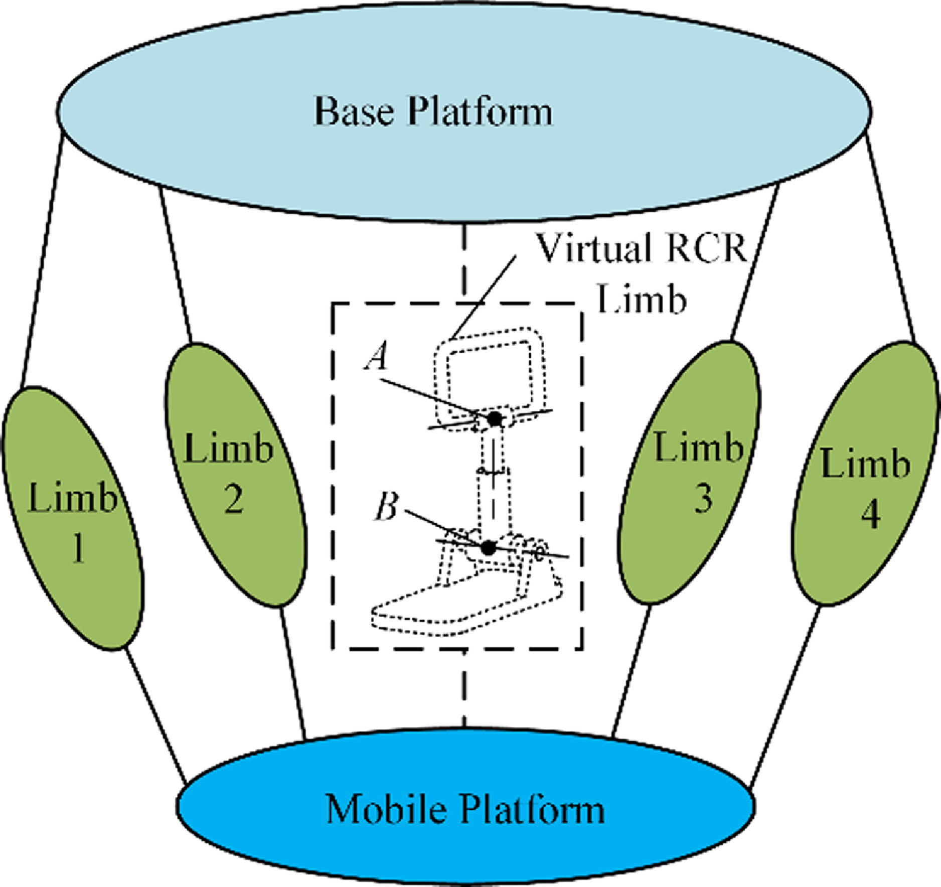
The mechanism utilizes two virtual rotary centers: a fixed center located at A and another center at moving point B, with point B keeping its position comparatively stable on the moving platform. The mobile platform is capable of moving along the line that links points A and B and can continuously rotate about this line. This system offers four independent motion parameters, comprising three rotational motions and one linear movement. Two non-coplanar screws restrict the platform’s translation. One screw consistently passes through the fixed center at A, while the other always traverses the moving center at B. Figure 7 exhibits the schematic representation of the equivalence RCR parallel mechanism.
The design diagram of the equivalence RCR parallel mechanism.

The design schematic of the constraint branch of the parallel mechanism.

When the assembly consists of m branches, the movable platform’s constraint screw system emerges as the most extensive linearly independent set formed by integrating the constraint wrench screw of individual limb. The mobile platform’s constraint wrench screw can be articulated as:
 \begin{equation}\boldsymbol{\$ }^{r}=\overset{m}{\underset{1}\cup }\boldsymbol{\$ }_{j}^{r},\,j=1,\ldots, m \end{equation}
 $\boldsymbol{\$ }^{r}$
indicates the system of constraint screw for the movable platform, while
 $\boldsymbol{\$ }_{j}^{r}$
indicates the system of constraint wrench screw for the j-th limb. The system of constraint wrench screws for the RCR model is described by Eq. (2), from which the twist screw of the fundamental constraint system can be determined. Utilizing point A as the reference point, and applying the concept of reciprocal screws, the basic twist screw of
 $\boldsymbol{\$ }_{1}^{r}$
is:
 \begin{equation}\begin{array}{l} \boldsymbol{\$ }_{m1}=\left(\begin{array}{l@{\quad}l@{\quad}l@{\quad}l@{\quad}l@{\quad}l} 1 & 0 & 0 & 0 & 0 & 0 \end{array}\right)^{\mathrm{T}}\\ \boldsymbol{\$ }_{m2}=\left(\begin{array}{l@{\quad}l@{\quad}l@{\quad}l@{\quad}l@{\quad}l} 0 & 1 & 0 & 0 & 0 & 0 \end{array}\right)^{\mathrm{T}}\\ \boldsymbol{\$ }_{m3}=\left(\begin{array}{l@{\quad}l@{\quad}l@{\quad}l@{\quad}l@{\quad}l} 0 & 0 & 1 & 0 & 0 & 0 \end{array}\right)^{\mathrm{T}}\\ \begin{array}{l} \boldsymbol{\$ }_{m4}=\left(\begin{array}{l@{\quad}l@{\quad}l@{\quad}l@{\quad}l@{\quad}l} 0 & 0 & 0 & 0 & 1 & 0 \end{array}\right)^{\mathrm{T}}\\ \boldsymbol{\$ }_{m5}=\left(\begin{array}{l@{\quad}l@{\quad}l@{\quad}l@{\quad}l@{\quad}l} 0 & 0 & 0 & 0 & 0 & 1 \end{array}\right)^{\mathrm{T}} \end{array} \end{array} \end{equation}
The linear combination of the basic twist screw system is as follows:
 \begin{equation}\begin{array}{l} \begin{array}{l} \boldsymbol{\$ }_{1}=\left(\begin{array}{l@{\quad}l@{\quad}l@{\quad}l@{\quad}l@{\quad}l} 1 & 0 & 0 & 0 & 0 & 0 \end{array}\right)^{\mathrm{T}}\\ \boldsymbol{\$ }_{2}=\left(\begin{array}{l@{\quad}l@{\quad}l@{\quad}l@{\quad}l@{\quad}l} 0 & 1 & 0 & 0 & 0 & 0 \end{array}\right)^{\mathrm{T}}\\ \boldsymbol{\$ }_{3}=\left(\begin{array}{l@{\quad}l@{\quad}l@{\quad}l@{\quad}l@{\quad}l} 0 & 0 & 1 & 0 & 0 & 0 \end{array}\right)^{\mathrm{T}}\\ \boldsymbol{\$ }_{4}=\left(\begin{array}{l@{\quad}l@{\quad}l@{\quad}l@{\quad}l@{\quad}l} 0 & 0 & 0 & 0 & 0 & 1 \end{array}\right)^{\mathrm{T}} \end{array}\\ \boldsymbol{\$ }_{5}=\left(\begin{array}{l@{\quad}l@{\quad}l@{\quad}l@{\quad}l@{\quad}l} 1 & 0 & 0 & 0 & a & 0 \end{array}\right)^{\mathrm{T}} \end{array} \end{equation}
In Eq. (5),
 $ \$ $
1,
 $ \$ $
2, and
 $ \$ $
3 function as a spherical hinge.
 $ \$ $
4 serves as a prismatic joint, and
 $ \$ $
5 represents a revolute joint. The equivalence series branch of the constraint screw
 $ \$ $
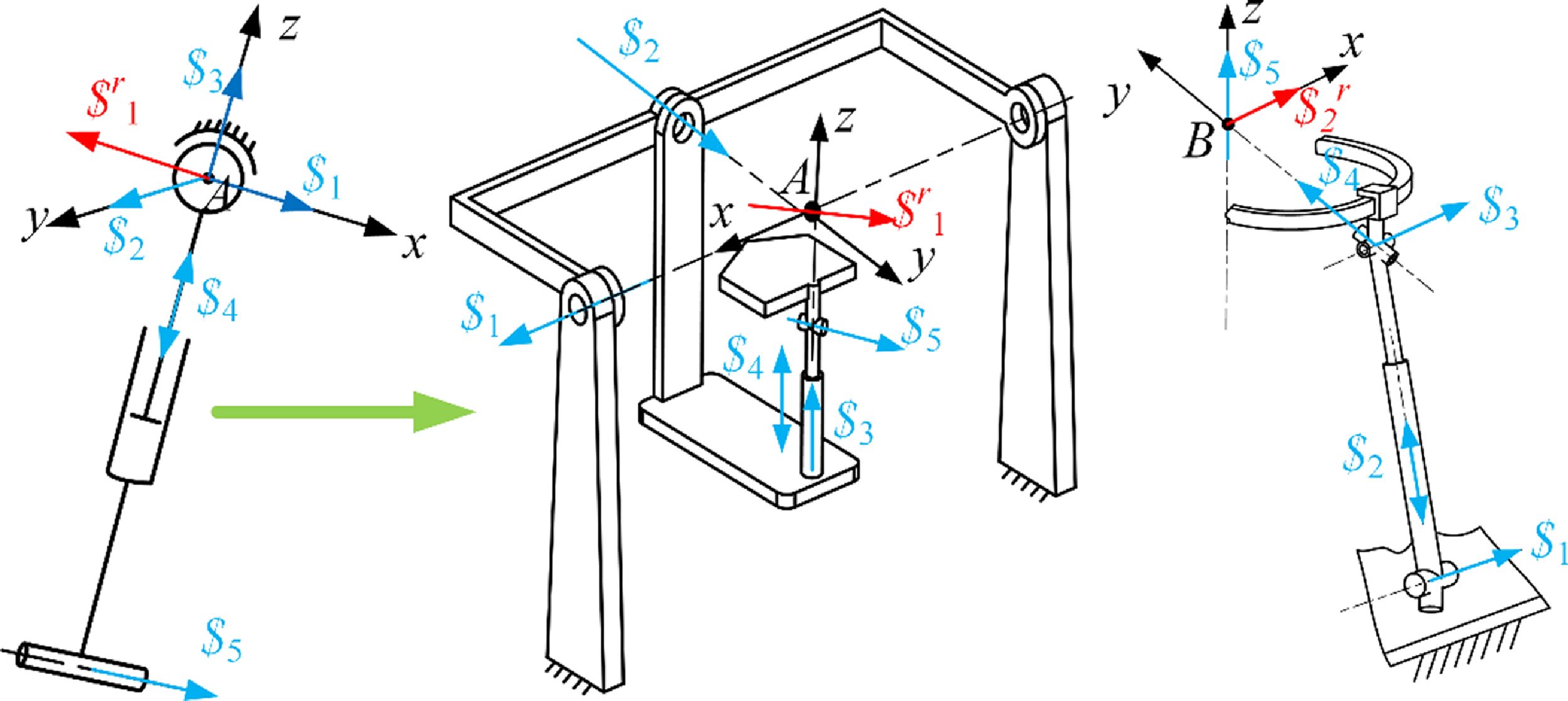
1 forms an SPR branch, as depicted in Fig. 8(a), but the rotation center is the physical center A of the spherical hinge. For the structural topology of the SPR branch, the spherical joint can be divided into three rotational joints intersecting at one point, converting the SPR branch to the RRRPR or R represents a rotating joint, P represents a moving joint, C represents a cylindrical joint (RRCR) branch, as displayed in Fig. 8(b). Similarly, taking point B as the origin, the motion screw system of the constraint screw
 $ \$ $
2 is linearly combined to obtain a new motion screw system.
 \begin{equation}\begin{array}{l} \begin{array}{l} \boldsymbol{\$ }_{1}=\left(\begin{array}{l@{\quad}l@{\quad}l@{\quad}l@{\quad}l@{\quad}l} 1 & 0 & 0 & 0 & m_{1} & n_{1} \end{array}\right)^{\mathrm{T}}\\ \boldsymbol{\$ }_{2}=\left(\begin{array}{l@{\quad}l@{\quad}l@{\quad}l@{\quad}l@{\quad}l} 0 & 0 & 0 & 0 & m_{2} & n_{2} \end{array}\right)^{\mathrm{T}}\\ \boldsymbol{\$ }_{3}=\left(\begin{array}{l@{\quad}l@{\quad}l@{\quad}l@{\quad}l@{\quad}l} 1 & 0 & 0 & 0 & m_{3} & n_{3} \end{array}\right)^{\mathrm{T}}\\ \boldsymbol{\$ }_{4}=\left(\begin{array}{l@{\quad}l@{\quad}l@{\quad}l@{\quad}l@{\quad}l} 0 & 1 & 0 & 0 & 0 & 0 \end{array}\right)^{\mathrm{T}} \end{array}\\ \boldsymbol{\$ }_{5}=\left(\begin{array}{l@{\quad}l@{\quad}l@{\quad}l@{\quad}l@{\quad}l} 0 & 0 & 1 & 0 & 0 & 0 \end{array}\right)^{\mathrm{T}} \end{array} \end{equation}
Setting the rotary center point B as the origin,
 $ \$ $
5 denotes a revolute joint that is in line with the z-axle and traverses origin B;
 $ \$ $
4 is a revolute joint situated in the yz plane, traverses origin B, and converges with
 $ \$ $
5 at the same point;
 $ \$ $
3, another revolute joint, is oriented along the x-axle yet doesn’t traverse origin B;
 $ \$ $
2 is a prismatic joint oriented on the yz plane;
 $ \$ $
1, a revolute joint, also aligned with the x-axis, runs parallel to
 $ \$ $
3 without coinciding with it and similarly avoids crossing the origin B. Thus, the twist system described by Eq. (6) can be likened to an R represents a rotating joint, P represents a moving joint, and U represents a universal joint (RPUR) branch, as depicted in Fig. 8(c). The branch adheres to the constraints imposed by the constraint wrench
 $ \$ $
2 and features a VMC at point B. Even though point B is moving, it remains relatively stationary with respect to the mobile platform.
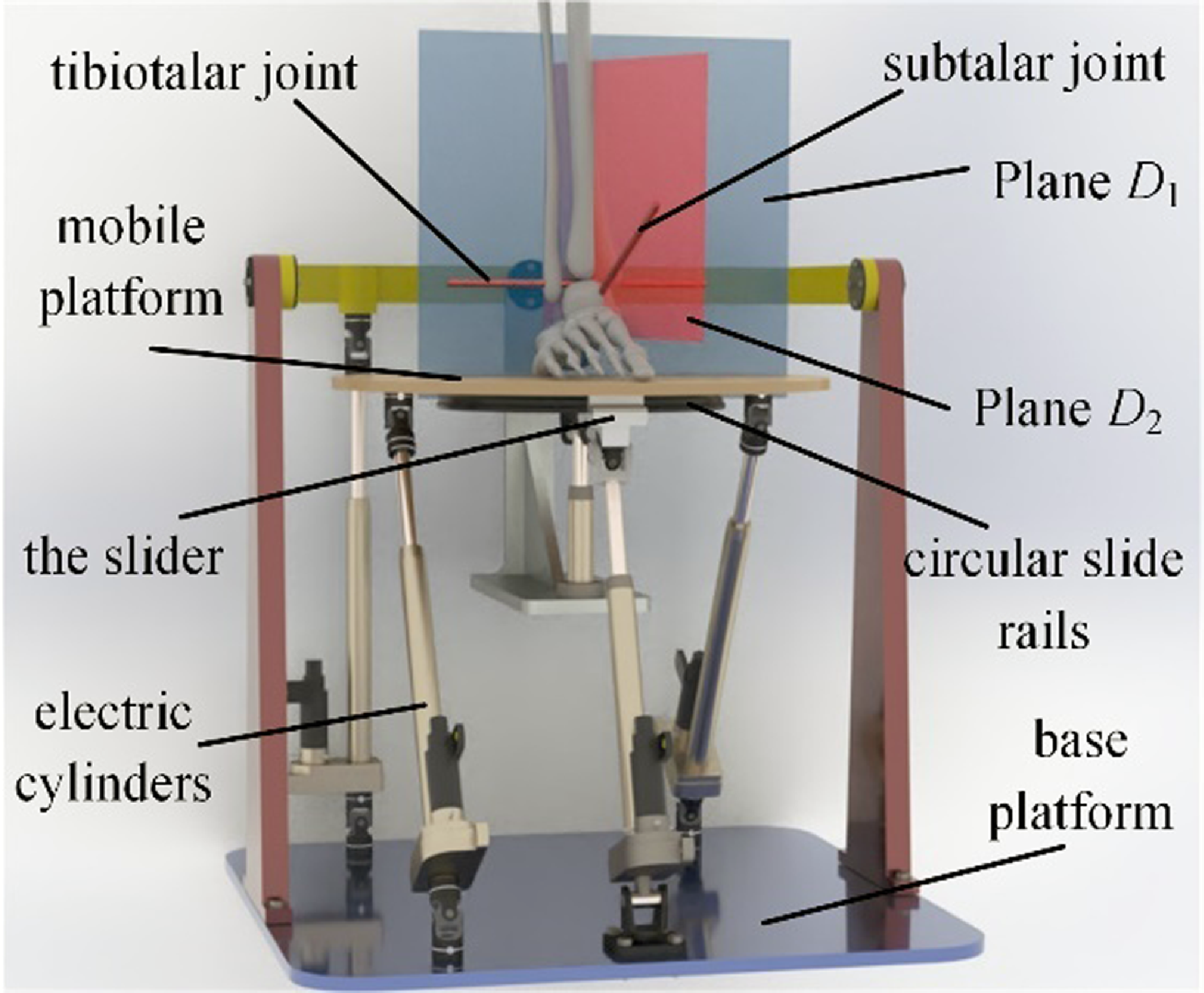
In conclusion, on the basis of the twist and wrench screw systems of the serial RCR ankle joint structure, we designed double types of constraint limbs for the parallel rehabilitative mechanism: one RRCR branch and one RPUR branch. These branches include a stationary virtual rotary center A and a moving virtual rotary center B, separately. By incorporating three unconstrained U represents a universal joint, P represents a moving joint, and S represents spherical joint (UPS) branches as actuation units, an innovative 4-DOFs parallel ankle rehabilitative robot is created. As illustrated in Fig. 9, the robot consists of a mobile platform, a circular sliding track, four electrical actuators, and a base platform. The movement of the mobile platform is controlled by the extension and retraction of the electric actuators, enabling pitch, roll, yaw, and vertical adjustments. The schematic of the parallel rehabilitative mechanism is provided in Fig. 10.
The CAD diagram of the rehabilitative robot.

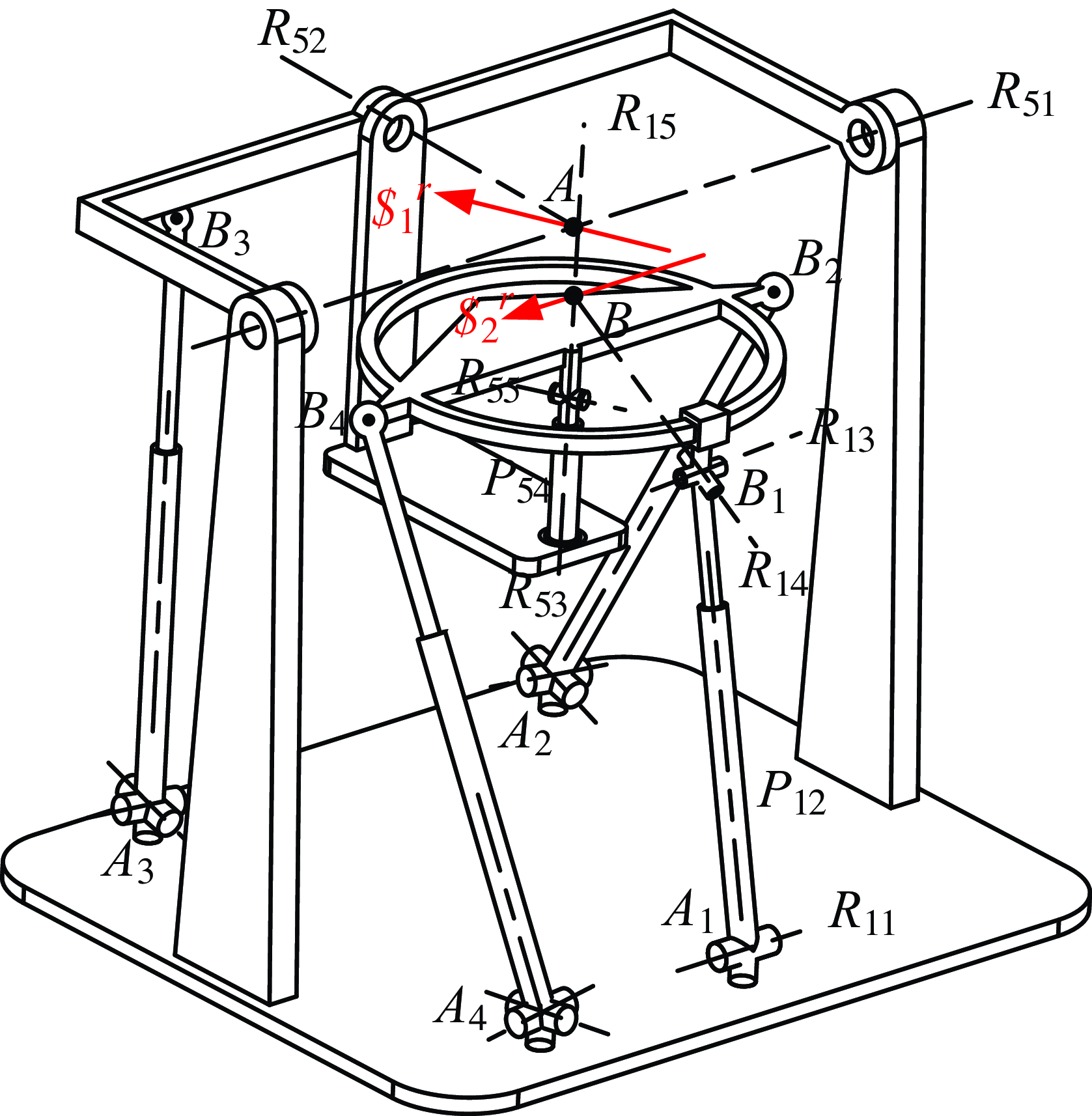
The structure of RRCR/RPUR/3-UPS parallel mechanisms.

The RRCR/RPUR/3-UPS mechanism parameters.

As depicted in Fig. 10, the rehabilitative robot comprises an immobile frame A 1A 2A 3A 4, a moving platform B 1B 2B 3B 4, one RPUR branch, one RRCR passive constraint branch, and three isologous UPS branches. The RPUR limb connects to the mobile platform via the circular sliding track, acting as a revolute joint. The rotary axis R15 of the circular sliding track on the moving platform is fixed and changes with platform movement. Initially, R 15 and R 53 axes are coaxial. The passive constraint branch RRCR is powered by UPS branch A 3B 3.
Every single universal joint is formed by two reciprocally orthogonal revolute joints. The RPUR/RRCR/3-UPS mechanism is depicted in Fig. 10, where R ij denotes the j-th rotary joint in the i-th limb of the rehabilitative robot, and P ij indicates the prismatic joint in the i-th limb of the rehabilitative robot. The mechanism possesses the subsequent boundary condition: R 11⊥P 12; R 11∥R 13; R 51⊥R 52; R 51, R 52, and R 53 intersect at fixed point A; R 14 and R 15 intersect at B point, point B is static compared to the movable platform. The constraint wrench
 $ \$ $
2 through point A aligns with the axis direction of revolute joint R 55. The constraint wrench
 $ \$ $
1 of the RPUR limb traverses point B and is aligned with the axle of the revolute joint R 11. The constraint wrenches of the two limbs are misaligned and traverse VMC A and VMC B separately, as illustrated in Fig. 10.
The two constraint wrenches restrict the two linear movements of the parallel mechanism. Consequently, the moving platform is capable of translating along the AB centerline and possesses three rotary DOFs. This design permits continuous rotation along the AB axis and fixed-point rotation at points A and B.
3. Inverse kinematics modeling of rehabilitative mechanism
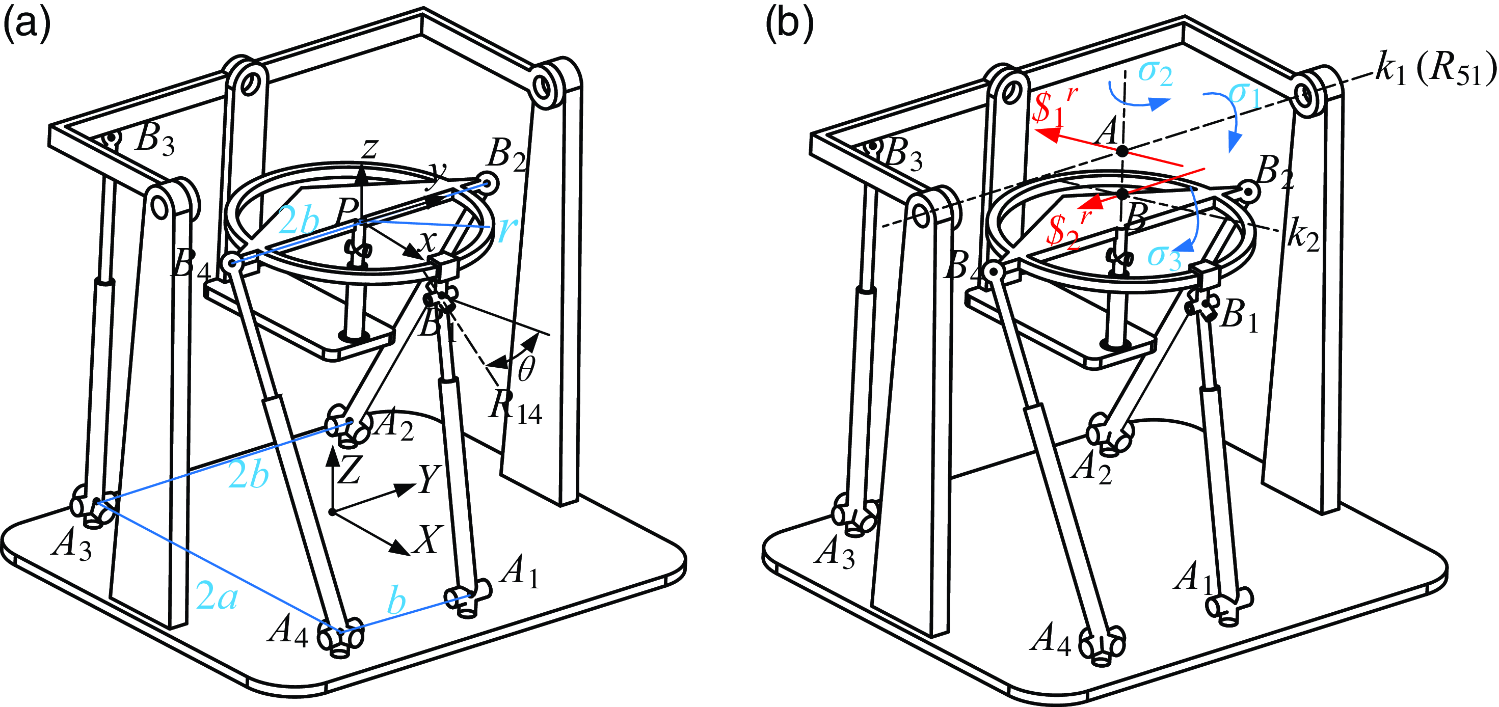
The coordinate framework, as depicted in Fig. 11, is established with the origin O at the center of the fixed platform A 1A 2A 3A 4. The Y-axis is aligned with the revolute joint R 11, and the Z-axis is perpendicular to the base platform. The X-axis follows the right-hand rule. Similarly, the mobile coordinate framework P-xyz is centered at P, the slide rail’s center. The parameters are defined in the following way: A 1A 2 length as 2a, A 2A 3 length as 2b, B 2B 4 length as 2b, A 1A 4 length as b, mobile platform slide rail radius as r, and the tilt angle of the axis of the revolute joint R 14 as θ 2.
In the global coordinate framework O-XYZ, the coordinates of points A and B are represented as:
 \begin{equation}\left\{\begin{array}{l} \boldsymbol{A}=\left[0,0,h_{1}\right]^{\mathrm{T}}\\ \boldsymbol{B}={}^{O}{\boldsymbol{R}}{_{P}^{}}\cdot {}^{P}{\boldsymbol{B}}{}+\boldsymbol{P} \end{array}\right. \end{equation}
In Eq. (7),
 ${}^{O}{\boldsymbol{R}}{_{P}^{}}$
is the rotation matrix of the mobile platform,
 $\boldsymbol{B}^{P}=[0,0,h_{2}]^{\mathrm{T}}, h_{2}=r\cdot \tan (\theta ), \boldsymbol{P}=[x,y,z]^{\mathrm{T}}$
, h 1 is the length of AB, the length of BP is h 2, BP is the position vector of point B in the mobile coordinate framework P-xyz, P is the position vector of the mobile platform in the global coordinate framework O-XYZ.
The orientation of the end effector is decided by several factors: the length d 1 of the line segment between points A and B, and the rotations
 $\sigma _{1}, \sigma _{2}$
, and
 $\sigma _{3}$
around the k1 axis, the AB line segment, and the k 2 axis, respectively. The k 1 axis runs through point A and aligns with the constraint wrench
 $\boldsymbol{\$ }_{1}^{r}$
in the Y-axis direction. Similarly, the k 2 axis traverses point B and aligns with the constraint force vector
 $\boldsymbol{\$ }_{2}^{r}$
. Initially, the angle between planes D 1 and D 2 is
 $\pi /2-\sigma _{0}$
. Given that the human body generally tilts 23° inward at the subtalar joint,
 $\sigma _{0}$
is also set to 23°.
To encapsulate, the kinematic behavior of the mobile platform is analogous to that of a 4-DOFs RCR or RRPR serial manipulator, executing rotations along the k 1 axis, translations along the line connecting points A and B, rotations around this A-B axis, and additional rotations around the k 2 axis. Consequently, the representation of the homogeneous transformation is as depicted below:
 \begin{equation}\begin{array}{l} {}^{A}{\boldsymbol{T}}{_{P}^{}}=\boldsymbol{R}_{y}\left(\sigma _{1}\right)\boldsymbol{R}_{z}\left(\sigma _{0}+\sigma _{2}\right)\boldsymbol{t}_{z}\left(-d_{1}\right)\boldsymbol{R}_{x}\left(\sigma _{3}\right)\boldsymbol{t}_{z}\left(-d_{2}\right)\boldsymbol{R}_{z}\left(-\sigma _{0}\right)\\ =\left[\begin{array}{l@{\quad}l@{\quad}l@{\quad}l} r_{11} & r_{12} & r_{13} & x_{a}\\ r_{21} & r_{22} & r_{23} & y_{a}\\ r_{31} & r_{32} & r_{33} & z_{a}\\ 0 & 0 & 0 & 1 \end{array}\right]=\left[\begin{array}{l@{\quad}l} {}^{O}{\boldsymbol{R}}{_{P}^{}} & {}^{A}{\boldsymbol{P}}{}\\ 0 & 1 \end{array}\right] \end{array} \end{equation}
The positions of point P and the rotational matrix
 ${}^{O}{\boldsymbol{R}}{_{P}^{}}$
for the moving platform are derivable from Eq. (8), where
 $\boldsymbol{P}=\boldsymbol{A}+{}^{A}{\boldsymbol{P}}{}$
. As points B 2 and B 4 are mounted steadily on the platform, their respective positions can be determined using the subsequent expressions:
 \begin{equation}\boldsymbol{B}_{i}={}^{O}{\boldsymbol{R}}{_{P}^{}}\cdot {}^{P}{\boldsymbol{B}}{_{i}^{}}+\boldsymbol{P}\left(i=2,4\right) \end{equation}
Given that point B 1 consistently resides within the XZ plane and moves in relation to the movable platform, the positional coordinates for point B 1 can be represented by the variable
 $[B_{1x},0,B_{1z}]$
. Considering the fixed distance between point B 1 and points P and B, the following limitations apply:
 \begin{equation}\left\{\begin{array}{l} |\boldsymbol{P}-\boldsymbol{B}_{1}|=r\\ |\boldsymbol{B}-\boldsymbol{B}_{1}|=\sqrt{r^{2}+h_{2}^{2}} \end{array}\right. \end{equation}
It can be seen from Fig. 11 that the driving branch A 3B 3 is not directly linked to the mobile platform, but is linked to the RRCR passive constraint branch. Therefore, point B 3 is always on the XZ plane. The coordinates of point B 3 depend on the rotation angle
 $\sigma _{1}$
of the mobile platform around the k 1 axis or R 51 axis:
 \begin{equation}\boldsymbol{B}_{3}=\boldsymbol{R}_{y}\left(\sigma _{1}\right)\cdot {}^{A}{\boldsymbol{B}}{_{3}^{}}+\boldsymbol{A}=\boldsymbol{R}_{y}\left(\sigma _{1}\right)\cdot \left[-a,-b,d_{3}\right]+\boldsymbol{A} \end{equation}
In Eq. (11), d 3 is the coordinate of AB 3 on the Z-axis. The coordinates of point A i on the base platform are as follows:
 \begin{equation}\left\{\begin{array}{c} \boldsymbol{A}_{1}=\left[-a\mathrm{,0,0}\right]^{\mathrm{T}}\\ \boldsymbol{A}_{2}=\left[-a,b,\mathrm{0}\right]^{\mathrm{T}}\\ \boldsymbol{A}_{3}=\left[-a,-b,\mathrm{0}\right]^{\mathrm{T}}\\ \boldsymbol{A}_{4}=\left[a,-b,\mathrm{0}\right]^{\mathrm{T}} \end{array}\right. \end{equation}
By utilizing Eqs. (9), (10), (11), and (12), the positions of points B i and A i within the overall coordinate framework can be determined individually. Consequently, the dimensions of every branch’s prismatic joint are ascertained.
 \begin{equation}L_{i}=\left| \boldsymbol{B}_{i}-\boldsymbol{A}_{i}\right| \end{equation}
4. Kinematic performance and workspace analysis of the mechanism
4.1. Wrench screw and twist screw of the rehabilitative mechanism
Upon securing the branch’s input twist screw (ITS), an additional constraint screw, designated as
 $\boldsymbol{\$ }_{Ti}$
, is introduced. Here,
 $\boldsymbol{\$ }_{Ti}$
represents the branch’s transmission wrench screw (TWS). The product of the TWS in relation to the remaining twist screws is null.
 $\boldsymbol{\$ }_{i}^{r}$
acts as the branch’s constraint wrench screw, while
 $\boldsymbol{\$ }_{Oi}$
serves as the mobile platform’s output twist screw.
 $\boldsymbol{\$ }_{Ri}$
is identified as the branch’s restrictive twist screw, and
 $\bigtriangleup \boldsymbol{\$ }_{Oi}$
is the platform’s restrictive twist screw. Certain interconnections exist among these components as outlined below.
 \begin{equation}\left\{\begin{array}{l@{\quad}l} \boldsymbol{\$ }_{Ti}\circ \boldsymbol{\$ }_{Oj}=0 & \left(i=1,2,3,4;\ i \neq j\right)\\[3pt]\boldsymbol{\$ }_{j}^{r}\circ \boldsymbol{\$ }_{Oi}=0 & \left(i=1,2,3,4;\ j=1,2\right)\\[3pt]\boldsymbol{\$ }_{j}^{r}\circ \bigtriangleup \boldsymbol{\$ }_{Oi}=0& \left(j=1,2;\ j \neq i\right)\\[3pt]\boldsymbol{\$ }_{Ti}\circ \bigtriangleup \boldsymbol{\$ }_{Oj}=0& \left(i=1,2,3,4;\ j=1,2\right) \end{array}\right. \end{equation}
The indices for motion/force transmission within a mechanism are split into two distinct categories: the index for input transmission, denoted as input transmission index (ITI) [Reference Meng, Xie, Liu and Takeda5], and the index for output transmission, referred to as output transmission index (OTI) [Reference Meng, Xie, Liu and Takeda35]. Similarly, the indices for motion/force constraints in a mechanism are bifurcated into an index for input constraints, known as ICI, and an index for output constraints [Reference Liu, Chen and Nahon36, Reference Hu, Shi, Xie, Hu and Ye37].
 \begin{equation}\left\{\begin{array}{l} \lambda _{Ii}=\frac{\left| \boldsymbol{\$ }_{Ti}\circ \boldsymbol{\$ }_{Ii}\right| }{\max \left(\left| \boldsymbol{\$ }_{Ti}\circ \boldsymbol{\$ }_{Ii}\right| \right)}\\[3pt] \lambda _{Oi}=\frac{\left| \boldsymbol{\$ }_{Ti}\circ \boldsymbol{\$ }_{Oi}\right| }{\max \left(\left| \boldsymbol{\$ }_{Ti}\circ \boldsymbol{\$ }_{Oi}\right| \right)}\\ k_{Ii}=\frac{\left| \boldsymbol{\$ }_{i}^{r}\circ \boldsymbol{\$ }_{Ri}\right| }{\max \left(\left| \boldsymbol{\$ }_{i}^{r}\circ \boldsymbol{\$ }_{Ri}\right| \right)}\\[3pt] k_{Oi}=\frac{\left| \boldsymbol{\$ }_{i}^{r}\circ \bigtriangleup \boldsymbol{\$ }_{Oi}\right| }{\max \left(\left| \boldsymbol{\$ }_{i}^{r}\circ \bigtriangleup \boldsymbol{\$ }_{Oi}\right| \right)} \end{array}\right. \end{equation}
Within Eq. (15), the variable
 $\lambda _{Ii}$
signifies the inputting transmission indicator for the i-th branch;
 $\lambda _{Oi}$
represents the outputting transmission index for that same branch;
 $k_{Ii}$
denotes the inputting constraint indicator for the same branch;
 $k_{Oi}$
stands for the outputting constraint indicator for that branch,
 $\boldsymbol{\$ }_{Ii}$
is the input twist screw for the i-th branch.
4.2. Transmission performance analysis
The transmission efficiency ratio represents the force multiplier between the branch inputting twist screw
 $\boldsymbol{\$ }_{Ii}$
and the branch’s TWS
 $\boldsymbol{\$ }_{Ti}$
, as well as the platform’s outputting twist screw
 $\boldsymbol{\$ }_{Oi}$
. The values for both the inputting and outputting efficiency ratios can be derived from Eq. (15). Let’s delineate the local transmission index (LTI) as indicated below:
 \begin{equation}\lambda =\min \left(\lambda _{I\mathrm{i}},\lambda _{oi}\right) \end{equation}
The LTI index is dimensionless and has nothing to do with the selection of the coordinate framework, and the size is between 0 and 1. The higher the value of LTI, the better the motion/force transmission performance of the mechanism under this attitude.
In order to illustrate the relationship between the configuration parameters and the mechanism’s transmission efficiency, specific dimensions of the rehabilitative PM are provided for a sample examination. As depicted in Fig. 11: a = 180 mm, b = 150 mm, and the radius for the sliding track of the end effector is denoted as r, which is 120 mm. The distance between the axes of the subtalar joint and the tibiotalar joint is roughly 30 mm [Reference Dul and Johnson38]. Let d 1 = 30 mm, λ 1 be the rotation angle around the tibiotalar joint axis, and λ 2 be the rotation angle around the subtalar joint axis k 2. The tibiotalar joint axis is considered the horizontal axis k 1, so λ 1 = σ 1. Given that the subtalar joint is inclined inward at an angle of σ 0 degrees and upward by σ 01 degrees (typically σ 0 = 23, σ 01 = 42), the following relationships exist:
 \begin{equation}\sigma _{2}=\lambda _{2}\cdot \sin \left(\sigma _{01}\right),\sigma _{3}=\cos \left(\sigma _{01}\right) \end{equation}
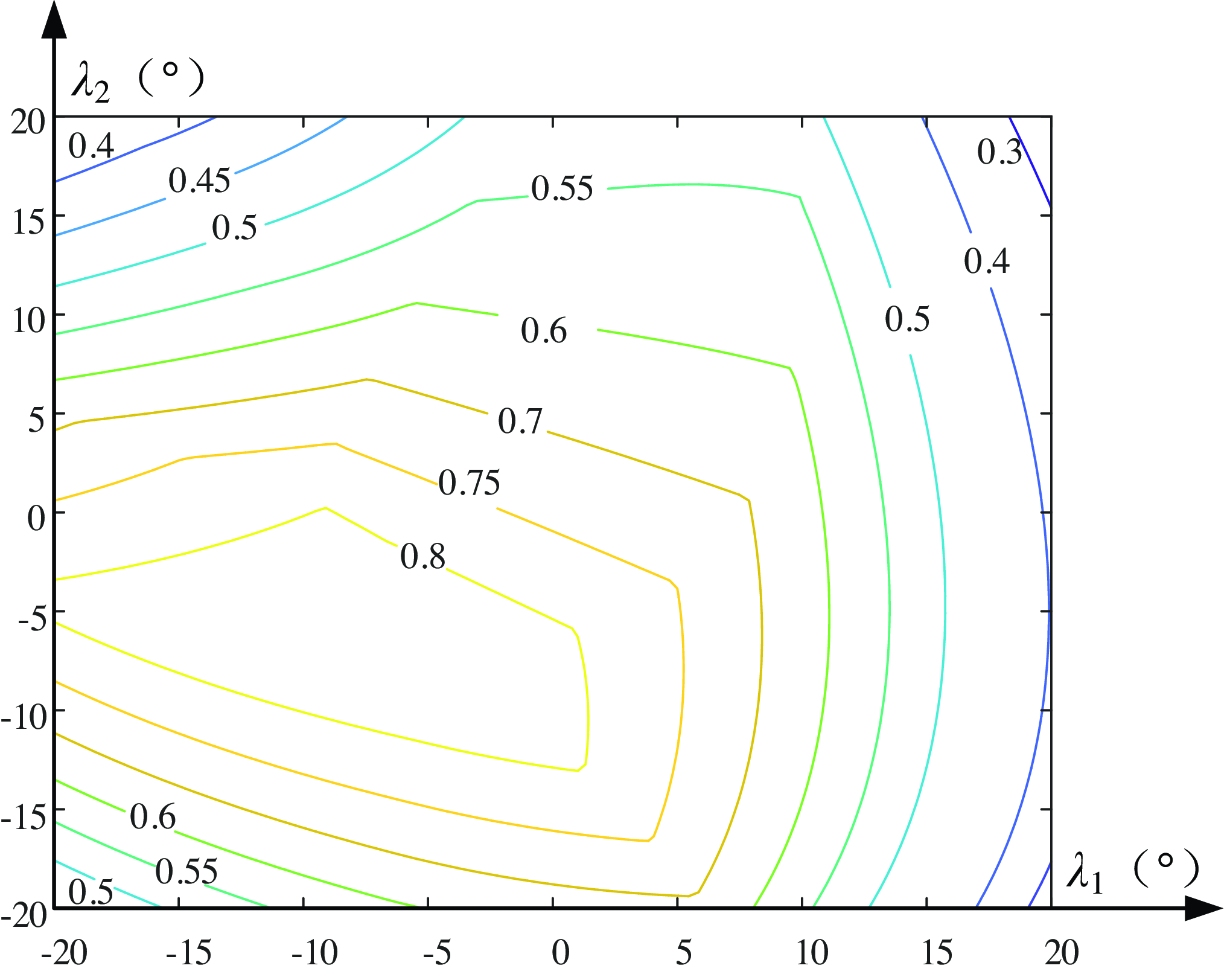
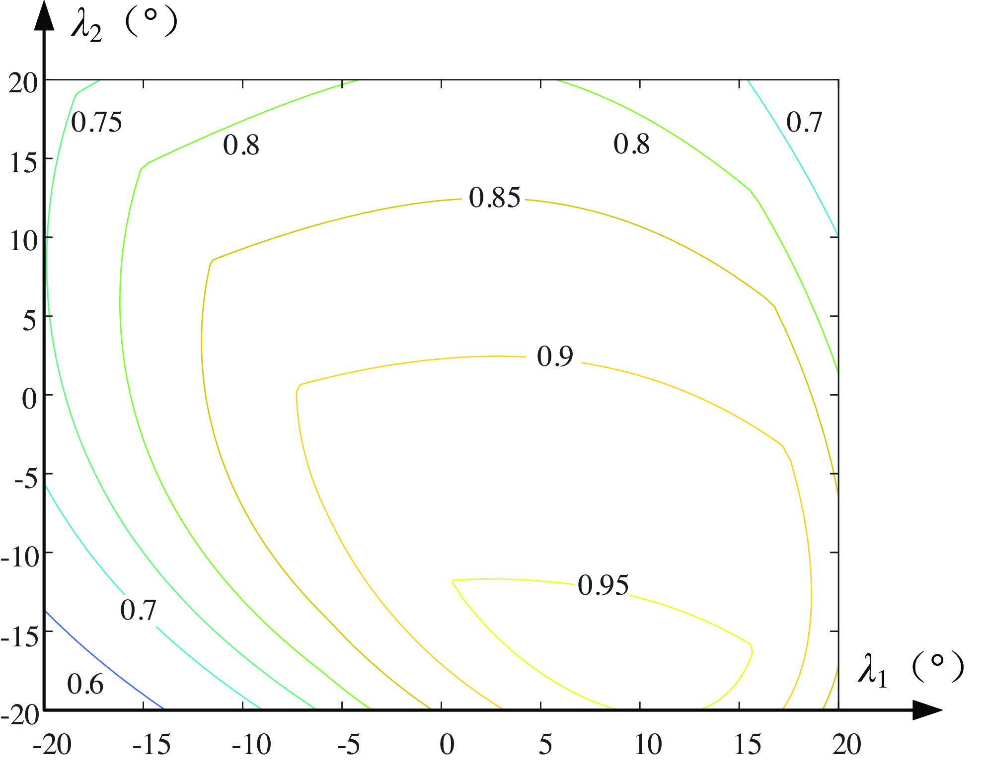
The LTI contour of the parallel rehabilitative mechanism is shown with λ 1 and λ 2 as coordinates, as depicted in Fig. 12.
Contour of local transmission index.

Figure 12 illustrates that the mechanism exhibits commendable transmission capabilities, with the majority of its transmission efficiency indexes exceeding the 0.5 threshold across various areas. A value of LTI below 0.1 suggests the presence of a transmission singularity. The depicted graph’s lowest LTI is 0.3, which denotes that the mechanism is well-removed from any transmission singular state. In instances where λ 1 drops below zero, the transmission efficacy is enhanced, implying that the left segment of the LTI map excels over the right. Similarly, if λ 2 falls below zero, the transmission quality is superior, meaning the bottom section outperforms the top. In general, as the inclination angle of the mechanism increases, its transmission efficiency tends to decline.
4.3. Constraint performance analysis
The input constraint performance index
 $k_{Ii}$
signifies the efficiency ratio connecting the constraint wrench screw
 $\boldsymbol{\$ }_{i}^{r}$
, subject to the branch restriction, and the branch’s restricted twist screw
 $\boldsymbol{\$ }_{Ri}$
. Meanwhile, the performance index
 $k_{Oi}$
, representing the output constraint index, denotes the efficiency ratio linking the constraining force
 $\boldsymbol{\$ }_{i}^{r}$
applied on the branch and the moving platform’s restricted twist screw
 $\bigtriangleup \boldsymbol{\$ }_{Oi}$
. Comparably, the following is the definition of the local constraint index (LCI):
 \begin{equation}k=\min \left(k_{Ii},k_{oi}\right) \end{equation}
In like manner, the LCI map illustrating the mechanism is constructed using the human body’s angular displacement λ 1 at the tibiotalar joint and the angular displacement λ 2 at the subtalar joint as its reference coordinates, as depicted in Fig. 13.
Contour of local constraint index.

Figure 13 illustrates that the mechanism exhibits excellent constraint performance, with the majority of its constraint efficiency indexes exceeding the 0.8 threshold across various areas. A value of LCI below 0.1 suggests the presence of a constraint singularity. The depicted graph’s lowest LCI is 0.6, which denotes that the mechanism is well-removed from any constraint singular state. In instances where λ 1 greater than zero, the constraint efficacy is enhanced, implying that the right segment of the LTI map excels over the left. Similarly, if λ 2 greater than zero, the constraint quality is superior, meaning the upper section outperforms the bottom. In general, as the inclination angle of the mechanism increases, its constraint efficiency tends to enhance.
4.4. Workspace analysis
The analysis of the workspace for an ankle rehabilitative robot is essential to meet training needs, covering all required ankle ranges of motion. It is crucial to ensure that the robot’s workspace is sufficient to replicate all ankle movements, including dorsiflexion/plantarflexion, varus/valgus, and adduction/abduction. The Tilt-and-Torsion Euler angle is used to assess the 3D orientation workspace of the rehabilitative mechanism, with the T&T attitude represented by three parameters: α (azimuth angle), β (tilt angle), and γ (torsion angle).
 \begin{align}{}^{O}{\boldsymbol{R}}{_{P}^{}} & =\boldsymbol{R}_{z}\left(\alpha \right)\boldsymbol{R}_{y}\left(\beta \right)\boldsymbol{R}_{z}\left(-\alpha \right)\boldsymbol{R}_{z}\left(\gamma \right) \nonumber\\ & =\left[\begin{array}{l@{\quad}l@{\quad}l} c\alpha \cdot c\beta \cdot c\left(\gamma -\alpha \right)-s\alpha \cdot s\left(\gamma -\alpha \right) & -c\alpha \cdot c\beta \cdot s\left(\gamma -\alpha \right)-s\alpha \cdot c\left(\gamma -\alpha \right) & c\alpha \cdot s\beta \\ s\alpha \cdot c\beta \cdot c\left(\gamma -\alpha \right)+c\alpha \cdot c\left(\gamma -\alpha \right) & -s\alpha \cdot c\beta \cdot s\left(\gamma -\alpha \right)+c\alpha \cdot c\left(\gamma -\alpha \right) & s\alpha \cdot s\beta \\ -s\beta \cdot c\left(\gamma -\alpha \right) & s\beta \cdot s\left(\gamma -\alpha \right) & c\beta \end{array}\right] \end{align}
where,
 $s\beta =\sin \beta, c\beta =\cos \beta$
, and
 $c(\gamma -\alpha )=\cos (\gamma -\alpha ),\,s(\gamma -\alpha )=\sin (\gamma -\alpha )$
.
The workspace of a parallel rehabilitative robot with a given size is influenced by multiple limitations. The following four limitations are particularly critical:
 $\unicode{x2460}$
The stroke range of the driving joint, and the stroke range of the drive joint (usually a linear actuator) directly determine the maximum and minimum displacements that the parallel robot can produce;
 $\unicode{x2461}$
Rotating angle range of the passive joint, although the passive joint is not directly driven by the motor, its rotation angle range still limits the workspace of the robot;
 $\unicode{x2462}$
Collision and interference between the branches, the collision will not only limit the workspace but also cause damage to the mechanism. When designing, it is necessary to consider the layout and trajectory of the branched chain to avoid such interference;
 $\unicode{x2463}$
Kinematic singularity of mechanism, kinematic singularity refers to the situation in which a robot loses or adds one or more degrees of freedom under certain specific positioning shapes. The mathematical formulation of the workspace constraints of the rehabilitative mechanism is as follows:
 \begin{equation}\left\{\begin{array}{c} l_{\min }\leq l_{i}\leq l_{\max }\\ q_{i}\leq q_{\max }\\ D\leq D_{ij}\\ \min \left(\lambda, k\right)\geq 0.1 \end{array}\right. \end{equation}
In the expression, l max and l min stand for the maximal and minimal values of the stroke of the electric cylinder in the driving branch, respectively. q max is the maximal rotation range of the passive rotating joint in each branch of the mechanism (mainly for the rotation angle limit of the spherical joint). D represents the maximum diameter of the connecting rod in the branch. D ij represents the minimum distance between the branches. The value of min (λ, k) represents whether the mechanism belongs to the singular state. When min (λ, k) is less than 0.1, it can be considered that the mechanism is in a singular state. min (λ, k) is the minimal value of the transmissibility index and the constrainability index of the parallel rehabilitative mechanism.
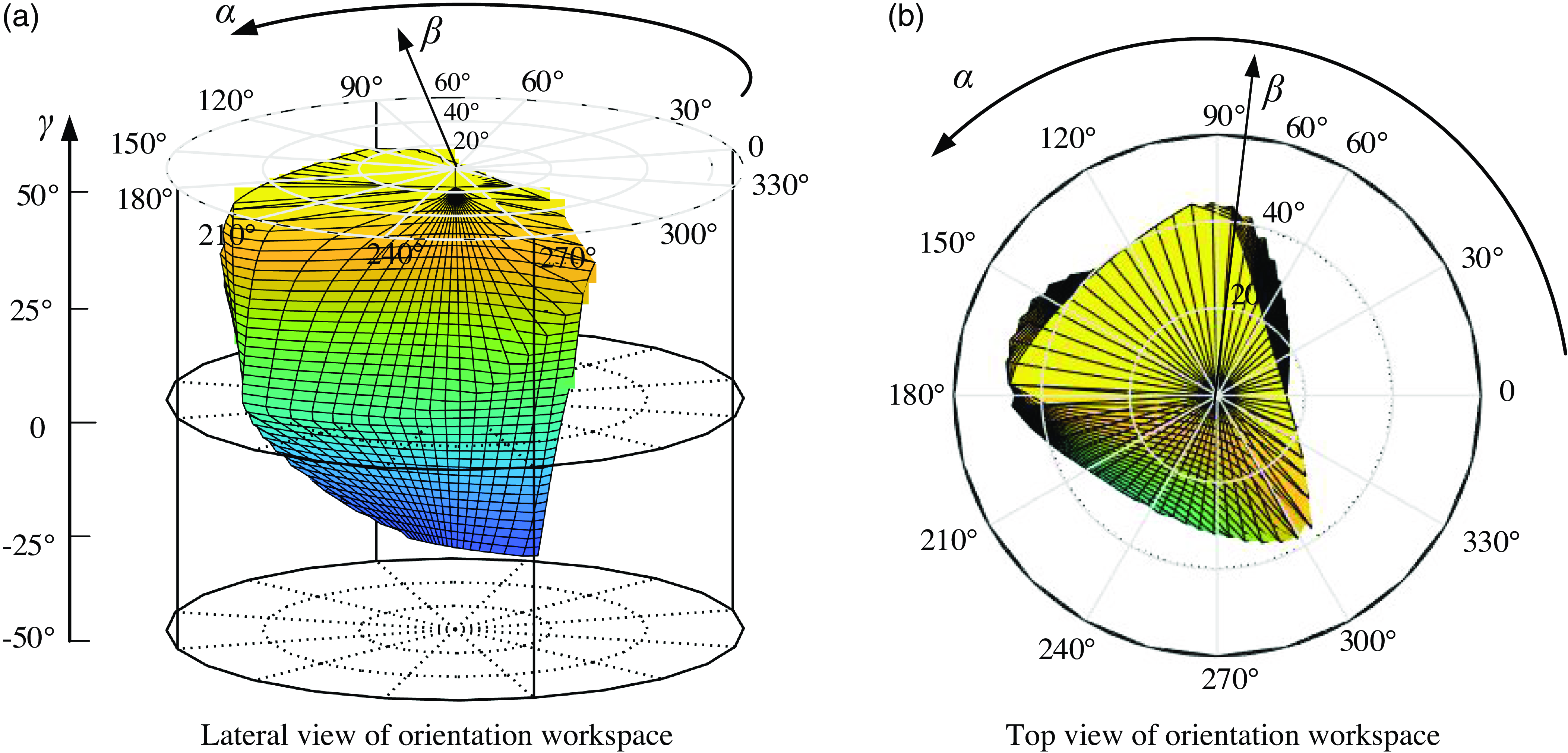
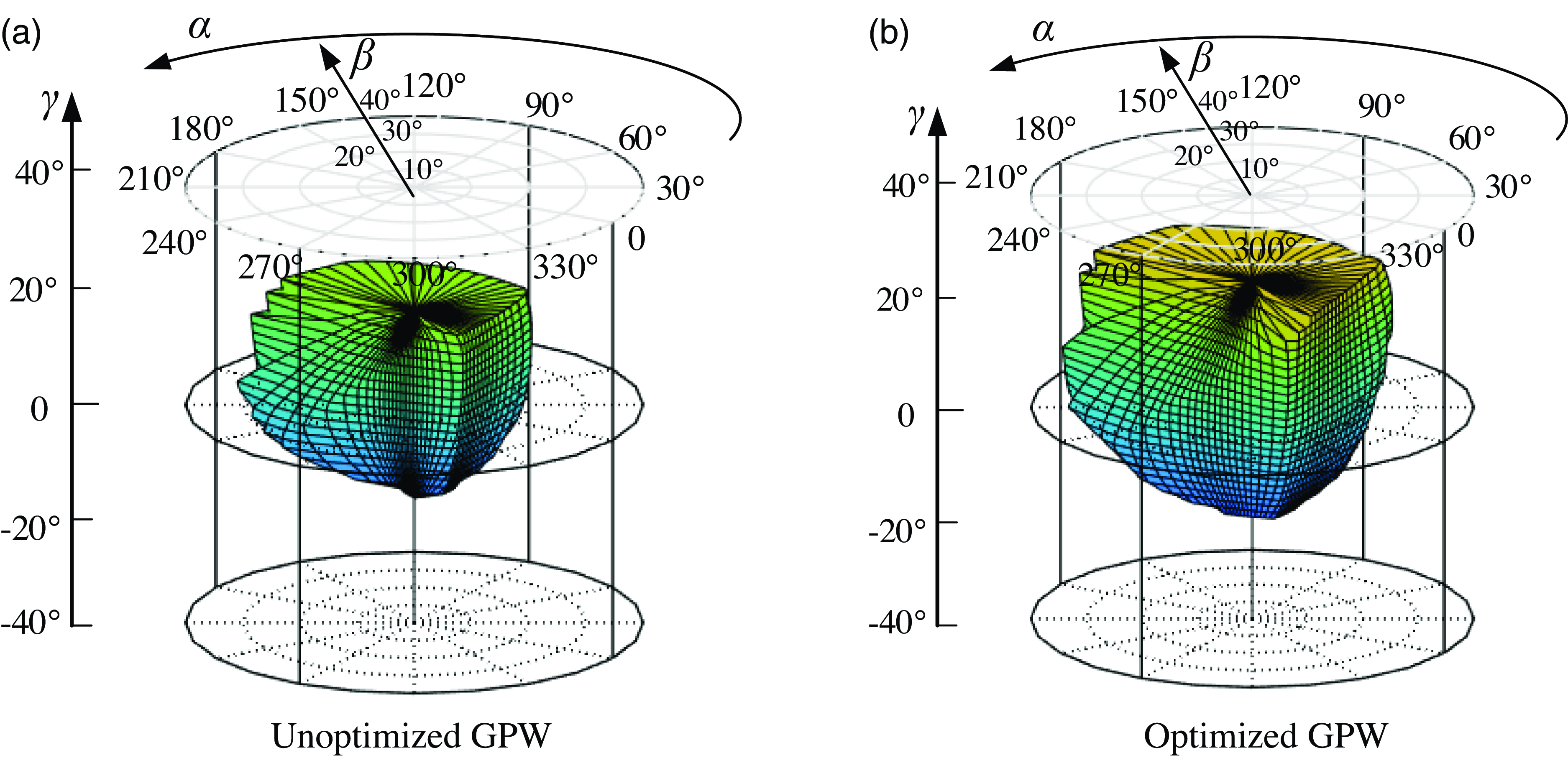
The boundary search method is used to analyze the workspace of the rehabilitative mechanism, define the structural parameters and geometrical restriction of the mechanism, set the search range and step size, and record all the boundary points of the workspace in combination with the inverse kinematics model of the rehabilitative mechanism for drawing. The size parameters of the mechanism are consistent with those mentioned in Section 4.2. When l max = 400 mm, l min = 240 mm, and D = 30 mm, q max = 20°, the rotational range of the rehabilitative mechanism can be explored. The circular cylindrical coordinates framework is employed to express the orientation workspace of the rehabilitative mechanism, as depicted in Fig. 14. Any point in the posture space of the rehabilitative mechanism can be defined by angle α, radial distance β, and height γ.
Rehabilitative mechanism rotational workspace.

From Fig. 14(a), it is evident that the rehabilitative robot demonstrates good rotation performance, achieving a range of [-25°, 45°] in adduction/abduction mode, meeting the required range of motion (ROM) of the human mortise-joint. In Fig. 14(b), the robot achieves a range of [-35°, 42°] in dorsal extension/plantar flexion mode and [-45°, 18°] in varus/valgus mode, also meeting the human ankle joint ROM requirements.
5. Dimension optimization of rehabilitative mechanism
5.1. Local design index
For an integrated parallel manipulator, it is indispensable and sensible to take the entire manipulator, including both transmission and constraint performance, into account when evaluating the kinematic performance. Therefore, a local design index (LDI) is specified as:
 \begin{equation}\mathrm{LDI}=\min \left\{\lambda, k\right\} \end{equation}
5.2. Global design index
Furthermore, to evaluate the global transmission/constraint performance of mechanisms, the good-performance workspace (GPW) is defined. GPW [Reference Song, Zhao, Zhao, Yan and Chen39] is the workspace where the LDI of every point is no smaller than 0.7. Within the GPW, the mechanism has good performance and gets away from its singular configurations [Reference Xu, Li, Zhang and Chen40]. Then, the global design index (GDI) over the entire GPW is defined as
 \begin{equation}\mathrm{GDI}=\int \frac{\mathrm{LDI}\cdot \mathrm{dW}_{1}}{\mathrm{LDI}\cdot \mathrm{dW}_{2}} \end{equation}
Where W1 is the workspace where the LDI value of every point is not less than 0.8, and W2 is the workspace where the LDI value of every point is not less than 0.7. It can be seen from the above formula that the global performance index (GPI) [Reference Song, Zhao, Zhao, Yan and Chen39] represents the ratio of the workspace whose LDI value is greater than or equal to 0.8 in its GPW. The higher the GDI value, the better the transmissibility and the constrainability of the mechanism in its GPW.
5.3. Dimensional synthesis
To make the rehabilitative mechanism have better transmissibility and constrainability, the size optimization design of the rehabilitative mechanism is carried out with the goal of larger GPW and GDI index values. The size parameters needed to be optimized are a, b, and r. First, dimensionless processing of dimension parameters:
 \begin{equation}D=\left(a+b+r\right)/3,r_{1}=b/D,r_{2}=r/D,r_{3}=a/D \end{equation}
According to the geometric constraints of the mechanism itself:
 \begin{equation}\left\{\begin{array}{l} 0\lt r_{1},r_{2},r_{3}\lt 3\\ r_{1}+r_{2}+r_{2}=3\\ r_{2}\lt r_{1}\lt r_{3} \end{array}\right. \end{equation}
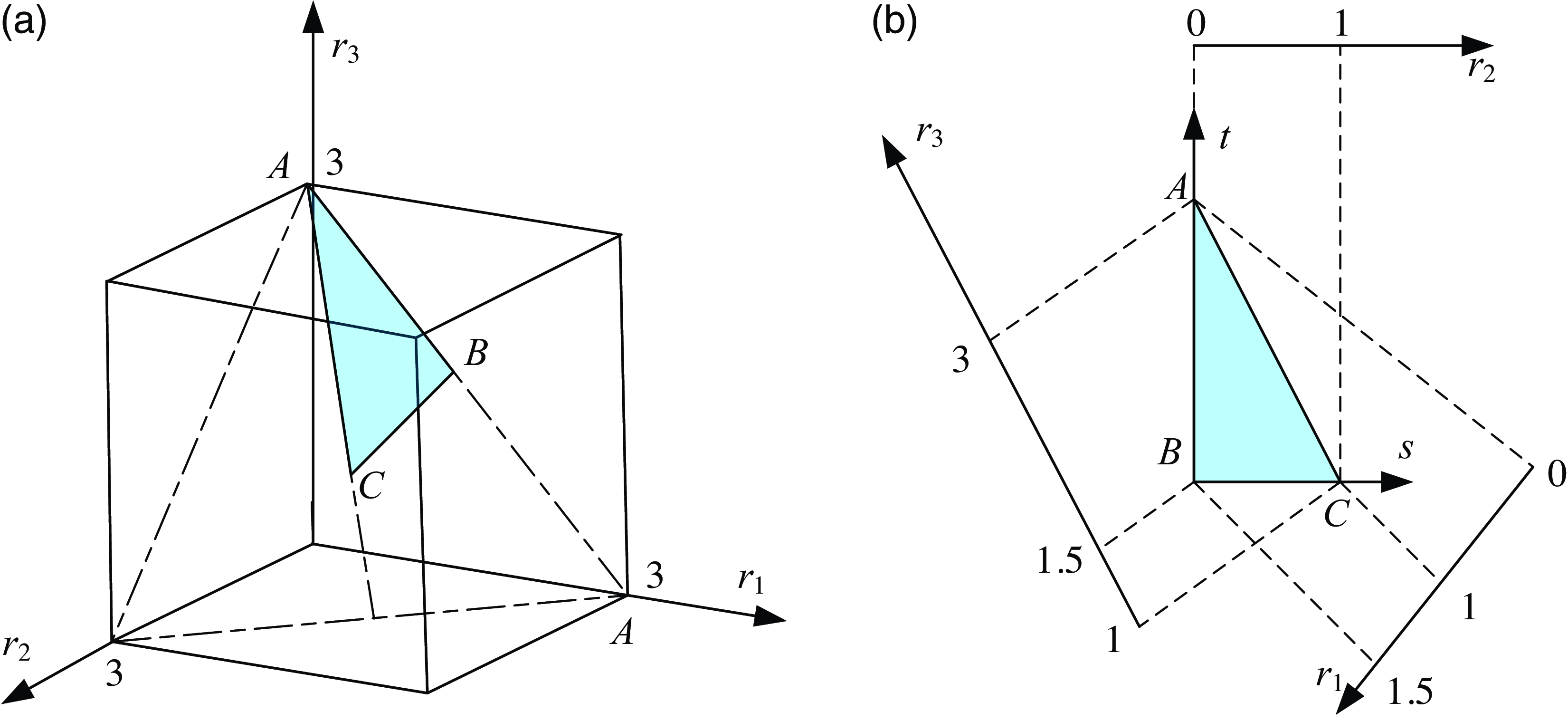
By Eq. (24), with r 1, r 2, r 3 as coordinate axes respectively, a plane area ABC, that is, the parameter design space of the ankle rehabilitative mechanism can be determined, as shown in the shadow area in Fig. 15(a). In this parameter design space, each point represents a set of size parameters of the mechanism. Through this parameter design space, the relationship between the optimization index and the geometric size parameters of the mechanism can be established.
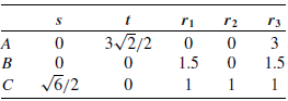
As depicted in Fig. 15(b), the parameter design space can be expressed as a two-dimensional form. There are the following data relations between (r 1, r 2, r 3) and (s, t).
It can be seen from Table 1 that the relationship between (r 1, r 2, r 3) and (s, t). is as follows:
The position coordinates of plane area ABC.

 \begin{equation}\left\{\begin{array}{l} r_{1}=-\frac{\sqrt{6}}{6}s-\frac{\sqrt{2}}{2}t+1.5\\ r_{2}=\frac{\sqrt{6}}{3}s\\ r_{3}=-\frac{\sqrt{6}}{6}s+\frac{\sqrt{2}}{2}t+1.5 \end{array}\right. \end{equation}
Parameters design space of the rehabilitative mechanism.

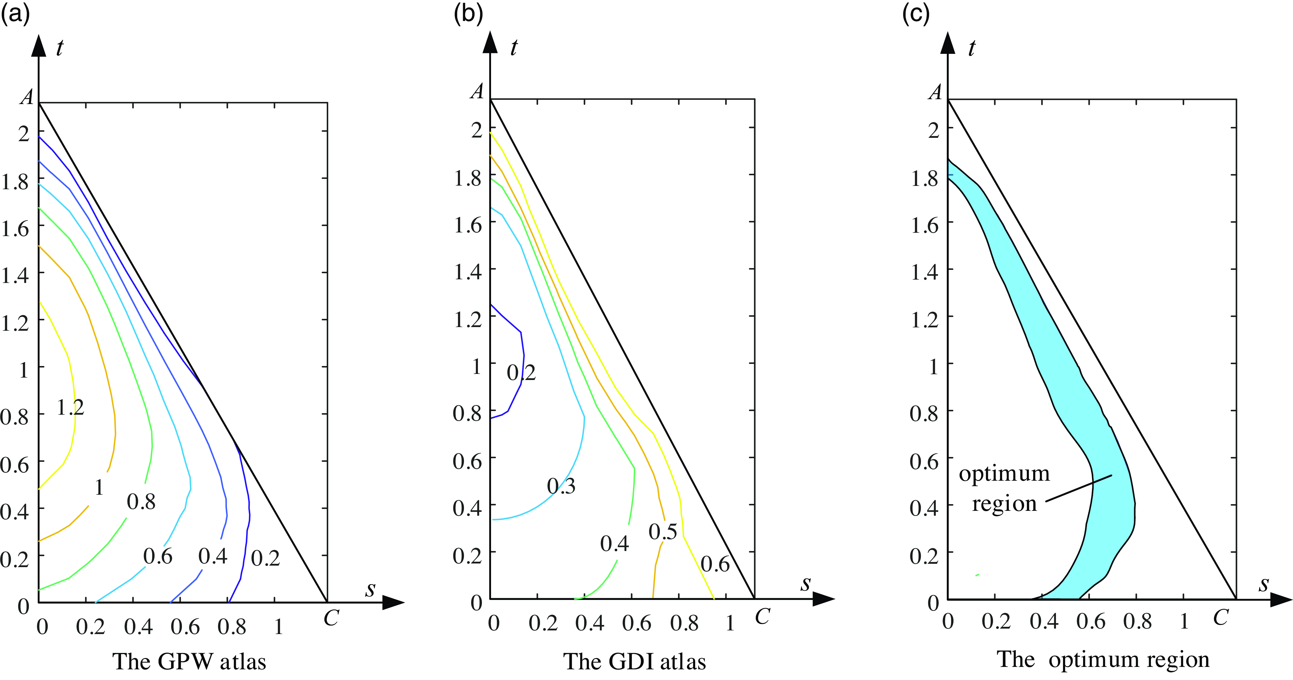
According to the definition of GPW and GDI, the optimal design atlas of rehabilitative mechanism in parameter design space is shown in Fig. 16.
Optimal design atlas.

The graph in Fig. 16 shows that the GPW value decreases as s increases, while the GDI value increases with s. To enhance motion transmission, constraint performance, and rotation capacity of the mechanism, maximizing GPW and GDI is essential. Thus, selecting the intersection of GPW≥0.4 in Fig. 16(a) and GDI≥0.4 in Fig. 16(b) defines the optimal design area for the ankle rehabilitative mechanism, depicted by the shaded region in Fig. 16(c).
Select design parameters for the rehabilitative mechanism in the optimal region of Fig. 16(c), for example, s = 0.7, t = 0.5. Using Eq. (23): r 1 = 0.86, r 2 = 0.57, r 3 = 1.57. By combining Eq. (21) with D = 100 mm, it is determined that b = 86 mm, r = 57 mm, and a = 157 mm, representing the optimal design dimensions of the rehabilitative mechanism. The GPW of the rehabilitative robot post-scale optimization is depicted in Fig. 17 (b). At this scale, OpenSim biomechanical software validates the rehabilitative robot’s effectiveness.
Rehabilitative mechanism good-performance workspace.

6. Human-robot coupling rehabilitative simulation
As a rehabilitative medical apparatus, a rehabilitative robot assists patients in safe and comfortable therapy, requiring evaluation of its effectiveness. Biomechanical analysis software, like OpenSim [Reference Liu, Dimitrov, Jomha, Adeeb, El-Rich and Westover41], is commonly used to assess the impact of rehabilitative robots owing to the intricacy of human bone structures and joints. OpenSim simulates musculoskeletal dynamics and neuromuscular control, offering precise models for muscle dynamics and joint kinematics.
Rehabilitative therapy modes are categorized as passive, collaborative, and active, depending on the patient’s injury level [Reference Choi, Won, Lee and Park42]. Passive therapy is used in the early stages when the limb may not respond [Reference Washabaugh, Guo, Chang, Remy and Krishnan43]. Collaborative therapy involves both the patient and the rehabilitative robot moving together in the middle stages [Reference Blank, French, Pehlivan and O’Malley44]. Active rehabilitative therapy, using impedance, is conducted in the later stages when the patient has regained muscle strength [Reference Zheng, Shi, Fan, Liang, Li and Yu45].
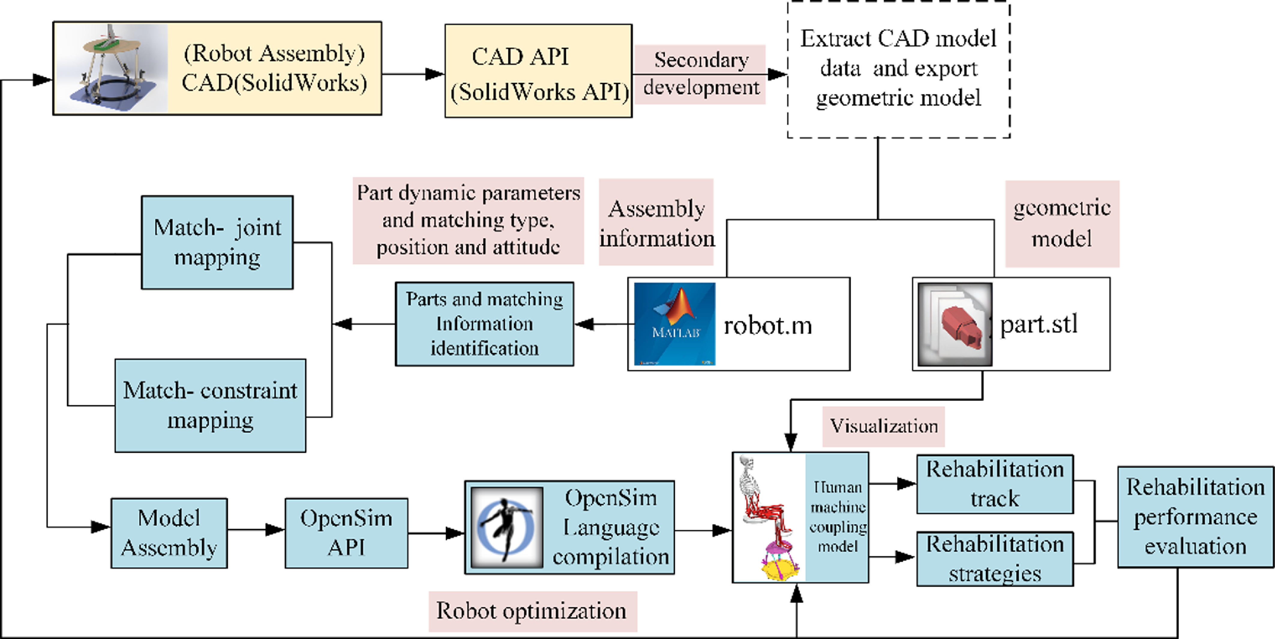
Firstly, the 3-D model of the rehabilitation robot is constructed by means of CAD modeling software. Then, based on the OpenSim biomechanical software, the ankle neuromuscular skeleton model was established, and the human body model containing this neuromuscular skeleton was combined with the rehabilitation robot to build a human-machine coupling simulation model. Finally, according to the human-machine coupling model, the rehabilitation simulation is carried out according to different rehabilitation trajectories and rehabilitation strategies in the biomechanical software. At the same time, according to the measured values of the maximum joint force, the maximum muscle force, the maximum muscle stress, and the muscle activation degree of the human joint, the rehabilitation performance indexes such as safety and comfort of the rehabilitation robot are constructed, and the design-evaluation-optimization system of the rehabilitation robot is further established. Finally, a simulation verification platform for the development and design, performance evaluation, multi-objective optimization, and rehabilitation strategy optimization of the rehabilitation robot is built. The detailed technical route can be shown in Fig. 18.
Using the API interface of CAD software, the secondary development is carried out. The part information and matching information of the robot model are automatically extracted and the STL format geometric model is automatically derived. The extracted data information is saved as the m file supported by MATLAB, which contains the dynamic parameters such as part mass, centroid coordinates, and the assembly information such as the matching relationship and the homogeneous transformation matrix of parts. Identify the extracted match relationship in MATLAB software, such as coincidence, distance, concentricity and other match types and match positions, and equivalent it to the kinematic constraints supported by OpenSim software. Then, based on the homogeneous transformation matrix of parts and the theory of robot mechanism, the local coordinate system of each joint can be established, and then the assembly model of robot can be constructed. The robot model is coupled with the human neuromusculoskeletal model by means of motion constraints, flexible forces, and contact, and the human rehabilitation mechanical coupling model is established.
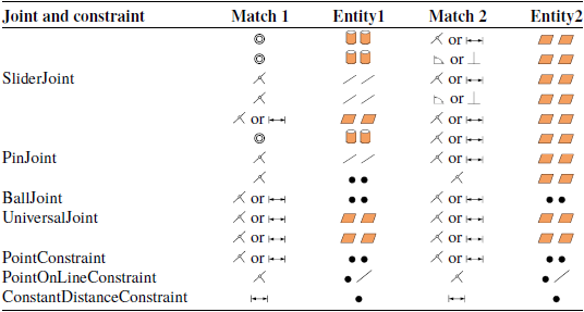
In SolidWorks assemblies, parts are connected using match relationships rather than kinematic pairs. Each match carries out motion constraints between mating entities on different parts. Matches include parallel, concentric, coincident, and distance types. Mating entities include points, lines, and faces. The supported match types and match entities are defined, as shown in Table 2.
Human-machine coupling simulation technology roadmap.

SolidWorks match type and match entity.

In OpenSim software, the function of joint and constraint module can be equivalent to the coordination function in SolidWorks software. Their main responsibility is to clarify the kinematic constraints between the two entities. As for the specific mapping relationship among fit, kinematic pair, and constraint, see Table 3 for details.
Match - joint/constraint mapping relationship.

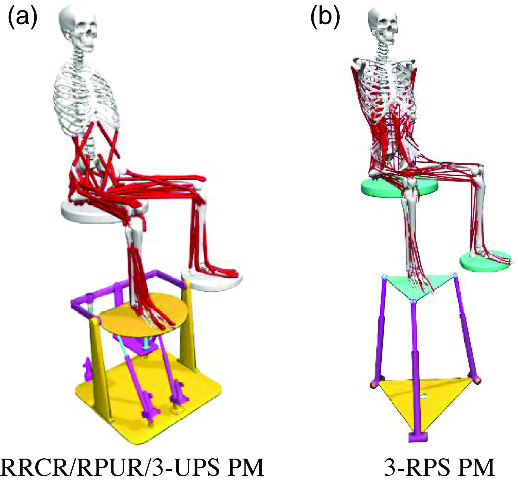
Through the joint and constraint mapping theory, the cooperation relationship in SolidWorks is automatically transformed into the joint and constraint relationship of the kinematic joint supported by OpenSim; Through the matching position information extracted from SolidWorks API interface and the homogeneous transformation matrix of each part, the position and posture of each joint coordinate system in two adjacent parts are obtained, and then the joint coordinate systems are established to automatically assemble and connect the robot system. Bushingforce is used to simulate the flexible bandage to couple the robot model and the manikin, as shown in Fig. 19, which are the proposed rehabilitation robot and the typical 3-RPS ankle rehabilitation robot.
Human-robot coupling rehabilitation simulating model.

Using the human-robot coupling model established above, we conducted passive rehabilitation simulations on patients in the early rehabilitation stage of ankle joint injuries. The robot actively moves the human ankle to perform inversion/eversion and dorsiflexion/plantar flexion, while the human ankle muscle passively stretches in response. The specific motions of the tibiotalar and subtalar joints are as follows:
 \begin{equation}\left\{\begin{array}{l} \lambda _{1}=\frac{\pi }{10}\cdot \sin \left(0.5\pi t\right)\\ \lambda _{2}=\frac{\pi }{12}\cdot \sin \left(0.5\pi t\right) \end{array}\right. \end{equation}
The primary movement of foot articulation is governed by the lower limb’s muscular structure. In the processes of foot dorsiflexion and plantar flexion, along with the inward and outward movements known as inversion and eversion, the principal muscles involved are the extensor digitorum longus, tibialis posterior, tibialis anterior, flexor digitorum longus, extensor hallucis longus, flexor hallucis longus, soleus, gastrocnemius, and peroneus brevis. These particular muscles were pinpointed as the main subjects for the analytical study. Key metrics such as muscle activation levels, passive resistance, muscle fiber lengths, and the reactive forces at the ankle joint were determined as the critical output variables to gauge the efficacy of the therapeutic robot in rehabilitation.
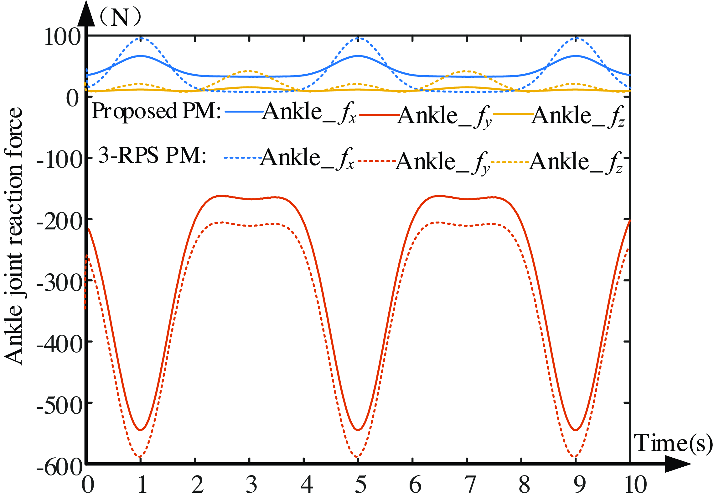
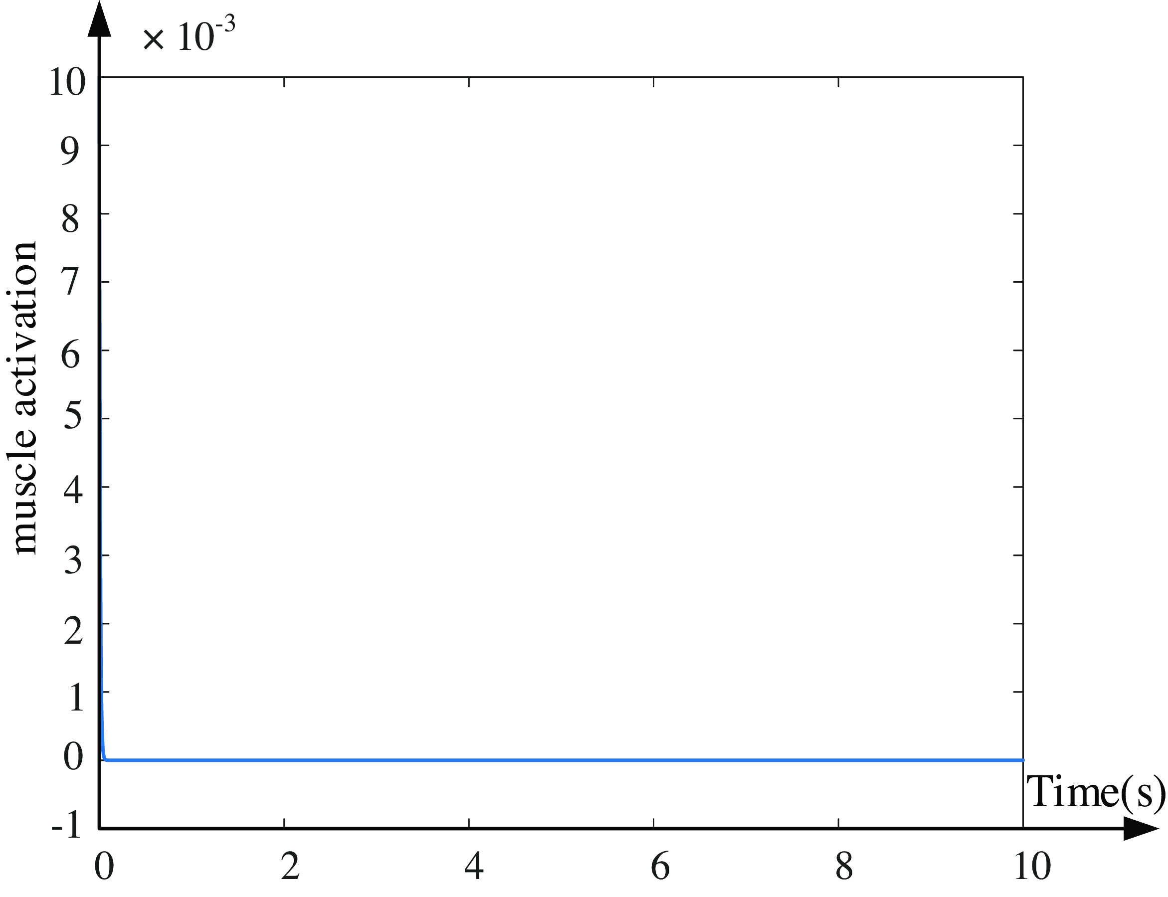
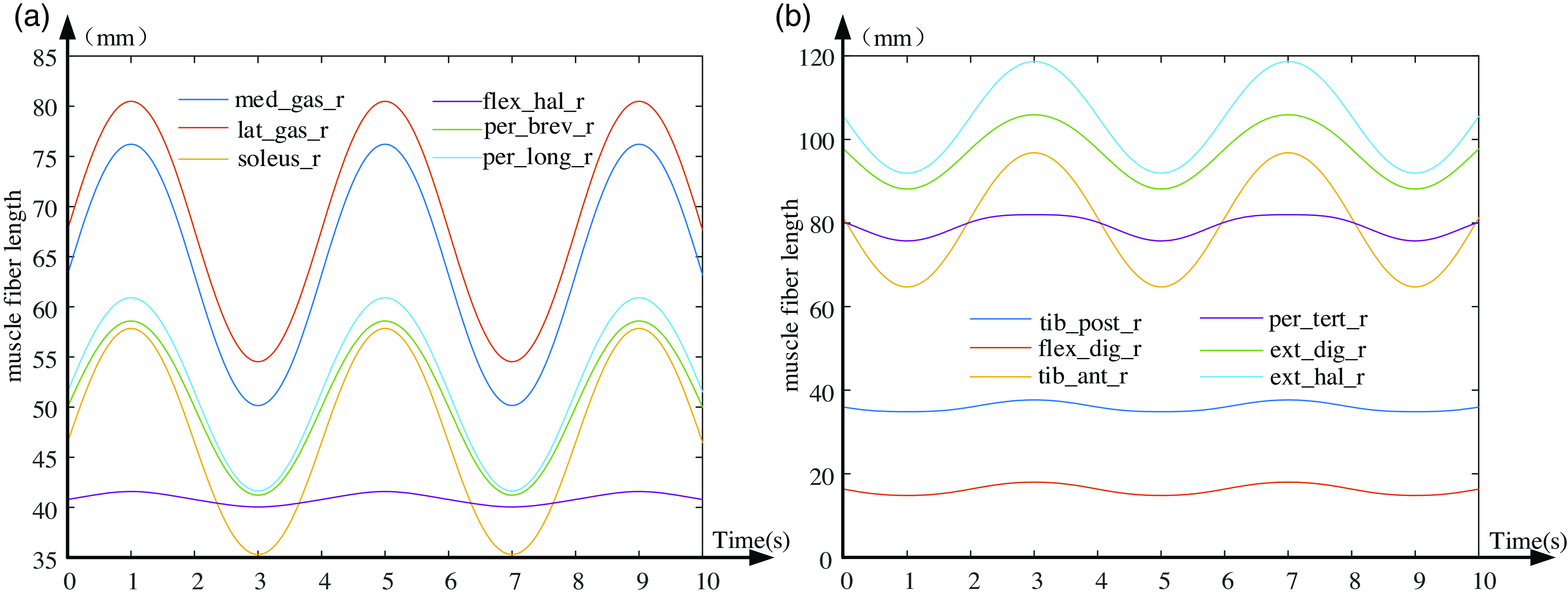
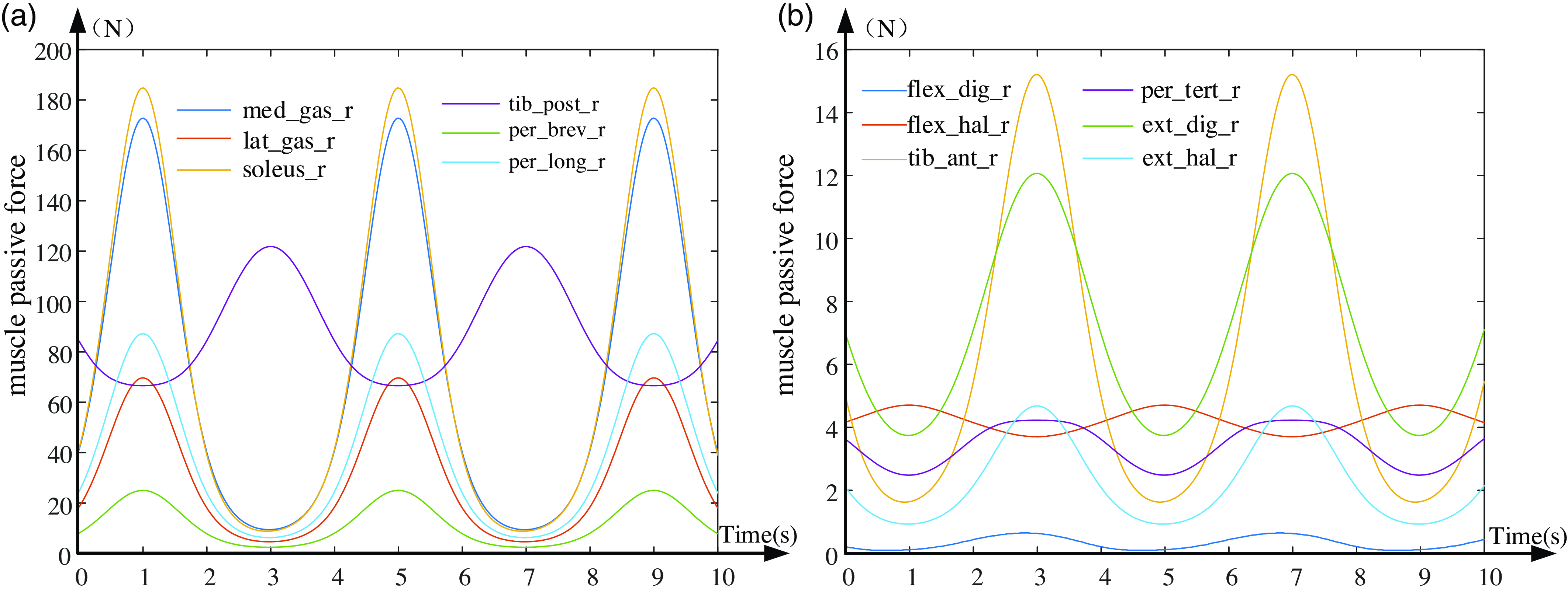
During the rehabilitative process, it is crucial to prevent a sharp increase in muscle force to avoid discomfort in the foot and to ensure that the ankle joint reaction force and muscle fiber length curves do not exhibit abrupt fluctuations. When conducting rehabilitative therapy following the trajectory defined by Eq. (26), the ankle joint reaction force curve between the foot and the shank is depicted in Fig. 20; muscle activation levels are shown in Fig. 21; muscle fiber lengths are illustrated in Fig. 22; and passive tensions are presented in Fig. 23.
The ankle joint reaction force curve.

Ankle muscle activation curve.

Human ankle muscular fiber length variation curves.

Human ankle muscular passive force variation curves.

From Fig. 20, the maximal contact force at the ankle joint is in the y-direction, with a peak value of about 550 N. This is followed by the force in the x-direction, peaking at around 80 N along the foot direction (X-axis). The force in the z-direction is minimal in this trajectory. The joint force curve is consistently smooth in all directions, without any abrupt changes or fluctuations, ensuring comfort and safety for the foot. Figure 21 indicates a muscle activation degree of 0, suggesting passive stretching without active force generation, aligning with the patient’s initial passive rehabilitative. Figure 22 illustrates a smooth transition of the ankle joint’s muscle fiber length curve under this rehabilitation trajectory in Eq. (26), avoiding sudden elongation and patient discomfort. Under this recovery path, the muscle length variation curves shown in Fig. 22(a) show an accordant trend, indicating that these muscles are synergistic. Likewise, the muscles in Fig. 22(b) also exhibit synergistic behavior. However, the muscle length variation curves in Figs. 21(a) and 22(b) display contrary variation trends, indicating these muscles are antagonistic. From Fig. 23, it is evident that five muscles – tibialis posterior (tib_post_r), soleus (soleus_r), peroneus longus (per_long_r), medial gastrocnemius (med_gas_r), and peroneus brevis (per_brev_r) – experience the highest force, while other muscles undergo minimal tension. The maximum tension on any muscle does not surpass 200 N, and the muscle curves transition smoothly without sudden spikes. This prevents secondary damage to the ankle joint and ensures comfort during the rehabilitation process. Through the in-depth analysis of the above simulation results, it can be found that under the same trajectory conditions, the ankle rehabilitation mechanism proposed in this paper is compared with the typical 3-RPS parallel rehabilitation mechanism. Under the same trajectory, the muscle stimulation effect of the two mechanisms is exactly the same. However, there are differences in the force applied to the ankle joint. The force applied to the ankle joint by the rehabilitation institution proposed in this paper is significantly smaller. Especially in the non-freedom direction of the ankle joint, the force generated by the rehabilitation mechanism is relatively small. This feature means that in the process of practical application, it will not exert a large tension on the ligament of the ankle joint, so the rehabilitation institution has better comfort and higher safety, and can provide more favorable conditions for the rehabilitation treatment of patients.
7. Conclusions
This investigation focused on crafting an equivalence model for the ankle rehabilitation robot, inspired by the human ankle’s anatomical framework and kinetic characteristics. The correlation between the human ankle’s movement and the rehabilitation mechanism’s configuration design was meticulously defined. To initiate, an innovative 4-DOF ankle rehabilitation device, featuring three rotations and a translation, was engineered. This device incorporates dual virtual motion centers and boasts benefits such as synchronized human-robot motion, versatility for various patient needs, ease of donning, interchangeability between right and left feet, and enhanced safety measures. Secondly, based on the motion properties of parallel rehabilitative mechanism, it was equivalent to a series RCR mechanism, and then using DH (Denavit-Hartenberg) method, the kinematic inverse solution of parallel rehabilitative mechanism was constructed. Thirdly, by examining the motion/force transmissibility and the constrainability, a thorough assessment of the mechanism’s kinematic capabilities and operational range was conducted. It was demonstrated that the therapeutic mechanism exhibits superior transmissibility and constrainability, along with an ample workspace. Then, taking a, r, b as the optimization parameters, the dimension synthesis of the mechanism was executed, and a set of optimal scale combinations of rehabilitative mechanisms were determined. Finally, utilizing the OpenSim biomechanical tool, we crafted an integrated human-robot rehabilitation simulation framework. The efficacy of the rehabilitation process was assessed by analyzing the change curves of the ankle joint reaction force, the lengths of muscle fibers, and the passive tension within the muscles. This study provides pivotal insights for devising rehabilitation tactics in a passive therapy context and paves the way for future development of a physical prototype and its kinematic control.
Author contributions
Jianjun ZHANG was in charge of the whole research; Jingke SONG wrote the manuscript; Jun WEI assisted with the analysis and validation; and the remaining discussed and read the manuscript. All authors read and approved the final manuscript.
Financial support
This research work was funded by the National Natural Science Foundation of China (Grant Numbers 52075145), the Science and Technology Program of Hebei Province (Grant Numbers 20281805Z), and the Central Government Guides Basic Research Projects of Local Science and Technology Development Funds (Grant Numbers 206Z1801G), the National Natural Science Foundation of China Grant Numbers 52405015, China Postdoctoral Science Foundation Funded Project (Grant Numbers 2024M760729).
Conflicts of interest
The authors declare no conflicts of interest exist.
Ethical approval
Not applicable.
Supplementary material
The supplementary material for this article can be found at https://doi.org/10.1017/S0263574725000128.