NOMENCLATURE
- Aref
-
reference relation area of the HIRENASD wing Aref = 0.393m 2
- aG i
-
response of the Gaussian RBF to the ith sample point
- aIQ i
-
response of the IQ RBF to the ith sample point
- c 4-7
-
chord length of cut 4 through 7
- CD
-
drag coefficient
- CL
-
lift coefficient
- CM
-
pitching moment coefficient
- e
-
time window size of grid velocities
- fsp
-
sparsing factor
- LRe
-
Reynolds length LRe = 0.3445m
- k
-
elliptic shape exponent
- Minp
-
number of input POD base vectors
- Mout
-
number of output POD base vectors
- N
-
number of RBFs
- p
-
dimension of system snapshot
 $\underline{y}$
- p ∞
-
free stream pressure
- q
-
number of system snapshots
$\underline{y}$
- qs (t)
-
generalised coordinate of the sth eigenmode
- r
-
fixed radius used for all radial basis functions
- ri
-
adaptive radius of radial basis function i
- s
-
number of training samples
-
$\text{M}$
-
Mach number
-
$\text{Re}$
-
Reynolds number
- U ∞
-
free stream velocity
- T ∞
-
free stream temperature
- t
-
time
- tpred
-
computational effort of the ROM for a prediction of the aerodynamic forces
- u z, Tip
-
tip node displacement in z-direction
- vtrunc
-
POD truncation threshold
- α
-
angle-of-attack
- θ y
-
torsion angle around y-axis
- θ y, Tip
-
tip node torsion angle around y-axis
- λ ii
-
eigenvalue of the ith POD mode (method of snapshots)
- λ s
-
smoothing factor
- ρ∞
-
free stream density
- σ i
-
singular value of the ith POD mode
-
${\underline{c}}_F$
-
normalised aerodynamic forces
-
$\hat{\underline{c}}_{F,i}$
-
POD coefficients of normalised aerodynamic forces of ith sample
-
$\underline{c}_i$
-
centre of ith radial basis function
-
$\underline{D}$
-
normalised average distance of all RBF centres in each dimension
-
${\underline{F}}_x$
-
aerodynamic forces in x-direction (on the fluid grid)
-
${\underline{F}}_z$
-
aerodynamic forces in z-direction (on the fluid grid)
-
$\underline{p}_{ref}$
-
reference point for CM calculation,
$\underline{p}_{ref}=(0.252,0.0,0.0)$
-
$\underline{u}$
-
fluid surface grid displacement vector
-
$\underline{u}^{f}(t)$
-
fluid surface grid displacement vector of the forced motion
-
$\underline{x}(t)$
-
mapping method input at time t
-
$\underline{\Phi }_s$
-
mode shape of the sth eigenmode
-
$\underline{\chi }_i$
-
ith POD mode
-
$\underline{\underline{\Sigma }}^{-1}$
-
inverse covariance matrix
-
$\underline{\underline{I}}^{i}$
-
identity matrix of dimension i, hence
$\underline{\underline{I}}^{i} \in \mathbb {R}^{i \times i}$
-
$\underline{\underline{\Sigma }}^*$
-
singular value matrix
-
$\underline{\underline{U}}^*$
-
left singular vector matrix
-
$\underline{\underline{V}}^*$
-
right singular vector matrix
-
$\underline{\underline{W}}$
-
weight matrix
-
$\underline{\underline{Y}}$
-
snapshot matrix
-
$\underline{\underline{\Lambda }}$
-
eigenvalue matrix


1.0 INTRODUCTION
Aeroelasticity is a challenging aspect in modern aircraft design. High-fidelity aeroelastic simulations with a computational fluid dynamics (CFD) solver coupled with a computational structure mechanics (CSM) solver lead to high computational costs. Thus, the application of such methods in the design process of an aircraft is still not practicable. Therefore, reduced order modeling (ROM) approaches for aeroelasticity problems have been developed since the last decade.
However, many different reduced order approaches exist, for instance harmonic balance, centre manifold, normal form and numerical continuation methods. Henshaw et al(Reference de C. Henshaw, Badcock, Vio, Allen, Chamberlain, Kaynes, Dimitriadis, Cooper, Woodgate, Rampurawala, Jones, Fenwick, Gaitonde, Taylor, Amor, Eccles and Denley1) give a good overview over these methods. According to Farhat(Reference Farhat2), the reduced order model approaches can be classified into two categories, the internal description and the external description. The idea of the internal description is to map the governing differential equations of a system into a low-dimensional subspace and to solve the reduced equation system subsequently. In contrast, the aim of the external description is the identification of an explicit input-output map that replaces the full-order system. This kind of model is often called the ‘black box model’.
An approach of the first category is the use of proper orthogonal decomposition (POD) for projection of the system into a low-dimensional subspace. For instance, Willcox et al(Reference Willcox and Peraire3) construct a linear reduced-order state space model via POD. Amsallem and Farhat(Reference Amsallem and Farhat4,Reference Amsallem, Cortial, Carlberg and Farhat5) show that new POD bases can be efficiently inter-polated from existing POD bases by using a tangent space of the Grassmann manifold. With this new POD base, a linear ROM at an inter-polated Mach number is created. Thomas et al(Reference Thomas, Dowell and Hall6) implemented the harmonic balance approach within the framework of a conventional CFD solver. According to this approach, the conservation variables are substituted by an Fourier expansion that allows to model non-linear un-steady aerodynamics for finite amplitude motions of a prescribed frequency. Chen et al(Reference Chen, Li and Yan7) use a flow solver-based non-linear POD approach for aeroelastic investigations.
In the second category, various system identification methods are used to create an input-output mapping, for instance the Kriging method, neural networks or support vector machines. An overview over these methods is given by Ahmed et al(Reference Ahmed and Qin8). Voitcu(Reference Voitcu and Wong9,Reference Voitcu and Wong10) applies multi-layer perceptron artificial neural networks (MLP-ANN) in aeroelastic systems with structural non-linearities. Lucia et al(Reference Lucia, Beran and Silva11) and Silva(Reference Silva12) consider first- and second-order Volterra theory for aerodynamic load prediction. Additionally, Lucia use the eigensystem realisation algorithm (ERA) to create a linear state-space formulation of the aerodynamic system from impulse excitations. Han et al(Reference Han, Zimmermann and Görtz13) show a multi-variable fidelity approach based on Kriging for an efficient approximation of static aerodynamic coefficients. Chen et al(Reference Chen, Zuo, Sun and Li14) utilise support vector machines for the prediction of limit cycle oscillations (LCO). Fagley et al(Reference Fagley, Seidel, Siegel and McLaughlin15) use POD in combination with wavelet neural networks (wavenet) to predict the non-linear dynamic behaviour of a free shear layer. Zhang et al(Reference Zhang, Wang, Ye and Quan16) show that radial basis function artificial neural networks (RBF-ANN) are able to predict LCO behaviour of the NACA64A010 aerofoil in the time domain.
The approach presented in this paper is also part of the second category and already described in Lindhorst et al(Reference Lindhorst, Haupt and Horst17). It is a comparable approach to Zhang(Reference Zhang, Wang, Ye and Quan16) but combined with POD to make it applicable for high-dimensional systems such as discrete 3D models. In Lindhorst et al(Reference Lindhorst, Haupt and Horst17), LCO behaviour of the NLR7301 aerofoil is predicted with the method.
This paper deals with the application of the method on the 3D HIRENASD configuration. The HIRENASD is designed to represent a modern transport aircraft wing. It is a multi-tapered, swept-back wing with a non-symmetric super-critical shape. The surrogate model is identified from transient RANS analyses, and consequently the influence of viscous effects on the aerodynamic forces is taken into account. It is shown that the surrogate model is able to replace the CFD solver without modifying the coupling environment and that a significant reduction of the computational effort can be achieved.
2.0 SURROGATE MODEL APPROACH
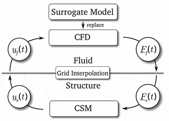
The surrogate model is dedicated to replace the CFD solver in an aerostructural coupling scheme (CFD-CSM scheme), see Fig. 1. In the current research, it is not the aerodynamic surface pressure but surface forces which are used for load transfer in the aerostructural coupling scheme.
Integration of surrogate model in the aerostructural coupling scheme.(Reference Lindhorst, Haupt and Horst17)

In a coupled aerostructural analysis, the CFD solver determines the flow field and the resulting discrete aerodynamic surface forces
 $\underline{F}_f(t)$
with respect to the discrete surface displacement
 $\underline{u}_f(t)$
. Consequently, the surrogate model must also predict the discrete force distribution
 $\underline{F}_f(t)$
on the aerodynamic grid from the discrete displacement vector
 $\underline{u}_f(t)$
of the aerodynamic grid surface. Thus, the surrogate model has to approximate relation 1.
 $$\begin{equation}
\underline{F}_f(t) = f(\underline{u}_f(t))
\end{equation}$$
In order to respect the influence of flow conditions on the aerodynamic forces, the dimensionless forces
 ${\underline{c}}_F$
are predicted by the ROM that are defined in accordance to the lift coefficient CL
:
 $$\begin{equation}
{\underline{c}}_F = \frac{\underline{F}_f}{\frac{1}{2}\rho _\infty U^2_\infty A_{ref}}
\end{equation}$$
Here, Aref
denotes the reference area, ρ∞ is the free stream density, and U
∞ is the free stream velocity. The reference area
 $A_{ref}=0.393\text{\,m}^2$
is a geometric parameter, and hence it is constant for an explicit aerodynamic configuration.
2.1 Process chain
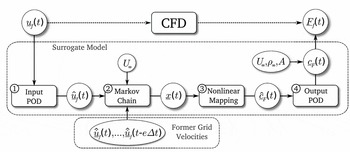
In order to approximate the high-dimensional, non-linear and time-dependent relationship given in Equation (1), a process chain is established that combines several methods in a modular manner. The process chain consists of four parts as shown in Fig. 2:
-
1. The input parameter reduction via POD (input POD)
-
2. The chronological rearrangement of the reduced grid displacements and velocities to the mapping method input vector
$\underline{x}(t)$
(Markov chain) -
3. The non-linear multiple input multiple output mapping (non-linear mapping)
-
4. The output parameter reconstruction via POD (output POD)

Scheme of the modular process chain for high-dimensional surrogate modeling.(Reference Lindhorst, Haupt and Horst17)

The parameter reduction via POD is explained shortly in Section 2.2. The composition of vector
 $\underline{x}(t)$
by using the Markov chain method is discussed in Section 2.3. For the non-linear mapping, any arbitrary mapping method can be chosen, for instance Kriging, support vector machines or artificial neural networks (ANN). In this paper, the radial basis function ANN is used, which is an easily implemented but effective method. A brief introduction to this method is given in Section 2.4. The modular characteristics make the surrogate model approach more variable. For instance, the Markov chain method can be switched off for time-independent problems or the POD reduction need not be used for low-dimensional systems.
All parts of the process chain are identified from known input-output training data of the full-order system. With this, the number of necessary sample points must be limited and the time used for the identification process should be as short as possible. The creation of training data and the identification of the model is discussed in Section 3.1.
2.2 Proper orthogonal decomposition
POD is also known as Karhunen-Loève expansion as well as principal component analysis (PCA). The idea of POD is to find a base of M orthogonal vectors for a given number of q snapshots
 $\underline{y}_1,\ldots ,\underline{y}_q$
of a field
 $\underline{y}$
of dimension p that is the optimal representation of the given snapshots.
For a time-dependent field
 $\underline{y}(t),$
the q snapshots are taken at different times
 $\underline{y}(t_1),\ldots ,\underline{y}(t_q)$
. The systems state
 $\underline{y}(t)$
is then represented by M time-dependent POD coefficients
 $\hat{y}_1(t),\ldots ,\hat{y}_M(t)$
and the identified M time-independent base vectors
 $\underline{\chi }_1,\ldots ,\underline{\chi }_M$
in sense of a linear combination (see Equation (3)).
 $$\begin{equation}
\underline{y}(t)= \underline{y}_0 + \sum ^M_{i=1} \hat{y}_i(t) \text{ } \underline{\chi }_i
\end{equation}$$
Here,
 $\underline{y}_0$
is a reference point defining the POD base origin in the high-order coordinate system. For more detailed information, the reader is referred to the plurality of publications about this method, for instance Lucia et al(Reference Lucia, Beran and Silva11), Willcox et al(Reference Willcox and Peraire3) or Meyer et al(Reference Meyer and Matthies18).
The base is constructed into a space spanned by known snapshots
 $\underline{y}(t_1),\ldots ,\underline{y}(t_q)$
of the system composed to a matrix
 $\underline{\underline{Y}}$
. The time-independent base vectors are determined by using singular value decomposition (SVD) applied on
 $\underline{\underline{Y}}$
.
 $$\begin{equation}
\underline{\underline{Y}} = \underline{\underline{U}}^* \underline{\underline{\Sigma }}^* \underline{\underline{V}}^*
\end{equation}$$
Here,
 $\underline{\underline{\Sigma }}^*$
is the singular value matrix containing the singular values σ
i
,
 $\underline{\underline{U}}^*$
are the corresponding left singular vectors, and
 $\underline{\underline{V}}^*$
is the corresponding right singular vectors. The left singular vectors equal the seeked POD base vectors. The POD base consists of q base vectors; hence, M = q. In order to reduce the dimension of the POD base, the base vectors
 $\underline{\chi }_i$
corresponding to small singular values σ
i
are truncated. A criterion for the truncation is defined in Equation (5).
 $$\begin{equation}
v=\frac{\sum ^M_i\sigma _i}{\sum ^q_j\sigma _j} \ge v_{trunc} \text{ }\text{ with }\text{ } 0.0 \le v_{trunc} \le 1.0
\end{equation}$$
The number of base vectors M < q is set in a way that equation v ⩾ vtrunc is satisfied. Here, vtrunc as a user defined threshold.
2.3 Markov chain model
In this section, the used Markov chain model is explained in brief. For detailed information, the reader is referred to the literature, for instance Meyn and Tweedie(Reference Meyn and Tweedie19).
The basic idea of a Markov chain model is the prediction of the current state of a time-dependent system from the finite history of former states. The system is considered as time discrete with a constant time step size Δt. Comparable approaches are utilised in surrogate modelling of aerodynamics such as the linear auto-regressive moving average (ARMA) model used by Won(Reference Won, Tsai, Sadeghi and Liu20) or the related auto-regressive with exogenous input (ARX) model used by Zhang(Reference Zhang, Wang, Ye and Quan16).
In this paper, grid displacements and velocities of the aerodynamic coupling surface are used as model input. In the Markov chain, the corresponding POD coefficients
 $\hat{\underline{u}}$
and
 $\hat{\dot{\underline{u}}}$
are used, not the full-order grid displacements
 $\underline{u}$
and velocities
 $\dot{\underline{u}}$
(see Equation (6)).
 $$\begin{equation}
\underline{x}(t) = \left(\underbrace{\underline{\hat{u}}(t)}_{\text{static part}}, \underbrace{\frac{\underline{\skew2\hat{\dot{u}}}(t)}{U_\infty }, \frac{\underline{\skew2\hat{{\dot{u}}}}(t-f_{sp}\Delta t)}{U_\infty }, \frac{\underline{\skew2\hat{\dot{u}}}(t-2f_{sp}\Delta t)}{U_\infty }, \ldots , \frac{\underline{\skew2\hat{\dot{u}}}(t-e\Delta t)}{U_\infty })}_{\text{transient part}}\right) \text{ with } f_{sp} = const
\end{equation}$$
Only the current grid deformation
 $\underline{\hat{u}}(t)$
is taken into account, and transient effects are covered by using former grid velocities. There are two main reasons for using only the current grid deformation: (1) in the static case, the velocities equal zero and only the current grid deformation remains as an input and (2) the use of redundant input information into the mapping method is avoided.
Furthermore, a constant sparse factor
 $f_{sp} \in \mathbb {N}$
is introduced that reduces the number of input parameters for the mapping method by using each fsp
-th time step instead of each available time step as an input. It is premised that e is divisible by fsp
. For fsp
> 1, a sparse time window is used instead of the full time window.
2.4 Radial basis function artificial neural network
RBF-ANN is a widely used non-linear system identification method. It is easy to implement and effective due to an explicit training algorithm. According to Ahmed(Reference Ahmed and Qin8), it is applicable on systems with many input values as well as many output values, and it can process large training sets. The typical architecture of such a network is proposed by Broomhead et al(Reference Broomhead and Lowe21) and consists of an input, an output and a hidden layer. Kecman(Reference Kecman22) and Orr(Reference Orr23) give a good introduction to this method.
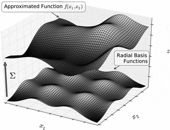
In Fig. 3, the concept of the method is shown graphically for a 2D function. The unknown function
 $\underline{\hat{c}}_{F}(t) = f(\underline{x}(t))$
is approximated with a weighted super-position of radial basis functions
 $a_i(\underline{x}(t))$
(see Equation (7)).
 $$\begin{equation}
\underline{\hat{c}}_F(t) = f(\underline{x}(t)) = g(\underline{x}(t)) + \sum ^{N}_{i=1} \underline{w}_i a_i(\underline{x}(t))
\end{equation}$$
Visualisation of the approximation concept of an unknown function f(x 1, x 2) via a sum of weighted RBF.

Here,
 $g(\underline{x}(t))$
denotes a polynomial, in general constant or linear, submodel in order to cover offsets or linear effects, respectively. In this paper, a constant sub-model
 $g(\underline{x}(t))=const$
is used for all analyses. The determination of the weight matrix
 $\underline{\underline{W}}$
containing the weight vectors
 $\underline{w}_i$
is the aim of the identification process, also called the training or learning process. The target output vector
 $\underline{\hat{c}}_{F}(t)$
contains the POD coefficients of the normalised aerodynamic forces
 $\underline{c}_{F}(t)$
. Thus, the dimension of
 $\underline{\hat{c}}_{F}(t)$
equals the number of output POD modes Mout
.
For the transfer function
 $a_i(\underline{x}(t))$
in Equation (7), any known type of RBF can be used. In this research, the popular Gaussian function
 $a^G_i(\underline{x}(t))$
(see Equation (8)) as well as the inverse quadric (IQ) function
 $a^{IQ}_i(\underline{x}(t))$
(see Equation (9)) are considered as proposed for instance by Kecman(Reference Kecman22) or de Boer et al(Reference de Boer, van der Schoot and Bijl24).
 $$\begin{equation}
a^G_i(\underline{x}(t)) = e^{-\frac{\left(\underline{x}(t)-{\underline{c}_i}\right) \underline{\underline{S}} \left(\underline{x}(t)-{\underline{c}_i}\right)}{r^2_i}} \\
\end{equation}$$
 $$\begin{equation}
a^{IQ}_i(\underline{x}(t)) = \frac{1}{\frac{\left(\underline{x}(t)-{\underline{c}_i}\right) \underline{\underline{S}} \left(\underline{x}(t)-{\underline{c}_i}\right)}{r^2_i} +1}
\end{equation}$$
The vector
 $\underline{c}_i$
denotes the functions centre, and the scalar value ri
is the radius, also known as standard deviation in statistics, of the ith RBF, respectively. In this paper, an RBF is positioned in each known sample point. Moreover, all sample points are projected onto a normed space, i.e. the range of each spatial direction is between 0 and 1. This avoids poor inter-polation results due to different spatial ranges.
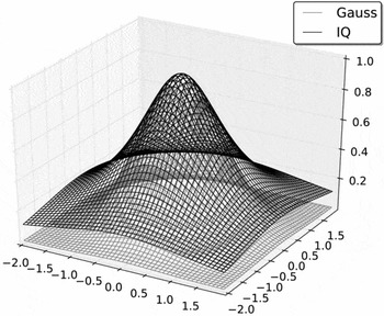
In Fig. 4, the Gaussian RBF is compared with the IQ RBF. Both functions coincide in vicinity to the functions centre
 $\underline{c}_i$
, but for increasing distance aIQ
is significantly larger than aG
.
Comparison of Gaussian and inverse quadric radial basis function.

In order to increase the inter-polation accuracy of the method, the radial function shapes are modified to elliptic shapes. Therefore, a shape matrix
 $\underline{\underline{S}}$
is introduced in Equations (8) and (9), respectively. Kecman(Reference Kecman22) recommends the inverse covariance matrix of all RBF centres as shape matrix
 $\underline{\underline{S}}=\underline{\underline{\Sigma }}^{-1}$
. The investigations for this paper emerged that in combination with the Markov chain model, the inverse covariance matrix
 $\underline{\underline{\Sigma }}^{-1}$
has very large diagonal entries which lead to extreme RBF shapes and hence to instabilities during the identification process.
This is the reason why in this paper an alternate definition of elliptic shapes is used: In order to adapt the functions shapes on the sample distribution, the distances between all RBF centres for each spatial direction is summed up and normalised with the average of entries of the resulting vector (see Equation (10)). The normalisation ensures that the functions shape is manipulated but that the functions influence region is not scaled. The functions influence region is solely scaled by the radius ri .
 $$\begin{equation}
\underline{D} = \frac{\sum ^N_{i=1}\sum ^N_{j=1}(\underline{c}_j-\underline{c}_i)}{avg\left(\sum ^N_{i=1}\sum ^N_{j=1}(\underline{c}_j-\underline{c}_i)\right)}
\end{equation}$$
The shape matrix is then determined by Equation (11). Here,
 $\underline{\underline{I}}^{\dim (\underline{D})}$
denotes the identity matrix with the dimension of
 $\underline{D}$
, and thus
 $\underline{\underline{S}}$
is a diagonal matrix with the normalised distances as diagonal entries
 $diag(\underline{\underline{S}})=\underline{D}$
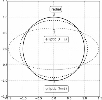
. Additionally, the elliptic shape exponent k is introduced in order to get more extreme elliptic shapes. In application, k is found by performing parametric studies. In Fig. 5, the radial shape is compared with the elliptic shapes (
 $\underline{D}^T=(1.1, 0.9)$
) for k = 1 and k = 4.
 $$\begin{equation}
\underline{\underline{S}} = \underline{\underline{I}}^{\dim (\underline{D})} \text{ } \underline{D}^k
\end{equation}$$
Influence of shape matrix
 $\underline{\underline{S}}$
on the radial shape (
 $\underline{D}^T=(1.1, 0.9)$
).

Another important aspect is the overlapping of the radial basis functions as well as the smoothness of the resulting super-positioned function. Regarding the overlapping of the radial basis functions, an adaptive function radius ri for each RBF is introduced by Lindhorst et al(Reference Lindhorst, Haupt and Horst25,Reference Lindhorst, Haupt and Horst17) (see Equation (12)).
 $$\begin{equation}
r_i = \frac{f_{overlap}}{N} \sum ^N_{j=1}\|{\underline{c}_j}-{\underline{c}_i}\|^2
\end{equation}$$
The overlapping of the functions is controlled with an overlapping factor foverlap scaling the adaptive radius of all functions. The overlapping factor is set to foverlap = 1.0 in this research that ensures a sufficient overlapping of radial basis functions.
For function smoothing, a regularisation parameter λ
s
is defined that is also described by Kecman(Reference Kecman22,Reference Orr23) and Lindhorst et al(Reference Lindhorst, Haupt and Horst17). The parameter λ
s
is called ‘smoothing factor’ in this research. According to Kecman, λ
s
is involved in the determination of the weight matrix
 $\underline{\underline{W}}$
by manipulating the calculation of the pseudo-inverse
 $\underline{\underline{A}}_{inv}$
during the training process (see Equation (13)).
 $$\begin{equation}
\underline{\underline{A}}_{inv} = (\underline{\underline{A}}^T \underline{\underline{A}} +\lambda _s \underline{\underline{I}}^N)^{-1}\underline{\underline{A}}^T
\end{equation}$$
The design matrix
 $\underline{\underline{A}}$
contains the function values of all RBF at the known sample points. With
 $\underline{\underline{A}}_{inv}$
, the weight matrix is determined with Equation (14).
 $$\begin{equation}
\underline{\underline{W}} = \underline{\underline{A}}_{inv} \underline{\underline{T}}
\end{equation}$$
The matrix
 $\underline{\underline{T}}$
denotes the target matrix that contains the target outputs of all known sample points. For λ
s
= 0, the RBF-ANN inter-polates and for λ
s
> 0 the RBF-ANN approximates the given data. An adequate value for λ
s
is found through parametric studies.
3.0 HIRENASD WING MODEL
The HIRENASD wing model is defined and investigated within the DFG (German Research Association)-funded SFB401 project. It is provided through the Aeroelastic Prediction Workshop (AePW) launched on the IFASD 2011(Reference Heeg, Ballmann, Bhatia, Blades, Boucke, Chwalowski, Dietz, Dowell, Florance, Hansen, Mani, Mavriplis, Perry, Ritter, Schuster, Smith, Taylor, Whiting and Wieseman26,Reference Chwalowski, Florance, Heeg, Wieseman and Perry27) . The HIRENASD model is already used by Lindhorst et al(Reference Lindhorst, Haupt and Horst28) for surrogate model investigations at higher angles-of-attack.
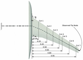
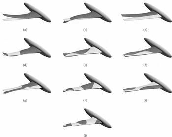
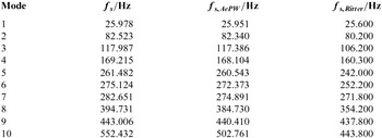
The wing structure is represented by a NASTRAN beam model provided by A. Boucke and C. Wieseman via the AePW homepage(Reference Wieseman and Boucke29). In Fig. 6, the structure model as well as the aerodynamic surface with the investigated cut planes are displayed. The cut plane positions are defined by the normed span-wise coordinate η = y/ymax with ymax = 1.29396m. The displacement of the beams marked tip node is used for tracking the wing motion in Section 4.2. The structure model overhangs the aerodynamic model at the wing tip. In order to preserve the structure dynamic behaviour of the provided beam model, this overhang is not cut off. The mass and stiffness matrices are extracted from the NASTRAN model and used for time integration with the Newmark iteration, which is described by Hughes(Reference Hughes and McCulley30). In Fig. 7, the first ten eigenmodes are shown, which are inter-polated on the aerodynamic grid. According to Table 1, the eigenfrequencies coincide with other references in an acceptable manner. The fuselage is not coupled to the structural model in accordance to Braun(Reference Braun31).
Structural beam model and aerodynamic coupling surface with cut positions for comparison of discrete surface forces(Reference Lindhorst, Haupt and Horst28).

First ten eigenmodes of the structure model inter-polated on the aerodynamic surface.

Comparison of calculated eigenfrequencies of the used beam model with reference values
 ${\bm f}_{\bm{s,AePW}}$
provided on the AePW homepage(Reference Wieseman and Boucke33) and
 ${\bm f}_{\bm{s,Ritter}}$
given by M. Ritter(Reference Ritter34) respectively.

The projection technique used for force as well as displacement inter-polation between the aerodynamic surface and the FEM-beam is implemented following the description of Reimer et al(Reference Reimer, Braun, Wellmer, Behr, Ballmann and Schröder32) as well as Braun et al(Reference Braun31).
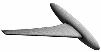
For the aerodynamic analyses, three SOLAR grids(Reference Ritter35,Reference Ritter36,Reference Ritter37) are considered, which are provided by M. Ritter through the AePW homepage. A preliminary comparative study emerge that the medium grid is sufficient for this research. The coupling surface of the medium grid is shown in Fig. 8. It consists of 2,448,805 nodes with 47,657 surface nodes. Consequently, the surrogate model has to predict 142,971 force quantities due to the three force components of each node. Turbulence is modelled by using the Spalart-Allmaras model and assuming fully turbulent flow. The flow conditions of the investigated cases are given in Table 2. The conditions of case 1 are taken from test case 132 given by Chwalowski(Reference Chwalowski, Florance, Heeg, Wieseman and Perry27). In case 2, the free stream temperature is increased by ΔT = 100K with a fixed Mach as well as Reynolds number and the remaining flow parameters are determined via the Sutherland model.
Coupling surface of the used medium SOLAR grid.(Reference Ritter36)

Aerodynamic conditions of the investigated cases

3.1 Training data
The surrogate model is identified from transient forced motion training data. The training set used in this paper consists of three analyses with superimposed excitations of scaled structural mode shapes
 $\underline{u}_s$
of the first ten eigenmodes, which is shown in Equation (15).
 $$\begin{equation}
\underline{u}_{beam} (t) = \sum ^{10}_{s=1} q_s(t) \underline{u}_s \\
\end{equation}$$
 $$\begin{equation}
q_s(t) = q_{s,max} \left(1 - e^{-25t} \right) \sin \left(2 \pi f_s t (1 - 0.1 \sin \left(\frac{2 \pi f_s}{15} t \right) \right)
\end{equation}$$
The generalised coordinate qs of the sth structural eigenmode at time t is determined with Equation (16), which ensures a cumulative growth of the amplitude until q s, max is reached as well as a modulation of excitation frequency of ± 10% of the eigenfrequency. This procedure is already shown in former investigations by Lindhorst et al(Reference Lindhorst, Haupt and Horst17,Reference Lindhorst, Haupt and Horst28) in order to prevent sensitivities of the surrogate model on frequency variations. In Table 3, the generalised coordinates of the three forced motion analyses used for model training are shown. The third and seventh eigenmode (see Figs 7(c) and (g)) leads to problematic deformation in the wing root. According to Ritter(Reference Ritter34), these eigenmodes show less contribution to the aeroelastic deformation in test case 252 at α = 3°. Therefore, it is assumed that the aerodynamic response to the third and seventh eigenmode must not be captured by the surrogate model, and hence it is not included in the training signal.
Generalised coordinates of forced motion training signal

Ritter(Reference Ritter34) used 64 steps per period of the first eigenfrequency that leads to a discrete time step size of ΔtRitter = 1.98 × 10⁻⁴ s. This step size approximately coincide with the time step size of Δt = 0.0002s used in this paper. The training analyses are conducted at case 1 conditions given in Table 2.
3.2 Surrogate model identification
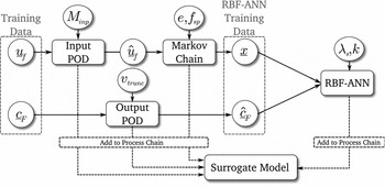
For the model identification process, several parameters have to be defined. These are the number of modes of the input POD base Minp , the number of modes of the output POD base Mout , the time window size e and the sparse factor fsp of the Markov chain model and finally the smoothing factor λ s and the elliptic shape exponent k of the RBF-ANN. The procedure of the surrogate model training process is given in Fig. 9.
Flow chart of the surrogate model identification process.

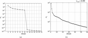
In Fig. 10(a), the first 15 singular values of the input POD base are displayed. Due to the significant decrease of singular values at mode 9, the POD base is reduced to Minp = 8 base vectors. This coincides with the excited eight eigenmodes in the training signal (see Table 3). The singular values of the output POD base are shown in Fig. 10(b). In this case, a truncation criterion of vtrunc = 0.99 is defined, which is a recommended value for the most systems. This criterion leads to Mout = 49 base vectors.
(a) Singular values of the input POD base, (b) Singular values of the output POD base.

The time window size depends on the observed system, namely the system memory. The system memory can be assumed as the time span that a disturbance influences the system response. Investigations showed, that a time window size of a half period of the lowest eigenfrequency is sufficient for the most aeroelastic systems. The lowest eigenfrequency of f 1 = 25.978Hz and the time step size of Δt = 0.0002s lead to a time window size of 100 steps. Additionally, a sparse factor of fsp = 25 is used.
An important aspect is the evaluation of the RBF-ANN accuracy during identification. A widely used concept for accuracy evaluation is the cross-validation method, i.e. several sample points are extracted from the training set that are not used for identification but for error estimation. These points are called cross-validation points in the following. In this study, every second sample point of all known training samples are taken as cross-validation point. This leads to seval = 1500 cross-validation points. In order to evaluate the model accuracy, a quality index Q is introduced, which is shown in Equation (17). Q denotes the mean of the relative error at all cross-validation points.
 $$\begin{equation}
Q = \frac{1}{s_{eval}} \sum ^{s_{eval}}_{i=1} \frac{|| \underline{\hat{c}}_{F,i} - f({\underline{x}}_i) ||}{|| \underline{\hat{c}}_{F,i}||}
\end{equation}$$
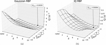
The parameters of the RBF-ANN, namely the choice of the radial basis function, the smoothing factor λ s and the elliptic shape exponent k, are found through parametric studies. In Fig. 11 the value of the quality index Q for different λ s and k is shown. According to the parametric study Q becomes minimal for an RBF-ANN with IQ functions, λ s = 10−5 and k = 9.
Cost function values of the parametric study: (a) Gauss-RBF, (b) IQ-RBF.

In Table 4, the computational effort of the identification process is given. The POD bases are constructed once and then used for each surrogate model in the parametric study.
Computational effort of surrogate model identification

4.0 RESULTS
In this section, the proposed approach is applied within an aero-structural coupling scheme in the time domain. The CFD solver is completely substituted by the reduced order surrogate model and then the ROM-CSM scheme is compared with the CFD-CSM scheme in various aeroelastic analyses. The coupling of the codes is performed by using the ifls coupling environment presented by Haupt et al(Reference Haupt, Niesner, Unger and Horst38). The CFD solver used for reference results is the TAU code(Reference Gerhold, Hannemann and Schwamborn39) of the Deutsches Zentrum für Luft- und Raumfahrt (DLR). The ROM-CSM scheme is compared with the CFD-CSM scheme in static aeroelastic as well as transient aeroelastic analyses.
4.1 Static analysis
In the static analysis the aeroelastic equilibrium state of the coupled model determined with the CFD-CSM scheme is compared with the ROM-CSM scheme. Only the static part of the surrogate model is used for prediction (see Equation (6)). Five fluid-structure iterations (Dirichlet-Neumann iterations) are performed to reach the aeroelastic equilibrium. The first static analysis is conducted at case 1 flow conditions (see Table 2).
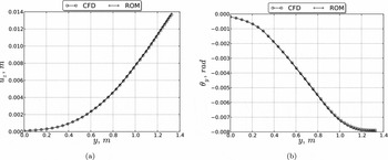
In Fig. 12, the beam deflection
 $\underline{u}_z$
and torsion
 $\underline{\theta }_y$
of the aeroelastic equilibrium is displayed for the CFD-CSM and ROM-CSM analysis. The structural deformation of both analyses coincide in an acceptable manner. The errors of the beam deflection and rotation at the tip node given in Table 5 are smaller than 2% and hence within acceptable bounds.
Beam deformation of static aeroelastic equilibrium at flow conditions of case 1: (a) Displacement in z-direction over y; (b) Rotation around y-axis over y.

Comparison of tip node deflection and rotation in the aeroelastic equilibrium

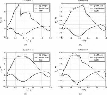
In Fig. 13, the discrete aerodynamic forces of the ROM-CSM analysis are compared with the CFD-CSM analysis in cut sections 4 through 7. In order to indicate the changes of the forces between the un-deformed wing and the aeroelastic equilibrium the forces of the jig shape are also displayed. As shown in the diagrams, the forces of the equilibrium state are predicted sufficiently by the ROM. Larger deviations are visible in cut Section 7 in vicinity to the shock. These deviations can be explained with local non-linear effects in this region due to the shock that are not captured properly by the ROM. However, the influences of structural deformation on the discrete forces are covered with an acceptable accuracy.
Aerodynamic forces in the aeroelastic equilibrium predicted by the ROM and calculated by the CFD as well as CFD calculated forces of the jig shape: (a) cut 4, (b) cut 5, (c) cut 6 and (d) cut 7.

In Table 6, the computational effort of both analyses are given. The given CPU time is the sum of computational time of all used processors. The average time for each ROM prediction is about tpred = 1.35s. The remaining time is needed for other operations such as grid inter-polation.
Computational effort of the static aeroelastic analysis at case 1 conditions

In order to demonstrate the ability of the surrogate model to capture changes of flow conditions at a fixed Mach number, the static analysis is repeated at the conditions of case 2 (see Table 2). For this analysis, the surrogate model is neither modified nor re-identified.
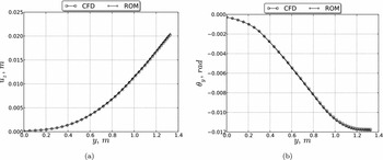
In Fig. 14, the structural deflection and rotation of the aeroelastic equilibrium is shown. The equilibrium state predicted by the ROM coincide fairly with the results of the CFD-CSM analysis. The errors of the beams tip node given in Table 7 are comparable to the errors at case 1 conditions (see Table 5).
Beam deformation of static aeroelastic equilibrium at flow conditions of case 2: (a) Displacement in z-direction over y; (b) Rotation around y-axis over y.

Comparison of tip node deflection and rotation in the aeroelastic equilibrium at case 2

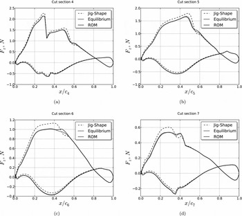
The discrete forces of the aeroelastic equilibrium are shown in Fig. 15 for cut sections 4 through 7. As it can be seen, the ROM predicted forces coincide with the CFD calculated forces in an acceptable manner. Only in cut section 6 are deviations in the shock region noticeable. In contrast to that in cut section 7, the differences in vicinity to the shock are smaller than in case 1 (see Figs 13(d) and 15(d)).
Aerodynamic forces in the aeroelastic equilibrium predicted by the ROM and calculated by the CFD as well as CFD calculated forces of the jig shape at case 2 conditions: (a) cut 4, (b) cut 5, (c) cut 6, (d) cut 7.

However, this demonstrates that in static analysis change of free stream temperature of ΔT = 100K is fairly captured by the ROM.
4.2 Transient analysis
In this investigation, the transient coupled system is observed. An iterative staggered coupling is used with a second-order structural predictor in accordance to Unger et al(Reference Unger, Haupt and Horst40). The initial displacement, velocity and acceleration of the wing is set to zero. Therefore, the system is not in an equilibrium state in the beginning of the analysis and the wing starts a free motion oscillation. The analysis is conducted for 500 time steps with a time step size of Δt = 0.0002s.
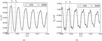
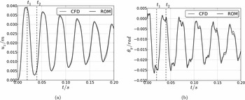
First, the free oscillation of the wing is considered at case 1 flow conditions (see Table 2). In Fig. 16, the tip node displacement u z, Tip and rotation θ y, Tip is displayed over the time. The structural motion of the ROM-CSM analysis coincide in an acceptable manner with the corresponding CFD-CSM analysis.
Results of transient analysis at case 1 conditions: (a) Tip node displacement u z, Tip , (b) Tip node rotation θ y, Tip .

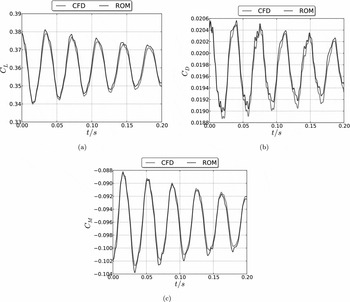
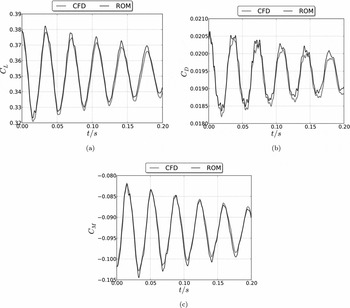
In Fig. 17, the global aerodynamic coefficients are displayed over the time. The global aerodynamic coefficients coincide fairly with the CFD results in the observed time span. In Table 8, the maximal occurring error as well as the average error of the global aerodynamic coefficients are given. The average errors are far smaller than 2%, and hence the prediction accuracy of the surrogate model is within acceptable bounds.
Results of transient analysis at case 1 conditions: (a) Lift coefficient, (b) Drag coefficient, (c) Pitching moment coefficient.

Maximal occurring error
 ${\bm e}_{\bm{max}}$
and average error
 ${\bm e}_{\bm{avg}}$
of the global aerodynamic coefficients
 ${\bm C}_{\bm L}$
,
 ${\bm C}_{\bm D}$
and
 ${\bm C}_{\bm M}$
in the transient analysis at case 1 conditions

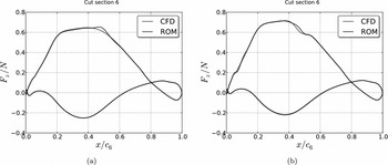
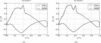
In order to have a closer look into the discrete aerodynamic forces predicted by the surrogate model, in Figs 18 and 19 the predicted forces in cut 6 and 7 (see Fig. 6) are compared with the CFD calculated forces for time t 1 = 0.02s and t 2 = 0.04s. According to Fig. 16, the structural deflection at time t 1 is in the first upper apex, and t 2 is in the first lower apex of u z, Tip . The predicted forces fairly match the CFD calculated forces. Small deviations are noticeable in vicinity to the shock. At time t 2 in cut 7, differences also occur in the entire super-sonic region on the suction side. This can be explained with the representation of the lower apex in the training set.
Comparison of forces in cut section 6: (a) t 1 = 0.02; (b) t 2 = 0.04.

Comparison of forces in cut section 7: (a) t 1; (b) t 2.

After considering the free oscillation of the wing at case 1 conditions, the investigation is repeated with case 2 conditions. In Fig. 20, the tip node displacement as well as rotation is shown. Again, the structural motion of the ROM-CSM analysis fairly coincide with the results of the CFD-CSM analysis.
Results of transient analysis at case 2 conditions: (a) Tip node displacement u z, Tip , (b) Tip node rotation θ y, Tip .

In Fig. 21, the global aerodynamic coefficients are displayed over the time. The prediction accuracy is comparable to the analysis with case 1 conditions. The maximal occurring error as well as the mean error of the aerodynamic coefficients are given in Table 9. Compared to the mean errors at case 1 conditions (see Table 8), the mean errors at case 2 conditions increase slightly. However, the errors are still smaller than 2% and hence within acceptable bounds. This investigation shows, that the surrogate model is able to capture the changes of flow conditions fairly at a fixed Mach and Reynolds number.
Results of transient analysis at case 2 conditions: (a) Lift coefficient, (b) Drag coefficient, (c) Pitching moment coefficient.

Maximal occurring error
 ${\bm e}_{\bm{max}}$
and average error
 ${\bm e}_{\bm{avg}}$
of the global aerodynamic coefficients
 ${\bm C}_{\bm L}$
,
 ${\bm C}_{\bm D}$
and
 ${\bm C}_{\bm M}$
in the transient analysis at case 2 conditions

In Table 10, the computational effort of the ROM-CSM and CFD-CSM analyses in both cases are given. Please note that the given CPU time is the sum of computational effort of all used processors. Again, the average time for each ROM prediction is about tpred = 1.35s. As it can be seen, a significant speed-up of the coupled analysis can be achieved. According to Table 10, the surrogate model reduces the analysis time significantly.
Computational effort of the transient aeroelastic analysis at case 1 conditions

5.0 CONCLUSIONS
In this paper, the transient, non-linear surrogate model approach presented in Lindhorst et al(Reference Lindhorst, Haupt and Horst17) is applied to the HIRENASD wing fuselage configuration that represents a realistic transport aircraft wing. The prediction accuracy of the surrogate model is compared with CFD results in static as well as free motion investigations.
It is shown that the prediction accuracy of the approach is sufficient in all conducted analyses, although the surrogate models are identified from transient data. Due to the use of a RANS solver with the Spalart-Allmaras turbulence model, the surrogate model takes the influence of viscous effects on the aerodynamic forces into account. Moreover, it is demonstrated that limited variations of flow conditions at a fixed Mach number are covered by the surrogate model due to parameter normalisation. Consequently, once the model is identified, it can be applied in an aerostructural coupling scheme and used in various static as well as transient aeroelastic investigations with a fraction of the time compared to the corresponding CFD analyses.
On-going work is the introduction of the Mach number, angle-of-attack as well as Reynolds number as an additional degree of freedom. Future challenges are the use of the surrogate model approach in aeroelastic gust or manoeuvre investigations.
ACKNOWLEDGEMENTS
The authors thank Markus Ritter of DLR for valuable discussions and his support with HIRENASD models and data as well as Marco Gerhardt of TU Braunschweig for his support.