2.1 Elements of the linear-parameter-varying engine model

The model from Fig. 2 consists of the following elements: inlet conditions, input to the system, scheduling variables, system states, system outputs, transformation gains, offset maps and dynamic maps. These are described in the following subsections.

2.1.1 Inlet conditions and the transformation gains

The external operating conditions, i.e. altitude, Mach number and temperature variations, define the conditions of the air at the engine inlet, and have a considerable impact on how the engine behaves. Nevertheless, it is possible to account for the variations in these conditions by using referred corrections [Reference Walsh and Fletcher1]. These corrections are typically performed with coefficients that are function of the inlet temperature and pressure, and depending on which variable is being referred, a different parameter is used. For example, the shaft speed is corrected by the square root of the parameter $\theta $ , while the shaft acceleration is referred by using the parameter $\delta $ . Let us recall here the definition [Reference Walsh and Fletcher1] of these two coefficients:

(1) \begin{align} \delta = \frac{{{P_{inlet}}}}{{{P_{SLS}}}},{\rm{\;\;\;\;\;\;\;\;}}\theta = \frac{{{T_{inlet}}}}{{{T_{SLS}}}}, \end{align}

where the subscript inlet refers to the inlet total conditions of the engine, which are variable in time, and the subscript SLS refers to sea-level-static conditions, which are constant.

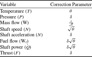
A table with the common engine variables and their respective correction coefficients can be seen in Appendix A. The inlet conditions are therefore defined as in the following equation:

(2) \begin{align} {\phi _{(t)}} = \left[ {\begin{array}{c}{{\delta _{(t)}}}\\{{\theta _{(t)}}}\end{array}} \right]. \end{align}

Using the inlet conditions, the transformation matrices ${S_{{u_{(\phi)}}}} \in {\mathbb{D}^{{n_u}}}$ for the input, ${S_{{\alpha _{(\phi)}}}} \in {\mathbb{D}^{{n_\alpha }}}$ and ${S_{{{\dot \alpha }_{(\phi)}}}} \in {\mathbb{D}^{{n_\alpha }}}$ for the scheduling variable and its derivative, ${S_{{x_{(\phi)}}}} \in {\mathbb{D}^{{n_x}}}$ and ${S_{{{\dot x}_{(\phi)}}}} \in {\mathbb{D}^{{n_x}}}$ for the state and its derivative, and ${S_{{y_{(\phi)}}}} \in {\mathbb{D}^{{n_y}}}$ for the output are defined, containing in their diagonal the correction coefficients corresponding to each signal. For example, if the state of the system consists of a vector with two shaft speeds, the transformation matrix ${S_{{x_{(\phi)}}}}$ would be a square matrix of size two, with the coefficient for the shaft speeds in both its diagonal elements, as per:

(3) \begin{align} {S_{{x_{(\phi)}}}} = \left[ {\begin{array}{c@{\quad}c}{\sqrt \theta } & 0 \\ 0 & {\sqrt \theta }\end{array}} \right]. \end{align}

2.1.2 Input to the system

The signal ${\bar u_{(t)}} \in {\mathbb{R}^{{n_u}}}$ represents all the inputs to the system, i.e. fuel flow, geometry variation, and offtakes. This input is referred to its SLS equivalent ${u_{(t)}} \in {\mathbb{R}^{{n_u}}}$ via left-multiplying it by the inverse of the input correction matrix ${S_{{u_{(\phi)}}}}$ , as per

(4) \begin{align} {u_{(t)}} = S_{{u_{(\phi)}}}^{ - 1}{\bar u_{(t)}}. \end{align}

2.1.3 Scheduling variable

The internal scheduling variable ${\bar \alpha _{(t)}} \in {\mathbb{R}^{{n_\alpha }}}$ is an abstraction of the level of power at which the engine is operating. It can be one, or several, of the variables relevant to the power rating, e.g. fan speed, engine pressure ratio or thrust [Reference Samar and Postlethwaite20], or even a combination of them. In this paper however, we are proposing to use only one scheduling variable, as it has been shown in the literature [Reference Jia, Shi, Li, Han and Xiao15, Reference Mahmood, Griffin, Fleming and Shutler21], as well as our testing in section 4, to be sufficient to represent the changes in engine behaviour.

Inspired by the work in the design of a feedback linearising engine controller using inversion of dynamics [Reference Mahmood, Griffin, Fleming and Shutler21], the scheduling variable will be chosen as a normalised version of the high-pressure shaft speed, in the absence of changes in the geometry or offtakes, i.e. it will be an idealised version of the high-pressure shaft speed, that only takes into account the changes in the fuel flow. The geometry will be assumed to follow its nominal values, as per the performance engineers have prescribed, and with no offtake (or with a constant one).

The derivative of the scheduling variable is calculated in referred coordinates following the expression:

(5) \begin{align} {\dot \alpha _{(t)}} = {J_{(\alpha)}}\big( {{u_{(t)}} - {\mathcal{u}_{(\alpha)}}} \big), \end{align}

where the matrix ${J_{(\alpha)}} \in {\mathbb{R}^{{n_\alpha } \times {n_u}}}$ is the transition matrix that governs the scheduling dynamics at SLS, and ${\mathcal{u}_{(\alpha)}} \in {\mathbb{R}^{{n_u}}}$ is the input offset at the linearisation point.

Before integration, the scheduling variable is returned to the current operating conditions by multiplication with the correction matrix ${S_{{{\dot \alpha }_{(\phi)}}}}$ , and then referred to SLS with the matrix ${S_{{\alpha _{(\phi)}}}}$ , as in the following expressions:

(6) \begin{align} {\dot {\bar \alpha} _{(t)}} = {S_{{{\dot \alpha }_{(\phi)}}}}{\dot \alpha _{(t)}}, \\[-25pt] \notag \end{align}

(7) \begin{align} {\bar \alpha _{(t)}} = {\bar \alpha _{\left( 0 \right)}} + \mathop \smallint \nolimits_0^t {\dot{ \bar \alpha} _{\left( \tau \right)}}{\rm{\;}}d\tau , \\[-25pt] \notag \end{align}

(8) \begin{align} {\alpha _{(t)}} = S_{{\alpha _{(\phi)}}}^{ - 1}{\bar \alpha _{(t)}}. \\[-25pt] \notag \end{align}

2.1.4 System state

The variables that capture the dynamic behaviour of the engine are represented by the state vector ${\bar x_{(t)}} \in {\mathbb{R}^{{n_x}}}$ , which in this paper are considered to be the shaft speeds, as it is common practice when modelling gas turbine engines [Reference Jaw and Mattingly10, Reference Chapman and Litt19]. The state derivative is calculated in referred coordinates following the expression:

(9) \begin{align} {\dot x_{(t)}} = {A_{(\alpha)}}\left( {{x_{(t)}} - {\mathcal{x}_{(\alpha)}}} \right) + {B_{(\alpha)}}\left( {{u_{(t)}} - {\mathcal{u}_{(\alpha)}}} \right), \end{align}

where the matrices ${A_{(\alpha)}} \in {\mathbb{R}^{{n_x} \times {n_x}}}$ and ${B_{(\alpha)}} \in {\mathbb{R}^{{n_x} \times {n_u}}}$ are respectively the state transition matrix and the input matrix, and ${\mathcal{x}_{(\alpha)}} \in {\mathbb{R}^{{n_x}}}$ is the state offset, all evaluated at the linearisation point given by the value of $\alpha $ at time $t$ .

As with the scheduling variable, the state is returned to the current operating conditions before integration, by multiplication with the correction matrix ${S_{{{\dot x}_{(\phi)}}}}$ , and then referred back to SLS with the matrix ${S_{x(\phi)}}$ , as in:

(10) \begin{align} {\dot {\bar x}_{(t)}} = {S_{{{\dot x}_{(\phi)}}}}{\dot x_{(t)}}, \\[-25pt] \notag \end{align}

(11) \begin{align} {x_{(t)}} = S_{x(\phi)}^{ - 1}{\bar x_{(t)}}. \end{align}

2.1.5 System output

The variables of interest, i.e. those variables required in the application that will use this model, are the system outputs in ${\bar y_{(t)}} \in {\mathbb{R}^{{n_y}}}$ . These may be a set of pressures, temperatures, mass flows, shaft speeds or even thrust.

The output is calculated in referred coordinates as per the expression:

(12) \begin{align} {y_{(t)}} = {\mathcal{y}_{(\alpha)}} + {C_{(\alpha)}}\left( {{x_{(t)}} - {\mathcal{x}_{(\alpha)}}} \right) + {D_{(\alpha)}}\left( {{u_{(t)}} - {\mathcal{u}_{(\alpha)}}} \right),\end{align}

where the matrices ${C_{(\alpha)}} \in {\mathbb{R}^{{n_y} \times {n_x}}}$ and ${D_{(\alpha)}} \in {\mathbb{R}^{{n_y} \times {n_u}}}$ are respectively the output matrix and the feedthrough matrix, and ${\mathcal{y}_{(\alpha)}} \in {\mathbb{R}^{{n_y}}}$ is the output offset, all evaluated at the linearisation point given by the value of $\alpha $ at time $t$ .

The output is referred back to the current operating conditions by multiplication with the correction matrix ${S_{{y_{(\phi)}}}}$ , as in:

(13) \begin{align} {\bar y _{(t)}} = {S_{{y_{(\phi)}}}}{y_{(t)}}. \\[-25pt] \notag \end{align}

2.2 The structure of the dynamics maps

When identifying a system using an LPV representation, the approach to be considered could consist in interpolating between different models running in parallel, with the computational burden that running a large number of models in parallel would entail, or interpolating the coefficients used in one single model. The latter takes typically the form of a piece-wise representation of the system matrices, simpler to identify using local experiments, in contrast to more complex forms, like the one chosen here: the polynomial representation.

2.2.1 Piece-wise representation

The standard representation of LPV matrices, for example in the case of ${A_{(\alpha)}}$ , would follow Equation (14), where the weights ${\mu _{{j_{(\alpha)}}}} \in {\mathbb{R}^1}$ are the interpolation coefficients.

(14) \begin{align} {A_{(\alpha)}} = \mathop \sum \limits_{j = 1}^N {\mu _{{j_{(\alpha)}}}}{A_j}. \end{align}

Each matrix ${A_j}$ is typically obtained experimentally at each operating point [Reference Zhang and Ljung17], in isolation from the rest of operating points. This may lead to artificial abrupt changes in the dynamics, making the matrices non-differentiable with respect to the scheduling variable.

2.2.2 Polynomial representation

Constructing the dynamic matrices as in Equation (14) is only possible if the state-space linearisation points are coherent, i.e. if the states have the same meaning at the different linearisation points. This is not necessarily the case when the models are identified from data, at different operating conditions, using black-box identification tools [Reference Zhang and Ljung17].

To address these challenges, we are proposing to use prior knowledge of the structure of the system, fixing the states to known mechanical variables: the shaft speeds of the engine. This provides coherency and interpretability of the models.

Furthermore, in order to preserve the smoothness of the true functions, we are aiming at representing the system dynamic matrices using m-order polynomial functions, as in:

(15) \begin{align} {A_{(\alpha)}} = {A_0} + \alpha {A_1} + {\alpha ^2}{A_2} + \ldots + {\alpha ^m}{A_m},{\rm{\;\;\;\;\;\;\;\;}}{A_{(\alpha)}} = \mathop \sum \limits_{j = 0}^m {\alpha ^j}{A_j}, \end{align}

where the matrices ${A_j}$ have the same dimensions of ${A_{(\alpha)}}$ , and the scheduling variable is a scalar $\alpha \in {\mathbb{R}^1}$ .

3.1 Identification experiments

Two sets of experiments are needed in order to identify the engine as proposed here, both executed at SLS:

• • Staircase in fuel flow. The experiment consists in setting all disturbances to their nominal constant value, all the geometry to their design schedule, and introduce a staircase signal in fuel flow to the engine, leaving enough simulation time between steps to allow the system to settle. From this experiment, the offset maps and the scheduling dynamics will be identified. To design the steps magnitude, the fuel flow range is discretised to $n$ operating points, so each step moves the fuel flow from one operating point to the next.

• • Random perturbations at each operating point. A series of experiments will first take the engine to each operating point and then introduce a random sequence of perturbation to all the inputs, to guarantee sufficient excitation [Reference Bamieh and Giarré16]. The matrices defining the state dynamics and the output equation will be identified from these ${n_e}$ experiments.

The number of operating points should be as low as possible to keep the amount of data to a minimum, but high enough to accurately capture the changes in all system variables throughout the power range.

3.2 Static maps and the scheduling variable

The static maps are obtained as the values of all the variables involved, i.e. inputs, states and outputs, when the system is at rest. The data from the first experiment are used here.

The values of the scheduling variable are taken here as the values of the high-pressure shaft speedFootnote ¹ , normalised by its maximum value, i.e. the array of values of the scheduling variable is defined by:

(16) \begin{align} {\alpha _{ss}} = N{H_{ss}}{\rm{\;\;}}{\left( {NH_{ss}^{\, max}} \right)^{ - 1}}. \end{align}

where $NH_{ss} \in \mathbb{R}_ + ^{n_{ss}}$ is an array with the static values of the high-pressure shaft speed at each operating point, and $NH_{ss}^{max}$ $ \in \mathbb{R}_ + ^1$ is the maximum value of that array.

Using this vector, and the data from each of the variables being modelled, the static maps are built as interpolation functions. By way of example, Equation (17) shows the static map definition corresponding to the first input, using linear interpolation between data points.

(17) \begin{align} {\mathcal{u}_1}:{\rm{\;}}{\mathcal{u}_1}_{(\alpha)} = \frac{{\left( {{\alpha _{ss,j}} - \alpha } \right){{\rm{W}}_{\rm{f}}}_{ss,j - 1} + \left( {\alpha - {\alpha _{ss,j - 1}}} \right){{\rm{W}}_{\rm{f}}}_{ss,j}}}{{{\alpha _{ss,j}} - {\alpha _{ss,j - 1}}}}{\rm{\;\;}};{\rm{\;\;}}{\alpha _{ss,j - 1}} \le \alpha \le {\alpha _{ss,j}},{\rm{\;\;}}\forall j = \left[ {2{\rm{\;}} \ldots {\rm{\;}}n_{ss}} \right], \end{align}

where ${\mathcal{u}_1}$ is the first input, chosen as the fuel flow ( ${{\rm{W}}_{\rm{f}}}$ ), and the symbol ${{\rm{W}}_{\rm{f}}}_{ss,j}$ refers to the value of the fuel flow in steady-state, in the data point $j$ .

3.3 Dynamics of the scheduling variable

In order to model how the scheduling variable changes in time as a function of the input, the entire dataset from the first experiment will be used, including the parts consisting of system dynamics.

Even though the dynamics are defined in continuous time in Equation (5), the data is assumed to be recorded in discrete-time, at a constant sampling period ${{\rm{\Delta }}_t}$ . Discretisation of Equation (5) by forward Euler [Reference Biswas, Chatterjee, Mukherjee and Pal22] for sufficiently small ${{\rm{\Delta }}_t}$ yields:

(18) \begin{align} {\dot \alpha _{(t)}} = \mathop {{\rm{lim}}}\limits_{{{\rm{\Delta }}_t} \to {\rm{\;}}0} \frac{{{\alpha _{\left( {t + {{\rm{\Delta }}_t}} \right)}} - {\alpha _{(t)}}}}{{{{\rm{\Delta }}_t}}}, \end{align}

(19) \begin{align} {\alpha _{\left( {t + {{\rm{\Delta }}_t}} \right)}} \approx {\alpha _{(t)}} + {{\rm{\Delta }}_t}{\rm{\;}}{J_{(\alpha)}}{\rm{\;}}\left( {{u_{(t)}} - {\mathcal{u}_{(\alpha)}}} \right). \\[5pt] \notag\end{align}

Renaming the time variable by its discrete sample equivalent, and rearranging Equation (19) leads to:

(20) \begin{align} {\alpha _{\left( {k + 1} \right)}} - {\alpha _{\left( k \right)}} = \left[ {{\rm{\;}}{J_0}{\rm{\;\;}}{J_1}{\rm{\;\;}}{J_2}{\rm{\;}} \cdots {\rm{\;}}{J_{{m_J}}}{\rm{\;}}} \right]\left( {{\rm{\;\;}}\left[ {\begin{array}{c}1\\{\alpha_{\left( k \right)}}\\[3pt]{\alpha _{\left( k \right)}^2}\\[3pt] \vdots \\[3pt] {\alpha _{\left( k \right)}^{{m_J}}}\end{array}} \right] \otimes \left[ {{\rm{\;}}1{\rm{\;}}0{\rm{\;}} \cdots {\rm{\;}}0{\rm{\;}}} \right]{\rm{\;\;}}} \right)\left( {{u_{\left( k \right)}} - {\mathcal{u}_{\left( {\alpha ,k} \right)}}} \right){{\rm{\Delta }}_t}, \end{align}

where ${m_J}$ is the order of the polynomial, the variables ${J_j} \in {\mathbb{R}^1};\forall j \in \left[ {0 \ldots {m_J}} \right]$ , are the coefficients of the polynomial representation of ${J_{(\alpha)}}$ , and the matrix $\left[ {{\rm{\;}}1{\rm{\;}}0{\rm{\;}} \cdots {\rm{\;}}0{\rm{\;}}} \right]$ is used to select only the first input among the signals in ${u_{\left( k \right)}}$ . A more compact representation of Equation (20) follows:

(21) \begin{align} {\tilde \alpha _{\left( k \right)}} = \skew4\bar J {\rm{\;}}\left( {{\rm{\;}}p_{\left( {\alpha ,k} \right)}^{{m_J}} \quad \otimes \quad \left[ {{\rm{\;}}1{\rm{\;}}0{\rm{\;}} \cdots {\rm{\;}}0{\rm{\;}}} \right]{\rm{\;}}} \right){\rm{\;\;}}{\tilde u_{\left( {\alpha ,k} \right)}}{\rm{\;\;}}{{\rm{\Delta }}_t},{\rm{\;\;\;\;\;\;\;\;}}{\tilde \alpha _{\left( k \right)}} = \skew4\bar J {\rm{\;\;}}{v_{\left( {\alpha ,k} \right)}},\end{align}

where $\skew4\bar J \in {\mathbb{R}^{1 \times \left( {{m_J} + 1} \right)}}$ is the matrix containing the constant coefficients to be identified, $p_{\left( {\alpha ,k} \right)}^{{m_J}} = {[{\rm{\;}}1{\rm{\;\;}}{\alpha _{\left( k \right)}} \cdots \alpha _{\left( k \right)}^{{m_J}}{\rm{\;}}]^T}$ is the array containing the monomials of the polynomial representation, ${\tilde \alpha _{\left( k \right)}}$ is the difference between the values of the scheduling variable at the current and the next samples, ${\tilde u_{\left( {\alpha ,k} \right)}}$ is the difference from the input to the offset as a function of the scheduling variable in the current sample, and ${v_{\left( {\alpha ,k} \right)}}$ is an auxiliary variable that captures the multiplication of the polynomial with the input difference and the sampling period.

The equation is now ready for least-squares identification [Reference Söderström23], by grouping the data from the experiment in array form as per:

(22) \begin{align} \left[ {{\rm{\;}}{{\tilde \alpha }_{\left( 1 \right)}}{\rm{\;\;}}{{\tilde \alpha }_{\left( 2 \right)}}{\rm{\;}} \cdots {\rm{\;}}{{\tilde \alpha }_{\left( {l - 1} \right)}}{\rm{\;}}} \right] = {\bar{J} ^{\rm{*}}}\left[ {{\rm{\;}}{v_{\left( 1 \right)}}{\rm{\;\;}}{v_{\left( 2 \right)}}{\rm{\;}} \cdots {\rm{\;}}{v_{\left( {l - 1} \right)}}{\rm{\;}}} \right],{\rm{\;\;\;\;\Lambda }} = {\skew4\bar J ^{\rm{*}}}V, \end{align}

where $l$ is the number of data points. The solution to the least-squares problem isFootnote ² $\skew4\bar J = {\rm{\Lambda }}{V^T}{\left( {V{V^T}} \right)^{ - 1}}$ . The proof can be found in Appendix B.1.

3.4 Dynamics of the system state

In order to identify the matrices ${A_{(\alpha)}}$ and ${B_{(\alpha)}}$ from the state equation defined by Equation (9), the second set of experiments is used, containing random excitations of the inputs at different operating points.

First, the behaviour of the scheduling variable during each of the experiments has to be obtained. The scheduling variable is not readily available from the data of these experiments because it is a construct that represents the behaviour of the high-pressure shaft when the system is excited exclusively by the fuel flow. Instead, the scheduling variable will be calculated by iterating Equation (19), i.e., iterating the expression:

(23) \begin{align} {\alpha _{\left( {t + {{\rm{\Delta }}_t},i} \right)}} = {\alpha _{\left( {t,i} \right)}} + {{\rm{\Delta }}_t}{\rm{\;}}{J_{\left( {\alpha ,i} \right)}}{\rm{\;}}\left( {{u_{\left( {t,i} \right)}} - {\mathcal{u}_{\left( {\alpha ,i} \right)}}} \right). \end{align}

The initial value for this calculation, i.e. ${\alpha _{\left( {0,i} \right)}}$ , will be taken as equal to the initial value of the high-pressure shaft speed in each experiment, before any changes are introduced to the inputs, and normalised by the same factor that was used in Equation (16), i.e. the scheduling variable for each experiment $i$ starts at:

(24) \begin{align} {\alpha _{\left( {t = 0,i} \right)}} = N{H_{\left( {t = 0,i} \right)}}{\rm{\;}}{\left( {NH_{ss}^{max}} \right)^{ - 1}}, \end{align}

Once the sequence of values of the scheduling variables is built for each experiment using Equation (23), and following the same discretisation approach for the state transition defined in Equation (9), the state dynamics of each experiment $i$ can be formulated as:

(25) \begin{align} {x_{\left( {t + {{\rm{\Delta }}_t},i} \right)}} \approx {x_{\left( {t,i} \right)}} + {{\rm{\Delta }}_t}{\rm{\;}}{A_{\left( {\alpha ,i} \right)}}{\rm{\;}}\left( {{x_{\left( {t,i} \right)}} - {\mathcal{x}_{\left( {\alpha ,i} \right)}}} \right) + {{\rm{\Delta }}_t}{\rm{\;}}{B_{\left( {\alpha ,i} \right)}}{\rm{\;}}\left( {{u_{\left( {t,i} \right)}} - {\mathcal{u}_{\left( {\alpha ,i} \right)}}} \right). \end{align}

The state-transition equation can now be formulated in discrete-time explicitly, with the coefficients and monomials, as per:

\begin{align*} {x_{\left( {k + 1,i} \right)}} - {x_{\left( {k,i} \right)}} = \left[ {{\rm{\;}}{A_0}{\rm{\;\;}}{A_1}{\rm{\;\;}}{A_2}{\rm{\;}} \cdots {\rm{\;}}{A_{{m_A}}}{\rm{\;}}} \right]\left( {{\rm{\;\;}}\left[ {\begin{array}{c}1\\[3pt]{{\alpha _{\left( {k,i} \right)}}}\\[3pt]{\alpha _{\left( {k,i} \right)}^2}\\[3pt] \vdots \\ {_{\left( {k,i} \right)}^{{m_A}}}\end{array}} \right] \otimes {I_{{n_x}}}{\rm{\;\;}}} \right)\left( {{x_{\left( {k,i} \right)}} - {\mathcal{x}_{\left( {\alpha ,k,i} \right)}}} \right){{\rm{\Delta }}_t}{\rm{\;}} + \end{align*}

(26) \begin{align} \left[ {{\rm{\;}}{B_0}{\rm{\;\;}}{B_1}{\rm{\;\;}}{B_2}{\rm{\;}} \cdots {\rm{\;}}{B_{{m_B}}}{\rm{\;}}} \right]\left( {{\rm{\;\;}}\left[ {\begin{array}{c}1\\{{\alpha _{\left( {k,i} \right)}}}\\{\alpha _{\left( {k,i} \right)}^2}\\ \vdots \\{\alpha _{\left( {k,i} \right)}^{{m_B}}}\end{array}} \right] \otimes {I_{{n_u}}}{\rm{\;\;}}} \right)\left( {{u_{\left( {k,i} \right)}} - {\mathcal{u}_{\left( {\alpha ,k,i} \right)}}} \right){{\rm{\Delta }}_t}, \end{align}

where $k$ represents the discrete time step, the variables ${A_j} \in {\mathbb{R}^{{n_x} \times {n_x}}},{\rm{\;}}\forall j \in \left[ {0,{m_A}} \right]$ , and ${B_j} \in {\mathbb{R}^{{n_x} \times {n_u}}},$ $\forall j \in \left[ {0,{m_B}} \right]$ , are the constant coefficients of the polynomial representations of the matrices ${A_{(\alpha)}}$ and ${B_{(\alpha)}}$ , and ${m_A}$ and ${m_B}$ are the order of the polynomials used to model the state transition dynamicsFootnote ³ . A more compact representation of Equation (26) follows:

(27) \begin{align} {\xi _{\left( {k,i} \right)}} = \bar A \left( {{\rm{\;}}p_{\left( {\alpha ,k,i} \right)}^{{m_A}} \otimes {I_{{n_x}}}{\rm{\;}}} \right){\rm{\;}}{\tilde x_{\left( {\alpha ,k,i} \right)}}{\rm{\;}}{{\rm{\Delta }}_t} + \bar B {\rm{\;}}\left( {{\rm{\;}}p_{\left( {\alpha ,k,i} \right)}^{{m_B}} \otimes {I_{{n_u}}}{\rm{\;}}} \right){\rm{\;}}{\tilde u_{\left( {\alpha ,k,i} \right)}}{\rm{\;}}{{\rm{\Delta }}_t},{\rm{\;\;\;\;\;\;\;\;}}{\xi _{\left( {k,i} \right)}} = {{\rm{\Phi }}^{\rm{*}}}{\rm{\;}}{\eta _{\left( {k,i} \right)}} \end{align}

where ${{\rm{\Phi }}^{\rm{*}}} = \left[ {{\rm{\;}}\bar A {\rm{\;\;}}\bar B {\rm{\;}}} \right]$ is the matrix with the coefficients to be identified, $p_{\left( {\alpha ,k,i} \right)}^m = {[{\rm{\;}}1{\rm{\;\;}}{\alpha _{\left( {k,i} \right)}} \cdots \alpha _{\left( {k,i} \right)}^m{\rm{\;}}]^T}$ is the array containing the monomials up to order $m$ , ${\xi _{\left( {k,i} \right)}}$ is the difference between the values of the state at the current and the next samples, ${\tilde x_{\left( {\alpha ,k,i} \right)}}$ is the difference from the state to the offset, ${\tilde u_{\left( {\alpha ,k} \right)}}$ is the difference from the input to the offset, and ${\eta _{\left( {k,i} \right)}}$ is an auxiliary variable defined by Equation (28). All in the current sample $k$ during experiment $i$ .

(28) \begin{align} {\eta _{\left( {k,i} \right)}} = \left[ {{\rm{\;}}\begin{array}{c}{\left( {{\rm{\;}}p_{\left( {\alpha ,k,i} \right)}^{{m_A}} \otimes {I_{{n_x}}}{\rm{\;}}} \right){\rm{\;}}{{\tilde x}_{\left( {\alpha ,k,i} \right)}}}\\{\left( {{\rm{\;}}p_{\left( {\alpha ,k,i} \right)}^{{m_B}} \otimes {I_{{n_u}}}{\rm{\;}}} \right){\rm{\;}}{{\tilde u}_{\left( {\alpha ,k,i} \right)}}}\end{array}{\rm{\;}}} \right]{\rm{\;}}{{\rm{\Delta }}_t}. \end{align}

The equation can now be defined in array form, following the same approach than in Equation (22), which yields:

(29) \begin{align} \left[ {{\rm{\;}}{\xi _{\left( {1,i} \right)}}{\rm{\;}}{{\rm{\;}}\xi_{\left( {2,i} \right)}}{\rm{\;}} \cdots {\rm{\;}}{\xi _{\left( {{l_i} - 1,i} \right)}}{\rm{\;}}} \right] = {{\rm{\Phi }}^{\rm{*}}}\left[ {{\rm{\;}}{\eta _{\left( {1,i} \right)}}{\rm{\;\;}}{\eta _{\left( {2,i} \right)}}{\rm{\;}} \cdots {\rm{\;}}{\eta _{\left( {{l_i} - 1,i} \right)}}{\rm{\;}}} \right],{\rm{\;\;\;\;}}{F_{\left( i \right)}} = {{\rm{\Phi }}^{\rm{*}}}{\rm{\;}}{H_{\left( i \right)}}, \end{align}

where ${l_i}$ is the number of samples available from experiment $i$ , and new matrices ${F_{\left( i \right)}} \in {\mathbb{R}^{{n_x} \times \left( {{l_i} - 1} \right)}}$ and ${H_{\left( i \right)}} \in {\mathbb{R}^{\left( {{n_x}\left( {{m_A} + 1} \right) + {n_u}\left( {{m_B} + 1} \right)} \right) \times \left( {{l_i} - 1} \right)}}$ contain all the data from each experiment $i$ .

We are now ready to formally introduce the main result of this paper:

Lemma 1. The solution $\left( {{\rm{\Phi }},P} \right)$ to the optimisation problem posed in Equation (30) provides the best fit to the system dynamics in the least squares sense, while ensuring the stability of the system, when using polynomials of orders ${m_J}$ , ${m_A}$ and ${m_B}$ .

(30a) \begin{align} \mathop {{\rm{min}}}\limits_{{\rm{\Phi }},P}\quad \frac{1}{{2{\rm{\;}}\left( {\mathop \sum \nolimits_{i = 1}^{{n_e}} \left( {{l_i} - 1} \right)} \right)}}tr\left( {\mathop \sum \limits_{i = 1}^{{n_e}} W_\xi ^{ - 1}\left( {{F_{\left( i \right)}} - {\rm{\Phi }}{H_{\left( i \right)}}} \right){{\left( {{F_{\left( i \right)}} - {\rm{\Phi }}{H_{\left( i \right)}}} \right)}^T}W_\xi ^{ - 1}} \right), \end{align}

(30b) \begin{align} {\rm{s}}{\rm{.t}}{\rm{.}}\quad\;\;\;{({\rm{\Phi }}{M_j})^T}P + P\left( {{\rm{\Phi }}{M_j}} \right) \prec 0;{\rm{\;\;\;\;}}\forall j \in \left[ {1 \ldots {n_{ss}}} \right],{\rm{\;}} \end{align}

(30c) \begin{align} P \succ 0, \end{align}

where ${n_e}$ is the number of experiments, ${n_{ss}}$ is the number of points in the static maps obtained in section 3.2, $P \in \mathbb{S}_{ + + }^{{n_x}}$ is the Lyapunov variable, the matrix ${W_\xi } \in {\mathbb{D}^{{n_x}}}$ contains that maximum values found in the data for each component of the vector $\xi $ in its diagonal, and the matrices ${M_j}$ are defined using the values of the scheduling variable at each point $j$ from the static maps, i.e. ${\alpha _{ss,j}}$ , as per:

(31) \begin{align} {M_j} = \left[ {{\rm{\;}}\begin{array}{c}{{\rm{\;}}p_{\left( {{\alpha _{ss,j}}} \right)}^{{m_A}} \otimes {I_{{n_x}}}}\\{{0_{{n_u}\left( {n + 1} \right) \times {n_x}}}}\end{array}{\rm{\;}}} \right]. \end{align}

The proof is straightforward, and is discussed here briefly:

Conversely, the optimisation problem defined in Equation (30) is not implementable as is, and therefore, in order to solve the problem in practice, we will solve an alternative optimisation. We introduce here the following:

(32a) \begin{align} \mathop {{\rm{min}}}\limits_{{\rm{\Phi }},Q,P,Y,Z}\quad \frac{1}{{2{\rm{\;}}\left( {\mathop \sum \nolimits_{i = 1}^{{n_e}} \left( {{l_i} - 1} \right)} \right)}}tr\left( Q \right), \\[-10pt] \notag \end{align}

(32b) \begin{align} \!\!\!\!\!{\rm{s}}{\rm{.t}}{\rm{.}}\quad \;\;\;\;\left[ {\begin{array}{c@{\quad}c}{\skew4\bar F {{\skew4\bar F }^T} - \skew4\bar F {{\skew4\bar H }^T}{{\rm{\Phi }}^T} - {\rm{\Phi }}\skew4\bar H {{\skew4\bar F }^T} - {W_\xi }Q{W_\xi }} & {{\rm{\Phi }}\skew4\bar H {{\skew4\bar H }^T}} \\[5pt]{\skew4\bar H {{\skew4\bar H }^T}{\rm{\Phi }}} & { - \skew4\bar H {{\skew4\bar H }^T}}\end{array}} \right] &\prec 0{\rm{\;,}} \\[-10pt] \notag\end{align}

(32c) \begin{align} \left[ {\begin{array}{c@{\quad}c}{PY + {Y^T}P} & {{{\left( {{\rm{\Phi }}{M_j}} \right)}^T} + PZ - {Y^T}}\\[5pt ]{\left( {{\rm{\Phi }}{M_j}} \right) + {Z^T}P - Y} & { - Z - {Z^T}}\end{array}} \right] &\prec 0;{\rm{\;\;\;\;}}\forall j \in \left[ {1,{n_{ss}}} \right], \\[-10pt] \notag\end{align}

(32d) \begin{align} P &\succ 0, \\[8pt] \nonumber\end{align}

where $\skew4\bar F = \left[ {{\rm{\;\;}}{F_{\left( 1 \right)}}{\rm{\;}} \cdots {\rm{\;}}{F_{\left( {{n_e}} \right)}}{\rm{\;\;}}} \right]$ and $\skew4\bar H = \left[ {{\rm{\;\;}}{H_{\left( 1 \right)}}{\rm{\;}} \cdots {\rm{\;}}{H_{\left( {{n_e}} \right)}}{\rm{\;\;}}} \right]$ are augmented matrices containing the data from all the experiments. The proof follows from application of the procedure described in Appendix B.4.

3.5 Output equation

The final step consists in the identification of the coefficients to build the polynomial matrices ${C_{(\alpha)}}$ and ${D_{(\alpha)}}$ from Equation (12). The process in this case is simpler than the state transition equation as there are no dynamics involved, and hence, only the multi-experiment nature is to be considered. The data from the same set of experiments as in the previous section are used here.

Once the sequence of values of the scheduling parameter is obtained for each experiment, as described by Equation (23), and following the same manipulation that was performed from Equation (25) to Equation (27), but for the output equation, the following expression is reached:

(33) \begin{align} {\tilde y_{\left( {k,i} \right)}} = \bar C \left( {p_{\left( {p,k,i} \right)}^{{m_C}} \otimes {I_{{n_x}}}} \right){\tilde x_{\left( {k,i} \right)}} + \bar D \left( {p_{\left( {p,k,i} \right)}^{{m_D}} \otimes {I_{{n_u}}}} \right){\tilde u_{\left( {k,i} \right)}},{\rm{\;\;\;\;\;\;\;\;}}{\tilde y_{\left( {k,i} \right)}} = {{\rm{\Omega }}^{\rm{*}}}{\rm{\;}}{\gamma _{\left( {k,i} \right)}} \end{align}

where ${\tilde y_{\left( {k,i} \right)}} = {y_{\left( {k,i} \right)}} - {\mathcal{y} _{\left( {k,i} \right)}}$ is the difference from each output to the corresponding offset, ${{\rm{\Omega }}^{\rm{*}}} = \left[ {{\rm{\;\;}}\bar C {\rm{\;\;}}\bar D {\rm{\;\;}}} \right]$ is the matrix to be identified, with $\bar C = \left[ {{\rm{\;\;}}{C_1}{\rm{\;}} \cdots {\rm{\;}}{C_{{m_C}}}{\rm{\;\;}}} \right]$ and $\bar D = \left[ {{\rm{\;\;}}{D_1}{\rm{\;}} \cdots {\rm{\;}}{D_{{m_D}}}{\rm{\;\;}}} \right]$ containing all the coefficients, while the monomial arrays $p_{\left( {p,k,i} \right)}^{{m_C}}$ and $p_{\left( {p,k,i} \right)}^{{m_D}}$ follow the same structure than the monomials in Equation (27), but with the orders ${m_C}$ and ${m_D}$ . These are grouped together with the state and input deviations in a new variable ${\gamma _{\left( {k,i} \right)}}$ , defined as:

(34) \begin{align} {\gamma _{\left( {k,i} \right)}} = \left[ {{\rm{\;}}\begin{array}{c}{\left( {{\rm{\;}}p_{\left( {\alpha ,k,i} \right)}^{{m_C}} \otimes {I_{{n_x}}}{\rm{\;}}} \right){\rm{\;}}{{\tilde x}_{\left( {\alpha ,k,i} \right)}}}\\[4pt]{\left( {{\rm{\;}}p_{\left( {\alpha ,k,i} \right)}^{{m_D}} \otimes {I_{{n_u}}}{\rm{\;}}} \right){\rm{\;}}{{\tilde u}_{\left( {\alpha ,k,i} \right)}}}\end{array}{\rm{\;}}} \right]. \end{align}

Following the same approach as in Equation (29), the following array form is reached:

(35) \begin{align} \left[ {{\rm{\;}}{{\tilde y}_{\left( {1,i} \right)}}{\rm{\;\;}}{{\tilde y}_{\left( {2,i} \right)}}{\rm{\;}} \cdots {\rm{\;}}{{\tilde y}_{\left( {{l_i},i} \right)}}{\rm{\;}}} \right] = {{\rm{\Omega }}^{\rm{*}}}\left[ {{\rm{\;}}{\gamma _{\left( {1,i} \right)}}{\rm{\;\;}}{\gamma _{\left( {2,i} \right)}}{\rm{\;}} \cdots {\rm{\;}}{\gamma _{\left( {{l_i},i} \right)}}{\rm{\;}}} \right],{\rm{\;\;\;\;}}{E_{\left( i \right)}} = {{\rm{\Omega }}^{\rm{*}}}{\rm{\;}}{G_{\left( i \right)}}, \end{align}

where, in contrast to the state equation, the full set of data points ${l_i}$ of each experiment can be used, since it is a static equation, and the new matrices ${E_{\left( i \right)}} \in {\mathbb{R}^{{n_y} \times {l_i}}}$ and ${G_{\left( i \right)}} \in {\mathbb{R}^{\left( {{n_x}\left( {{m_C} + 1} \right) + {n_u}\left( {{m_D} + 1} \right)} \right) \times {l_i}}}$ gather all the data from each experiment.

The identification problem in this case can be posed as the following unconstrained multi-experiment least-squares optimisation:

(36) \begin{align} \mathop {{\rm{min}}}\limits_{\rm{\Omega }} \frac{1}{{2{\rm{\;}}\left( {\mathop \sum \nolimits_{i = 1}^{{n_e}} {l_i}} \right)}}\mathop \sum \limits_{i = 1}^{{n_e}} tr\left( {W_{\tilde y}^{ - 1}\left( {{E_{\left( i \right)}} - {\rm{\Omega }}{G_{\left( i \right)}}} \right){{\left( {{E_{\left( i \right)}} - {\rm{\Omega }}{G_{\left( i \right)}}} \right)}^T}W_{\tilde y}^{ - 1}} \right). \end{align}

where the matrix ${W_{\tilde y}} \in {\mathbb{D}^{{n_y}}}$ contains, in its diagonal, the maximum values found in the data of the array $\tilde y$ .

The solution to this problem is given by the following expression, as shown in Appendix B.2:

(37) \begin{align} {\rm{\Omega }} = \left( {\mathop \sum \limits_{i = 1}^{{n_e}} {E_{\left( i \right)}}G_{\left( i \right)}^T} \right){\left( {\mathop \sum \limits_{i = 1}^{{n_e}} {G_{\left( i \right)}}G_{\left( i \right)}^T} \right)^{ - 1}}. \end{align}

4.1 Identification of the turbofan engine

Following the process outlined in section 3, first an identification experiment changing only the fuel flow is executed, letting the system to reach steady state in between steps. Then the static maps are extracted from these steady-state conditions. Fig. 4 shows the experiment with the selected operating conditions, while Fig. 5 shows the static maps for two of the variables to be identified: the mass flow in the high-pressure compressor, taken at station 36 ( ${\text{W}_{36}}$ ), and the temperature of the gas turbine.

Figure 4.

Fuel flow (left) and high-pressure shaft speed (right) during the first identification experiment. The operating points are selected once steady-state is reached, right before the next step is introduced.

Figure 5.

Static maps of HPC mass flow (left) and turbine temperature (right).

Once the static maps are built, the data from the same experiment are used to identify the scheduling dynamics, i.e. the dynamics of the high-pressure shaft normalised speed at SLS using the least-squares approach from section 3.3. The results are shown in Fig. 6 for three different levels of power, and when using orders 0, 1 and 2 for the polynomial representation of matrix ${J_{(\alpha)}}$ . It can be observed that order 2 provides the best fit to the data in all operating conditions. The sampling period for the data identification was chosen as ${{\rm{\Delta }}_t} = 0.1$ s.

Figure 6.

Modelling of the scheduling variable. The steps at three operating conditions from Fig. 4 are shown: idle (left), medium thrust (centre), and full thrust (right). The polynomial of order 2 fits better the data at all operating conditions.

Next, the state dynamics are identified, as prescribed in section 3.4. For this, one experiment with random inputs is executed starting at each one of the 17 operating points identified in Fig. 4. The behaviour of the shaft speeds during the experiment at the first operating point is shown in Fig. 8.

Figure 7.

Optimisation cost of the state dynamics identification when using unconstrained LS, in comparison to LMI-constrained LS, when choosing polynomial orders 1 to 3.

Figure 8.

State simulation using unconstrained and LMI-constrained LS during experiment 1.

The algorithm from section 3.4 was executed using orders 1 to 3 for the polynomials of matrices ${A_{(\alpha)}}$ and ${B_{(\alpha)}}$ . In addition, an unconstrained multi-experiment least-squares identification was also run for the same orders, to understand better the impact of introducing the stability constraints. Fig. 7 shows the cost of each experiment (trace of the square error, as defined in Equation 43).

(38) \begin{align} {Q_i} = \frac{1}{{{n_{{d_i}}}}}W_\xi ^{ - 1}\left( {{F_{\left( i \right)}} - {\rm{\Phi }}{H_{\left( i \right)}}} \right){\left( {{F_{\left( i \right)}} - {\rm{\Phi }}{H_{\left( i \right)}}} \right)^T}W_\xi ^{ - 1}, \end{align}

where ${n_{{d_i}}}$ is the number of data points of experiment $i$ , ${W_\xi } \in {\mathbb{D}^{{n_x}}}$ is a diagonal matrix containing the maximum values of the states (i.e. the values at full thrust), and the matrices ${E_{\left( i \right)}}$ , ${F_{\left( i \right)}}$ , and ${\rm{\Phi }}$ are as defined in section 3.4.

The LMI method, when using orders 1 and 2, produces the same result than the unconstrained method, indicating that the constraints are not active, and therefore, the optimum solution yields also a stable system. However, when increasing to order 3, the solution differs: the total cost in the constrained case is $1.517 \times {10^{ - 8}}$ , in comparison with $1.516 \times {10^{ - 8}}$ in the unconstrained case. This is the numerical price of adding stability to the model. It is indeed well-known [Reference g26] that increasing the order of a polynomial to fit a curve risks over-fitting, obtaining lower errors in the cost function, but may result in models unrepresentative of the underlying physical process. The importance of the stability constraint is visible in Fig. 8, where the model identified via unconstrained least-squares with order 3 becomes unstable, while the model identified using the proposed method preserves stability. This is also noticeable in the behaviour of the eigenvalues of the state matrix, shown in Fig. 9, on page 17, where we see how the first eigenvalue, in the unconstrained LS case, becomes positive for a large proportion of the simulation.

Figure 9.

Eigenvalues using unconstrained and LMI-constrained LS during experiment 1.

Finally, the output equation is identified following the method in section 3.5 using the same experiments as for the state dynamics. Figure 10, on page 17, shows the values of the cost function for the two outputs selected: ${\text{W}_{36}}$ and TGT. The order for the state transition matrices is chosen as 3, while in order to illustrate the benefits of increasing the order of the polynomials, both orders 2 and 3 will be used in the results.

Figure 10.

Optimisation cost of the output equation identification when using orders 1 to 3 in the polynomials.

4.2 Model validation at sea-level-static and take-off conditions

In order to validate the model obtained in the previous section, two experiments at different operating conditions show how the model behaves in comparison with the data.

First, the validation is executed at SLS, to purely assess the behaviour of the polynomial matrices. Then, a second experiment is executed at a different operating point, to also assess the modelling framework, including the referred parameters correction.

The first experiment consists in a slam at SLS, changing the thrust reference from minimum to maximum, and back, all while keeping altitude and Mach number unchanged. The results are shown in Fig. 11, on page 18, where the model outputs are compared to the experiment data during the slam manoeuvre. The differences in the signals are barely noticeable, with errors around 1% for the two orders selected for the output equation, being the maximum deviation in the case of polynomial order 3 of 0.906%, whereas the maximum deviation of polynomial order 2 reaches 1.321%.

Figure 11.

Comparison between the model outputs and experiment data during the slam manoeuvre.

To test the referred corrections, a second experiment is run, consisting in a take-off manoeuvre. In this case the thrust reference changes from idle to maximum, and the Mach number is allowed to increase until it reaches 0.8, while the altitude remains at sea level, mimicking a real take-off. The results are shown in Fig. 12, on page 18, where again the model outputs are compared to the data. The differences in this case grow as the Mach number increases, but keeping the error below 4% for both outputs and polynomial orders. The higher error when changing the Mach number can be explained by the inaccuracies of the referred parameter corrections when the geometry varies considerably [Reference Walsh and Fletcher1].

Figure 12.

Comparison between the model outputs and experiment data during the take-off manoeuvre.