



1 Introduction
1.1 Background
When we describe the global structure of dynamical systems, periodic points play important roles. For instance, if we have a hyperbolic periodic point whose eigenvalues all have absolute values smaller than one, then we immediately know that there is a non-empty open region of the phase space which is attracted to the orbit of the periodic point.
For
 $C^1$
-generic chaotic dynamical systems, it is known that several objects which recapitulate the properties of the system are well approximated by periodic orbits. For instance, for
 $C^1$
-generic diffeomorphisms, we have the following (see [Reference Bonatti, Díaz and VianaBDV, Reference BonattiB] for more comprehensive accounts on backgrounds and references).
-
• Pugh’s closing lemma implies that the non-wandering set is equal to the closure of the set of periodic points.
-
• Mañé’s ergodic closing lemma implies that every ergodic probability measure is the weak limit of Dirac measures supported on periodic orbits which converges to the support of the measure in the Hausdorff distance.
-
• More recently, as a consequence of Hayashi’s connecting lemma, in [Reference Bonatti and CrovisierBC], it was proved that the chain recurrent set is the closure of the set of periodic points. More precisely, according to [Reference CrovisierC], every chain transitive compact set is the Hausdorff limit of a sequence of periodic orbits. Furthermore, [Reference Bonatti and CrovisierBC] shows that every chain recurrence class of a periodic orbit is indeed its homoclinic class (closure of the set of the transverse intersections of its invariant manifolds).
However, in [Reference Bonatti and DíazBD1
, Reference Bonatti and DíazBD2
], it was proved that there are open sets of
 $\mathrm {Diff}^1(M)$
in which every
 $C^1$
-generic diffeomorphism has uncountably many chain recurrence classes that do not contain periodic points. This phenomenon is not exceptional in the sense that it occurs for every
 $C^1$
-generic diffeomorphism having a homoclinic class that robustly fails to carry any kind of dominated splittings. This result naturally leads to the notion of aperiodic classes, chain recurrence classes which do not contain any periodic points.
The previously known constructions of
 $C^1$
-locally generic diffeomorphisms with aperiodic classes follow essentially the same process (see for instance [Reference Bonatti, Crovisier, Díaz and GourmelonBCDG]): by performing successive perturbations of a given diffeomorphism, we first build a nested family of periodic attracting/repelling regions whose components have diameters tending to
 $0$
and whose periods tend to infinity. The aperiodic class is the intersection of these periodic regions and therefore the dynamics on it conjugates to an adding machine. In particular, in all the known examples, the aperiodic classes of
 $C^1$
-generic diffeomorphisms are minimal and uniquely ergodic.
The lack of examples of aperiodic classes is a huge hindrance for understanding the general behavior of
 $C^1$
-generic diffeomorphisms, in particular, in a neighborhood of an aperiodic class. This paper is part of a research, as the sequel to [Reference Bonatti and ShinoharaBS1
, Reference Bonatti and ShinoharaBS2
], for building aperiodic classes with totally different behaviors: non-unique ergodicity or even non-transitivity.
Let us briefly see what was done in the previous works. In [Reference Bonatti and ShinoharaBS1
], we defined the notion of
 $\varepsilon $
-flexible periodic points and discussed their principal property: its stable manifold in a fixed fundamental domain can be deformed into an arbitrarily prescribed shape by performing an
 $\varepsilon $
-perturbation of the diffeomorphism. We also showed their
 $C^1$
-generic existence among certain kinds of partially hyperbolic homoclinic classes for arbitrarily small
 $\varepsilon>0$
. In [Reference Bonatti and ShinoharaBS2
], we introduced the notion of partially hyperbolic filtrating Markov partitions which is an assembly of the information about partial hyperbolicity and the chain recurrence in a region. In this setting, we showed that if it contains an
 $\varepsilon $
-flexible point with a large stable manifold, then it can be ejected from the chain recurrence class by performing a
 $C^1$
-
 $\varepsilon $
-small perturbation. As a consequence, assuming additional information about the partial hyperbolicity which guarantees the abundance of flexible points, we proved that the
 $C^1$
-generic diffeomorphisms in the neighborhood of a diffeomorphism having partially hyperbolic filtrating Markov partition are wild: they admit infinitely many periodic points with trivial homoclinic classes (saddles). With regard to this type of construction, see also the recent progress of Wang [Reference WangW], in which the creation of weak periodic orbits keeping the connection with the initial homoclinic class was discussed.
In this paper, based on these preparations, we discuss the main technical issues of the project. Let us explain it. Consider a diffeomorphism of a
 $3$
-manifold admitting a partially hyperbolic filtrating Markov partition. We assume that it contains a finite family of
 $\varepsilon $
-flexible points
 $\{q_i\}$
with large stable manifolds and a finite family of homoclinic/heteroclinic points
 $\{Q_j\}$
among
 $\{q_i\}$
. We take another periodic point p. Then we want to find an
 $\varepsilon $
-perturbation which ejects a transitive hyperbolic basic set containing the periodic points
 $\{q_i\}$
and the chosen homo/heteroclinic orbits
 $\{Q_j\}$
in such a way that the chain recurrence class of the ejected hyperbolic set does not contain p. The aim of this paper is to describe such a perturbation technique.
We want to find such a perturbation because it leads us to construct new kinds of aperiodic classes. The ejected hyperbolic set admits a filtrating Markov partition and admits flexible periodic points. Hence, we can inductively proceed with this construction. We eject nested sequence of hyperbolic sets, by increasingly smaller perturbations. The aperiodic classes will be obtained as the limit of the successively ejected hyperbolic sets. Its dynamics depends on the choice of the ejected hyperbolic sets. By controlling the choice of intermediate dynamics, we expect that we can produce aperiodic classes having a great variety of different dynamical behaviors. The confirmation of such properties will be the topic of the next paper [Reference Bonatti and ShinoharaBS3 ].
1.2 Main results
Let us give the precise statement of our results. Our main result is about the bifurcation of chain recurrence classes appearing near a system having specific conditions. We freely use the basic notions of topological dynamical systems such as attracting/repelling sets (we also use the phrases attracting/repelling regions), chain recurrence classes, and filtrating sets based on the convention [Reference Bonatti and ShinoharaBS2 ] (see [Reference Bonatti and DíazBS2 , §2.1]).
We first review the notion of partially hyperbolic filtrating Markov partitions of saddle type which was introduced in [Reference Bonatti and ShinoharaBS2 ]. For simplicity, we use the phrase ‘filtrating Markov partitions’ in the sense of partially hyperbolic filtrating Markov partitions. For more information about the definition and its basic properties, see [Reference Bonatti and DíazBS2 , §§1.2 and 2].
Throughout this article, M denotes a closed (compact and boundaryless) smooth manifold of dimension
 $3$
. A compact subset C of M is said to be a rectangle if it is
 $C^1$
-diffeomorphic to a cylinder
 $\mathbb {D}^2 \times [0, 1]$
.
 $\partial _l C$
denotes the subset of C corresponding to
 $\mathbb {D}^2 \times \{ 0, 1\}$
, called a lid boundary and
 $\partial _s C$
to
 $(\partial \mathbb {D}^2) \times [0, 1]$
, called a side boundary.
Given a cone field on a rectangle, we have the notion of a vertical cone field. A cone field
 $\mathcal {C}$
on a rectangle C is vertical if there is a
 $C^1$
-diffeomorphism
 $\phi $
which sends C to the standard cylinder
 $\mathbb {D}^2 \times [0, 1]$
, and for which
 $d\phi (\mathcal {C})$
contains
 $\partial /\partial z$
and is transverse to the plane
 $ \langle \partial /\partial x, \partial /\partial y\rangle $
, where
 $(x, y, z)$
denote the local coordinate functions of
 $\phi $
. A cone field is said to be unstable if it is strictly invariant (that is, the image of the closure of the cone field is contained in its interior on each fiber of the projective bundle) and if every vector in it is uniformly expanding (see [Reference Bonatti and DíazBS2
, §2.2] for details).
Now we are ready to state the definition of filtrating Markov partitions.
Definition 1.1. Let
 $f:M \to M$
be a
 $C^1$
-diffeomorphism and let
 $\mathbf {R} \subset M$
be a compact set. We say that it is a (partially hyperbolic) filtrating Markov partition if the following hold.
-
• It is a filtrating set:
 $\mathbf {R} = A \cap R$
for an attracting set A and a repelling set R.
-
• It is a disjoint union of finitely many rectangles:
$\mathbf {R} = \bigcup C_i$
. -
• For each
$C_i$
, its side boundary is contained in
$\partial A$
and its lid boundary is contained in
$\partial R$
. -
•
$\mathbf {R}$
has a vertical, strictly invariant unstable cone field
${\cal C}$
. -
• For every
$(i, j)$
, we have that
$f(C_i) \cap C_j$
consists of finitely many vertical rectangles in
$C_j$
. Roughly speaking, a sub rectangle
$C' \subset C$
is called vertical if it properly crosses C. For the precise definition, see [Reference Bonatti and DíazBS2
, §2.3].


A filtrating Markov partition is a capsuled set of information about a filtrating set which behaves in a Markovian way keeping the shape of rectangles differential-topologically. Recall that having a filtrating Markov partition is a
 $C^1$
-robust property and for a filtrating Markov partition
 $\mathbf {R}$
, we have the notion of refinements:
 $f^{-m}(\mathbf {R}) \cap f^{n}(\mathbf {R}) $
turns to be a filtrating Markov partition (see [Reference Bonatti and DíazBS2
, Corollary 2.14]). We call it the
 $(m, n)$
-refinement of
 $\mathbf {R}$
and denote it by
 $\mathbf {R}_{(m, n)}$
. See also §2 of this paper. We also use the notation
 $\mathbf {R}_{(m, n ;f)}$
when we want to indicate the map used to take the refinement.
In [Reference Bonatti and ShinoharaBS1
], we defined the notion of an
 $\varepsilon $
-flexible periodic point. It is a periodic point for which we can find a convenient
 $\varepsilon $
-small deformation. For the precise definition, see §3.4 of this paper. In the same article, we showed that the existence of
 $\varepsilon $
-flexible points is abundant among chain recurrence classes satisfying certain conditions. Let us recall the result. In the following,
 $C(p)$
denotes the chain recurrence class of a hyperbolic periodic point p of f.
Definition 1.2. Let f be a
 $C^1$
-diffeomorphism of a three-dimensional manifold and p be a hyperbolic periodic point of stable index two. Consider the following conditions for a chain recurrence class
 $C(p)$
.
-
• There is a filtrating Markov partition containing p having a large stable manifold. We say that a hyperbolic periodic point of stable index two in a filtrating Markov partition has a large stable manifold if
$W^s(p)$
cuts the cylinder to which p belongs, see [Reference Bonatti and DíazBS2
Definition 2.16]. -
• There is a hyperbolic periodic point
$p_1$
homoclinically related to p such that
$p_1$
has a stable non-real eigenvalue. -
• It has a robust heterodimensional cycle (see [Reference Bonatti and CrovisierBS1 , Proposition 5.1] for the definition of robust heterodimensional cycles).


In this paper, we say that
 $C(p)$
satisfies condition
 $(\ell )$
if it satisfies all the conditions above.
In [Reference Bonatti and ShinoharaBS2
], we showed that a diffeomorphism having a chain recurrence class satisfying the condition (
 $\ell $
) is wild (see [Reference Bonatti and DíazBS2
, Corollary 1.2]). We proved it by showing that
 $C^1$
-generically, there is an accumulation of isolated saddles nearby. The aim of this paper is to show that it has stronger pathological behavior. To state it, we prepare a definition.
Definition 1.3. [Reference BonattiB]
A property
 $\mathcal {Q}$
about chain recurrence classes containing a hyperbolic periodic point is called
 $C^r$
-viral if for every
 $C^r$
-diffeomorphism f and every hyperbolic periodic point p of f whose chain recurrence class
 $C(p; f)$
satisfies property
 $\mathcal {Q}$
, the following hold.
-
• There is a
$C^r$
-neighborhood
$\mathcal {U}$
of f such that
$C(p; g)$
also satisfies property
$\mathcal {Q}$
for every
$g \in \mathcal {U}$
, where
$C(p; g)$
denotes the chain recurrence class of the continuation of p for g. In other words,
${\cal Q}$
is
$C^r$
-robust. -
• For every
$C^r$
-neighborhood
$\mathcal {V}$
of f and every neighborhood V of
$C(p; f)$
, there exists
$g \in \mathcal {V}$
such that the following hold:-
– g has a hyperbolic periodic point
$p'$
with
$C(p';g) \subset V$
and -
–
$C(p'; g)$
satisfies property
$\mathcal {Q}$
and
$C(p'; g) \neq C(p; g)$
.
-


Now let us give a main result of this paper.
Theorem 1.4. Having a partially hyperbolic filtrating Markov partition containing a chain recurrence class satisfying condition (
 $\ell $
) is a
 $C^1$
-viral property.
By carefully investigating the proof of the result, we can obtain the following.
Theorem 1.5. Let
 $f \in \mathrm {Diff}^1(M)$
have a filtrating Markov partition containing a chain recurrence class
 $C(p)$
satisfying property
 $(\ell )$
. Consider an open neighborhood
 ${\mathcal {O} \subset \mathrm {Diff}^1(M)}$
of f where we can define the continuation of
 $C(p)$
keeping the property
 $(\ell )$
. Then, every
 $C^1$
-generic diffeomorphism in
 $\mathcal {O}$
has an aperiodic class.
1.3 Main result with precise information
Theorem 1.4 implies the creation of new chain recurrence classes for filtrating Markov partitions with condition (
 $\ell $
) up to a
 $C^1$
-small perturbation. While this result is easy to understand, our construction indeed gives more information about the structure of the chain recurrence classes ejected. In this subsection, we formulate it.
We begin with a general definition. Let f be a
 $C^1$
-diffeomorphism of M. For a point q, by
 ${\cal O}(q)$
, we denote the orbit of q, namely,
 ${\cal O}(q) = \{f^i(q)\}_{i \in \mathbb {Z}}$
. By a circuit of points, we mean a collection of finitely many hyperbolic periodic orbits
 $\{\mathcal {O}(q_i)\}$
and finitely many transverse homo/heteroclinic orbits
 $\{ \mathcal {O}(Q_i)\}$
connecting among them. Let S be a circuit of points. Consider a directed graph whose vertices are periodic orbits
 $\{\mathcal {O}(q_i)\}$
of S and whose edges are the collection of homo/heteroclinic orbits connecting the vertices. If we consider a
 $C^1$
-diffeomorphism g sufficiently
 $C^1$
-close to f, then we can consider the continuation of S, which we denote by
 $S_g$
.
We say that a circuit of points is transitive if its corresponding directed graph is transitive (that is, every two vertices can be connected by a sequence of edges). In this article, we only consider circuits which are transitive. Thus, throughout this paper, by a circuit we mean a transitive one. We define a similar notion for filtrating sets. Given a filtrating set R, suppose that it has finitely many connected components. This is always the case for filtrating Markov partitions. We say that R is
 $\mathrm {c}$
-transitive if for every pair of connected components
 $R_1$
,
 $R_2$
of R, there is a sequence of components
 $(S_i)_{i=1,\ldots , k}$
such that
 $S_1=R_1$
,
 $S_k=R_2$
and
 $f(S_i) \cap S_{i+1} \neq \emptyset $
holds for every
 $i=1,\ldots , k-1$
.
Let f, g be
 $C^1$
-diffeomorphisms of M. Let
 $\Lambda _f$
,
 $\Lambda _g$
be f, g-invariant subset of M, respectively, and
 $\delta>0$
. We say that
 $\Lambda _f$
and
 $\Lambda _g$
are
 $\delta $
-similar if there is a homeomorphism
 $h:\Lambda _f \to \Lambda _g$
which is
 $C^0$
-
 $\delta $
-close to the identity (that is, for every
 $x \in \Lambda _f$
, we have that
 $d(x, h(x)) < \delta $
holds, where d is a distance function) such that h is a conjugacy between f and g, that is,
 $ h \circ f = g \circ h$
holds on
 $\Lambda _f$
.
Suppose that we have a hyperbolic set
 $\Lambda \subset C(p)$
. We say that
 $\Lambda $
is
 $\varepsilon $
-coarsely expulsible from
 $C(p)$
if the following holds: for any
 $\delta>0$
, there is a
 $C^1$
-diffeomorphism
 $g= g_{\delta }$
which is
 $C^1$
-
 $\varepsilon $
-close to f such that the following hold:
-
• there is a g-invariant set
$\Lambda _g$
such that
$\Lambda _f$
and
$\Lambda _g$
are
$\delta $
-similar; -
• there is a filtrating set
$R'$
containing
$\Lambda _g$
such that
$R'$
does not contain p.


We say that
 $\Lambda $
is
 $\varepsilon $
-expulsible from
 $C(p)$
if
 $R'$
can be chosen arbitrarily close to
 $\Lambda $
, that is, for any neighborhood
 $U'$
of
 $\Lambda $
, we can choose g in such a way that
 $R'$
is contained in
 $U'$
.
We introduce one more definition about filtrating Markov partitions. It is called the robustness. Roughly speaking, a filtrating Markov partition is said to be
 $\alpha $
-robust if it persists for every
 $C^1$
-diffeomorphism g which is
 $\alpha $
-close to f and coincides with f outside the filtrating Markov partition. We give the precise definition in the next section, see Definition 2.23.
Then, our refined statement is the following.
Theorem 1.6. Let f be a
 $C^1$
-diffeomorphism of a closed three manifold having a chain recurrence class
 $C(p)$
contained in a filtrating Markov partition
 $\mathbf {R}$
which is
 $\alpha $
-robust. Let
 $S \subset \mathbf {R}$
be a circuit of points which does not contain
 $\mathcal {O}(p)$
. Assume that every periodic orbit of S is
 $\varepsilon $
-flexible (where
 $\varepsilon $
satisfies
 $2\varepsilon <\alpha $
) and has a large stable manifold. Then, S is
 $2\varepsilon $
-expulsible with a filtrating set
 $\mathbf {R}'$
which is also a filtrating Markov partition. Furthermore,
 $\mathbf {R}'$
can be chosen in such a way that it is
 $\mathrm {c}$
-transitive,
 $(\alpha -2 \varepsilon )$
-robust, and every periodic orbit of S is
 $\varepsilon $
-flexible with a large stable manifold in
 $\mathbf {R}'$
.
We give one more statement of an expulsion result containing more information about the new filtrating Markov partition and the process of the perturbation. In the following, given a filtrating Markov partition, we often consider not the whole set of rectangles but a sub family of rectangles. We call them a sub Markov partition of
 $\mathbf {R}$
. Note that a sub Markov partition may fail to be a filtrating set. We are mainly interested in the sub Markov partition
 $\mathbf {R}(S)$
, where
 $\mathbf {R}(S)$
denotes the set of rectangles having non-empty intersection with the circuit of points S.
In §2, we define the notion of affine Markov partitions. It roughly means that the dynamics restricted to there is given by affine maps and the shape of the cylinders respects the affine structures. It enables us to investigate the bifurcation of the dynamical systems there in terms of two-dimensional dynamics. For the precise definition, see Definition 2.22.
In the following, by the support of a diffeomorphism g with respect to f, denoted by
 $\mathrm {supp}(g, f)$
, we denote the closure of the set
 $\{x \in M \mid f(x) \neq g(x)\}.$
The next result is the first step of the proof.
Theorem 1.7. Let f be a
 $C^1$
-diffeomorphism having a filtrating Markov partition
 $\mathbf {R}$
containing a circuit of points S such that every periodic orbit of S has a large stable manifold. Then for any neighborhood W of S and any
 $C^1$
-neighborhood
 ${\cal U}$
of f, there is a diffeomorphism
 $f_1 \in {\cal U}$
such that the following hold.
-
• The support
$\mathrm {supp}(f_1, f)$
is contained in W. -
• For
$f_1$
, all the orbits of
$S_{f_1}$
have the same orbit with the same derivatives along the orbits as S. -
• For every sufficiently large m and n, (to be precise, there are
$m_0, n_0$
such that if
${m\geq m_0}$
and
$n \geq n_0$
, then)
$\mathbf {R}_{(m, n; f_1)}(S)$
(see the discussion before Definition 1.2 for the definition of
$\mathbf {R}_{(m, n; f_1)}$
) is an affine Markov partition.


Thus, roughly speaking, up to an arbitrarily small perturbation which preserves the local dynamics along the periodic orbits, we may assume that for a sufficiently fine refinement, we have the affine property.
The following is one of the main steps of the proof of Theorem 1.6. For a filtrating Markov partition
 $\mathbf {R}$
, we say that it is generating if for any two rectangles
 $C_1, C_2$
of
 $\mathbf {R}$
,
 $f(C_1) \cap C_2$
has at most one connected component. See §2.3 for more information.
Theorem 1.8. Assume that
 $f \in \mathrm {Diff}^1(M)$
has a circuit of points S in a generating filtrating Markov partition
 $\mathbf {R}$
such that every periodic orbit in S is
 $\varepsilon $
-flexible and has a large stable manifold in
 $\mathbf {R}$
. Assume that
 $\mathbf {R}$
is
 $\alpha $
-robust for
 $\alpha> 2 \varepsilon $
and
 $\mathbf {R}(S)$
is an affine Markov partition. Then for every sufficiently large n, there is a diffeomorphism
 $f_n$
which is
 $2\varepsilon $
-close to f and whose support
 $\mathrm {supp}(f_n, f)$
is contained in the interior of
 $\mathbf {R}(S)$
such that the following hold.
-
•
$f_n$
has a transitive filtrating Markov partition
$\mathbf {R}_n^{\prime }$
containing a circuit of points
$S_n$
which is
$\delta $
-similar to S for some
$\delta>0$
(see the beginning of this subsection for the definition of being
$\delta $
-similar) and satisfying the following:-
– we have
$\mathbf {R}(S) = \mathbf {R}(S_n)$
and we can require that the points of S and
$S_n$
which are conjugated under the conjugacy belong to the same rectangle; -
– all the periodic orbits of
$S_n$
have large stable manifolds in
$\mathbf {R}_n^{\prime }$
and they are all
$\varepsilon $
-flexible; -
– the periodic orbits of
$S_n$
have the same orbits as S.
For
$\mathbf {R}_n^{\prime }$
, we have the following.-
– Each rectangle of
$\mathbf {R}_n^{\prime }$
is a vertical sub rectangle of some rectangle of
$\mathbf {R}_{(0, n; f_n)}(S_{n})$
. In particular,
$\mathbf {R}_n^{\prime }$
is contained in
$\mathbf {R}_{(0, n; f_n)}(S_{n})$
. -
– Each rectangle of
$\mathbf {R}_{(0, n; f_n)}(S_{n})$
contains one and only one rectangle of
$\mathbf {R}_n^{\prime }$
. -
– The cone field of
$\mathbf {R}_n^{\prime }$
is the restriction of the one of
$\mathbf {R}_{(0,n;f_n)}$
. In particular,
$\mathbf {R}_n^{\prime }$
is
$(\alpha -2 \varepsilon )$
-robust.
-


Note that, in general,
 $f_n$
is so
 $C^1$
-far from f that we may fail to have a continuation of S. This theorem claims the non-trivial existence of the continuation of S.
This result, together with the abundance result of the flexible points with large stable manifolds, implies Theorem 1.4. We will discuss the derivation of Theorem 1.4 in §4.
Let us briefly see the idea of the proof. The proof is divided into two steps. In the first part, we describe such perturbation results in the context of Markov iterated function systems (referred as Markov IFSs), which are the abstraction of the information of affine Markov partitions. Theorem 3.24 (see §3) is the technical core of this paper. It states that the ejection described above is possible in the level of IFSs: given a circuit consisting of
 $\varepsilon $
-flexible periodic orbits with large stable manifolds related by heteroclinic/homoclinic orbits, one can eject a hyperbolic set containing this circuit away from a given class by an
 $\varepsilon $
-perturbation. In the second part, we transfer the result for iterated function systems to filtrating Markov partitions by giving a perturbation technique which reduces to the original problem for the study of Markov IFSs. We will discuss more about the proof of Theorem 3.24 later (see §5.1).
1.4 Organization of this paper
Finally, let us explain the structure of this paper. In §2, we introduce several notions related to rectangles of filtrating Markov partitions containing a circuit of points. We discuss the effect of taking refinements for such rectangles. We also give a linearization result (Theorem 1.7) for the dynamics around them. This enables us to reduce the proof of Theorems 1.4 and 1.6 into the problem of two-dimensional dynamics. In §3, we introduce the definition of Markov IFSs and discuss their elementary properties such as their periodic orbits, refinements, attracting/repelling regions. Based on these preparations, we give the statement of Theorem 3.24, the main perturbation result stated in terms of Markov IFSs. In §4, after preparing several preliminary perturbation techniques which are essentially given in the past papers [Reference Bonatti and ShinoharaBS1 , Reference Bonatti and ShinoharaBS2 ], we prove Theorems 1.6 and 1.8 assuming Theorem 3.24. We also see how we derive Theorems 1.4 and 1.5 from Theorems 1.6 and 1.8. The rest of the paper is dedicated to the proof of Theorem 3.24. We first prove Theorem 3.25, which is a simplified version of Theorem 3.24. In §5, we introduce several notions such as retarded families, wells, and obstructions. They are extractions of some important information of the Markov IFSs for the proof of Theorem 3.25. In §6, we complete the proof of Theorem 3.25. Finally, in §7, we explain how to deduce Theorem 3.24 from the proof of Theorem 3.25.
2 Local linearization of Markov partitions
In this section, we prove several elementary results which reduce the investigation of Markov partitions into a simpler one up to small perturbations.
2.1 Basic notions and refinements
For a filtrating Markov partition
 $\mathbf {R}= \bigcup C_i$
and a point
 $x \in \mathbf {R}$
, we denote the (unique) rectangle containing x by
 $C_x$
.
Consider a periodic point contained in
 $\mathbf {R}$
. Note that the assumption that
 $\mathbf {R}$
is a filtrating set implies that the orbit is contained in the interior of
 $\mathbf {R}$
. In general, a periodic orbit may contain two points which belong to the same rectangle. For us, it would be convenient if each point belongs to different rectangles. To formulate this, we prepare a definition. In the following, for a hyperbolic periodic point q in
 $\mathbf {R}$
, by
 $W_{\mathrm {loc}}^u(q)$
(respectively
 $W_{\mathrm {loc}}^s(q)$
), we denote the connected component of
 $W^u (q) \cap C_q$
(respectively
 $W^s(q) \cap C_q$
) containing q.
Definition 2.1. Let
 $\mathbf {R} = \bigcup C_i $
be a filtrating Markov partition. Suppose that
 $\mathbf {R}$
contains a periodic point q of period
 $\pi $
. We say that
 $\{C_{f^i(q)}\}_{i=0,\ldots ,\pi -1}$
is a cycle of periodic rectangles for q if
 $\{C_{f^i(q)}\}_{i=0,\ldots ,\pi -1}$
are mutually different.
In the following, we use the alphabet K to notify that it is a rectangle in a cycle of periodic rectangles. Let us define a similar notion for homo/heteroclinic points.
Definition 2.2. Let
 $\mathbf {R}$
be a filtrating Markov partition satisfying the following:
-
•
$\mathbf {R}$
contains a periodic point
$q_{j}$
and there is a cycle of periodic rectangles
$\{K_{f^i(q_j)}\}_{i=0,\ldots ,\pi _{j}-1}$
, where
$\pi _j$
is the period of
$q_j$
, for
$j=1, 2$
; -
• there is a point
$Q \in W_{\mathrm {loc}}^u(f^d(q_1)) \cap W^s(q_2)$
, where d is some integer, such that
$\{f^i(Q)\}_{i=1,\ldots T-1}$
is disjoint from any rectangles
$\{K_{f^i(q_j)}\}$
and
$f^T(Q) \in W_{\mathrm {loc}}^s({f^{a}(q_2)}) \cap W^u(f^{T+d}(q_1))$
holds for some integer a and
$T>0$
.


We say that the family of rectangles
 $\{C_{f^i(Q)}\}_{i=1,\ldots , T-1}$
is a path of transition rectangles if they are all distinct. The integer T is called its transition time.
We call
 $K_{f^d(q_1)}$
the departure rectangle and
 $K_{f^a(q_2)}$
the arrival rectangle. Note that we do not exclude the case where
 $q_1$
and
 $q_2$
have the same orbit.
In the following, we consider the set of periodic rectangles connected by paths of transition rectangles. Let us formulate it.
Definition 2.3. Let S be a circuit of points consisting of a set of periodic points
 $\{q_j\}$
and homo/heteroclinic points
 $\{Q_l\}$
contained in a filtrating Markov partition
 $\mathbf {R}$
. We say that the sub Markov partition
 $\mathbf {R}(S)$
(see §1.3 for the definition) is a circuit of rectangles for S if the set of rectangles
 $\{K_{f^i(q_j)}\}_{0\leq i \leq \pi _j-1}$
are mutually disjoint cycles of periodic rectangles and the rectangles
 $\{L_{f^i(Q_l)}\}_{1 \leq i \leq T_l -1 }$
are paths of transition rectangles.
Remark 2.4. When we consider a circuit of rectangles, it may be that two paths have common rectangles. We only require that for each path, the rectangles are distinct, and we do not require such conditions among two different paths.
Recall that for a filtrating Markov partition
 $\mathbf {R}$
, we can define a new one by taking refinements. Let
 $\mathbf {R}= A \cap R$
, where A is an attracting set and R a repelling set. Then, the set
 $\bigcap _{k=-m}^n f^k(\mathbf {R})$
turns to be a filtrating Markov partition with an attracting set
 $f^n(A)$
and a repelling set
 $f^{-m}(R)$
(see [Reference Bonatti and DíazBS2
, Corollary 2.14]). In this paper, we call it an
 $(m, n)$
-refinement of
 $\mathbf {R}$
and denote it by
 $\mathbf {R}_{(m, n)}$
or
 $\mathbf {R}'$
when we do not need to indicate
 $(m, n)$
. We write
 $\mathbf {R}_{(m, n; f)}$
when we want to indicate with which map we took the refinement.
If
 $\mathbf {R}$
has a cycle of periodic rectangles or a path of transition rectangles, then one can naturally associate new ones for
 $\mathbf {R}'$
. Suppose we have a cycle of periodic rectangles
 $\{K_{f^i(q)}\}_{i=0,\ldots ,\pi -1}$
in a filtrating Markov partition
 $\mathbf {R}$
. Then take its
 $(m, n)$
-refinement. In the refinement, there are rectangles containing
 $f^i(q)$
(
 $i=0,\ldots ,\pi -1$
) and one can check that they form a cycle of periodic rectangles for q as well. We call it the corresponding cycle of periodic rectangles in the refinement. We denote the corresponding rectangles by
 $\{K^{\prime }_{f^i(q)}\}$
. Similarly, consider a filtrating Markov partition with cycles of periodic rectangles
 $\{ K^j_{f^i(q_j)}\}_{j=0,\ldots ,\pi _j-1}$
(
 $j=1,2$
) and a path of transition rectangles
 $\{L_{f^i(Q)}\}_{i=1,\ldots , T-1}$
with respect to a homo/heteroclinic point Q having the departure rectangle
 $K^1_{f^d(q_1)}$
and the arrival rectangle
 $K^2_{f^a(q_2)}$
. For the
 $(m, n)$
-refinement, by considering homo/heteroclinic points
 $f^{-m}(Q)$
, we have transition rectangles with transition time
 $T+m+n$
, with the departure rectangle
 $(K^1)^{\prime }_{f^{d-m}(q_1)}$
and the arrival rectangle
 $(K^2)^{\prime }_{f^{a+n}(q_2)}$
. We call such rectangles corresponding transition rectangles. Note that a similar construction holds for a circuit of rectangles.
2.2 Choosing rectangles
In this subsection, we prove that for a circuit of points in a filtrating Markov partition, by taking some refinements, we can obtain a circuit of rectangles if every periodic point has a large stable manifold (see Definition 1.2 for the definition of the largeness of the stable manifold).
Proposition 2.5. Let
 $\mathbf {R}= \bigcup C_i$
be a filtrating Markov partition and S be a circuit of points such that every periodic point has a large stable manifold. Then for every sufficiently large m and n,
 $\mathbf {R}_{(m, n)}(S)$
is a circuit of rectangles.
Proof. We first prove that in every sufficiently fine refinement, the periodic points in the periodic orbit are in distinct rectangles.
Notice that taking backward refinements makes the height of the rectangles uniformly (exponentially) small. Also, the largeness of the stable manifold of periodic points ensures that taking forward refinement makes the width of the rectangles to which the periodic points belong uniformly small. Thus, by taking sufficiently large (both in forward and backward) refinements, we can assume that the rectangles which contain a point of an orbit of a periodic point are uniformly small. In particular, none of them can coincide.
Now let us see how to construct the paths of transition rectangles. First, by the argument of the first step, we can assume that for each rectangle of a cycle of periodic rectangles, they contain homo/heteroclinic points only in the local stable/unstable manifolds by taking sufficiently fine refinements. Then, notice that while taking refinements increases the number of rectangles, such newly created rectangles are contained in the initial periodic rectangles and they contain at most one homo/heteroclinic point of a given homo/heteroclinic orbit. Thus, we only need to prove that by taking refinements, we can separate the points of homo/heteroclinic points outside the periodic rectangles. Since the diameters of periodic rectangles tend to zero by taking refinements and the transition rectangles in the refinements are images of periodic rectangles, we can assume that the diameters of rectangles containing the point of homo/heteroclinic points outside the periodic rectangles also tend to zero as we take finer refinements. Thus, they are separated into different rectangles for every sufficiently fine refinements.
This completes the proof.
Remark 2.6. This proof shows that if every periodic point of S has a large stable manifold, then given a neighborhood W of S, for every sufficiently large
 $(m, n)$
, we have
 ${\mathbf {R}_{(m, n)} (S) \subset W}$
.
2.3 Refinements and itinerary
Let S be a circuit of points contained in a filtrating Markov partition
 $\mathbf {R}$
such that
 $\mathbf {R}(S)$
is a circuit of rectangles. As in Remark 2.4, it may be that two paths of transition rectangles of
 $\mathbf {R}(S)$
share some rectangles. In this subsection, we show that two different homo/heteroclinic points cannot have totally the same itinerary under a mild condition.
First, let us recall the definition of the generating property which we defined in §1.
Definition 2.7. Let
 $\mathbf {R}$
be a filtrating Markov partition. We say that
 $\mathbf {R}$
is generating if for any two rectangles
 $C_1, C_2$
of
 $\mathbf {R}$
,
 $f(C_1) \cap C_2$
has at most one connected component.
Lemma 2.8. For a filtrating Markov partition, its refinement is generating.
Proof. We prove it for
 $(0, 1)$
-refinement. The general case is similar. Let
 $C^{\prime }_1$
,
 $C^{\prime }_2$
be rectangles in
 $\mathbf {R}\cap f(\mathbf {R})$
and assume
 $f(C^{\prime }_1) \cap C^{\prime }_2 \neq \emptyset $
. We will show
 $f^{-1}(f(C^{\prime }_1) \cap C^{\prime }_2) = C^{\prime }_1 \cap f^{-1}(C^{\prime }_2)$
is connected. Let us take a rectangle
 $C_1$
of
 $\mathbf {R}$
which contains
 $C^{\prime }_1$
. Then,
 $C^{\prime }_1$
is a vertical subrectangle of
 $C_1$
and
 $f^{-1}(C^{\prime }_2)$
is a horizontal subrectangle of
 $C_1$
(see [Reference Bonatti and DíazBS2
, §2.3] for the details). Thus, they intersect and there is a unique connected component.
Lemma 2.9. Let S be a circuit of points contained in a generating filtrating Markov partition
 $\mathbf {R}$
. Let
 $x, y$
be its homo/heteroclinic orbits from
 $q_1$
to
 $q_2$
, where
 $q_1, q_2$
are periodic points in S. If the transition time of x and y are the same and
 $f^i(x)$
and
 $f^i(y)$
belong to the same rectangle for every
 $0 \leq i \leq T$
, where T is the common transition time, then
 $x = y$
. In other words, two different homo/heteroclinic orbits must have different itineraries.
Proof. Let
 $\sigma $
be the local unstable manifold of
 $f^{d}(q_1)$
. It contains x and y. Let
 $C_i$
be the rectangle which contains
 $f^i(x)$
and
 $f^i(y)$
for
 $i=0,\ldots ,T$
. By using the invariance of the cone field and the generating property of
 $\mathbf {R}$
, we see that the part of
 $\sigma $
whose image under f is in
 $C_1$
is a connected curve. Inductively, the part of
 $\sigma $
whose image under
 $f^i$
is in
 $C_i$
for every
 $0\leq i \leq k$
is a connected curve for every
 $0\leq k \leq T$
. Let us denote the curve by
 $\sigma _k$
, and consider
 $\sigma _T$
. By definition, we know
 $x, y \in \sigma _T$
and
 $f^T(\sigma _T)$
has unique intersection with the local stable manifold of
 $f^a(q_2)$
due to the invariance of the cone field. Thus, we know
 $f^T(x) = f^T(y)$
and consequently
 $x=y$
.
2.4 Linearization of periodic rectangles
In this and the next subsections, we discuss perturbation techniques which transform the dynamics near a circuit of rectangles into a simpler one.
Let us prepare some definitions. We say that a compact set in
 $\mathbb {R}^3$
is a product rectangle if it contains the origin in the interior and has the form
 $D \times I$
, where
 $D \subset \mathbb {R}^2$
is a compact set
 $C^1$
-diffeomorphic to the round disc
 $\mathbb {D}^2$
and I is a closed interval.
Definition 2.10. Let
 $\mathbf {R}=\bigcup C_i$
be a filtrating Markov partition of a diffeomorphism f and
 $\{K_{f^i(q)}\}$
be a cycle of periodic rectangles of a periodic point q of period
 $\pi $
. We say that the cycle
 $\{K_{f^i(q)}\}_{i=0,\ldots ,\pi -1}$
is linearized if the following hold.
-
• For each
$0\leq i\leq \pi -1$
, there exists a coordinate neighborhood
$(U_i,\phi _i)$
containing
$K_{f^i(q)}$
such that
$\phi _i(K_{f^i(q)})$
is a product rectangle
$D_i \times I_i \subset \mathbb {R}^2 \times \mathbb {R}$
. We set
$(U_{\pi },\phi _{\pi }) :=(U_0,\phi _0)$
. -
• For each
$0\leq i\leq \pi -1$
, let
$J_{f^i(q)}$
be the connected component of
$K_{f^i(q)} \cap f^{-1}(K_{f^{i+1}(q)})$
containing
$f^i(q)$
. Then the map
$\phi _{i+1} \circ f \circ \phi ^{-1}_{i}$
restricted to
$\phi _i(J_{f^i(q)})$
is an affine map preserving the product structure
$\mathbb {R}^2 \times \mathbb {R}$
in such a way that
$\mathbb {R}^2$
,
$\mathbb {R}$
corresponds to
$E^{cs}$
,
$E^u$
directions, respectively.


Remark 2.11. For a linearized cycle, if we take a refinement, then the corresponding cycle is also linearized.
The following result says that, up to an arbitrarily
 $C^1$
-small perturbation and a refinement, one can make a cycle of periodic rectangles having large stable manifolds being linearized.
Proposition 2.12. Let
 $\mathbf {R}=\bigcup C_i$
be a filtrating Markov partition of a diffeomorphism f and
 $\{K_{f^i(q)}\}$
be a cycle of periodic rectangles of a periodic point q. Suppose that q has a large stable manifold. Then, for every
 $C^1$
-neighborhood
 ${\cal U}$
of f and every neighborhood W of
 $\mathcal {O}(q)$
, there exists a diffeomorphism
 $g \in {\cal U}$
such that the following hold:
-
• q is a periodic point of g with the same orbit as for f, and the derivatives of f and g along
${\cal O}(q)$
are the same; -
• the support
$\mathrm {supp}(g, f)$
is contained in W; -
• for g,
$\mathbf {R}$
is a filtrating Markov partition such that for every sufficiently large
$(m, n)$
, the corresponding cycle of periodic rectangles in
$\mathbf {R}_{(m,n;g)}$
is linearized.


For the proof, we need Franks’ lemma, which enables us to linearize the dynamics locally. See for instance [Reference Bonatti and DíazBD3 ] for more information.
Lemma 2.13. (Local linearization by Franks’ lemma)
Let
 $f \in \mathrm {Diff}^1(M)$
,
 $\dim M = m$
,
 $x \in M$
and
 $\phi : U \to \mathbb {R}^m$
,
 $\psi : V \to \mathbb {R}^m$
be two coordinate neighborhoods of x,
 $f(x)$
, respectively, such that
 $\phi (x)$
,
 $\psi (f(x))$
are the origin of
 $\mathbb {R}^m$
. Then for any
 $\varepsilon>0$
and any neighborhood
 $U'$
of x, there exists a neighborhood
 $\tilde {U}$
of x contained in
 $U'$
and
 $\tilde {f} \in \mathrm {Diff}^1(M)$
such that
 $\tilde {f}$
is
 $\varepsilon $
-
 $C^1$
-close to f,
 $\tilde {f}$
coincides with f on
 $M \setminus U'$
, and the map
 $\psi \circ \tilde {f}\circ \phi ^{-1}$
coincides with a linear map given by
 $d(\psi \circ f \circ \phi ^{-1})$
on
 $\phi (\tilde {U})$
.
Proof of Proposition 2.12
The proof is similar to [Reference Bonatti and DíazBD3 , Proposition 3.6].
First, we apply Franks’ lemma along the orbit of q. More precisely, we take a diffeomorphism
 $f_1$
that satisfies the following.
-
• For each
$j \in \mathbb {Z}$
,
$f^j_1(q) = f^j(q)$
. In particular, q is a periodic point for
$f_1$
with the same orbit. -
•
$\mathrm {supp}(f_1, f) \subset W$
. -
• For each j, there exists a coordinate neighborhood
$V_j$
of
$f_1^j(q) = f^j(q)$
such that the dynamics of
$f_1$
on
$V_j$
is given by the linear map
$df(f^j(q))$
.


We fix such
 $f_1 \in {\cal U}$
. This is the only part where we perform the perturbation along
 ${\cal O}(q)$
. Note that this does not change the derivatives along
 $\mathcal {O}(q)$
.
By choosing
 $f_1$
sufficiently close to f, we may assume that
 $\mathbf {R}$
is still a filtrating Markov partition and q has a large stable manifold for
 $f_1$
as well. Now let us take the refinements. As we take finer refinements, due to the fact that q has a large stable manifold, the rectangle to which
 $f_1^i(q)$
belongs shrinks to
 $\{f_1^i(q)\}$
. Thus, we may assume that each corresponding periodic rectangle is contained in the linearized coordinates. Notice that in this coordinate system,
 $f_1^i(q)$
is mapped to the origin. We assume that the
 $xy$
-plane coincides with the
 $E^{cs}$
direction and the z-axis coincides with the
 $E^u$
direction.
We show that by taking the refinement and slightly perturbing
 $f_1$
, we have that the periodic rectangles are product rectangles in the linearized coordinates. First, let us see how to make the lid boundary flat. For each i, the intersection between
 $W_{\mathrm {loc}}^u(f_1^i(q))$
and
 $\partial _l(K_{f^i(q)})$
consists of two points. We denote them by
 $y_{i, +}$
and
 $y_{i, -}$
. Now we perform a
 $C^1$
-perturbation whose support is contained in a small neighborhood of
 $f_1(y_{i, \pm })$
so that for
 $f_2$
(the perturbed diffeomorphism), the preimage of the image of the lid boundary near
 $y_{i \pm }$
is parallel to the
 $xy$
-plane. Note that the size of the perturbation can be chosen arbitrarily small by taking refinement (due to the partial hyperbolicity near the periodic point), and by taking sufficiently fine refinement in advance, we can guarantee that the support of the perturbation is contained in W.
Since the periodic rectangles converges to
 $W_{\mathrm {loc}}^u(f_2^i(q))$
by taking the forward refinement and the property that the lid boundary is flat near
 $y_{i, \pm }$
is not affected by taking the forward refinement (note that taking the forward refinement does not change the repelling set but just replace the attracting set), we have that the periodic rectangles for
 $\{f_2^i(q)\}$
has a flat lid boundary by taking a sufficiently fine refinement.
Next, let us see how to make the side boundary flat. The argument is essentially the same. Let us consider the rectangle
 $K_{f_2^i(q)}$
in the linearized coordinates. Then in the linearized coordinates,
 $W_{\mathrm {loc}}^s(f_2^i(q))$
is a flat plane which coincides with the
 $xy$
-plane locally. For
 $K_{f_2^i(q)}$
, we fix a
 $C^1$
-circle
 $B_i := \partial _s K_{f_2^i(q)}\cap W_{\mathrm {loc}}^s(f_2^i(q))$
. Now near
 $f^{-1}_{2}(B_i)$
, we perform a
 $C^1$
-small perturbation so that for
 $f_3$
(the perturbed map), the image of the preimage of the side boundary near
 $B_i$
is flat. Now we take backward refinement: notice that taking backward refinement does not destroy the flatness of the lid boundary. However, by the uniform contraction property, we know that as the number of the refinement tends to infinity, we have that the rectangle containing
 $K_{f_3^i(q)}$
converges to the local stable manifold of
 $f_3^i(q)$
. Thus, at some moment, all the side boundaries of
 $\{K_{f_3^i(q)} \}$
turn to be flat. In particular, the rectangle containing
 $f_3^i(q)$
is now flat.
Thus, letting
 $g = f_3$
, we obtain the conclusion.
Remark 2.14. In the above construction, we take refinements and add perturbations several times. One may wonder whether the refinement of
 $\mathbf {R}$
with respect to g consists of the rectangles we constructed. This is true as long as the support of the perturbation is contained in the interior of the rectangles. More precisely, let us consider the refinement
 $\mathbf {R}_{(m,n;f)}$
and a perturbation g of f. If
 $\mathrm {supp} (g, f) \subset \mathbf {R}_{(m, n; f)}$
, then for
 $m', n' \geq 0$
, we have
 $$ \begin{align*}[\mathbf{R}_{(m, n; f)}]_{(m', n';g)} = [\mathbf{R}_{(m, n; g)}]_{(m', n';g)} = \mathbf{R}_{(m+m', n+n'; g)}. \end{align*} $$
Thus, assuming this holds at each step, we can conclude the coincidence of two refinements. To be precise, to obtain it, we need to confirm this property but since it is easy and appears many times, we omit this kind of argument for simplicity.
2.5 Linearization of transition rectangles
Let us discuss the linearization for paths of transition rectangles.
Definition 2.15. Let
 $\mathbf {R}= \bigcup C_i$
be a filtrating Markov partition of a diffeomorphism f and
 $\{K_{f^i(q_j)}\}$
(
 $j=1, 2, i=0,\ldots ,\pi _j-1$
, where
 $\pi _j$
is the period of
 $q_j$
) be a cycle of periodic rectangles of a periodic point
 $q_j$
. Let Q be a homo/heteroclinic point from
 $q_1$
to
 $q_2$
and
 $\{L_{f^k(Q)}\}_{k=1,\ldots , T-1}$
be a path of transition rectangles of Q, where T is the transition time of Q. We assume that
 $\{K_{f^i(q_j)}\}$
are linearized with the local coordinates
 $\{(U_{j,i}, \phi _{j,i})\}$
. We say that the path
 $\{L_{f^k(Q)}\}$
is linearized if the following hold.
-
• For each
$k=1,\ldots , T-1$
, there exists a coordinate neighborhood
$(V_k,\psi _k)$
containing
$L_{f^k(Q)}$
such that
$\psi _k(L_{f^k(Q)})$
is a product rectangle. In the following, we set
$(V_0,\psi _0) = (U_{d,1}, \phi _{d,1})$
and
$(V_T,\psi _T) = (U_{a,2}, \phi _{a,2})$
, where d, a are the integers for the departure and the arrival rectangles of Q, respectively (see Definition 2.2). -
• For each
$k=0,\ldots ,T-1$
, let
$J_{f^k(Q)}$
be the connected component of
$L_{f^k(Q)} \cap f^{-1}(L_{f^{k+1}(Q)})$
containing
$f^k(Q)$
, where we set
$L_0$
to be the departure rectangle and
$L_T$
the arrival rectangle of Q. Then the map
$\psi _{k+1} \circ f \circ \psi ^{-1}_{k}$
is an affine map preserving the product structure
$\mathbb {R}^2\times \mathbb {R}$
on
$\psi _{k}(J_{f^k(Q)})$
in such a way that
$\mathbb {R}^2$
,
$\mathbb {R}$
corresponds to
$E^{cs}$
,
$E^u$
directions, respectively.


Remark 2.16. For a path of transition rectangles which is linearized, if we take a refinement, then the corresponding path is also linearized.
Proposition 2.17. Let
 $\mathbf {R}= \bigcup C_i$
be a filtrating Markov partition of a diffeomorphism f and S be a circuit of points in
 $\mathbf {R}$
. Suppose that every periodic point of S has a large stable manifold,
 $\mathbf {R}(S)$
is a circuit of rectangles for S, and every cycle of periodic rectangles is linearized. Then, for any neighborhood W of the orbits of homo/heteroclinic points and any
 $C^1$
-neighborhood
 ${\cal U}$
of f, there exists
 $g \in {\cal U}$
such that the following hold.
-
•
$\mathrm {supp}(g,f) \subset W$
and it is disjoint from the orbits of the periodic points in S. In particular, the derivatives
$Df$
and
$Dg$
are the same along every periodic orbit of S. -
•
$f=g$
on S. In particular, S is a circuit of points for g as well. -
• For every sufficiently large m and n,
$\mathbf {R}_{(m,n;g)}(S)$
is a circuit of rectangles for S and every cycle of periodic rectangles is linearized. -
• Every path of transition rectangles of
$\mathbf {R}_{(m,n;g)}(S)$
is linearized.


To prove this, we first prove the following.
Proposition 2.18. Let
 $\mathbf {R}= \bigcup C_i$
be a filtrating Markov partition of a diffeomorphism f and
 $\{K_{f^i(q_j)}\}$
be a linearized cycle of periodic rectangles of the periodic point
 $q_j$
for
 ${j=1, 2}$
. Let Q be a homo/heteroclinic point from
 $q_1$
to
 $q_2$
with a path of transition rectangles
 $\{L_{f^k(Q)}\}_{k=1,\ldots , T-1}$
.
Suppose that
 $q_1$
and
 $q_2$
have large stable manifolds. Then, for every
 $C^1$
-neighborhood
 ${\cal U}$
of f and every neighborhood W of
 $\mathcal {O}(Q)$
, there exists a diffeomorphism
 $g \in {\cal U}$
satisfying the following.
-
• The support
$\mathrm {supp}(g, f)$
is disjoint from
$\mathcal {O}(q_i)$
and contained in W. -
•
$f=g$
on
${\cal O}(q_1) \cup {\cal O}(q_2) \cup {\cal O}(Q) $
. -
• For every sufficiently large
$(m, n)$
, the refinement
$\mathbf {R}_{(m,n;g)}$
satisfies the following:-
– the corresponding cycle of periodic rectangles for
$q_j$
in
$\mathbf {R}_{(m,n; g)}$
is linearized for
$j=1, 2$
and -
– the corresponding path of transition rectangles for Q in
$\mathbf {R}_{(m,n; g)}$
is also linearized.
-


Proof. The proof is very similar to the proof of Proposition 2.12, but it requires some extra care.
Step 1. A perturbation along the transition map. First, we give an auxiliary perturbation. Let us consider the
 $(m, n)$
-refinement of
 $\mathbf {R}$
. Then Q is substituted by
 $f^{-m}(Q)$
and its transition time is
 $T+m+n$
. Then consider a perturbation whose support is contained in a small neighborhood of
 $f^{-m}(Q)$
and
 $f^{M+n-1}(Q)$
such that
 $D(f^{m+M+n})(Q)$
preserves the center stable direction and the strong unstable direction of the linearized coordinates. Note that, by letting m and n be large, the
 $C^1$
-size of the perturbation tends to zero, thanks to the hyperbolicity near the periodic orbits. Thus, by giving this perturbation, we may assume that the transition map
 $Df^T(Q)$
preserves the center stable direction and the strong unstable direction of the linearized coordinates from the very beginning. Note that this property is preserved by taking refinements.
Step 2. Linearizing local dynamics. Now let us consider the orbit
 $\{f^k(Q)\}_{k=0,\ldots ,T-1}$
. By applying Franks’ lemma along
 $\{f^k(Q)\}$
, we obtain a diffeomorphism
 $f_1$
close to f for which we have linearized coordinates around
 $\{f_1^k(Q)\}$
for every k. By taking the support sufficiently small, we may assume that the support is contained in W and the perturbation does not disturb the linearization property of the periodic rectangles. We also assume that in the linearized coordinates,
 $f_1^k(Q)$
is mapped to the origin, the
 $xy$
-plane coincides with the center-stable direction, and the z-axis coincides with the unstable direction. Note that since
 $Df^T(Q)$
preserves the strong unstable and the center-stable direction in the linearized coordinates (see Step 1), these new coordinates are compatible with those in the periodic rectangles.
Step 3. Obtaining the product rectangles. Then we take refinements. Due to the largeness of the stable manifolds of
 $q_j$
, the diameter of transition rectangles goes to zero as we take refinements. Thus, by taking sufficiently fine refinements, we have that the corresponding transition rectangles outside the periodic rectangles (those before the refinement) are contained in the domain of linearized coordinates. In particular, we may assume that they are in W.
One thing which is different from the proof of Proposition 2.12 is that taking refinements increases the number of transition rectangles. Notice that these new rectangles are contained in the periodic rectangles (those before the refinement). Thus for these newly produced rectangles, we can furnish linearized coordinates just by restricting the linearized coordinates for the cycle of periodic rectangles and thus the increase of rectangles does not cause any problem for constructing linearized coordinates.
Now let us see how to make the lid and the side boundaries of the rectangles flat. The argument is almost the same as the proof of Proposition 2.12, so we discuss only for the lid boundary. First, for each
 $L_{f^k_1(Q)}$
, we take the intersection of
 $W_{\mathrm {loc}}^u(f_1^k(Q))$
and the lid boundary. There are two such points. Then we slightly perturb
 $f_1$
so that the lid boundary near the intersection points is flat plane.
Then we take a forward refinement. Notice that taking
 $(0, n)$
-refinement increases the number of transition rectangles by n. However, the rectangles which are newly created are included in the linearized region of the periodic rectangles. Thus, we know that their lid boundaries are flat. For the rest of the rectangles, since taking the forward refinement shrinks the cylinders in the center stable direction, we know that up to some sufficiently large forward refinement, we have that all of the transition rectangles have flat lid boundaries.
By the same argument, we can make the side boundary of the transition rectangles flat as well.
Now let us discuss the proof of Proposition 2.17.
Proof of Proposition 2.17
For a circuit of rectangles
 $\mathbf {R}(S)$
, by applying Proposition 2.18 to each path one by one, we linearize all the homo/heteroclinic orbits. For that, we need to confirm that we can apply Proposition 2.18 without destroying the linearized coordinates which are already obtained. Let us explain how to avoid the interference.
First, in the very beginning, we apply the perturbation along each homo/heteroclinic orbit so that the derivative of each transition map preserves the center-stable and the unstable direction of the linearized coordinates for periodic rectangles.
Then, let us consider a path of transition rectangles
 $\{L_{f^j(Q)}\}_{1\leq j \leq T-1}$
for a homo/heteroclinic point Q. If
 $\{L_{f^j(Q)}\}$
does not contain any transition rectangles which are already linearized, then by applying Proposition 2.18, we can linearize the homo/heteroclinic orbit
 $\{ f^j(Q) \}$
.
If not, we consider the refinements. Since we assume that every periodic point of the circuit has a large stable manifold, as we take refinements, every rectangle shrinks to a point. Thus, we may assume that the (finitely many) rectangles
 $L^{\prime }_{Q}, \ldots , L^{\prime }_{f^T(Q)}$
(these Q and T are the same as the initial ones, we do not take the corresponding points and transition times) are distinct and none of them contain any other homo/heteroclinic points of the circuit.
Then, we follow the procedure of Proposition 2.18. By applying Franks’ lemma along
 $Q, \ldots , f^T(Q)$
, we linearize the local dynamics along Q. Note that taking refinements increases the number of transition rectangles, but by assumption we know that for these newly created rectangles, we can endow linearized coordinates just by taking restrictions. Thus, at this moment, the dynamics along the orbit of Q is linearized. Then we need to make the boundaries of the transition rectangles flat, but this can be done in the same way as in the proof of Proposition 2.18.
Repeating this argument, we can obtain the desired coordinates for every rectangle of the circuit.
2.6 On the shape of other rectangles
In this subsection, we discuss perturbation techniques which make the shape of rectangles easier to handle. We begin with a definition.
Definition 2.19. Let
 $\mathbf {R}=\bigcup C_i$
be a filtrating Markov partition of a diffeomorphism f. Let N be a rectangle of
 $\mathbf {R}$
which is linearized (that is, it is either a rectangle in a cycle of periodic rectangles or a path of transition rectangles which is linearized). We say that it is adapted if every connected component of
 $f(\mathbf {R}) \cap N$
is a product rectangle in the linearized coordinates.
Remark 2.20. Let
 $f \in \mathrm {Diff}^1(M)$
,
 $\mathbf {R}$
be a filtrating Markov partition and
 $\{K_{f^i(q)}\}$
be a cycle of periodic rectangles. If every rectangle in
 $\{K_{f^i(q)}\}$
is adapted, then the same holds for the corresponding rectangles in the refinements: it is obvious for backward refinements. For forward refinements, it follows since the rectangles and image rectangles in the refinements are images of rectangles and image rectangles, respectively.
Similarly, suppose there is a linearized path of transition rectangles between two cycles of periodic linearized rectangles such that all the rectangles involved are adapted. Then, the same is true for the corresponding path of transition rectangles in the refinements.
Proposition 2.21. Let
 $\mathbf {R}=\bigcup C_i$
be a filtrating Markov partition of a diffeomorphism f and S be a circuit of points consisting of periodic points
 $\{q_j\}$
and homo/heteroclinic points
 $\{Q_k\}$
in
 $\mathbf {R}$
. Suppose that
 $\mathbf {R} (S)$
is a circuit of rectangles for S, every
 $q_j$
has a large stable manifold, and every cycle of periodic rectangles and every path of transition rectangles are linearized.
Then, given a neighborhood W of S and a
 $C^1$
-neighborhood
 ${\cal U}$
of f, there is
 $g \in {\cal U}$
such that the following hold:
-
•
$\mathrm {supp}(g, f) \subset W$
and it is disjoint from
$\{{\cal O}(q_j)\}$
and
$\{{\cal O}(Q_k)\}$
; -
• for every sufficiently large
$(m, n)$
, every rectangle in
$\mathbf {R}_{(m,n)}(S)$
is adapted (and linearized).


Proof. Let us see the perturbations which make rectangles in a cycle of periodic rectangles and a path of transition rectangles adapted. Then applying these perturbations one by one, we obtain the conclusion.
First, note that due to the largeness of the stable manifolds of periodic points in S, every sufficiently fine refinement
 $\mathbf {R}'$
satisfies
 $\mathbf {R}'(S) \subset W$
. Thus, we may assume that this holds from the very beginning.
Let us see how to make the cycles of periodic rectangles adapted. Let
 $\{K_{f^i(q)}\}$
be a cycle of periodic rectangles for q. We consider
 $f(\mathbf {R}) \cap K_{f^i(q)}$
. Recall that as we take backward refinements, the height of the rectangle to which
 $f^i(q)$
belongs decreases and tends to zero, while
 $W^{s}_{\mathrm {loc}}(q)$
does not change. By assumption, the image rectangles
 $f(\mathbf {R}) \cap K_{f^i(q)}$
containing a point of S are product rectangles. For the other image rectangles, they automatically have flat lid boundaries but possibly with non-flat side boundary. Note that if we take enough forward refinement, each rectangle in
 $f(\mathbf {R}') \cap K^{\prime }_{f^i(q)}$
is almost vertical thanks to the partial hyperbolicity near
 ${\cal O}(q)$
.
Then by giving a
 $C^1$
-small perturbation, we can construct a diffeomorphism
 $f_1$
close to f such that each connected component of
 $f_1(\mathbf {R}') \cap K^{\prime }_{f_1^i(q)}$
has flat boundaries near
 $W_{\mathrm {loc}}^s(f_1^i(q))$
. Since these perturbations are only for the boundary of rectangles which are not periodic rectangles and transition rectangles, we may assume that the support is contained in W and disjoint from S. Also, we may assume that these perturbations do not disturb the linearization property on the periodic rectangles and transition rectangles.
Now, by taking backward refinement, we have the product property for
 $f_1(\mathbf {R}^{\prime \prime }) \cap K^{\prime \prime }_{f_1^i(q)}$
. Thus, we can obtain the adaptedness for a cycle of periodic rectangles. By repeating this perturbation, we may assume that every cycle of periodic rectangles is adapted.
The proof for the transition rectangles can be done similarly. The only thing to which we need to pay extra attention is that by taking refinements, the number of transition rectangles increases. Meanwhile, once we have the adaptedness for periodic rectangles, this does not bring any problem for the following reasons.
-
• Taking the
$(0, n)$
-refinement increases the number of transition rectangles by n. It adds n rectangles to the tail of the path. However, the first n transition rectangles are images of periodic rectangles which are adapted. Thus the number of rectangles which are not adapted are the same. -
• Taking
$(m, 0)$
-refinement increases the number of transition rectangles by m. It adds m rectangles in the head. However, the first m transition rectangles are contained in periodic rectangles which are adapted. Thus, the number of rectangles which are not adapted are the same.


In short, some of newly added rectangles are automatically adapted. Hence, to obtain the adaptedness for transitions, we only need to repeat the argument for finitely many rectangles.
Now we are ready to state the definition of affine Markov partitions.
Definition 2.22. Let
 $f \in \mathrm {Diff}^1(M)$
,
 $\mathbf {R}$
be a filtrating Markov partition and S be a circuit of points contained in
 $\mathbf {R}$
. We say that
 $\mathbf {R}(S)$
is an affine Markov partition if we have the following:
-
•
$\mathbf {R}(S)$
is a circuit of rectangles for S (see Definition 2.3); -
• every cycle of periodic rectangles in
$\mathbf {R}(S)$
is linearized and adapted (see Definitions 2.10 and 2.19); -
• every path of transition rectangles in
$\mathbf {R}(S)$
is linearized and adapted (see Definitions 2.15 and 2.19).


Note that the arguments in this section, more precisely, Propositions 2.5, 2.12, 2.17, and 2.21, conclude Theorem 1.7. Indeed:
-
• Proposition 2.5 guarantees that if we take sufficiently fine refinements then
$\mathbf {R}(S)$
is a circuit of rectangles; -
• by applying Proposition 2.12 to each cycle of periodic rectangles, by an arbitrarily small perturbation, we can linearize the cycle, up to some refinements;
-
• by applying Proposition 2.17, by an arbitrarily small perturbation, we can linearize all the paths, up to some refinements;
-
• finally, by Proposition 2.21, by an arbitrarily small perturbation, we obtain the adaptedness for every rectangle, up to some refinements.

Thus we obtain the conclusion.
2.7 Robustness of filtrating Markov partitions
In this subsection, we clarify the definition of the robustness of a filtrating Markov partition which we gave in §1. Also, we discuss the relation between the perturbation techniques in this section and the robustness.
Let us begin with the definition.
Definition 2.23. Let
 $\mathbf {R}$
be a filtrating Markov partition of
 $f \in \mathrm {Diff}^1(M)$
. We say that
 $\mathbf {R}$
is
 $\alpha $
-robust if there is a cone field
 $\mathcal {C}$
over
 $\mathbf {R}$
which satisfies the definition of filtrating Markov partition (see Definition 1.1) and for any
 $C^1$
-diffeomorphism g which is
 $C^1$
-
 $\alpha $
-close to f, the cone field
 $\mathcal {C}$
is strictly invariant and unstable.
Note that in the definition of a filtrating Markov partition (see Definition 1.1), every condition except the last one refers some properties about the behavior of f on
 $\mathbf {R}$
. Thus, if
 $\mathbf {R}$
is
 $\alpha $
-robust, then for every g which is
 $C^1$
-
 $\alpha $
-close to f and whose support is contained in the interior of
 $\mathbf {R}$
, we know that
 $\mathbf {R}$
is a filtrating Markov partition for g with the same coordinates and the same cone field.
The
 $\alpha $
-robustness gives a sufficient condition for the persistence of a filtrating Markov partition, but a priori it may be that
 $\mathbf {R}$
persists under a perturbation whose
 $C^1$
-size is larger than
 $\alpha $
.
Remark 2.24. Let us discuss the robustness of refinements of filtrating Markov partitions.
-
• Suppose that
$\mathbf {R}$
is
$\alpha $
-robust. Then recall that for the refinement
$\mathbf {R}_{(m, n)}$
the cone field for
$\mathbf {R}$
also satisfies the assumption of Definition 1.1. Thus, we know that
$\mathbf {R}_{(m, n)}$
is also
$\alpha $
-robust with the same cone field (see [Reference Bonatti and DíazBS2
, Proposition 2.10]). -
• Consider a filtrating Markov partition
$\mathbf {R}$
which is
$\alpha $
-robust and suppose that for a refinement
$\mathbf {R}_{(m, n)}$
, the rectangles
$\mathbf {R}_{(m, n)}(S)$
are affine for some circuit of points S. Then, each rectangle in
$\mathbf {R}_{(m, n)}(S)$
has a linearized coordinate. In general, we do not know if the restriction of the cone field for
$\mathbf {R}_{(m, n)}(S)$
satisfies the condition of Definition 1.1 with respect to the linearized coordinates. However, by the partial hyperbolicity on the circuit, we know that the cone field must contain z-direction and does not contain
$x, y$
-direction over the points of S. Then, by the continuity of the cone field, we know that if the linearized coordinates are defined in a sufficiently small neighborhood of S, then we have the compatibility between the linearized coordinates and the cone field. Thus, by taking a sufficiently fine refinement, we know that the restriction of the cone field of
$\mathbf {R}$
to
$\mathbf {R}_{(m, n)}(S)$
gives a vertical, strictly invariant unstable cone field with respect to the linearizing coordinates.


2.8 Realizing two-dimensional perturbation in dimension 3
In this subsection, we consider the following perturbation result.
Proposition 2.25. Given a filtrating Markov partition
 $\mathbf {R} = \bigcup C_i$
, suppose that there are rectangles
 $N_i$
(
 $i=1, 2$
) which are linearized. Let
 $\phi _i$
be the linearization coordinates,
 $\phi _i(N_i) = D_i \times I_i$
and assume that
 $N_1 \cap f^{-1}(N_2) \neq \emptyset $
. Let
 $F:D_1 \to D_{2}$
be the corresponding two-dimensional maps on a connected component of
 $N_1 \cap f^{-1}(N_2)$
. More precisely, let
 $D_1 \times J$
be one of the connected components of
 $N_1 \cap f^{-1}(N_2)$
and assume that the map
 $\phi _2 \circ f \circ \phi _{1}^{-1}$
over
 $D_1 \times J$
is given by the form
 $(x, y, z) \mapsto (F(x, y), \unicode{x3bb} (z))$
, where
 $F(x, y)$
and
 $\unicode{x3bb} (z)$
are some affine maps.
Suppose that we have a
 $C^1$
-diffeomorphism
 $G:D_1\to D_2$
and constants
 $\varepsilon _0, \varepsilon _1>0$
such that:
-
• G coincides with F near the boundary of
$D_1$
; -
• the
$C^0$
-distance between F and G is less than
$\varepsilon _0$
; and -
• the
$C^1$
-distance between F and G is less than
$\varepsilon _1$
.


Then, if
 $\varepsilon _0, \varepsilon _0$
are sufficiently small, there exists a
 $C^1$
-diffeomorphism g which is (
 $\varepsilon _1 + K \varepsilon _0$
)-
 $C^1$
-close to f (where K is some constant which depends only on the choice of rectangles) such that the following hold:
-
• the support
$\mathrm {supp} (g, f)$
is contained in the interior of
$ N_1$
; -
• g keeps the product structure for
$\phi _i$
and the two-dimensional map over
$D_1 \times J$
is given by G.


Proof. The construction of g can be done by standard arguments involving the partition of unity and the closeness of G to F in the
 $C^1$
-distance. We just give a sketch of the proof.
Assume that on
 $D_1 \times J$
, the map
 $\phi _2 \circ f \circ \phi _1 ^{-1}$
is given by
 $$ \begin{align*} (x, y, z) \mapsto (F(x,y), \unicode{x3bb} z) \end{align*} $$
in some neighborhood of
 $D_1 \times J$
. Then, we choose a
 $C^1$
-function
 $\rho $
defined in the interval
 $J'$
which contains J in the interior and satisfies the following:
-
•
$0 \leq \rho (z) \leq 1$
; -
•
$\rho (z) \equiv 1$
on J; -
•
$\rho (z)\equiv 0$
near the endpoints of
$J'$
.


Then, given G, consider the following map:
 $$ \begin{align*} (x, y, z) \mapsto ((1-\rho(z))F(x,y) + \rho (z)G(x,y), \unicode{x3bb} z). \end{align*} $$
Considering the fact that
 $F \equiv G$
near the boundary of
 $D_1$
, this map is equal to
 $\phi _2 \circ F~\circ ~\phi _1 ^{-1}$
near the boundary of
 $D_1 \times J'$
, thus extends to outside
 $D_1 \times J'$
so that it coincides with the unperturbed map. If
 $\varepsilon _0$
and
 $\varepsilon _1$
are sufficiently small, then one can check that this defines a diffeomorphism on each slice by the
 $xy$
-plane. The surjectivity of the map is the consequence of a standard algebraic topological argument. The injectivity follows if we choose F sufficiently close to G.
Now we measure the
 $C^1$
-size of this perturbation. By a direct calculation, the difference of the derivatives of f and g in the local coordinates is given by
 $$ \begin{align*} \begin{pmatrix} \rho (z)D_{x, y}(G(x, y) -F(x,y)) & 0 \\ \rho' (z)(G(x, y) -F(x,y)) & 0 \end{pmatrix}, \end{align*} $$
where
 $D_{x, y}$
denotes the Jacobi matrix with respect to x and y. This calculation shows that the
 $C^1$
-distance is given by two terms
 $|\rho (z)D_{x,y}(G(x, y) -F(x,y))|$
and
 $|\rho ' (z)(G(x, y) -F(x,y))|$
. The supremum norm of the first one is proportional to the
 $C^1$
-distance between F and G, and the second one is to
 $|\rho ' (z)|$
times the
 $C^0$
-distance between F and G. Thus, the
 $C^1$
-distance of the perturbation itself is given by the form
 $\varepsilon _1 + K \varepsilon _0$
, where K is determined by
 $\rho '$
, which depends only on the shape of
 $J'$
.
3 Markov IFS
To prove Theorem 1.6, we investigate two-dimensional iterated function systems (IFSs) where the iteration is chosen in a Markovian way. In this section, we give the precise definition and discuss their elementary properties. In §3.5, we discuss the relation between Markov IFSs and affine Markov partitions. This enables us to use Markov IFSs for the investigation of the bifurcation of filtrating Markov partitions.
3.1 Definition
Recall that by a disc, we mean a subset of
 $\mathbb {R}^2$
which is
 $C^1$
-diffeomorphic to a two-dimensional round disc. Let
 ${\cal D}=\coprod _{i=1}^m D_i$
, the disjoint union of a finite set of discs
 $D_i$
. We denote the boundary of
 $D_i$
by
 $\partial D_i$
, put
 $\mathrm {Int}(D_i) = D_i \setminus \partial D_i$
and call it (geometric) interior.
Remark 3.1. We introduce the topology induced from
 $\mathbb {R}^2$
for each
 $D_i$
. Accordingly, each
 $D_i$
itself is an open set and the topological boundary of
 $D_i$
is empty. This seemingly strange topology will be convenient for instance when we define the notion of relatively repelling regions, see §3.6.
The following is the formal definition of a Markov IFS, see also Figure 1.
An example of Markov IFS. It consists of two discs
 ${\cal D} = D_1 \coprod D_2$
and five diffeomorphisms
 $F = \{f_1,\ldots , f_5\}$
on their images. The non-trivial restriction on Markov IFS is that the images of discs have empty overlaps.

Definition 3.2. A Markov IFS on
 ${\cal D}=\coprod _{i=1 }^m D_i$
is a family of finitely many local diffeomorphisms (where a local diffeomorphism means a diffeomorphism on its image)
 $F = \{f_j\}_{1 \leq j \leq k}$
such that the following hold:
-
• for every integer
$j \in [1, k]$
, there are integers
$\mathrm {dom}(j) \in [1,m]$
and
$\mathrm {im}(j) \in [1, m]$
such that
$D_{\mathrm {dom}(j)}$
is the domain of the definition of
$f_j$
(called the domain disc of
$f_j$
) and
$\mathrm {im}(f_j) :=f_j(D_{\mathrm {dom}(j)})$
(called the image of
$f_j$
) is contained in
$\mathrm {Int}(D_{\mathrm {im}(j)})$
(
$D_{\mathrm {im}(j)}$
is called the target disc of
$f_j$
); -
• the images
$\{\mathrm {im}(f_i)\}_{i \in [1,k]}$
are pairwise disjoint.


Remark 3.3. We put
 $F(\mathcal {D}) := \coprod _{1\leq j\leq k} \mathrm {im}(f_j)$
. The collection
 $\{f_j^{-1}\}_{1\leq j\leq k}$
defines a uniquely defined inverse map from
 $F(\mathcal {D})$
to
 $\mathcal {D}$
. We denote it by
 $F^{-1}$
.
3.2 Periodic points and homo/heteroclinic orbits
In this subsection, we introduce several basic definitions related to Markov IFSs.
3.2.1 Periodic points
Let
 $({\cal D}=\coprod _{i=1 }^m D_i, F = \{f_j\}_{1 \leq j \leq k})$
be a Markov IFS. We consider words whose letters are in
 ${\cal I} = [1, k]$
. We say that a non-empty word
 $ {\omega =j_1\cdots j_n}$
is admissible if
 $f_{j_m}(D_{\mathrm {dom}(j_m)}) \subset D_{\mathrm {dom}(j_{m+1})}$
holds for every
 $m = 1, \ldots , n-1$
. For an admissible word
 $\omega $
, we put
 $F_{\omega }:= f_{j_n}\circ \cdots \circ f_{j_1}$
. We say that a point
 $p \in {\cal D}$
is periodic if
 $F_{\omega }(p) = p$
holds for some admissible
 $\omega $
. The period of p is the least length of non-empty word
 $\omega $
for which
 $f_{\omega }(p) =p$
holds. As a straightforward consequence of Remark 3.3, we have the following.
Remark 3.4. If p is a periodic point of period n, there is a unique word
 $\omega (p)$
of length n such that p is a fixed point of
 $F_{\omega (p)}$
. We call
 $\omega (p)$
the itinerary of p. If p is a fixed point of
 $F_{\omega '}$
where
 $\omega '$
is another word, then
 $\omega '$
is a concatenation of several copies of
 $\omega (p)$
.
The periodic orbit of the periodic point p, denoted by
 $\mathrm {orb}(p)$
, is the set of points
 ${p_i=f_{j_i}\circ \cdots \circ f_{j_1}(p)}$
,
 $i\in \{1,\ldots , \pi (p)\}$
, where
 $\pi (p)$
is the period of p and we put
 ${\omega (p) = j_1\cdots j_{\pi (p)}}$
. We set
 $p_0=p$
and
 $f_{j_{\pi +1}} = f_{j_1}$
. In the following, by abuse of notation, we write
 $F^i(p)$
in the sense of
 $p_i$
.
Remark 3.5. Since
 $F^{-1}$
is a well-defined map, we have
 $p_i=F^{-\pi (p)+i}(p)$
for
 $1 \leq i < \pi (p)$
.
For
 $x \in {\cal D}$
, we denote the disc of
 ${\cal D}$
which contains x by
 $D_x$
. A periodic point
 $p\in {\cal D}$
is called a hyperbolic periodic point if it is a hyperbolic fixed point of
 $F_{\omega (p)}: D_p \to D_p$
and its s-index is the dimension of its stable manifold. Suppose that
 $DF_{\omega (p)}|{_{T_pD_p}}$
has two eigenvalues
 $0<\unicode{x3bb} _1<1, \unicode{x3bb} _1 < \unicode{x3bb} _2$
(we allow the case
 $\unicode{x3bb} _2 \leq 1$
). Then the local strong stable manifold of p, denoted by
 $W^{ss}_{\mathrm {loc}}(p)$
, is the strong stable manifold of p of
 $F_{\omega (p)}$
in
 $D_p$
tangent to the eigenspace of
 $\unicode{x3bb} _1$
at p. A periodic orbit
 $\mathrm {orb}(p)$
is called separated if
 $\{D_{p_i}\}_{i=0,\ldots ,\pi (p)-1}$
are all distinct. We say that p is separated if
 $\mathrm {orb}(p)$
is. For a separated periodic point p, by
 $F_p$
, we denote the map on
 $\coprod D_{p_i} \to \coprod D_{p_i}$
defined by
 $F_{p}|_{D_{p_i}} = f_{j_{i+1}}$
(recall that we put
 $f_{j_{\pi (p)+1}} = f_{j_1}$
). Let
 $p'$
be another periodic point whose orbit is not equal to that of p. We say that p and
 $p'$
are mutually separated if there is no disc in
 ${\cal D}$
which contains both points of
 $\mathrm {orb}(p)$
and
 $\mathrm {orb}(p')$
.
We say that a periodic point
 $p\in D_p$
has a large stable manifold if the whole disc
 $D_p$
is contained in the local stable set
 $W^{s}_{\mathrm {loc}}(p)$
for
 $F_{\omega (p)}$
, where we put
 $W^{s}_{\mathrm {loc}}(p) := \{ y \in D_p \mid (F_{\omega (p)})^{n}(y) \to p \quad (n \to \infty )\}$
.
3.2.2 Homo/heteroclinic points
Let p be a separated periodic point. A point
 ${P \in W^{s}_{\mathrm {loc}}(p_i) \setminus f_{j_{i-1}}(D_{p_{i-1}})}$
(where we put
 $p_{-1} = p_{\pi (p)-1}$
) is called a u-homoclinic point of p if there is an integer
 $k \geq 0$
such that
 $F^{-k}(P)=p_l$
holds for some l. If p has the strong stable manifold
 $W^{ss}_{\mathrm {loc}}(p)$
, then P is a u-strong homoclinic point of p if
 $P \in W^{ss}_{\mathrm {loc}}(p_i)$
for some i and it is a u-homoclinic point of p, too. For a u-homoclinic point P, there exists a word
 $\omega $
such that
 $(F_{\omega })^{-1}(P) = p_l$
holds. One can check that there is a unique shortest word among such words. We denote it by
 $\omega (P)$
and call it the itinerary of P. For u-(strong) homoclinic points, the backward orbit
 $F^{-i}(P)$
makes sense for
 $i \geq 0$
. Also, for
 $i\geq 0$
, we define
 $F^i(P) := (F_p)^i(P)$
. We put
 $\mathrm {orb}(P) := \{F^{i}(P) \}$
and call it the homoclinic orbit of P. Given two periodic points
 $p_1$
and
 $p_2$
having different orbits, we also define the notion of u-heteroclinic points in a similar way. The notions of the itinerary and the heteroclinic orbit are defined similarly.
Let
 $P\in W^s_{\mathrm {loc}}(p)$
be a u-homo/heteroclinic point of a periodic point p. We say that P is p-free if the following holds: let k be the smallest positive integer such that
 $F^{-k}(P) \in \mathrm {orb}(p)$
. Then for every
 $i=1,\ldots ,k-1$
, we have
 $F^{-i}(P) \not \in \bigcup _{0\leq i \leq \pi (p)-1} D_{p_i}$
.
3.2.3 Perturbations of IFSs
Given a Markov IFS
 $({\cal D}, F = \{f_i\}_{i=1,\ldots ,k})$
, consider a family of
 $C^1$
-diffeomorphisms
 $\tilde {F} = \{\tilde {f}_i\}_{i=1,\ldots ,k}$
such that the following hold:
-
• near the boundary of the domain disc,
$\tilde {f}_i \equiv f_i$
for every i. -
• Each
$\tilde {f}_i$
is a
$C^1$
-diffeomorphism with the same image as
$f_i$
for
$1\leq i\leq k$
.


Then,
 $({\cal D}, \tilde {F})$
is also a Markov IFS with the same set of admissible words. We call it a perturbation of
 $({\cal D}, F)$
. For each i, we define
 $\mathrm {supp}(\tilde {f}_{i})$
to be the closure of the set
 $\{x \in D_{\mathrm {dom}(i)} \mid \tilde {f}_{i}(x)\neq f_i(x)\}$
and call it the support of
 $\tilde {f}_{i}$
. We put
 $\mathrm {supp}(\tilde {F}) := \bigcup _{i=1}^k\mathrm {supp}(\tilde {f}_{i})$
.
Let
 $G:=\{g_i\}$
be a perturbation of F and p be a periodic point of F. Here, G is called a perturbation along the orbit of p if and only if they only differ for
 $\{f_{j_i}\}_{i=1,\ldots ,\pi (p)}$
, where
 $j_i$
is some letter appearing in
 $\omega (p)$
.
3.3 Refinement of a Markov IFS
Let
 $({\cal D}=\coprod _i D_i, F=\{f_j\})$
be a Markov IFS. For
 $n>0$
, consider the disjoint union of the images of the discs
 $$ \begin{align*} F^n({\cal D}):=\coprod_{\substack{|\omega|=n,\\ \omega: {\tiny{\mbox{admissible}}}}} F_{\omega}(D_{\omega}),\end{align*} $$
where
 $|\omega |$
denotes the length of the word
 $\omega $
and
 $D_{\omega }$
denotes the domain of
 $F_{\omega }$
. Now, consider the collection of local diffeomorphisms
 $$ \begin{align*}\wedge_n F=\{f_i|_{F_{\omega}(D_{\omega})} \mid |\omega|=n,\,\, \omega: \mbox{admissible},\,\, F_{\omega}(D_{\omega}) \subset D_{\mathrm{dom}(i)}\}.\end{align*} $$
Then the pair
 $(F^n({\cal D}), \wedge _n F)$
defines a Markov IFS. We call it an n-refinement of
 $({\cal D},F)$
.
Remark 3.6
-
•
$(\wedge _n F)^{-1}$
is the restriction of
$F^{-1}$
to
$F^{n}({\cal D})$
. -
• A point
$x \in F^n({\cal D})$
is a periodic point of
$\wedge _n F$
if and only if it is periodic for F. In such a case, the periods of x for F and
$\wedge _n F$
are the same. -
• A periodic point
$x \in \mathcal {D}$
has a large stable manifold for
$\wedge _n F$
if and only if it has a large stable manifold for F. The equivalence follows by noticing that the disc in
$F^n({{\cal D}})$
which contains x is the image of the disc in
$\mathcal {D}$
which contains
$F^{-n}(x)$
. -
• Suppose we have a u-homoclinic point P of a separated periodic point p with a large stable manifold. Then for the refinement
$(\wedge _1 F)$
, we take the point
$f_{j_P}(P)$
(where
$j_P$
is the letter of
$\omega (p)$
such that
$P \in \mathrm {dom}(f_{j_P})$
holds) and call it the u-homoclinic point corresponding to P for
$(\wedge _1 F)$
. Inductively we define the corresponding homoclinic point for
$(\wedge _n F)$
. We define the same notion for heteroclinic points.


3.4 Flexible periodic points
In [Reference Bonatti and ShinoharaBS1
], we defined the notion of an
 $\varepsilon $
-flexible periodic point. It is a periodic point of a diffeomorphism whose invariant manifold is so flexible that its configuration in a prescribed fundamental domain can be deformed into an arbitrarily chosen shape by an
 $\varepsilon $
-small perturbation. Let us recall the precise definition (see [Reference Bonatti and ShinoharaBS1
] for further information).
Definition 3.7. Let
 $(A_i)_{i = 0, \ldots ,n-1}$
be a two-dimensional linear cocycle, that is, let
 ${A_i \in \mathrm {GL}(2, \mathbb {R})}$
for every i. We say that
 $(A_i)$
is an
 $\varepsilon $
-flexible cocycle if there exists a continuous path of linear cocycles
 $\mathcal {A}_t = (A_{i, t})_{t \in [-1, 1]}$
such that the following hold:
-
•
$\mathrm {diam}(\mathcal {A}_t) < \varepsilon $
, that is, for every i, we have
$\max _{-1\leq s<t\leq 1}\|A_{i,s} - A_{i,t}\| < \varepsilon $
; -
•
$A_{i, 0} = A_i$
for every i; -
• for every
$t \in (-1, 1)$
, the product
$A_{t} := A_{n-1, t} \cdots A_{0, t}$
has two distinct positive contracting eigenvalues; -
•
$A_{-1}$
is a contracting homothety; -
• let
$\unicode{x3bb} _t$
be the smallest eigenvalue of
$A_t$
. Then,
$\max _{-1\leq t \leq 1} \unicode{x3bb} _t <1$
; -
•
$A_{1}$
has an eigenvalue equal to
$1$
.


With regard to Markov IFSs, a periodic point p of a Markov IFS
 $(\mathcal {D}, F=\{f_i\})$
is called
 $\varepsilon $
-flexible if the linear cocycle of linear maps
 $(Df_{j_i})_{i=1,\ldots , \pi (p)}$
between tangent spaces over the orbit of p is
 $\varepsilon $
-flexible, where we put
 $\omega (p) = j_1\cdots j_{\pi (p)}$
.
3.5 Affine circuits and Markov IFSs
Let us clarify the relation between Markov IFSs and affine Markov partitions.
Definition 3.8. Suppose that we have a filtrating Markov partition
 $\mathbf {R}$
with a circuit of points S such that
 $\mathbf {R}(S)$
is an affine Markov partition. Assume that:
-
• each (linearized) rectangle has the form
$D_i \times I_i$
in the linearized coordinates; -
• for each connected component of
$C_i \cap f^{-1}(C_j)$
containing a point of S, where
$C_i$
,
$C_j$
are rectangles of
$\mathbf {R}(S)$
, the dynamics in the two-dimensional direction is given by a map
$F_{(i, j), k}:D_i \to D_j$
(where k is a subscript to distinguish the connected components); -
• for each
$C_i$
, every image rectangle in
$C_i \cap f(\mathbf {R})$
which does not contain any point of S has the form
$E_{i, l} \times I_i$
in the linearized coordinates, where
$E_{i, l}$
is a two-dimensional disc (where l is a subscript to distinguish different connected components) and
$I_i$
is an interval.


Then, we can define a Markov IFS as follows.
-
• The set of discs are
$\{D_i\} \cup \{E_{i,l}\}$
(note that while
$E_{i,l}$
is a subset of
$D_i$
, we consider them as different objects). -
• The set of maps are
$\{F_{(i, j), k}\} \cup \{\mathrm {id}_{i,l}\}$
, where
$\mathrm {id}_{i,l}:E_{i,l} \to D_i$
is the restriction of the identity map.


This Markov IFS is called the corresponding Markov IFS of
 $\mathbf {R}(S)$
and we denote it by
 ${\cal M}(\mathbf {R}(S))$
.
In the proof of Theorem 1.6, the information of f on the adapted rectangles is not important. The only information we need is the shape of the image of the rectangles. Thus, for the maps on
 $\{E_{i,l}\}$
, we put the identity maps.
We can also define the periodic points
 $\{q_i\}$
and homo/heteroclinic points
 $\{Q_j\}$
for
 ${\cal M}(\mathbf {R}(S))$
. For
 $\{q_i\}$
, we just take the projections of them in the above Markov IFS. For homo/heteroclinic points, instead of dealing with
 $\{Q_j\}$
, we consider the projections of
 $\{f^{T_j}(Q_j)\}$
, where
 $T_j$
is the transition time of
 $Q_j$
. Then they give u-homo/heteroclinic points in the Markov IFS.
-
• If
$\{q_i\}$
are
$\varepsilon $
-flexible or have large stable manifolds, then the same property holds for the projected periodic points. Here, we say that a periodic point
$q_i$
in a filtrating Markov partition is
$\varepsilon $
-flexible if the differential cocycle along
$E^{cs}_{\mathcal {O}(q_i)}$
is so. -
• If
$\mathbf {R}(S)$
is a circuit of rectangles, then for the associated Markov IFS, every periodic orbit is separated, every pair of periodic orbits are mutually separated, and every homo/heteroclinic orbits are free from every periodic orbit (see §3.2.1 for the definitions). Furthermore, if
$\mathbf {R}$
is generating, then each pair of homo/heteroclinic orbits has different itineraries (see Lemma 2.9). -
• The operation of taking forward refinements is functorial with respect to the operation
${\cal M}$
. More precisely, if
$\mathbf {R}(S)$
is affine, then we have
$$ \begin{align*} {\cal M}(\mathbf{R}_{(0, n)}(S)) = \wedge_n{\cal M}(\mathbf{R}(S)). \end{align*} $$


3.6 Relatively repelling regions
We are interested in constructing a repelling region by giving small perturbations to a Markov IFS. Since what we deal with is not a single diffeomorphism but an IFS, the formulation of the notion of repelling/attracting sets requires extra care. In the following subsections, we will discuss their definitions.
Definition 3.9. Let
 $({\cal D}, F)$
be a Markov IFS. We say that a compact set
 $R \subset \mathcal {D}$
is a relatively repelling region if we have
 $$ \begin{align*}F^{-1}(R \cap F({\cal D}))\subset \mathrm{Int}_{t}(R),\end{align*} $$
where
 $\mathrm {Int}_{t}(R)$
denotes the topological interior of R with respect to the topology of
 ${\cal D}$
, see Figure 2.
An example of a relatively repelling region. The Markov IFS consists of one disc D and two diffeomorphisms
 $F = \{f_1,f_2\}$
on their images. The relatively repelling region R has an attracting property for
 $f_1^{-1}$
restricted to
 $f_1(D) \cap R$
and for
 $f_2^{-1}$
to
 $f_2(D) \cap R$
.

The definition may look strange, but since
 $F^{-1}$
is a well-defined map, it is natural to define the repelling property as an attracting property for
 $F^{-1}$
.
While we do not use the following lemmas in this paper, to have better understanding of the notion of relatively repelling regions, let us prove the following.
Lemma 3.10. If
 $R \subset {\cal D}$
is a relatively repelling region, then
 $R_n := F^{-n}(R \cap F^n({\cal D})) \subset {\cal D} $
is a relatively repelling region for
 $({\cal D}, F)$
.
Proof. We prove the case
 $n =1$
, that is,
 $F^{-1}(R_1 \cap F({\cal D}) ) \subset \mathrm {Int}_t( R_1)$
. The general case follows by induction. Notice that
 $$ \begin{align*} R_{n+1} &= F^{-1}(F^{-n}(R \cap F^{n+1}({\cal D}) ))\\ &= F^{-1}(F^{-n}(R\cap F^{n}({\cal D}) \cap (F^{n+1}({\cal D})))=F^{-1}(R_n\cap F({\cal D})). \end{align*} $$
Consider a point
 $x \in F^{-1}(R_1 \cap F({\cal D}) )$
. By definition, there is a point
 $y \in {\cal D}$
such that
 $x =F^{-2}(y)$
. Then consider the point
 $F^{-1}(y)$
, which belongs to
 $R_1 \cap F({\cal D})$
. We know
 $F^{-1}(y) \in F({\cal D})$
. By the fact that R is a relatively repelling region and
 $F^{-1}(y) \in R_1$
, we deduce that
 $F^{-1}(y) \in \mathrm {Int}_t(R)$
. Then, by taking the inverse image, we have
 $x =F^{-2}(y) \in \mathrm {Int}_t(F^{-1}(R \cap F({\cal D}))) = \mathrm {Int}_t(R_1)$
.
Lemma 3.11. If
 $R \subset F^n({\cal D})$
is a relatively repelling region for the n-refinement
 $(F^n({\cal D}),\wedge _n F )$
of
 $({\cal D},F)$
, then
 $R\cup \overline {({\cal D}\setminus F^n({\cal D}))}$
is a relatively repelling region for
 $({\cal D}, F)$
, where
 $\overline {X}$
denotes the closure of X.
Proof. We prove the case
 $n=1$
. Then the general case follows by induction. Consider the set
 $\tilde {R}:=R\cup \overline {({\cal D}\setminus F({\cal D}))}$
and take a point
 $x \in \tilde {R}$
. If
 $x \not \in F({\cal D})$
, then there is nothing we need to prove. Suppose
 $x \in F({\cal D})$
. Then, we have either
 $x \in F^2({\cal D})$
or not. For the first case, by the definition of a relatively repelling region, we know that
 $F^{-1}(x) \in \mathrm {Int}_t(R) \subset \mathrm {Int}_t(\tilde {R})$
. For the latter case,
 $F^{-1}(x) \in {\cal D} \setminus F({\cal D}) \subset \mathrm {Int}_t(\tilde {R})$
. This shows the relatively repelling property of
 $\tilde {R}$
.
3.7 Contracting invariant curves
In this subsection, we formulate the notion of (normally repelling/attracting) contracting invariant curves and discuss some related notions.
In this article, by a curve we mean the image of a
 $C^1$
-embedding of an interval to
 ${\cal D}$
satisfying the following two conditions:
-
• the image intersects with the boundary of the disc transversely at the endpoints;
-
• except the endpoints, the image has no intersection with the boundary of the disc.
By a family of curves, we mean a union of finitely many
 $C^1$
-curves (some of them may have non-empty intersections to the others).
Definition 3.12. Let
 $(\mathcal {D} = \coprod D_j, F =\{f_i\})$
be a Markov IFS and
 $\Gamma = \bigcup \gamma _i \subset \mathcal {D}$
be a family of curves. We say that
 $\Gamma $
is a family of invariant curves if the following holds:
 $$ \begin{align*} \Gamma \text{ is invariant under } F^{-1}; \text{ for every } x \in \Gamma \cap F({\cal D}), \text{ we have } F^{-1}(x) \in \Gamma. \end{align*} $$
Furthermore, we say that
 $\Gamma $
is contracting if the following holds: there is
 $k_0>0$
such that for every
 $x \in \Gamma \cap F^{k_0}({\cal D})$
, we have
 $$ \begin{align*} \|DF^{-k_0}|_{T\gamma_j(x)}\|>1, \end{align*} $$
where
 $DF^{-k_0}|_{T\gamma _j(x)}$
denotes the differential map restricted to
 $T\gamma _j$
and
 $\gamma _j$
is any curve of
 $\Gamma $
containing x.
We say that
 $\Gamma $
is univalent if for every
 $D_i$
, the curve
 $D_i \cap \Gamma $
is empty or consists of a single regular (unbranched) curve.
We prepare a definition.
Definition 3.13. A family of invariant curves
 $\Gamma $
in a Markov IFS
 $({\cal D}, F)$
is normally contracting (respectively repelling) if there is
 $k_1>0$
such that
 $TF^{-k_1}|_{\mathcal {N}\gamma _i}$
can be chosen uniformly greater (respectively smaller) than one at every point where
 $F^{-k_1}$
is defined. In this definition, the normal derivative is the linear map induced on the quotient bundle
 $\mathcal {N}\gamma _i := T\mathcal {D} / T\gamma _i $
.
Since a family of normally repelling invariant curves is expanding in the normal direction, one can see the following.
Remark 3.14. If
 $\Gamma $
is a family of univalent normally repelling contracting curves, then there exists a neighborhood
 $R \subset {\cal D}$
of
 $\Gamma $
which is a relatively repelling region.
Definition 3.15. Let
 $0< \eta <1$
. A family of invariant curves
 $\Gamma $
for
 $({\cal D}, F)$
is
 $\eta $
-weak if there exists
 $k_1>0$
such that the normal derivative
 $TF^{-k_1}|_{\mathcal {N}\gamma _i}$
belongs to the open interval
 $( (1-\eta )^{k_1}, (1-\eta )^{-k_1})$
at every point where
 $F^{-k_1}$
is defined. We refer to the number
 $\eta $
as the normal strength of
 $\Gamma $
.
In the following, we want to construct a family of invariant curves with arbitrarily weak normal strength (close to 0). Roughly speaking, the importance of weak normal strength is that, by adding
 $\eta $
-
 $C^1$
-perturbation, we can produce attracting/repelling behavior.
Let us formulate the notion of an attracting region.
Definition 3.16. Let
 $({\cal D}, F)$
be a Markov IFS and
 $R \subset {\cal D}$
a relatively repelling region. We say that a compact set
 $A \subset {\cal D}$
is an attracting region with respect to R if for any i and for any connected component
 $A_j$
of A contained in
 $D_{\mathrm {dom}(i)}$
, either
 $f_i(A_j)$
is contained in the interior of A or
 $f_i(A_j)\cap R=\emptyset $
holds.
This definition may seem tricky. Its importance can be seen when we discuss three-dimensional systems, see §4.2.
Remark 3.17. If A is an attracting region with respect to R contained in the interior of R and its connected components are all discs, then the family of restrictions
 $f_i|_{A_j}$
satisfying
 $f_i(A_j)\subset R$
defines a Markov IFS.
3.8 Constructions for weak invariant curves
In the following, we discuss the construction of a relatively repelling region and an attracting region with respect to it near a family of univalent, contracting invariant curves with small normal strength.
We prepare one fundamental perturbation result.
Proposition 3.18. Suppose that
 $(\mathcal {D}, F)$
is a Markov IFS having a family of univalent invariant curves
 $\Gamma $
and let
 $\kappa $
be some real number. Then there exists a set of diffeomorphisms
 $\{\xi _i :D_i \to D_i\}$
which is
 $C^1$
-
 $|\kappa |$
-close to the identity map such that the following hold:
-
• the support of
$\xi _i$
is contained in the interior of
$D_i$
; -
•
$\xi _i|_{\gamma _i} = \mathrm {id}|_{\gamma _i}$
, where
$\gamma _i$
is the connected component of
$\Gamma $
in
$D_i$
; -
• the support of
$\xi _i$
is contained in an arbitrarily small neighborhood of
$\gamma _i$
in
$D_i$
. In particular, if
$\Gamma \cap D_i = \emptyset $
, then
$\xi _i$
is the identity map on
$D_i$
; -
• on
$\gamma _i$
,
$D\xi _i|_{\mathcal {N} \gamma _i} = 1+ \kappa $
except some small neighborhood of the endpoints of
$\gamma _i$
. This neighborhood can be chosen arbitrarily small.


Furthermore, we can choose the
 $C^0$
-distance between
 $\xi _i$
and the identity map arbitrarily small.
Proof. For each connected component
 $\gamma _i$
of
 $\Gamma $
, we take a smooth vector field satisfying the following:
-
• it is perpendicular to
$\gamma _i$
and has the form
${dx}/{dt} = [\log (1+ \kappa )]x$
except near the endpoints; -
• the support of the vector field is in a small neighborhood of
$\gamma _i$
; -
• the vector field is null near the endpoints.


Choosing the vector field adequately, the time-
 $1$
map of this vector field satisfies the conclusion.
Remark 3.19. In the proof of Proposition 3.18, the size of the perturbation depends only on the normal strength and it is independent of the geometry of
 $\Gamma $
, since we are working on the
 $C^1$
-topology.
Now, let us state a perturbation result in the form of a proposition.
Proposition 3.20. Let
 $(\mathcal {D}, F=\{f_j\})$
be a Markov IFS having a family of univalent invariant contracting curves
 $\Gamma $
with normal strength
 $\eta>0$
, where
 $\eta $
is sufficiently close to zero. Then, there exists a set of diffeomorphisms
 $\tau _i: D_i \to D_i$
satisfying that:
-
• each
$\tau _i$
is
$6\eta $
-close to the identity map in the
$C^1$
-topology and -
• arbitrarily
$C^0$
-close to the identity


such that the new Markov IFS with the discs
 $\mathcal {D}$
and the maps
 $\tilde {F}=\{\tau _{\mathrm {im}(f_j)} \circ f_j\}$
satisfy the following:
-
•
$\Gamma $
is a family of univalent, contracting invariant curves for
$\tilde {F}$
, too; -
• there exists a relatively repelling region
$R \subset \mathcal {D}$
containing
$\Gamma $
. Here, R can be chosen in such a way that it is contained in an arbitrarily small neighborhood of
$\Gamma $
; -
• there is an attracting region
$A = \bigcup A_i$
with respect to R such that each
$A_i$
is a
$C^1$
-disc which contains exactly one component of
$\Gamma $
and A contains
$\Gamma $
. Furthermore, the Markov IFS
$({\cal A} = \coprod A_i, \hat {F} = \tilde {F}|_{{\cal A}})$
(see Remark 3.17) is uniformly contracting in the sense that there exists
$k_1 \geq 1$
such that for every admissible words
$\omega $
with
$|\omega |=k_1$
, the inequality
$\|D\hat {F}_{\omega }\| <1$
holds.


Remark 3.21. The uniform contraction property of
 $\hat {F}$
implies that every periodic orbit in
 $({\cal A}, \hat {F})$
has a large stable manifold.
Proof. The proof consists of two steps.
Step 1. Construction of a relatively repelling region. We apply Proposition 3.18 to
 $\Gamma $
letting
 $\kappa = 2\eta $
. We obtain a family of diffeomorphisms
 $\{\xi _i\}$
satisfying the conclusion. Then, by direct calculation, one can check that for
 $F_1:= \{\xi _{\mathrm {im}(f_j)} \circ f_j \}$
,
 $\Gamma $
is a family of normally repelling curves with normal strength at most
 $3\eta $
, if
 $\eta $
is sufficiently close to
 $0$
. Notice that the condition that
 $\xi _i$
is not necessarily expanding near the endpoints does not affect the conclusion, since the points near the endpoints go out from the discs by the backward iteration. By Remark 3.14, this gives us a repelling region R near
 $\Gamma $
and it can be chosen arbitrarily close to
 $\Gamma $
.
Step 2. Construction of an attracting region in R. Then, for this
 $F_1$
, we apply Proposition 3.18 letting
 $\kappa = -3\eta $
. It gives another set of diffeomorphisms
 $\{\theta _i\}$
such that for the Markov IFS
 $F_2 := \{ \theta _{\mathrm {im}(f_j)}\circ \xi _{\mathrm {im}(f_j)} \circ f_j \mid f_j \in F \}$
,
 $\Gamma $
is a family of univalent, normally attracting, contracting invariant curves. We choose
 $\{\theta _i\}$
in such a way that its support is contained in the relatively repelling region R which we constructed in Step 1. Since
 $\Gamma $
is contracting in the tangential direction, for each
 $\gamma _i$
, we can find a disc
 $A_i$
in R containing
 $\gamma _i$
such that
 $\bigcup A_i$
is a relative attracting region with respect to R and
 $F_2$
is uniformly contracting. Thus by letting
 $\tau _i := \theta _i \circ \xi _i$
, we complete the proof.
Remark 3.22. In the application of Proposition 3.20, we add one more perturbation to
 $\{\tau _i\}$
(see §4.2). Suppose
 $\Gamma $
contains several periodic orbits
 $\{q_i\}$
which has large stable manifolds for F. Then, we may choose
 $\tilde {\tau }_i$
which is
 $6\eta $
-close to
 $\tau _i$
such that the following hold.
-
• The support of
$\tilde {\tau }_i$
is arbitrarily close to
$\gamma _i$
and the
$C^0$
-distance between
$\tilde {\tau }_i$
and
$\tau _i$
can be arbitrarily small. -
• For
$\tilde {\tilde {F}} = \{\tilde {\tau }_{\mathrm {im}(f_j)} \circ f_j\}$
,
$q_i$
are still periodic points and they have large stable manifold. -
• Near
$q_i$
,
$\tilde {\tau }_i$
is the identity map.


Such
 $\tilde {\tau }_i$
can be obtained just by composing the inverse of
 $\tau _i$
near
 $q_i$
. Since
 $q_i$
has a large stable manifold for F and
 $\tau _i$
is just a contraction perpendicular to
 $\Gamma $
, one can make such a local deformation keeping the largeness of the stable manifold.
3.9 Coordinate change of Markov IFS
In the following sections, for simplifying the presentation, we perform change of the coordinates of Markov IFSs. Let us briefly discuss what it exactly means.
Definition 3.23. Let
 $(\mathcal {D} = \coprod D_i, F =\{f_j\})$
be a Markov IFS. Suppose that we have a family of diffeomorphisms
 $\phi _k : D_k \to D^{\prime }_k$
for each k. Then, we can check that the following also define a Markov IFS:
-
•
$\mathcal {D}' = \coprod D^{\prime }_i$
; -
•
$\{ f^{\prime }_j = \phi _{\mathrm {im}(j)} \circ f_j \circ (\phi _{\mathrm {dom}(j)})^{-1} \}$
.


We refer to the map
 $(\coprod \phi _k): \mathcal {D} \to \mathcal {D}'$
as a coordinate change between Markov IFSs
 $(\mathcal {D}, F)$
and
 $(\mathcal {D}', F')$
.
Notice that coordinate change preserves information of dynamical systems. For example:
-
• if
$R'$
is a relatively repelling region for
$(\mathcal {D}', \{ f^{\prime }_j\})$
, then
$ (\coprod \phi _k)^{-1}(R')$
is a relatively repelling region for
$(\mathcal {D}, \{ f_j\})$
, where
$(\coprod \phi _k): \mathcal {D} \to \mathcal {D}'$
is the map which is defined by
$(\phi _k)$
in a natural way; -
• if
$\Gamma '$
is a family of normally repelling curves for
$(\mathcal {D}', \{ f^{\prime }_j\})$
, then
$ (\coprod \phi _k)^{-1}(\Gamma ')$
is a family of relative repelling curves for
$(\mathcal {D}, \{ f_j\})$
; -
• if
$\{g^{\prime }_{k, m}\}$
is a sequence of perturbations converging to
$\{ f^{\prime }_j\}$
, then
$\{ (\phi _{\mathrm {im}(j)})^{-1} \circ g^{\prime }_{j, m} \circ \phi _{\mathrm {dom}(j)}\}$
is a sequence of perturbations converging to
$\{f_j\}$
.


3.10 Statement of the main perturbation result
Now we are ready to state our main result.
Theorem 3.24. Let
 $({\cal D}, F)$
be a Markov IFS and
 $\varepsilon>0$
,
 $\eta>0$
be given. Assume that
 $({\cal D}, F)$
has the following objects:
-
•
$\varepsilon $
-flexible points
$\{q_i\}_{i\in [1,k]}$
with large stable manifolds. Each
$q_i$
is separated and for any pair of
$q_i$
and
$q_j$
(
$i\neq j$
), they have different orbits and are mutually separated (see §3.2.1); -
•
$\{Q_{\ell }\}_{\ell \in [1,m]}$
, a finite set of u-homo/heteroclinic points between
$q_{\ell (0)}$
and
$q_{\ell (1)}$
for some
$\ell (0), \ell (1) \in [1, k]$
(
$\ell (0)$
and
$\ell (1)$
may coincide). Each
$Q_l$
is
$q_i$
-free for all
$q_i$
(see §3.2.2) and any pair of homo/heteroclinic orbits have different itineraries.


Then, for any
 $\varepsilon _0>0$
and every sufficiently large integer m, there is a
 $C^1$
-
 $\varepsilon $
-perturbation
 $G=\{g_{i}\}$
of F which is
 $\varepsilon _0$
-
 $C^0$
-close to F such that we have the following.
-
•
$\{q_i\}$
are s-index
$1$
periodic points for G whose orbits coincide with that of F. For each
$q_i$
, the derivatives
$(DG_{q_i})$
(see §3.2.1 for the definition of
$G_{q_i}$
) along
$q_i$
coincide with
$(B_{i; j, 1})$
where
$(B_{i; j, t})$
is some
$\varepsilon $
-flexible cocycle (see §3.4). Thus, it has one contracting eigenvalue and the other is equal to one. -
• each
$q_i$
has a large stable manifold (it is not uniformly contracting but just topologically attracting). -
•
$\{Q_{\ell }\}$
are still u-homo/heteroclinic points between the same periodic points with the same itineraries as for F. -
• There is a family of invariant curves
$\Gamma $
containing
$\{q_i\}$
and
$\{Q_{\ell }\}$
such that:-
–
$\Gamma $
is of normal strength
$\eta $
; -
–
$\Gamma $
is contracting and contains
$W^s_{\mathrm {loc}}(q_i)$
for every
$q_i$
.
-


Furthermore, we have the following:
-
•
$\Gamma \cap (G)^m({\cal D})$
is univalent; -
• the discs in
$(G)^m({\cal D})$
which have non-empty intersection with
$\Gamma $
contain a point of orbits of
$\{q_i\}$
or the homo/heteroclinic points
$\{Q_{\ell }\}$
(see §3.2.2 for the definition of the orbit of a homo/heteroclinic point).


3.11 A simplified result
The proof of Theorem 3.24 is one of the main topics of this paper. It involves several flexible points and homo/heteroclinic points. Because of the plurality of the objects, a direct proof of Theorem 3.24 will be complicated. Thus, for the sake of simplicity, we only give the proof of the case where only one flexible point and only one homoclinic point are involved. Below we give it in the form of a theorem. In §7, we explain how we deduce Theorem 3.24 by the proof of Theorem 3.25.
Theorem 3.25. Let
 $({\cal D}, F)$
be a Markov IFS and
 $\varepsilon>0$
,
 $\eta>0$
be given. Assume that it has the following objects:
-
• q, a separated,
$\varepsilon $
-flexible point with a large stable manifold; -
• Q, a u-homoclinic point of q such that it is q-free.

Then, given
 $\varepsilon _0>0$
and every sufficiently large integer m, there is a
 $C^1$
-
 $\varepsilon $
-perturbation G of F which is
 $C^0$
-
 $\varepsilon _0$
-close to F such that:
-
• q is an s-index 1 periodic point for G with the same orbit as F. The derivative cocycle
$(DG_{q})$
along the orbit of q is
$(B_{i, 1})$
of some
$\varepsilon $
-flexible cocycle
$(B_{i, t})$
. Furthermore, q has a large stable manifold for G; -
• the point Q is a u-homoclinic point of q with the same itinerary for G;
-
• there is a family of
$\eta $
-weak, contracting invariant curves
$\Gamma = \bigcup \gamma _i$
which contains q,
$W_{\mathrm {loc}}^s(q)$
, and Q.


Furthermore,
 $\Gamma \cap (G)^m({\cal D})$
is univalent and each disc in
 $(G)^m({\cal D})$
having non-empty intersection with
 $\Gamma $
contains a point of orbit of q or that of Q.
4 Expulsion in dimension three
In this section, we complete the proof of theorems which we presented in §1 assuming the main technical result Theorem 3.24.
In §4.1, we give some auxiliary perturbation results, which are essentially proved in papers such as [Reference Bonatti, Crovisier, Díaz and GourmelonBCDG, Reference Bonatti and ShinoharaBS1 , Reference Bonatti and ShinoharaBS2 ]. In §4.2, we prove Theorem 1.8. The proof goes as follows. First we reduce the problem into the one about Markov IFSs. We apply Theorem 3.24 to the reduced problem and, by applying Proposition 2.25, we realize the perturbation in Theorem 3.24 in dimension three, which concludes Theorem 1.8. In §4.3, we prove Theorems 1.6 and 1.4 using Theorems 1.7, 1.8, and the results in §4.1. Finally, in §4.4, we complete the proof of Theorem 1.5 by improving the proof of Theorem 1.4.
4.1 Auxiliary results
In this subsection, we prepare some preparatory results.
4.1.1 Abundance of flexible points
In [Reference Bonatti and ShinoharaBS2
], we proved a result about the existence of flexible points with large stable manifolds. We cite it with a small modification. To state it, we prepare some definitions. Let U be a subset of a closed three-dimensional manifold M and
 $p, q$
be two hyperbolic periodic points of the same s-index whose orbits are contained in U. We say that
 $p, q$
are homoclinically related in U if there are heteroclinic orbits contained in U from p to q and vice versa. The relative homoclinic class
 $H(p, U)$
is the closure of the set of the periodic points in U which are homoclinically related to p in U.
For a hyperbolic periodic point p of s-index
 $2$
, we say that it is
 $\varepsilon $
-flexible if the linear cocycle obtained by restricting the derivative cocycle to the stable direction along
 ${\cal O}(p)$
is
 $\varepsilon $
-flexible, see §3.4 for the definition of
 $\varepsilon $
-flexible cocycles.
Let p be an s-index two hyperbolic periodic point of
 $f \in \mathrm {Diff}^1(M)$
. We say that p has a robust heterodimensional cycle in U if the following holds (see also [Reference Bonatti and ShinoharaBS1
, Proposition 5.1]). There are hyperbolic basic sets
 $\Lambda $
and
 $\Sigma $
in U such that:
-
•
$\Lambda $
is s-index two and
$\Sigma $
is s-index one; -
• there is a
$C^1$
-neighborhood
${\cal U}$
of f such that for every
$g \in {\cal U}$
, the continuations
$p_g$
,
$\Lambda _g$
, and
$\Sigma _g$
are defined and contained in U. Furthermore,
$p_g \in \Lambda _g$
holds; -
• for every
$g \in {\cal U}$
, there are heteroclinic points in
$W^s(\Lambda ) \cap W^u(\Sigma )$
and
$W^s(\Sigma ) \cap W^u(\Lambda )$
whose orbits are contained in U.




Now we are ready to state the result.
Definition 4.1. Let f be a
 $C^1$
-diffeomorphism of a three-dimensional manifold having a filtrating Markov partition
 $\mathbf {R}$
. Let
 $\mathbf {W}$
be a sub Markov partition of
 $\mathbf {R}$
(that is, a collection of rectangles of
 $\mathbf {R}$
) such that there is a hyperbolic periodic point p whose orbit is contained in
 $\mathbf {W}$
. We say that the relative homoclinic class
 $H(p, \mathbf {W})$
satisfies property
 $(\ell _{\mathbf {W}})$
if the following hold:
-
• p has a large stable manifold in
$\mathbf {R}$
; -
• there is a hyperbolic periodic point
$p_1$
whose orbit is contained in
$\mathbf {W}$
such that p and
$p_1$
are homoclinically related in
$\mathbf {W}$
and
$p_1$
has a stable non-real eigenvalue; -
• p has a robust heterodimensional cycle in
$\mathbf {W}$
.


Now let us give the result.
Proposition 4.2. (See [Reference Bonatti and ShinoharaBS1 , Proposition 5.1] and [Reference Bonatti and ShinoharaBS2 , Lemma 3.8])
Let
 ${\textbf R} = \bigcup C_i$
be a filtrating Markov partition of a diffeomorphism f and
 ${\cal U}$
a
 $C^1$
-neighborhood of f in which one can find a continuation of
 ${\textbf R}$
. Assume that there are a hyperbolic periodic point
 $p\in {\textbf R}$
and a sub Markov partition
 $\mathbf {W}$
of
 ${\textbf R}$
such that for every
 $\tilde {f}\in {\cal U}$
, the relative homoclinic class
 $H(p_{\tilde {f}}, \mathbf {W};\tilde {f})$
satisfies condition
 $(l_{\mathbf {W}})$
.
Then, for any
 $\varepsilon>0$
, there is a
 $C^1$
-open and dense subset
 ${\cal D}$
of
 ${\cal U}$
such that every diffeomorphism
 $g\in {\cal D}$
has a hyperbolic periodic point
 $x\in H(p_g, \mathbf {W}; g)$
of s-index two satisfying the following:
-
• x has a large stable manifold in
$\mathbf {R}$
; -
• x is
$\varepsilon $
-flexible; -
• x is homoclinically related with
$p_g$
in
$\mathbf {W}$
; -
• the orbit of x is
$\varepsilon $
-dense in
$H(p_g, \mathbf {W}; g)$
.


Remark 4.3. In Proposition 4.2, we may assume that for any
 $N>0$
, the flexible point x has period larger than N (choose x letting
 $\varepsilon $
be sufficiently small).
The difference from the original statement is that the assumption of the condition
 $(l)$
is stated for relative homoclinic classes and the conclusion holds for the relative homoclinic classes. Since the argument used in the proof is local, one can obtain this result just by following the proof line-by-line, including the result [Reference Bonatti and ShinoharaBS1
, Proposition 5.2].
By adding a small modification, we obtain the following.
Corollary 4.4. Let f,
 $\mathbf {R}$
, and
 $H(p,\mathbf {W};f)$
be as in the assumption of Proposition 4.2. Then, there is a
 $C^1$
-diffeomorphism h which is
 $C^1$
-arbitrarily close to f such that h satisfies the conclusion of Proposition 4.2 and
 $h \equiv f$
holds outside
 $\mathbf {W}$
.
Proof. First, by applying Proposition 4.2, we take a sequence of diffeomorphisms
 $(f_n)$
which converges to f such that each
 $f_n$
satisfies the conclusion. Then,
 $(f_n)^{-1} \circ f$
is a
 $C^1$
-diffeomorphism which converges to the identity map in the
 $C^1$
-topology. For
 $\mathbf {R}$
, we take a
 $(1, 1)$
-refinement
 $\mathbf {R}' := f(\mathbf {R}) \cap f^{-1}(\mathbf {R})$
and set
 $\mathbf {W}' = \mathbf {R}' \cap \mathbf {W}$
. Note that due to the filtrating property of
 $\mathbf {R}$
,
 $\mathbf {W}'$
contains
 $H(p_{f_n}, \mathbf {W};f_n)$
for sufficiently large n.
Then, we consider the diffeomorphism
 $(f_n)^{-1} \circ f$
for sufficiently large n. In the following, we will show that for n sufficiently large, we can find a diffeomorphism
 $g_n$
satisfying the following:
-
• on
$\mathbf {W}'$
,
$g_n$
is the identity map; -
•
$g_n = (f_n)^{-1} \circ f $
outside
$\mathbf {W}$
; -
•
$(g_n)$
converges to the identity map in the
$C^1$
-topology as
$n\to \infty $
.


For the time being, assuming the existence of such
 $g_n$
, let us conclude the proof. Consider the diffeomorphism
 $h_n := f_n\circ g_n$
. By definition, one can see that
 $h_n = f_n \circ (f_n)^{-1} \circ f = f$
outside
 $\mathbf {W}$
. Furthermore, on
 $\mathbf {W}'$
, we have
 $h_n = f_n$
. Since the relative homoclinic class
 $H(p, \mathbf {W}; h_n)$
is determined by the behavior of the dynamics on
 $\mathbf {W}'$
, we know that
 $H(p, \mathbf {W}; h_n) = H(p, \mathbf {W}; f_n)$
. Note that
 $\varepsilon $
-flexibility is a local property and the largeness of the stable manifold can be determined by the behavior on
 $\mathbf {W}'$
. Thus for
 $h_n$
, we still have the periodic point which is
 $\varepsilon $
-flexible, having a large stable manifold and
 $\varepsilon $
-dense in
 $H(p, \mathbf {W}; h_n)$
.
Now let us construct
 $(g_n)$
. For that, we first fix a smooth bump function
 $\kappa :M \to [0, 1]$
which takes value
 $1$
outside
 $\mathbf {W}$
and
 $0$
on
 $\mathbf {W}'$
. Now, we follow the classical construction of representing a diffeomorphism close to the identity map by a vector field, for instance, see [Reference LeslieL]. We fix a smooth Riemannian metric. Then we consider a map
 ${TM \to M \times M}$
which sends
 $(x, v) \in M \times T_xM$
to
 $(x, \mathrm {exp}_x(v))$
. This is a diffeomorphism in the neighborhood of the image of the zero section in
 $TM$
. Now given a
 $C^1$
-diffeomorphism f which is sufficiently
 $C^1$
-close to the identity, we can associate a
 $C^1$
-vector field F such that for every
 $x \in M$
, we have
 $\mathrm {exp}_x(F(x)) = f(x)$
holds.
By applying this construction to
 $(g_n)$
, we take a sequence of
 $C^1$
vector fields
 $(G_n)$
whose image under the exponential map is
 $(g_n)$
. Now consider the vector field
 $ \kappa G_n$
and take its image under the above correspondence. Note that applying
 $\mathrm {exp}(\,\cdot \,)$
is continuous with respect to the
 $C^1$
-topology. Thus, this defines the desired sequence of diffeomorphisms
 $h_n$
.
Remark 4.5. In general, a relative homoclinic class
 $H(p, U)$
may behave badly under perturbation. In this article, we deal with the case where U is a sub Markov partition
 $\mathbf {W}$
of a filtrating Markov partition
 $\mathbf {R}$
. In such a case, due to the filtrating property of
 $\mathbf {R}$
, we know that every point of
 $H(p, \mathbf {W})$
has uniform distance from the boundary of U and it enables us to treat
 $H(p, \mathbf {W})$
as if it is a homoclinic class in an ambient manifold.
4.1.2 Flexibility implies condition (
$\boldsymbol {\ell }$
)

We present a result which recovers the property
 $(\ell )$
for an invariant set containing a flexible periodic point. We prove it under a local setting (that is, for property
 $(\ell _{\mathbf {W}})$
). For the purpose of this paper, the version for property
 $(\ell )$
is enough, but for the future use, we provide the proof under more general settings.
The following result can be proved by arguments based on the results in [Reference Bonatti, Crovisier, Díaz and GourmelonBCDG, Reference Bonatti and ShinoharaBS1 ].
Proposition 4.6. Let
 $f \in \mathrm {Diff}^1(M)$
having an
 $\varepsilon $
-flexible periodic point p in a filtrating Markov partition
 $\mathbf {R}$
with a large stable manifold. Let
 $\mathbf {W}$
be a sub Markov partition of
 $\mathbf {R}$
. Assume that
 $\mathbf {R}$
is
 $4\varepsilon $
-robust and
 $H(p, \mathbf {W})$
is non-trivial. Then, given
 $\delta>0$
, there is
 $g = g_{\delta } \in \mathrm {Diff}^1(M)$
which is
 $C^1$
-
 $4\varepsilon $
-close to f such that the following hold:
-
• p is still an
$\varepsilon $
-flexible point with the same orbit for g; -
•
$H(p_g, \mathbf {W};g)$
satisfies condition
$(\ell _{\mathbf {W}})$
; -
• the support of g is contained in
$\mathbf {W}$
. In particular,
$\mathbf {R}$
is still a filtrating Markov partition and
$\mathbf {W}$
is its sub Markov partition; -
• suppose that p is contained in a circuit K. Then, for appropriately chosen
$g = g_{\delta }$
, there is a circuit
$K_g$
which is
$\delta $
-similar to K.


Proof. For the proof, we need to construct several objects (a periodic point with non-real eigenvalue and a robust heterodimensional cycle) by a small perturbation keeping the largeness of the stable manifold and the smallness of the similarity of the circuit. Such a process is already well described for instance in [Reference Bonatti, Crovisier, Díaz and GourmelonBCDG, proof of Proposition 5.2 and Corollary 5.4]. Thus, we only give the sketch of the proof. First, we explain how to construct these objects. At the end of the proof, we will see how to guarantee the largeness of the stable manifold and the smallness of the similarity of the circuit.
First, let us see how to construct a periodic point with complex eigenvalues. Recall that the flexibility of p guarantees the existence of a path of linear hyperbolic cocycles which connects
 $( Df(f^i(p)) )$
and a cocycle whose product has non-real eigenvalues. Thus, if we deform f along p which gradually realizes the path, we can change p so that it has non-real eigenvalues into the
 $E^{cs}$
-direction. It guarantees the existence of
 $f_1$
which is an
 $\varepsilon $
-perturbation along
 $\mathcal {O}(p)$
such that p has the same orbit and the eigenvalues to the
 $E^{cs}$
-direction are non-real, keeping the non-triviality of the relative homoclinic class. Note that due to the existence of such p, we know that
 $H(p, \mathbf {W}; f_1)$
does not admit any dominated splitting in the
 $E^{cs}$
-direction.
Now we add a perturbation whose
 $C^1$
-size can be chosen arbitrarily small such that in the relative homoclinic class
 $H(p, \mathbf {W})$
, there is a hyperbolic periodic point which is not (the continuation of) p and has non-real eigenvalues in the
 $E^{cs}$
-direction. This process is explained in [Reference Bonatti, Crovisier, Díaz and GourmelonBCDG, proof of Proposition 5.2]. The only difference is again that we work on relative homoclinic classes, but the local feature of the argument enables us to prove this. We denote the perturbed diffeomorphism by
 $f_2$
.
Now, we give another perturbation around p to obtain a diffeomorphism
 $f_3$
which returns p into an
 $\varepsilon $
-flexible point, keeping the existence of periodic points with non-real eigenvalues. Such a perturbation can be done by following the path of cocycles used in the previous step in the opposite direction. Up to now, the amount of the size of the perturbation is
 $2\varepsilon $
.
In the following, we give another sequence of perturbations to obtain a robust heterodimensional cycle. First, using the
 $\varepsilon $
-flexibility of the periodic point p, we obtain a diffeomorphism
 $f_4$
such that p is almost an s-index 1 hyperbolic periodic point. This can be done by following the path of cocycles to the direction of
 $t=1$
. Then, by [Reference Bonatti and CrovisierBS1
Proposition 5.2], we know that, up to an arbitrarily small perturbation, we can find an
 $\varepsilon '$
-flexible point homoclinically related to p in
 $\mathbf {W}$
, say r, where
 $\varepsilon '$
can be chosen arbitrarily close to zero.
Then, as we obtained
 $f_3$
from
 $f_2$
, we give an
 $\varepsilon $
-perturbation around p to obtain a diffeomorphism
 $f_5$
such that p is again
 $\varepsilon $
-flexible, without disturbing the existence of a periodic orbit having complex eigenvalues and the
 $\varepsilon '$
-flexible periodic point r. The size of the perturbation from
 $f_3$
to
 $f_5$
is also bounded by
 $2\varepsilon $
.
Now, we construct a robust heterodimensional cycle. Using the
 $\varepsilon '$
-flexibility of r, we give an
 $\varepsilon '$
-perturbation around r such that r is a stable index
 $1$
periodic point whose strong stable manifold has a non-empty intersection with the unstable manifold of some hyperbolic periodic point of s-index 2, say
 $p'$
, homoclinically related to p. Such a perturbation is possible due to the flexibility, see [Reference Bonatti and CrovisierBS1
, Theorem 1.1].
Then, by [Reference Bonatti and DíazBD2
], we may assume that the heterodimensional cycle turns to be robust up to an arbitrarily small perturbation (since the homoclinic class of
 $p'$
is non-trivial, we can apply [Reference Bonatti and DíazBD2
, Theorem 5.3]). Thus, the relative homoclinic class of p now
 $C^1$
-robustly satisfies the condition
 $(\ell _{\mathbf {W}})$
. The size of the last perturbation is
 $\varepsilon '$
and it can be chosen arbitrarily close to zero. As a result, the total amount of the size of the perturbation is less than
 $2\varepsilon + 2\varepsilon = 4\varepsilon $
.
Finally, let us see how to obtain the similarity of the circuit and the largeness of the periodic points after perturbation. For the
 $\delta $
-similarity of the circuit, notice that the perturbation we performed is either arbitrarily small or a perturbation around the periodic point using the flexibility of the point. For the first one, by decreasing the size of the perturbation, we can guarantee the
 $\delta $
-similarity by continuity. For the second one, we use the ‘adapted perturbation’ (see [Reference GourmelonG] and [Reference Bonatti, Crovisier, Díaz and GourmelonBCDG, §3 and the proof of the Corollary 5.4]), which preserves the bounded part of the invariant manifolds.
A circuit consists of periodic orbits and hetero/homoclinic orbits. The periodic orbits are preserved under perturbation based on the flexibility property. For the other perturbation, the size can be chosen arbitrarily small, thus the change of the orbits can be made arbitrarily small, too. For the hetero/homoclinic points, note that they converge to periodic orbits (both forwardly and backwardly). Thus, the effect of the perturbation on the homo/heteroclinic orbits near the periodic orbits is always bounded. As a result, we see that the invariance of bounded part of the invariant manifold is enough to guarantee the smallness of the variation of the position of the orbits. Thus, by requiring the invariance of the invariant manifold in the fixed region, we can guarantee the
 $\delta $
-similarity of the circuit.
Also, notice that the largeness of the stable manifold is determined by the information of the invariant manifold contained in a bounded part. Thus, by using the adapted perturbation, we can keep the largeness of the manifold.
This concludes the proof.
By using the same argument in the proof of Corollary 4.4, we have the following.
Corollary 4.7. Under the same hypothesis as in Proposition 4.6, we can choose a
 $C^1$
-diffeomorphism h which is
 $4\varepsilon $
-close to f and coincides with f outside
 $\mathbf {W}$
such that
 $H(p_h, \mathbf {W};h)$
satisfies the conclusion.
4.1.3 Recovering the flexibility
The following result is used to recover the flexibility of the periodic points.
Proposition 4.8. Let p be a periodic point of a Markov IFS
 $(\mathcal {D}, F=\{f_i\})$
having a large stable manifold. Suppose that the cocycle of the differentials
 $(DF_{p_i})$
coincides with
 $(B_{i, 1})$
where
 $(B_{i, t})$
is some
 $\varepsilon $
-flexible cocycle. Then, there exists an
 $\varepsilon $
-perturbation G of F along the orbit of p such that the following hold:
-
• the support of the perturbation is contained in an arbitrarily small neighborhood of
$\{p_i\}$
; -
• p is a periodic point for G with the same itinerary;
-
• p has a large stable manifold for G, too;
-
•
$DG_{p_i} = B_{i, 0}$
for every i.


The proof can be done by repeating the argument in [Reference Bonatti and CrovisierBS1 , proof of Proposition 4.1], which also appeared in the proof of Proposition 4.2. Thus, we just give a short account of the proof. For the details, see [Reference Bonatti and CrovisierBS1 , §4].
By the definition of the
 $\varepsilon $
-flexible cocycle, there is a path of cocycles
 $(B_{i,t})$
which connects
 $(B_{i, 0})$
and
 $(B_{i, 1})$
such that it is uniformly hyperbolic for
 $0 \leq t \leq 1$
and has the size smaller than
 $\varepsilon $
. Then, by realizing this path slowly, we can deform
 $(B_{i, 1})$
into
 $(B_{i,0})$
, keeping the largeness of the stable manifold. It gives the perturbation G we desired.
4.2 Expulsion of the circuit
Using the results in §4.1, together with the linearization result, we prove Theorem 1.8.
Proof of Theorem 1.8
Step 1. Reduction to Markov IFSs. Let
 $f \in \mathrm {Diff}^1(M)$
having a filtrating Markov partition
 $\mathbf {R}$
of robustness
 $\alpha $
, and suppose that we have a circuit of points S in
 $\mathbf {R}$
consisting of
 $\varepsilon $
-flexible periodic orbits
 $\{\mathcal {O}(q_i)\}$
with large stable manifolds and homo/heteroclinic orbits
 $\{\mathcal {O}(Q_j)\}$
such that
 $\mathbf {R}(S)$
is an affine Markov partition.
Then, as is explained in §3.5, we construct a Markov IFS
 ${\cal M}(\mathbf {R}(S))$
. We denote it by
 $(\mathcal {D}, F)$
. We have corresponding periodic points and homo/heteroclinic points for it. Recall that these periodic points are separated, any pair of them are mutually separated, and every homo/heteroclinic orbit is free from the periodic orbits (see §3.5). Also, the generating property of the Markov partition ensures that every pair of homo/heteroclinic points has different itineraries (see Lemma 2.9).
Step 2. Solving the two-dimensional problem. Then we apply Theorem 3.24. We set
 $\varepsilon $
to be the size of the flexibility of
 $\{q_i\}$
and
 $\eta $
to be a sufficiently small number (which we will fix later). Then for every sufficiently large integer n, we can find an
 $\varepsilon $
-perturbation
 $G_{0, n} = G_0$
of the two-dimensional maps F such that:
-
•
$\{q_i\}$
are still periodic points with the same orbits; -
• there is a family of contracting invariant curves
$\Gamma $
containing
$q_i$
and
$Q_j$
; -
•
$\Gamma $
is univalent in the n-refinement
$G_0^n(\mathcal {D})$
; -
• the normal strength of
$\Gamma $
is smaller than
$\eta $
; -
• the
$C^0$
-size of the perturbation is less than
$\varepsilon _0$
, which can be chosen arbitrarily small.


Now we apply Proposition 3.20 to this family in the
 $(0,n)$
-refinement. Then, for
 $(G_0^n({\cal D}), \wedge _n G_0)$
, we can find a family of diffeomorphisms
 $\{\tau _i\}$
which is
 $6\eta $
-close to the identity map such that
 $G_1:= \{\tau _{\mathrm {im}(g_j)} \circ f_j\}$
has a relatively repelling region R and an attracting region
 ${\cal A}=\bigcup A_i$
with respect to R such that
 $({\cal A}, G_1)$
defines a new Markov IFS containing
 $\{q_i\}$
and
 $\{Q_j\}$
. Since
 $G_1$
is contracting on
 ${\cal A}$
, we have that each
 $q_i$
has a large stable manifold in
 ${\cal A}$
.
Remark 3.22 tells us that by performing another
 $6\eta $
-
 $C^1$
-small perturbation, we may assume that
 $\tau _{i}$
is the identity map near the orbit of
 $q_i$
, keeping the largeness of the stable manifold. We denote the perturbed IFS by
 $G_2$
. Finally, using Proposition 4.8, we perform another
 $\varepsilon $
-small perturbation which makes
 $q_i \ \varepsilon $
-flexible, keeping the largeness of the stable manifold. We denote the obtained IFS by
 $H_n$
. Note that the support of
 $H_n$
is contained in
 $G_0^n({\cal D})$
. Thus, one can consider
 $H_n$
as a perturbation of F as well. Then the amount of the size of the perturbation between F and
 $H_n$
is less than
 $$ \begin{align*} \varepsilon + 6\eta + 6\eta + \varepsilon = 2 \varepsilon +12\eta, \end{align*} $$
and
 $\eta $
can be arbitrarily small. Thus, letting
 $\eta $
be sufficiently small, the size of the perturbation is less than
 $2 \varepsilon $
. Note that the
 $C^0$
-distance between F and
 $H_n$
can be chosen to be arbitrarily small. We denote it by
 $\delta $
.
Step 3. Expulsion in dimension 3. Let f denote the three-dimensional map in Step 1. Now we perform a perturbation to the three-dimensional diffeomorphism f by Proposition 2.25. We apply Proposition 2.25 to the Markov IFS
 $(\mathcal {D}, H_n)$
which we obtained in Step 2: we can find
 $h_n$
which is
 $(2\varepsilon + K\delta )$
-close to f such that
 $h_n$
still keeps the product structure on the rectangles and the corresponding Markov IFS is given by
 $H_n$
. Since the size of the perturbation in the
 $C^0$
-distance can be made arbitrarily small and K is already fixed, we may assume that
 $h_n$
is indeed
 $2\varepsilon $
-
 $C^1$
-close to f. Throughout this proof, this is the last part where we perform the perturbation.
Note that by the property of
 $H_n$
we have:
-
• the support
$\mathrm {supp} (h_n, f)$
is contained in
$\mathbf {R}(S)$
; -
•
$h_n$
has the continuation of the circuit
$S_n$
, whose periodic orbits has the same orbits as in S; -
• the periodic orbits of
$S_n$
are all
$\varepsilon $
-flexible; -
•
$S_n$
is
$\delta $
-similar to S for some
$\delta $
; for the homo/heteroclinic points of
$S_n$
, we only need to collect the points which corresponds to
$f^{T_j}(Q_j)$
. Since the points
$\{f^{T_j-k}(Q_j)\}_{k>0}$
does not get any change under the perturbation and
$\{(h_n)^{T_j+k}(Q_j)\}_{k\geq 0}$
belong to the local stable manifold of some periodic points, we can choose the conjugacy in such a way that the corresponding points in S and
$S_n$
belong to the same rectangle.


For this
 $h_n$
, we can construct a new filtrating set. First, recall that the filtrating Markov partition
 $\mathbf {R} {\kern-1pt}={\kern-1pt} \bigcup{\kern-1pt} C_i$
has an attracting set A and a repelling set R such that
 $\bigcup{\kern-1pt} C_i {\kern-1pt}={\kern-1pt} A {\kern-1pt}\cap{\kern-1pt} R$
. Then we consider its
 $(0, n)$
-refinement
 $\mathbf {R}_{(0,n)}$
with respect to
 $h_n$
, which has the form
 $(h_n)^n(A) \cap R$
. We denote the rectangles in it by
 $\{D_{j}\}$
.
The two-dimensional dynamics of
 $h_n$
on these rectangles is given by the iterated function system
 $H_n$
. Recall that
 $H_n$
has a relative repelling region for the
 $(0, n)$
-refinement. Thus, for each
 $D_j$
, there is a corresponding three-dimensional set which projects to the relatively repelling region. We denote it by
 $\widehat {D_{j}}$
.
Now we define a repelling set as follows:
 $$ \begin{align*} R' = \left( R \setminus \left(\bigcup D_i\right) \right) \cup \left(\bigcup \widehat{D_j}\right). \end{align*} $$
By construction, one can check that
 $R'$
is a repelling set for
 $h_n$
. Thus,
 $(h_n)^n(A) \cap R'$
is a filtrating set containing
 $S_n$
.
Now we choose the attracting set. Recall that for
 $H_n$
, we have an attracting set with respect to the repelling set corresponding to
 $\{\widehat {D_j}\}$
contained in
 $\{D_j\}$
. We denote them by
 $\{A_j\}$
, take the corresponding three-dimensional sets and denote them by
 $\{\widehat {A_j}\}$
.
Then, one can see that
 $$ \begin{align*} A' = \left( \overline{(h_n)^n(A) \setminus \left(\bigcup \widehat{D_i}\right)} \right) \cup \left(\bigcup \widehat{A_j}\right) \end{align*} $$
is an attracting set for
 $h_n$
. Now, after smoothing the corners of
 $R'$
and
 $A'$
appropriately, one can see that
 $\mathbf {R}" = R' \cap A' = \bigcup \widehat {A_j}$
satisfies the condition of filtrating Markov partitions except the existence of the cone field. To confirm the existence of the cone field, we need to consider the robustness of
 $\mathbf {R}$
. Note that for
 $\mathbf {R}_{(0,n)}$
and f, there is an invariant cone field inherited from
 $\mathbf {R}$
whose robustness is
 $\alpha $
which is greater than
 $2\varepsilon $
. Then, since each rectangle in
 $\{\widehat {A_j}\}$
is a product rectangle in the linearized coordinate of
 $\mathbf {R}_{(0,n)}$
, together with Remark 2.24, we see that the restriction of the cone field of
 $\mathbf {R}$
to
 $\mathbf {R}"$
gives the vertical cone field of robustness
 $\alpha -2\varepsilon $
.
Now we conclude that
 $\mathbf {R}"$
is a filtrating Markov partition. Recall that the attracting region in the Markov IFS is obtained as the neighborhood of the family of normally contracting invariant curves
 $\Gamma $
in the Markov IFS and it is univalent in the n-refinement, that is, it has one and only one connected component. This shows that each
 $\mathbf {R}_{(0,n)}(S_n)$
contains one and only one rectangle in
 $\{\widehat {A_j}\}$
. Also note that by the property of
 $H_n$
, all the periodic orbits in
 $S_n$
have large stable manifolds in
 $R' \cap A'$
.
Let us confirm the c-transitivity of the rectangles. For that we only need to confirm for each pair of rectangles
 $C_1$
,
 $C_2$
containing a periodic point, we can find a path of connected components connecting them (for the other rectangles, it must contain a homo/heteroclinic point but they can be connected to rectangles having periodic rectangles). Let
 $q_1$
,
 $q_2$
be the periodic points which
 $C_1$
,
 $C_2$
contain, respectively. If they have the same orbit, the conclusion is straightforward. If not, by the definition of the transitivity of the circuit of points (recall that we assume that every circuit of points is transitive), there are sequences of homo/heteroclinic points
 $\{x_{j,l}\}$
and periodic points
 $\{q_{j,l}\}$
contained in the circuit connecting
 $C_1$
and
 $C_2$
. Then, by following these connections, we can find the desired chain of connected components. It concludes the proof.
4.3 Proof of the viralness
In this subsection, let us see how to obtain Theorem 1.6 using Theorems 1.7 and 1.8.
Proof of Theorem 1.6
Let
 $C(p)$
be a chain recurrence class in the assumption. Then there is a circuit of points S contained in the filtrating Markov partition
 $\mathbf {R}$
satisfying the assumption. First we apply Theorem 1.7 to f such that up to an arbitrarily small perturbation, we may assume in a sufficiently fine refinement
 $\mathbf {R}'$
, we have that
 $\mathbf {R}'$
is generating and
 $\mathbf {R}'(S)$
is an affine Markov partition. Note that, by using the largeness of the stable manifolds for every periodic orbit in S, we may assume that
 $\mathbf {R}'(S)$
do not contain the orbit of (continuation) of p and the diameter of each rectangle of
 $\mathbf {R}'(S)$
is less than
 $\delta $
, see Remark 2.6. Then we apply Theorem 1.8. It gives, up to an
 $2\varepsilon $
-perturbation, us a new filtrating Markov partition
 $\mathbf {R}"$
containing a circuit
 $S'$
which is
 $\delta $
-similar to S where
 $\delta $
can be chosen arbitrarily small. By construction, we know that this new
 $\mathbf {R}"$
satisfies all the conclusions claimed, that is, c-transitivity, the largeness of the stable manifold, and the
 $\varepsilon $
-flexibility of periodic points.
Now the proof of Theorem 1.4 is immediate.
Proof of Theorem 1.4
Suppose we have a
 $C^1$
-diffeomorphism f having a chain recurrence class
 $C(p)$
contained in a filtrating Markov partition
 $\mathbf {R}$
satisfying property
 $(\ell )$
. Note that this implies
 $H(p, \mathbf {R})$
satisfies property
 $(\ell _{\mathbf {R}})$
. By choosing small
 $\varepsilon>0$
, we may assume that
 $\mathbf {R}$
is
 $6\varepsilon $
-robust. By Proposition 4.2, up to an arbitrarily small perturbation, we may assume that
 $H(p, \mathbf {R})$
contains an
 $\varepsilon $
-flexible point with a large stable manifold which is not equal to p, say q. Since both p and q have large stable manifolds, we know that
 $H(q, \mathbf {R})$
is not trivial. In particular, we can find a circuit S which consists of the orbit of q and a homoclinic orbit of q. Then we apply Theorem 1.6 to S. We can find a
 $2\varepsilon $
-perturbation of f such that there is a filtrating Markov partition
 $\mathbf {R}'$
containing the continuation
 $S'$
of S and disjoint from the continuation of p such that the continuation of q has a large stable manifold and is
 $\varepsilon $
-flexible. We have that
 $\mathbf {R}'$
is
 $6\varepsilon -2\varepsilon = 4\varepsilon $
robust.
Now we apply Proposition 4.6. Up to
 $4\varepsilon $
-perturbation, we know that the relative homoclinic class
 $H(q, \mathbf {R}')$
satisfies the property
 $(\ell _{\mathbf {R}'})$
. Hence, the chain recurrence class
 $C(q)$
satisfies the property
 $(\ell )$
the filtrating Markov partition
 $\mathbf {R}'$
.
In short, up to
 $6\varepsilon $
-perturbation, we have constructed a new chain recurrence class
 $C(q)$
satisfying the property
 $(\ell )$
and
 $\varepsilon>0$
can be chosen arbitrarily small. It concludes the proof of the viralness.
Remark 4.9. In the above proof, we may assume that the period of q is larger than any prescribed integer. This is possible by letting
 $\varepsilon $
close to zero, for
 $\varepsilon $
-flexible points with small
 $\varepsilon $
must have a large period.
4.4 Construction of aperiodic classes
Finally, let us give the proof of Theorem 1.5. For the construction of the aperiodic classes, we prove the following.
Proposition 4.10. Let f be a diffeomorphism having a filtrating Markov partition containing a chain recurrence class
 $C(p)$
satisfying the property
 $(\ell )$
. Let
 $\mathcal {W}$
be a
 $C^1$
-neighborhood of f in which we have the continuation of
 $C(p)$
keeping the property
 $(\ell )$
. Then, there exists a nested sequence of
 $C^1$
-open sets
 $\{\mathcal {O}_n\}$
satisfying the following.
-
• Each
$\mathcal {O}_n$
is dense in
$\mathcal {W}$
. -
• For each
$n \geq 1$
, there exists a locally constant map
$\mathcal {U}_{n} :\mathcal {O}_n \to \mathcal {K}(M)$
where
$\mathcal {K}(M)$
is the set of all compact subsets of M such that the following holds for every
$g \in \mathcal {O}_n$
:-
–
$\mathcal {U}_{k+1}(g) \subset \mathcal {U}_{k}(g)$
for
$1 \leq k \leq n-1$
; -
–
$\mathcal {U}_{n}(g)$
is a
$\mathrm {c}$
-transitive filtrating set; -
– every connected component of
$\mathcal {U}_{n}(g)$
has the diameter less than
$1/n$
; -
– there is a periodic point
$q_n$
in
$\mathcal {U}_{n}(g)$
such that
$C(q_n)$
satisfies the property
$(l)$
; -
– for every
$r \in \mathcal {U}_{n}(g)$
, if it is a periodic point of g, then the period is larger than n.
-


We call the last property of Proposition 4.10 n-aperiodic.
First, let us complete the proof of Theorem 1.5 assuming Proposition 4.10.
Proof. Suppose we have such
 $\{\mathcal {O}_n\}$
. Then
 $\mathcal {R} := \cap \mathcal {O}_n$
is residual in
 $\mathcal {W}$
. Take
 $f \in \mathcal {R}$
. Then there is an infinite nested sequence of filtrating regions
 $\mathcal {U}_1(f) \supset \mathcal {U}_2(f) \supset \cdots $
.
Now consider
 $C' :=\cap \mathcal {U}_i(f)$
. The c-transitivity for each
 $\mathcal {U}_k(f)$
and the smallness of the connected component for each
 $\mathcal {U}_k(f)$
for k large implies that
 $C'$
is chain-transitive. Furthermore, since each
 $\mathcal {U}_i(f)$
is a filtrating set, we know that
 $C'$
is a chain recurrence class. Finally, the condition about the period implies the aperiodicity of
 $C'$
.
Now let us prove Proposition 4.10. A key step is a version of Theorem 1.6 which delivers stronger conditions.
Proposition 4.11. In Theorem 1.6, given
 $k> 0$
and
 $\delta>0$
, we may assume that the expelled chain recurrence class satisfies the following. The filtrating Markov partition for the new chain recurrence class is k-aperiodic and each connected component has diameter less than
 $\delta $
.
Proof. In this proof, we use the notation from the proof of Theorem 1.4. The last condition can be obtained by requiring the size of the expelled Markov partition be very small, which is contained in the definition of the
 $\varepsilon $
-expulsibility. For the first condition, we choose q in such a way that its period is greater than k, see Remark 4.9. Then we expel the circuit S, letting the new filtrating partition be very close to
 $S'$
. If it is close enough, then we may assume that there are more than k consecutive homoclinic points outside the neighborhood of the periodic orbit. Thus, given a periodic in the filtrating Markov partition:
-
• if it is near the periodic orbit, its period must be larger than k, because to come back to the initial point following the periodic points, we need more than k times iteration and following the homoclinic orbit does not give much shortcut;
-
• if it is near the homoclinic point, it needs at least k iteration to come back, because the length of the homoclinic orbit is larger than k.
Thus, the proof is done.
Using Proposition 4.11, let us conclude the proof of Proposition 4.10.
Proof of Proposition 4.10
We explain how we obtain
 $\mathcal {O}_{n+1}$
from
 $\mathcal {O}_n$
. We also need to confirm the existence of
 $\mathcal {O}_1$
, but it can be done by following the induction step.
Given
 $g \in \mathcal {O}_n$
, we have a locally constant nested sequence of filtrating regions
 $\{\mathcal {U}_k(g)\}_{k=1,\ldots ,n}$
such that each
 $\mathcal {U}_k(g)$
satisfies the conclusion. Then, we apply Proposition 4.11 to
 $(g, \mathcal {U}_n(g))$
, which produces a new smaller filtrating region
 $\mathcal {U}_{n+1}$
which robustly satisfies the conditions in Proposition 4.10. This gives the candidate for
 $\mathcal {U}_{n+1}(g)$
. We need to extend
 $\mathcal {U}_{n+1}$
to some open and dense set of
 $\mathcal {O}_n$
.
We proceed as follows. First we choose a countable dense set
 $(h_m) \subset \mathcal {O}_n$
. Then, for each
 $h_m$
, we apply Proposition 4.11. It gives an open neighborhood
 $\mathcal {W}_m$
of
 $h_m$
in
 $\mathcal {O}_n$
where we have a filtrating set
 $\mathcal {V}_m$
satisfying the conclusion. We define two sequences of open sets
 $(\mathcal {A}_m)$
and
 $(\mathcal {B}_m)$
as follows:
 $$ \begin{align*} \mathcal{A}_1 = \mathcal{W}_1, \quad \mathcal{B}_1 = \mathcal{W}_1, \quad \mathcal{A}_{l+1} = \mathcal{W}_{l+1} \setminus \overline{\mathcal{B}_l}, \quad \mathcal{B}_{l+1} = \mathcal{B}_l \cup \mathcal{A}_{l+1}. \end{align*} $$
Then one can check that
 $\mathcal {O}_{n+1} := \bigcup \mathcal {B}_m$
is an open and dense set of
 $\mathcal {O}_n$
. On
 $\mathcal {A}_m$
, we define
 $\mathcal {U}_{n+1}$
to be
 $\mathcal {V}_m$
. This defines a map on
 $\mathcal {B}_m$
and consequently on
 $\mathcal {O}_{n+1}$
.
This finishes the construction of
 $\mathcal {U}_{n+1}$
.
5 Reduction to local problem
In this section, we begin the proof of Theorem 3.25. We provide several arguments which enable us to reduce the problem into a local perturbation problem.
5.1 Overview of the proof of Theorem 3.25
We give some overview of the proof of Theorem 3.25.
In the assumption of Theorem 3.25, we have an
 $\varepsilon $
-flexible point q having a large stable manifold and a homoclinic point Q. Then our goal is to construct a family of invariant curves containing q and Q by a small perturbation such that in the normal direction, the dynamics exhibit almost neutral behavior, in other words, small normal strength.
In [Reference Bonatti and ShinoharaBS2 ], we established a perturbation technique with which we can expel q using its flexibility. The main idea (here translated in the IFS language) of the proof is in the same direction. By using the flexibility of q, we perform a perturbation so that q becomes neutral in one direction, and then we again use the flexibility of q for controlling its local strong stable manifold. In particular, we modify the strong stable manifold to be far from the components of the image of the IFS in a fundamental domain of the center stable manifold. These components are considered as obstructions to avoid. Then turning the neutral direction of q to be repelling expels the point q from the class.
In our problem, we have an extra difficulty. When we expel q, we need to keep Q as a homoclinic point of q. Let us explain the strategy for that. Once again, we deform q to be neutral by performing a perturbation and we want to control its strong stable manifold. However, now we furthermore want this curve to coincide with its return corresponding to the homoclinic point Q (in backward iteration), in a neighborhood of Q. This will be the notion of pre-solution (see §5.3). More precisely, we want that the strong stable manifold of q will be disjoint from all the components of the images of the IFS (called the obstructions) but the one that corresponds to the homoclinic point Q. This component will be called the well. In a well, we also define two kinds of nested sequences of discs. The transition well is the successive nested images of the IFS along the orbit of the transition. The periodic well is the nested images along the periodic orbit of q.
For a pre-solution, we require that the (backward) return of
 $W^{ss}_{\mathrm {loc}}(q)$
following the transition itinerary of Q coincides with
 $W^{ss}_{\mathrm {loc}} (q)$
exactly on one of this nested images, avoiding all the obstructions as well as their images, except the well. The nested sequence of the wells allow to define the depth of the pre-solution. It is an integer which indicates in how small a region the coincidence property holds. The construction of the invariant curve with this coincidence property is one of the big issues of this theorem and of this paper. We will discuss it in §6.
For the time being, assume that we can construct such a pre-solution and consider the second point, that is, obtaining the almost neutrality of the normal behavior of the invariant curve. Recall that we have the neutral behavior of the periodic point q, as it was assumed to be flexible.
We want to spread the neutrality of q on the whole invariant curve, but that is not always possible, as we have no a priori knowledge about the behavior of the intermediate dynamics. This will be possible only for a pre-solution of very large depth, that is, for which the return of
 $W^{ss}_{\mathrm {loc}}(q)$
coincides with
 $W^{ss}_{\mathrm {loc}}(q)$
only on a very small neighborhood of the orbit of q and Q. For such pre-solutions, the orbits in the maximal invariant set in that curve spend most of the time near the orbit of q, and therefore inherit its neutral behavior. For pre-solutions with enough profound depth, we will see that the neutralization of the normal dynamics indeed happens, thus constructing them will conclude the theorem, see §§5.4 and 6.5.
The construction of the pre-solution with arbitrarily large depth will be the aim of §6. An important issue in the construction consists of proving that the cost of a pre-solution does not depend on its depth. Let us explain this. Small perturbations in a neighborhood of a flexible point q allow us to get an arbitrary number of successive fundamental domains around q where the diffeomorphism is an homothety. This is the notion of retarded families that we introduce in §5.2. The more one has homothetic fundamental domains, the more one has freedom for performing perturbations to modify the the strong stable manifold of q. The cost of a pre-solution is the number of these fundamental domains one needs for getting the chosen invariant curve, and an important point is that this cost remains bounded when the required depth tends to infinity. We will discuss more details in §6.
5.2 Retarded families
In [Reference Bonatti and ShinoharaBS1
], the authors defined the notion of an
 $\varepsilon $
-flexible periodic point and proved one of its eminent properties: by an
 $\varepsilon $
-
 $C^1$
-small perturbation in an arbitrarily small neighborhood of its orbit, one can choose the position of one fundamental domain of its stable manifold as one wishes. Unfortunately, this result is not enough for our purpose and we need to come back to some essential step of its proof.
The proof of the flexibility property of the stable manifold in [Reference Bonatti and ShinoharaBS1 ] is done by using the notion of retardable cocycles. For the proof of Theorem 3.25, we need to recall its definition. In this paper, we use the notion of retarded diffeomorphisms in a slightly different way, given as follows (see also Figure 3).
An example of a retarded family. It is a family of diffeomorphisms
 $\{f_m\}$
. Each
 $f_i$
behaves homothetically on
 $B(R) \setminus B(\unicode{x3bb} ^{i}R)$
. Roughly speaking, a retarded family is a sequence of diffeomorphisms obtained by ‘inserting’ homothetic regions.

Definition 5.1. Let D be a
 $C^1$
-disc in
 $\mathbb {R}^2$
which contains the origin
 $\boldsymbol {0}$
in its geometric interior. By
 $B(R)$
, we denote the closed disc of radius R in
 $\mathbb {R}^2$
centered at
 $\boldsymbol {0}$
. A family of diffeomorphisms
 $\{f_m\}_{m\geq m_0}$
(where
 $m_0$
is some positive integer) from D to its image contained in D is called a retarded family if it satisfies the following conditions:
-
• there is a radius
$R>0 $
such that
$B(R) \subset D $
and all the maps
$f_m$
coincide on
$D \setminus B(R)$
; -
•
$\boldsymbol {0}$
is the unique fixed point of
$f_m$
for every
$m \geq m_0$
; -
• there is
$\unicode{x3bb} \in (0,1)$
such that for every
$m\geq m_0$
, the maps
$f_m$
coincide with the homothety
$H_{\unicode{x3bb} }=\unicode{x3bb} \mathrm {Id}$
on
$B(R)\setminus B(\unicode{x3bb} ^{m}R)$
. The annulus
$B(R)\setminus B(\unicode{x3bb} ^{m}R)$
is called the homothetic region of
$f_m$
and
$\unicode{x3bb} $
its homothetic factor; -
• consider the restriction
$f_m|_{ B(\unicode{x3bb} ^{m}R)}$
. Then, for every
$m \geq m_0$
, we have The diffeomorphism
$$ \begin{align*} f_m|_{ B(\unicode{x3bb}^{m}R)}= H_{\unicode{x3bb}^{m-m_0}}\circ f_{m_0}|_{B(\unicode{x3bb}^{m_0} R)}\circ (H_{\unicode{x3bb}^{m-m_0}})^{-1}. \end{align*} $$
$f_m|_{B(\unicode{x3bb} ^m R)}$
is called the core dynamics of
$f_m$
and the region
$B(\unicode{x3bb} ^{m}R)$
is called the core region of
$f_m$
.


Definition 5.2. A retarded family
 $\{f_m\}_{m \geq m_0}$
is called saddle-node if:
-
•
$\boldsymbol {0}$
has one positive contracting eigenvalue and the other eigenvalue equal to
$1$
; -
• there is a neighborhood
$U_{m_0}$
of
$\boldsymbol {0}$
such that
$f_{m_0}|_{U_{m_0}}$
has the form
$(x, y) \mapsto (\unicode{x3bb} _0 x, k(y))$
where
$\unicode{x3bb} _0$
is the contracting eigenvalue and
$k(y)$
is a
$C^1$
map satisfying
$k(0)=0$
,
$k'(0)=1$
and topologically attracting in a neighborhood of
$0$
(more precisely, for every sufficiently small
$\varepsilon>0$
,
$k([-\varepsilon ,\varepsilon ]) \subset (-\varepsilon , \varepsilon )$
holds).


For
 $f_{m}$
,
 $H_{\unicode{x3bb} ^{m-m_0}}(U_{m_0})$
is called the diagonal region of
 $f_m$
.
The arguments of the paper [Reference Bonatti and ShinoharaBS1
] (see [Reference Bonatti and CrovisierBS1
, Proposition 2.2 and the proof of Theorem 1.1]) show that if a diffeomorphism has an
 $\varepsilon $
-flexible periodic point with a large stable manifold, then one can produce a saddle-node retarded family by giving an
 $\varepsilon $
-small perturbation along the orbit, keeping the largeness of the stable manifold. In other words, an
 $\varepsilon $
-flexible point can be deformed into a saddle-node point, keeping the stable manifold large and inserting homothethic fundamental domains as much as one wishes. Thus, we have the following proposition. Recall that for a periodic point q of a Markov IFS,
 $\pi (q)$
denotes its period.
Proposition 5.3. Let
 $({\cal D}=\coprod D_i, F=\{f_{j}\})$
be a Markov IFS. Let
 $\varepsilon>0$
and a separated
 $\varepsilon $
-flexible periodic point with large stable manifold q be given.
Given a neighborhood V of
 $\mathrm {orb}(q)$
, there is an
 $\varepsilon $
-
 $C^1$
-small family of perturbations
 $G_m = \{g_{j, m}\}_{m \geq 1}$
along q of F supported in V satisfying the following.
-
• For every m, q is a periodic point of
$G_m$
and the orbit
$\mathrm {orb}(q)$
is the same as that of F. -
• q has a large stable manifold for every
$G_m \ (m\geq 1)$
. -
• The family of diffeomorphisms
$\{(G_{m, q})^{\pi (q)}|_{D_q}\}$
(here,
$(G_{m, q})$
denotes the map of
$G_m$
on
$\coprod D_{q_i}$
, see §3.2) is a saddle-node retarded family of diffeomorphisms, up to a coordinate change which is independent of m.


The proof of Proposition 5.3 is almost immediate from the argument of [Reference Bonatti and CrovisierBS1 , Proposition 2.2 and the proof of Theorem 1.1]. So we omit the proof. Based on Proposition 5.3, we give the following definition.
Definition 5.4. A family of Markov IFSs
 $\{({\cal D}, F_m)\}_{m\geq m_0}$
is said to be a saddle-node family retarded at a periodic point q if the following hold:
-
•
$F_m$
is a perturbation of
$F_{m_0}$
along q; -
•
$\{(F_{m, q})^{\pi (q)}|_{D_q}\}$
is a saddle-node retarded family on the disc containing q; -
• q has a large stable manifold.


We prepare one more definition.
Definition 5.5. Let
 $\{({\cal D}, F_n)\}_{n\geq 1}$
be a family of Markov IFSs. We say that
 $(F_n)$
is uniformly bounded if the
 $C^1$
-norm of
 $(F_n)$
is uniformly bounded.
Proposition 5.3 implies the following.
Lemma 5.6. Let
 $({\cal D},F)$
be a Markov IFS,
 $\varepsilon>0$
, and q be a separated
 $\varepsilon $
-flexible periodic point with a large stable manifold. Assume that there is a q-free u-homoclinic point Q of q.
Then there are
 $\varepsilon $
-
 $C^1$
-small perturbations
 $(F_m)_{m\geq 1}$
of F along q supported in an arbitrarily small neighborhood of the orbit of q such that:
-
•
$\{({\cal D}, F_m)\}_{m \geq 1}$
is a saddle-node family retarded at q with the same orbit; -
• Q is a q-free u-homoclinic point of q for every
$m \geq 1$
.


Note that:
-
•
$(F_m)$
is uniformly bounded since each
$(F_m)$
is an
$\varepsilon $
-
$C^1$
-small perturbation of a single IFS F; -
• the
$C^0$
-distance between
$F_m$
and F can be chosen to be arbitrarily small uniformly with respect to m, for the size of the support can be chosen to be arbitrarily small.


5.3 Wells and pre-solutions
In the assumption of Theorem 3.25, we have a separated periodic point q and a q-free homoclinic point Q of q. To prove the theorem, we want to reduce the problem to a perturbation problem which involves information only on the disc
 $D_q$
. Let us formulate it.
Consider the disc
 $D_q$
and
 $\mathrm {orb}(Q)$
(see §§3.2.1 and 3.2.2 for the definitions). Recall that the points
 $F^{-i}(Q) \in \mathrm {orb}(q)$
for every sufficiently large i. We choose the smallest i such that this holds, and denote the point by
 $Q_1 \in \mathrm {orb}(q)$
. Then there is a smallest
 $\mathfrak {t}>0$
such that
 $F_Q^{\mathfrak {t}}(Q_1) \in \bigcup D_{q_i}$
. We set
 $Q_2 =F_Q^{\mathfrak {t}}(Q_1)$
. Finally, we choose the smallest
 $\mathfrak {a}\geq 0$
such that
 $F_q^{\mathfrak {a}}(Q_2) \in D_q$
.
Then we define the following objects.
Definition 5.7. A transition well is a nested sequence of discs
 $(\Xi _n)_{n=1,\ldots , \mathfrak {t}}$
in
 $D_q$
and a sequence of unions of discs
 $\Theta _n \subset \mathrm {Int}( \Xi _n \setminus \Xi _{n+1})$
for
 $n=1,\ldots , \mathfrak {t} -1$
defined as follows.
-
• Definition of
$\Xi _n$
: put
$\Xi ^{\prime }_n := D_{F_{Q}^{-n}(Q_2)}$
. Then,
$\Xi _n := F_q^{\mathfrak {a}}\circ F_Q^{n}(\Xi ^{\prime }_n)$
. -
• Definition of
$\Theta _n$
: put
$\Theta ^{\prime }_n := (D_{F_{Q}^{-n}(Q_2)} \cap F({\cal D})) $
. Then,
$$ \begin{align*} \Theta_n :=F_q^{\mathfrak{a}}\circ F_Q^{n}(\Theta^{\prime}_n) \setminus \Xi_{n+1}. \end{align*} $$


Definition 5.8. A periodic well is a nested sequence of discs
 $(T_n)_{n\geq 0}$
in
 $D_q$
and a sequence of unions of discs
 $(S_n)_{n \geq 0}$
such that
 $S_n\subset \mathrm {Int}(T_n \setminus T_{n+1})$
defined as follows.
-
• Definition of
$T_n$
: first put
$T^{\prime }_n := D_{F_q^{-n}(Q_1)}$
. Then,
$$ \begin{align*}T_n := F_q^{\mathfrak{a}} \circ F_{Q}^{\mathfrak{t}} \circ F^n_q(T^{\prime}_n).\end{align*} $$
-
• Definition of
$S_n$
: first we put
$S^{\prime }_n := D_{F_{q}^{-n}(Q_1)} \cap F({\cal D})$
. Then, put
$$ \begin{align*}S_n := F_q^{\mathfrak{a}} \circ F_{Q}^{\mathfrak{t}}\circ F^n_q(S^{\prime}_n) \setminus T_{n+1}.\end{align*} $$


Note that
 $T_0 = \Xi _{\mathfrak {t}}$
. Thus,
 $(\Xi _i)$
and
 $(T_i)$
defines a nested sequence of discs in the fundamental domain
 $D_q \setminus F_q^{\pi (q)}(D_q)$
.
The definitions of wells seem complicated, but it can be well understood as follows. First consider the backward orbit
 $\{F^{-i}(F_q^{\mathfrak {a}}(Q_2))\}_{i \geq 0}$
. It initially belongs to periodic discs, then passes transition discs, and finally comes back to the periodic discs. The discs
 $\Xi _n$
and
 $T_n$
are nothing but the images of these discs in
 $D_q$
which
 $F^{-i}(F_q^{\mathfrak {a}}(Q_2))$
passes, and the definition of
 $\Theta _n$
and
 $S_n$
are the images of image discs in
 $\Xi _n$
and
 $T_n$
excluding
 $\Xi _{n+1}$
or
 $T_{n+1}$
.
We also define another class of discs in the fundamental domain, see Figure 4.
A graphical explanation of obstructions and wells.
 $\Delta _i$
is a disc in
 $\Lambda _i \setminus \Lambda _{i+1}$
which contains all the images of image discs except
 $\Xi _1$
.

Definition 5.9. For
 $i \geq 0$
, let
 $$ \begin{align*} \Lambda_i := F_q^{i}(\partial D_{F^{-i}(q)}) \end{align*} $$
and call it a stratum. Note that
 $\Lambda _0 = \partial D_q$
and
 $\Lambda _{\pi (q)} = \partial (F_q^{\pi (q)}(D_q))$
. We also set
 $$ \begin{align*}\bar{\Lambda}_i := F_q^{i}(D_{F^{-i}(q)})\end{align*} $$
and call it the ith image disc. In the following, by
 $i_{\Xi }$
, we denote the integer such that
 $\Xi _1 \subset \bar {\Lambda }_{i_{\Xi }} \setminus \bar {\Lambda }_{i_{\Xi }+1}$
holds.
For
 $0 \leq i \leq \pi (q)-1$
, set
 $$ \begin{align*} \Delta^{\prime}_i :=(D_{F^{-i}(q)} \cap F({{\cal D}})) \setminus F_q(D_{F^{-(i+1)}(q)})\end{align*} $$
and put
 $$ \begin{align*} \Delta_{i, \ast} = (F_q)^i(\Delta^{\prime}_i). \end{align*} $$
Note that it is a disjoint union of finitely many discs in the annulus bounded by
 $\Lambda _{i}$
and
 $\Lambda _{i+1}$
. Thus, we can choose a disc
 $\Delta _i$
contained in the annulus which contains all
 $\Delta _{i,\ast }$
and disjoint from
 $\Xi _1$
(if the annulus contains
 $\Xi _1$
). We fix such
 $(\Delta _i)$
and we say that
 $\Delta _i$
is the ith obstruction. Also, for
 $i \geq \pi (q)$
, we define
 $\Delta _i$
setting
 $\Delta _{i} = F_q^{\pi (q)}(\Delta _{i-\pi (q)})$
recursively.
Remark 5.10. Let
 $\mathfrak {d} \geq 0$
be the smallest integer such that
 $F_{q}^{\mathfrak {d}}(D_q) \subset D_{Q_1}$
holds. Then, recall that the following holds:
 $$ \begin{align*} T_{\mathfrak{d}} = F_{q}^{\mathfrak{a}} \circ F_{Q}^{\mathfrak{t}} \circ F_{q}^{\mathfrak{d}}(D_q). \end{align*} $$
Consider the disc
 $T_{\mathfrak {d} + j}$
for
 $j\geq 0$
. We have
 $$ \begin{align*} T_{\mathfrak{d} + j}= F_{q}^{\mathfrak{a}} \circ F_{Q}^{\mathfrak{t}} \circ F_{q}^{\mathfrak{d}} (\bar{\Lambda}_j ). \end{align*} $$
Also,
 $S_{\mathfrak {d}+k\pi (q)+i}$
is contained in
 $$ \begin{align*} \begin{cases} (F_{q}^{\mathfrak{a}} \circ F_{Q}^{\mathfrak{t}} \circ F_{q}^{\mathfrak{d}})(\Delta_{k\pi(q)+i}) \quad &\mbox{if } \Xi_1 \mbox{ is not in } \bar{\Lambda}_i \setminus \bar{\Lambda}_{i+1},\\ (F_{q}^{\mathfrak{a}} \circ F_{Q}^{\mathfrak{t}} \circ F_{q}^{\mathfrak{d}})(\Delta_{k\pi(q)+i} \cup F_q^{k\pi(q)}(\Xi_1)) \quad &\mbox{otherwise.} \end{cases} \end{align*} $$
To prove Theorem 3.25, we only need to deal with this information. Recall that Theorem 3.25 has two conclusions. One is that there is an invariant curve which is univalent in some refinement. The other one is that it is
 $\eta $
-weak. Let us consider the first part.
Definition 5.11. Let
 $({\cal D}, F)$
be an IFS with a separated periodic point q and a q-free homoclinic point Q of q. Let
 $(\Xi _i)$
and
 $(T_i)$
be the transition well and the periodic well. We say that F is a pre-solution of depth l if the following hold (see Figures 5 and 6):
-
(S1) q has a strong stable manifold and Q is a u-strong homoclinic point of q;
-
(S2)
$W_{\mathrm {loc}}^{ss}(q) \cap \Delta _i = \emptyset $
for
$i=0,\ldots , \pi (q)-1$
; -
(S3)
$W_{\mathrm {loc}}^{ss}(q) \cap \Xi _i$
is a connected
$C^1$
-curve disjoint from
$\Theta _i$
for
$i=1,\ldots , \mathfrak {t} -1$
; -
(S4) for
$i=0,\ldots , l-1$
,
$W_{\mathrm {loc}}^{ss}(q) \cap T_i$
is a connected
$C^1$
-curve disjoint from
$S_i$
; -
(S5)
$W_{\mathrm {loc}}^{ss}(q) \cap T_l$
is a connected
$C^1$
-curve satisfying the following:
$$ \begin{align*} W_{\mathrm{loc}}^{ss}(q) \cap T_l = F_{q}^{\mathfrak{a}} \circ F_Q^{\mathfrak{t}}(W^{ss}_{\mathrm{loc}}(Q_1) \cap (F_q)^l(D_{F^{-l}(Q_1)})). \end{align*} $$


The following proposition says that if we have a pre-solution of depth l, then we can obtain a family of invariant curves which is univalent in the l-refinement.
Proposition 5.12. Suppose
 $({\cal D}, F)$
has a pre-solution of depth l, then for the l-refinement
 $(F^l({\cal D}), \wedge _lF)$
there is a family of univalent invariant curves
 $\Gamma _l$
such that it contains q and Q in
 $(F^l({\cal D}), \wedge _lF)$
.
Proof. First, consider
 $(F^l({\cal D}), \wedge _lF)$
. In the disc
 $D_q$
, we have a curve
 $W^{ss}_{\mathrm {loc}}(q)$
. Then take its backward images.
A pictorical explanation of pre-solution of depth l in
 $D_q$
. In
 $D_q$
, the curve
 $W^{ss}_{\mathrm {loc}}(q)$
avoids every
 $\Delta _i$
but has a non-empty intersection with
 $\Xi _i$
. Thus, in the first fundamental domain, the backward iteration is well defined only for
 $W^{ss}_{\mathrm {loc}} (q) \cap \Xi _1$
. We can define backward images of
 $W^{ss}_{\mathrm {loc}} (q) \cap \Xi _1$
under
 $F_Q^{-1}$
until it arrives at a periodic disc. The backward images avoid all of the image discs in the transition discs by condition
 $(S3)$
. When it comes back to the periodic discs, the inverse image of
 $W^{ss}_{\mathrm {loc}}(q)$
avoids all intermediate
 $\Xi _i$
and
 $\Delta _i$
, but in discs of depth l, it coincides with the local stable manifold of the periodic point (in this picture, for the sake of better visibility, this coincidence is depicted in
 $D_{Q_1} = D_{F^{-1}(q)}$
). Thus, by taking the l-refinement, we can take a univalent invariant family of curves.

A pictorical explanation of pre-solution of depth l in
 $\Xi _1$
. There are two curves:
 $W_{\mathrm {loc}}^{ss}(q)$
and
 $F_{q}^{\mathfrak {a}} \circ F_Q^{\mathfrak {t}}(W^{ss}_{\mathrm {loc}}(Q_1))$
. The former avoids all
 $\Theta _i$
for
 $i=1,\ldots , \mathfrak {t} -1$
and
 $S_i$
for
 $i<l$
by conditions (S3) and (S4). Inside
 $T_l$
, these two curves coincide. Note that the existence of the u-homoclinic point implies that
 $F_{q}^{\mathfrak {a}} \circ F_Q^{\mathfrak {t}}(W^{ss}_{\mathrm {loc}}(Q_1))$
must have non-empty intersection with
 $F_{q}^{\mathfrak {a}} \circ F_Q^{\mathfrak {t}}(\Xi _1)$
which is depicted as a shaded disc.

By conditions (S1)–(S3) in the definition of the pre-solution, the backward images appear on the transition discs which contains
 $\mathrm {orb}(Q)$
. Note that if we take the l-refinement, the corresponding transition discs in the refinements are given by the images of transition discs or periodic discs in
 ${\cal D}$
under
 $(F_q)^l$
. This, together with condition (S4), implies that the backward images of
 $W^{ss}_{\mathrm {loc}}(q)$
in the refinement defines a connected curve in each corresponding transition discs. By the last condition (S5) of the pre-solution, the collection of backward images of
 $W^{ss}_{\mathrm {loc}}(q)$
forms a family of univalent invariant curves in
 $(F^l({\cal D}), \wedge _lF)$
(see Figures 5 and 6).
Remark 5.13. The points in
 $\Gamma _l$
have simple backward itineraries. If
 $x \in \Gamma _l$
is in a periodic disc, then as i increases, the point
 $F^{-i}(x)$
spends some time in the periodic discs. Then it arrives at the first fundamental domain of
 $D_q$
. Then, after
 $\mathfrak {t}$
backward iterations, passing through the transition discs, the point comes back to the periodic disc. Note that by the definition of pre-solution of depth l, after coming back to the periodic discs, this point has at least l-backward orbit contained in the periodic discs.
In the following, we are interested in the following special kind of perturbations.
Definition 5.14. Let
 $\{({\cal D}, F_n)\}$
be a saddle-node family retarded at a q-free periodic orbit q having a separated homoclinic point Q. Let
 $F_k$
be one of
 $(F_n)$
. A perturbation G of
 $F_k$
along the orbit of q is called admissible if the support of G is contained in
 $\bigcup _{i=1}^{k} (F_{k,q}^{\pi (q)})^i(\Xi _1)$
.
Remark 5.15
-
(1) If
$(G_m)_{m \geq m_0}$
is a family of admissible perturbations of
$F_n$
, then there exists a neighborhood W of q such that
$G_{m,q}^{\pi (q)}|_W = F_{n,q}^{\pi (q)}$
for every
$m \geq m_0$
. -
(2) If G is an admissible perturbation of
$F_n$
, then for every
$k \geq 0$
, we have Also, the shapes of
$$ \begin{align*} (F_{n,q}^{\pi(q)})^k(D_q) = G_q^k(D_q). \end{align*} $$
$\Delta _i, \Xi _i, \Theta _i, S_i$
, and
$T_i$
are all the same for
$F_n$
and G.


5.4 On the distribution of itineraries for pre-solutions
For a pre-solution, we have a family of univalent invariant curves in some refinements. We also want to control the normal strength of the invariant curve. A priori, there is no information available about the normal strength. However, if we know that the periodic point has a neutral eigenvalue, then pre-solutions of the large depths have small strength. In §6, we prove that such a construction is possible for a special type of retarded family called a prepared family (see Proposition 6.5). We also prove that for every saddle-node family, by an arbitrarily small perturbation, we can make it into a prepared one (see Proposition 6.3). We prove Theorem 3.25 by these propositions. See §6.5.
In this subsection, we prove a result which enables us to estimate the distribution of the orbits in the invariant curve for a pre-solution of profound depth, which will be a fundamental tool for the proof of Theorem 3.25.
Proposition 5.16. Let
 $({\cal D}, F)$
be a Markov IFS with a separated periodic point q and its q-free homoclinic point Q such that q has a large stable manifold, where F is a member of some retarded family
 $(F_n)$
. Given a neighborhood W of
 $\mathrm {orb}(q)$
and
 $r \in (0, 1)$
, there exists an integer
 $L_0$
such that the following holds. Given a pre-solution G of depth
 $L \geq L_0$
which is an admissible perturbation of
 $F=F_n$
, consider the Markov IFS
 $(G^{L}({\cal D}), \wedge _{L}G)$
. For every point
 $x \in \Gamma _L$
(see Proposition 5.12), if
 $(G)^{-L}(x)$
is defined, then one of the following holds.
-
• In the interval
$[0, L-1]$
, there is a connected interval
$H \subset [0, L-1]$
such that for any
$i \in H$
,
$G^{-i}(x) \in W \cap G^L({\cal D})$
and
$\# H> rL$
. -
• In the interval
$[0,{\kern-1pt} L{\kern-1pt}-{\kern-1pt}1]$
, there are two disjoint connected intervals
$H_1,{\kern-1pt} H_2{\kern-1pt} \subset [0,{\kern-1pt} L{\kern-1pt}-{\kern-1pt}1]$
such that for any
$i \in H_1 \cup H_2$
,
$G^{-i}(x) \in W \cap G^L({\cal D})$
and
$\# H_1 + \# H_2> rL$
.


Proof. Let W and r be given. First, since q has a large stable manifold, there exists
 $\ell $
such that
 $(F_q)^{\ell }(\bigcup D_{q_i}) \subset W$
. We fix such
 $\ell $
and denote it by
 $\ell _0$
. We fix
 $L_0$
which satisfies
 $(L_0-\ell _0- \mathfrak {a}-\mathfrak {t})/L_0> r$
. Notice that for every
 $L \geq L_0$
,
 $(L-\ell _0-\mathfrak {a}-\mathfrak {t})/L> r$
holds. Let us show that any pre-solution G of depth
 $L \geq L_0$
which is an admissible perturbation of F satisfies the desired condition.
To see this, let us take
 $x \in \Gamma _L$
such that
 $G^{-L}(x)$
is well defined. We define two sets of integers:
 $$ \begin{align*} I_1:= \left\{ 0 \leq i < L \mid G^{-i}(x) \in (F_q)^{\ell_0}\left(\bigcup D_{q_i}\right) \right\}, \quad I_2 := [0, L-1] \setminus I_1. \end{align*} $$
Let us consider the length of connected intervals of
 $I_1$
and
 $I_2$
.
-
• By Remark 5.13 and the definition of
$\ell _0$
, the connected intervals of
$I_1$
which are bounded by the points of
$I_2$
have a length at least
$L-\ell _0+1$
. Indeed, let
$i_1$
be the first integer of such a connected interval, then by Remark 5.13, we know
$G^{-i_0}(x) \in (F_q)^{L_0}(\bigcup D_{q_i})$
. Thus,
$G^{-i_0-k}(x)$
belongs to
$(F_q)^{\ell _0}(\bigcup D_{q_i})$
for
$k=0,\ldots , L-\ell _0$
. -
• By Remark 5.13, the connected intervals of
$I_2$
have a length no longer than
$\ell _0+\mathfrak {a}+\mathfrak {t}$
. Note that, together with the definition of L, this implies that
$I_1$
is not empty.


Thus, we can deduce the following.
-
• If
$I_2$
is empty, then the conclusion is obvious. -
• If the number of connected intervals in
$I_2$
is more than one, then there is at least one connected interval in
$I_1$
which is bounded by the points of
$I_2$
. Let us denote one of them by H. Then we have
$$ \begin{align*} \#H \geq L-\ell_0 +1> Lr. \end{align*} $$
-
• If there is only one connected interval in
$I_2$
, then
$I_1$
has at most two connected intervals. If there is only one, say H, since the length of the connected interval in
$I_2$
is no more than
$\ell _0+\mathfrak {a}+\mathfrak {t}$
, we have If there are two (and only two) connected components, we obtain the conclusion by letting them be
$$ \begin{align*} \#H\geq L- (\ell_0+\mathfrak{a}+\mathfrak{t})> Lr. \end{align*} $$
$H_1$
and
$H_2$
and repeating a similar argument.


Thus, the proof is completed.
6 Solution of local problem
The aim of this section is to complete our construction by building perturbations having the announced invariant curves. Usually, constructions of invariant objects are done by means of fixed point theorem arguments in some infinite dimensional setting. Our construction is somehow unconventional. We directly propose families of pre-solutions having arbitrarily profound depth and we prove that such families are realizable by a small perturbation.
The confirmation of the smallness of the perturbation is the main step of the proof. For getting our pre-solution by a
 $C^1$
-small perturbation, we need enough homothetic fundamental domains, and this changes the deepness of the pre-solution for which we are looking. Seemingly, the ‘cost’ of the perturbation would increase as we require the coincidence only on the deeper part. As such, it appears to lead us to a vicious circle.
However, by carefully observing the proof of the fragmentation lemma and choosing the curve correctly, we see that it does not depend on the depth we demand, if the intermediate dynamics is sufficiently ‘clean’. More precisely, we will see that, after cleaning, we can choose the curves which are graphs with bounded derivatives independent of the depth, and all these curves have the same cost. To follow this strategy, we need to examine the geometric information of objects we treat and establish a method for cleaning the possible difficulties by a small perturbation.
Let us now explain how our strategy is structured in this section. The first step is that a saddle-node retarded family can be perturbed into a prepared family (that is, the announced family which is sufficiently ‘clean’). In §6.1, we give the precise definition and its construction. Then we need to show that any prepared family admits a pre-solution of arbitrarily profound depth by a small perturbation. To find such a perturbation, we need to have an estimation of the
 $C^1$
-size, which we shall refer to as the cost of the perturbation (see Definition 6.7). We will prove that there is an upper bound of the cost which is independent of the depth. Our estimation will be obtained as follows. First, we prepare a quantitative version of the fragmentation lemma which relates the cost of the perturbation and the geometric complexity of the curves (§6.2). Then we observe that the geometric complexity of the curve we need to produce is bounded thanks to the preparedness of the family (§6.3). The combination of these two techniques enables us to conclude Theorem 3.25 (§§6.4, 6.5).
In this section, by a support of a diffeomorphism
 $f:M\to M$
, we mean
 $\mathrm {supp}(f, \mathrm {id})$
, that is, the closure of the set
 $\{x \in M \mid x \neq f(x)\}$
.
6.1 Prepared family
We begin with the definition of the prepared family. It is a saddle-node retarded family having convenient behavior of the objects we treat such as the obstructions, images of discs, and the strong stable manifold of the flexible point.
Definition 6.1. A saddle-node family
 $\{({\cal D}, F_n)\}_{n \geq 1}$
retarded at a separated periodic point q having a q-free homoclinic point Q is said to be prepared if the following hold (see Figures 7 and 8).
-
(P0)
$D_q$
is a round disc
$B(1)$
. -
(P1) The homothetic region of
$(F_{1,q})^{\pi (q)}$
is
$B(1) \setminus B(\unicode{x3bb} ) = D_q \setminus B(\unicode{x3bb} )$
, where
$0<\unicode{x3bb} <1$
is the homothetic factor. Also,
$\Lambda _i = B(\unicode{x3bb} _i)$
for
$i=0,\ldots , \pi (q)$
, where
$1=\unicode{x3bb} _0>\cdots >\unicode{x3bb} _{\pi (q)} = \unicode{x3bb} $
. -
(P2) There are
$\tau>0$
and rectangles
$\beta _i \subset D_q$
(
$i=0,\ldots ,\pi (q)-1$
) satisfying the following:-
(P2-1)
$\bar {\Lambda }_{\tau +i}$
are round discs contained in the diagonal region (see Definition 5.2) of
$F_{1,q}^{\pi (q)}$
whose centers are q for
$i=0, \ldots , \pi (q)-1$
; -
(P2-2) for
$i=0, \ldots , \pi (q)-1$
,
$\beta _{i}$
is a rectangle in the interior of the annulus bounded by
$\Lambda _{\tau +i}$
and
$\Lambda _{\tau +i+1}$
such that its sides are parallel to the coordinate axes (which are eigendirections of
$DF_{1,q}^{\pi (q)}|_{q}$
) and its center is on the positive side of the x-axis. Furthermore, it is disjoint from the line
$\{x =y\}$
; -
(P2-3)
$\Delta _{\tau +i}$
is contained in the interior of
$\beta _{i}$
for
$i=0, \ldots , \pi (q)-1$
; -
(P2-4) There is an integer
$\tau '>0$
such that
$(F_{1,q}^{\pi (q)})^{\tau '}(\Xi _1)$
is contained in the interior of
$\beta _{i}$
for some
$i=0, \ldots , \pi (q)-1$
.
-
-
(P3) For each
$i=0, \ldots , \pi (q)-1$
, there is
$\unicode{x3bb} _{i}^{\ast } \in (\unicode{x3bb} _{i+1}, \unicode{x3bb} _i )$
such that the following holds. Set
$A_i=B(\unicode{x3bb} _{i}) \setminus B(\unicode{x3bb} _{i+1})$
and
$A^{\prime }_i=B(\unicode{x3bb} _{i}^{\ast }) \setminus B(\unicode{x3bb} _{i+1})$
. Then for every i, we have:-
(P3-1) the intersection of
$W^{ss}(q, F_{1,q}^{\pi (q)})$
with
$A_i$
consists of two connected components connecting
$\Lambda _i$
and
$\Lambda _{i+1}$
. The intersection of
$W^{ss}(q, F_{1,q}^{\pi (q)})$
with
$A^{\prime }_i$
coincides with the x-axis; -
(P3-2)
$\Delta _i$
is contained in
$A^{\prime }_i$
and is disjoint from the x-axis and the line
$\{x=y\}$
; -
(P3-3)
$\Xi _1$
is contained in some
$A^{\prime }_i$
and is a round disc whose center is on the x-axis and disjoint from the line
$\{x=y\}$
.
-





A graphical explanation of a prepared family outside the diagonal region. In the few first fundamental domains, the map is a contracting homothety. The well
 $\Xi _1$
and the obstructions
 $\Delta _i$
are all round discs (indicated by tiny circles) and
 $W^{ss}_{\mathrm {loc}}(q)$
coincides with the x-axis except some region in each annulus bounded by
 $\Lambda _{i}$
and
 $\Lambda _{i+1}$
.

A graphical explanation of the prepared family near the diagonal region. Here,
 $\bar {\Lambda }_{\tau +i}$
are round discs for
 $i=0,\ldots , \pi (q)-1$
. Each annulus bounded by
 $\bar {\Lambda }_{\tau +i}$
and
 $\bar {\Lambda }_{\tau +i +1}$
contains a rectangle which contains the image of the well and the obstruction. Note that in the diagonal region, the x-axis coincides with the strong stable manifold of q.

Remark 6.2
-
• In condition (P2),
$\beta _i$
is defined for
$i=0, \ldots , \pi (q)-1$
. For
$i\geq \pi (q)$
, we define
$\beta _i$
setting
$\beta _{i} = F_{1,q}^{\pi (q)}(\beta _{i - \pi (q)})$
. Note that they are rectangles satisfying similar conditions, but they may touch the line
$\{x =y\}$
. This will not bring any inconvenience to our construction. -
• The definition of a prepared family is stated as the condition of
$F_1$
. Note that if
$F_1$
satisfies the condition, then
$F_n$
satisfies the corresponding condition. More precisely:-
– condition (P1) holds replacing
$B(1) \setminus B(\unicode{x3bb} )$
with
$B(1) \setminus B(\unicode{x3bb} ^{n})$
; -
– condition (P2) holds in the corresponding diagonal region of
$F_n$
by replacing
$\tau $
with
$\tau + n-1$
; -
– condition (P3) holds for
$F_n$
as it is.
-


The following proposition says that any saddle-node retarded family admits an arbitrarily small perturbation such that the perturbed family is
 $C^1$
-conjugated to a prepared family.
Proposition 6.3. Let
 $\{({\cal D}, F_n)\}_{n \geq 1}$
be a saddle-node family retarded at an
 $\varepsilon $
-flexible, separated periodic point q having a q-free homoclinic point Q. For every
 $\delta>0$
, there exist a
 $C^1$
-coordinate change
 $\varphi $
of
 ${\cal D}$
(see Definition 3.23) independent of n and a saddle-node family
 $(G_n = \{g_{n,j}\})_{n \geq 1}$
such that the following hold.
-
• There is
$n_1 \geq 1$
such that for every
$n \geq 1 $
,
$G_{n}$
is a perturbation of
$F_{n+n_1}$
along q and the two IFSs
$F_{n+n_1}$
and
$G_{n}$
are
$\delta $
-
$C^1$
close. -
•
$\{G_{n}\}_{n\geq 1}$
is a prepared family up to the coordinate change
$\varphi $
, that is,
$(\varphi ({\cal D}) ,\{\varphi \circ g_{n,j} \circ \varphi ^{-1} \})_{n\geq 1}$
is a prepared family for
$\varphi (q)$
and
$\varphi (Q)$
.


Note that if
 $(F_n)$
is uniformly bounded (see Definition 5.5), then the same holds for
 $(G_n)$
, since each
 $G_n$
is a perturbation of one of
 $F_n$
whose size is uniformly bounded.
The proof of Proposition 6.3 consists of several steps. Since the proof is lengthy, we give the outline of the proof before going into the details.
First, we consider a deformation of the retarded family
 $(F_n)$
with which we can achieve the desired conclusion. Then, we investigate the ‘cost’ of the deformation, where the word ‘cost’ means the number of diffeomorphisms which are
 $\delta $
-close to the identity whose composition realizes above perturbation. Then we use the retardability of the family to obtain homothetic regions where we realize above
 $\delta $
-small diffeomorphisms. These perturbations produce
 $(G_n)$
for which the properties of prepared families hold inside homothetic regions. Then, since the number of fundamental domains outside the homothetic region is finite, one can complete the proof just by taking a coordinate change outside the homothetic region.
Proof. Let a saddle-node family
 $\{({\cal D}, F_n)\}$
for q and Q be given. Let
 $B(R) \setminus B(\unicode{x3bb} ^{n}R)$
be the homothetic region of
 $F_{n,q}^{\pi (q)}$
.
Step 1. First preparation. Since the stable manifold of q is large,
 $(F_{n, q}^{\pi (q)})^j(\Lambda _i)$
converges to
 $\{q\}$
as
 $j \to \infty $
for every n and
 $i=0,\ldots ,\pi (q)-1$
. The same holds for
 $(F_{n, q}^{\pi (q)})^j(\Delta _i)$
(
 $i=0,\ldots ,\pi (q)-1$
) and
 $(F_{n, q}^{\pi (q)})^i(\Xi _1)$
. Thus, we can take the projections of
 $\Lambda _i$
,
 $\Delta _i$
(
 $i=0,\ldots , \pi (q)-1$
), and
 $\Xi _1$
to the orbit space (the quotient space obtained by identifying the points in the same orbit) of the punctured disc
 $D_q \setminus \{q\}$
which is diffeomorphic to the
 $2$
-torus
 ${\mathbb T}^2$
(for the details of the orbit space, see [Reference Bonatti and CrovisierBS1
, §§2 and 3]). Notice that the projections of these objects are independent of the choice of n. We project the two branches of the strong stable manifold
 $W^{ss}(q)$
,
 $\Lambda _i$
,
 $\Delta _i$
, and
 $\Xi _1$
to
 ${\mathbb T}^2$
. We denote them by
 $\tilde {\sigma }_{1}$
,
 $\tilde {\sigma }_{2}$
,
 $\tilde {\Lambda }_i$
,
 $\tilde {\Delta }_i$
, and
 $\tilde {\Xi }_1$
, respectively. In the following, given an object in
 $D_q \setminus \{q\}$
, we denote its projection to
 ${\mathbb T}^2$
by putting a tilde.
Step 2. Preparation from outside. We fix constants
 $1 = \unicode{x3bb} _0>\cdots >\unicode{x3bb} _{\pi (q)-1}>\unicode{x3bb} $
and consider
 $B(\unicode{x3bb} _i R)$
. Also, we fix
 $\{\unicode{x3bb} _{i}^{\ast }\}_{i=0,\ldots , \pi (q)-1}$
satisfying
 $\unicode{x3bb} _{i}>\unicode{x3bb} _{i}^{\ast }>\unicode{x3bb} _{i+1}$
. We denote the boundary of
 $B(\unicode{x3bb} _i R)$
by
 $C_i$
and its projection to
 ${\mathbb T}^2$
by
 $\tilde {C}_i$
. Note that
 $C_i$
are in the same homotopy class as
 $\Lambda _i$
in
 $D_q \setminus \{q\}$
. Thus, we can find a
 $C^1$
-ambient isotopy which maps
 $\bigcup \tilde {\Lambda }_i$
to
 $\bigcup \tilde {C}_i$
in
 ${\mathbb T}^2$
(that is, a
 $C^1$
-diffeomorphism isotopic to the identity such that it maps
 $\bigcup \tilde {\Lambda }_i$
to
 $\bigcup \tilde {C}_i$
). We denote it by
 $\tilde {X}_1: {\mathbb T}^2 \to {\mathbb T}^2$
.
We choose round discs
 $D_i \subset \mathrm {Int}(B(\unicode{x3bb} _i R) \setminus B(\unicode{x3bb} _{i+1} R))$
such that
 $D_i$
is disjoint from the x-axis and the line
 $\{x=y\}$
for
 $i=0,\ldots , \pi (q)-1$
. Also, we choose a round disc
 $D_{\Xi }$
contained in
 $\mathrm {Int}(B(\unicode{x3bb} _{i_{\Xi }} R) \setminus B(\unicode{x3bb} _{i_{\Xi }+1} R))$
disjoint from
 $\{x=y\}$
and
 $D_{i_{\Xi }}$
such that its center is on the x-axis (see Definition 5.9 for the definition of
 $i_{\Xi }$
). By deforming
 $\tilde {X}_1$
, we can obtain another ambient isotopy
 $\tilde {X}_2$
which satisfies the condition of
 $\tilde {X}_1$
,
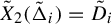 $\tilde {X}_2(\tilde {\Delta }_i)=\tilde {D}_i$
, and
 $\tilde {X}_2(\tilde {\Xi }_1)=\tilde {D}_{\Xi }$
.
Step 3. Preparation from inside. Now we consider the information in the diagonal region. We fix concentric round circles
 $E_i$
(
 $i=0,\ldots \pi (q)-1$
) in
 $D_q$
contained in the diagonal region of
 $F_{1,q}^{\pi (q)}$
such that:
-
• the center of
$E_i$
is q; -
•
$E_{i}$
is contained in
$E_{i-1}$
for
$i=1,\ldots \pi (q)-1$
; -
•
$E_{\pi (q)-1}$
contains
$E_{\pi (q)} :=F_{1,q}^{\pi (q)}(E_0)$
in its interior.


We denote their projections to
 ${\mathbb T}^2$
by
 $\tilde {E}_i \subset {\mathbb T}^2$
. Consider
 $\tilde {E}_i$
and
 $\tilde {C}_i$
in
 ${\mathbb T}^2$
(
 $i=0,\ldots , \pi (q)-1$
). Since they are in the same homotopy class in
 $D_q \setminus \{q\}$
, we see that they are ambient isotopic in
 ${\mathbb T}^2$
. We denote such an ambient isotopy by
 $\tilde {Y}_1$
(that is,
 $\tilde {Y}_1(\bigcup \tilde {C}_i) = \bigcup \tilde {E}_i$
holds).
Let us consider the position of the strong stable manifold
 $\tilde {\sigma }_j$
(
 $j=1, 2$
) in the orbit space. First, in each annulus
 $A_i$
(
 $i=0,\ldots ,\pi (q)-1$
), let
 $r_{1,i}$
(respectively
 $r_{2, i}$
) be the intersection between
 $A_i$
and the half x-axis in the positive (respectively negative) side. Similarly, using
 $A^{\prime }_i$
(
 $i=0,\ldots ,\pi (q)-1$
), we define
 $r^{\prime }_{1,i}$
and
 $r^{\prime }_{2, i}$
in a similar way.
Then, we choose two families of curves
 $\gamma _{i, j, k}$
(
 $j=1, 2$
,
 $k \in \mathbb {Z}$
) in
 $A_i \setminus A_{i+1}$
such that the following hold:
-
• in a small neighborhood of
$r^{\prime }_{i, j}$
,
$\gamma _{i, j, k}$
coincides with
$r_{i,j}$
; -
• in
$A_i \setminus A^{\prime }_i $
,
$\gamma _{i, j, k}$
winds k-times in the counter-clockwise direction (if k is negative, then it winds k-times in the clockwise direction); -
•
$\gamma _{i, 1, k}$
and
$\gamma _{i, 2, k}$
are disjoint.


Recall that
 $E_i$
are round circles in the diagonal region, and
 $E_i$
and
 $E_{i+1}$
bound an annulus. Consider the intersection of the annulus and
 $W^{ss}(q)$
. It is a union of two disjoint curves. We denote each connected component by
 $\sigma _{j, i}$
(
 $j=1, 2$
). Then, in
 ${\mathbb T}^2$
,
 $\tilde {\sigma }_{i, j}$
is a curve which connects
 $\tilde {E}_i$
and
 $\tilde {E}_{i+1}$
.
Now, we consider a diffeomorphism
 $\tilde {Y}_2$
which is isotopic to
 $\tilde {Y}_1$
satisfying the following:
-
•
$\tilde {Y}_2(\bigcup \tilde {C}_i) = \bigcup \tilde {E}_i$
; -
•
$\tilde {\sigma }_{i,j} \cap \tilde {A}^{\prime }_i$
coincides with
$\tilde {Y}_2(\tilde {r}^{\prime }_{i,j})$
; and -
•
$\tilde {\sigma }_{i,j}$
coincides with
$\tilde {Y}_2(\tilde {r}^{\prime }_{i,j})$
in a small neighborhood of
$\tilde {Y}_2(\tilde {r}_{i,j})$
.


Then we see that for each i,
 $\bigcup _{j}\tilde {\sigma }_{i,j}$
is ambient isotopic to
 $\bigcup \tilde {Y}_2(\tilde {\gamma }_{i, j,k_i})$
in the annulus bounded by
 $\tilde {E}_i$
and
 $\tilde {E}_{i+1}$
for some
 $k_i$
. Thus, we can take
 $\tilde {Y}_3$
which is isotopic to
 $\tilde {Y}_2$
satisfying all the conditions of
 $\tilde {Y}_2$
and
 $\tilde {\sigma }_{i,j} = \tilde {Y}_3(\tilde {\gamma }_{i, j,k_i})$
for every i and j.
Finally, we choose
 $\beta _i$
. Consider the annulus bounded by
 $E_i$
and
 $E_{i+1}$
. We choose a subset
 $\beta _i$
which satisfies the following. It is a rectangle whose edges are parallel to two coordinate axes and whose center is on the x-axis. Notice that
 $\mathrm {Int}(\beta _i) \cup W^{ss}(q)$
coincides with the x-axis. Now we perform the final modification to
 $\tilde {Y}_3$
. We take
 $\tilde {Y}_4$
which is isotopic to
 $\tilde {Y}_3$
, satisfying all the conditions of
 $\tilde {Y_3}$
and furthermore it satisfies:
-
•
$\tilde {Y}_4(\tilde {D}_i)$
is a disc contained in
$\mathrm {Int}(\tilde {\beta }_i)$
; -
•
$\tilde {Y}_4(\tilde {D}_{\Xi })$
is a disc contained in
$\mathrm {Int}(\tilde {\beta }_i)$
for some i.


Step 4. Estimation of the cost of the deformation. We have finished the preparation of the perturbation. Now we give perturbations to the family
 $(F_n)$
. In the following, the maps which will be perturbed are just
 $F_{n,F^{-1}(q)}$
.
As is in the argument of [Reference Bonatti and ShinoharaBS1
] (see the proof of [Reference Bonatti and CrovisierBS1
, Lemma 3.1]), we realize
 $\tilde {X}_2$
and
 $\tilde {Y}_4$
as follows. First, by applying the fragmentation lemma (see Theorem 6.6 in the next section), we take
 $C^1$
-diffeomorphisms
 $\{\tilde {\chi }_i\}_{i=1,\ldots , K}$
and
 $\{\tilde {\upsilon }_i\}_{i=1,\ldots , L}$
of
 ${\mathbb T}^2$
which are
 $\delta $
-
 $C^1$
-close to the identity and are supported on small discs such that the following equalities hold:
 $$ \begin{align*} \tilde{X}_2 = \tilde{\chi}_K \circ \cdots \circ \tilde{\chi}_1, \quad \tilde{Y}_4 = \tilde{\upsilon}_L \circ \cdots \circ \tilde{\upsilon}_1. \end{align*} $$
Now, consider the family
 $\{({\cal D}, F_n)\}$
, where
 $n = 3K+k+3L$
and
 $k\geq 1$
. We will prove the theorem setting
 $n_1 = 3K + 3L$
(for
 $n_1$
, see the statement of Proposition 6.3).
Step 5. Realization of deformations. In each three consecutive fundamental domains in the homothetic region
 $B(\unicode{x3bb} ^{3i-3}R) \setminus B(\unicode{x3bb} ^{3i} R)$
, we take the lift of
 $\tilde {\chi }_i$
and denote it by
 $\chi _i$
. We take
 $\tilde {\chi }_i$
in such a way that their supports are so small that we can take the lift of them supported in
 $B(\unicode{x3bb} ^{3i-3}R) \setminus B(\unicode{x3bb} ^{3i} R)$
.
Now consider the following diffeomorphism X of
 $D_q$
(whose support is contained in
 $B(R) \setminus B(\unicode{x3bb} ^{3K} R)$
):
 $$ \begin{align*} X = \chi_K \circ \cdots \circ \chi_1. \end{align*} $$
Since the conjugation by a homothetic transformation does not affect the
 $C^1$
-distance, X is also
 $\delta $
-
 $C^1$
-close to the identity map. We define the new IFS
 $({\cal D}, F^{\prime }_n)$
by composing X to
 $F_{n, F^{-1}(q)}$
and keep the other maps intact.
Now, there exist K,
 $K_0$
, and
 $n_1$
such that the following hold for every
 $n = n_1 +k$
:
-
•
$(F_{n,q}^{\prime \,\pi (q)})^{K_0}(\Lambda _i) = B(\unicode{x3bb} ^{K}\unicode{x3bb} _i R)$
for
$i=0,\ldots , \pi (q)-1$
; -
•
$F_{n,q}^{\prime \,\pi (q)}$
is a homothety of homothetic factor
$\unicode{x3bb} $
on
$B(\unicode{x3bb} ^{3K}R) \setminus B(\unicode{x3bb} ^{3K+k+3L}R)$
; -
•
$(F_{n,q}^{\prime \,\pi (q)})^{K_0}(\Delta _i)$
is a round disc contained in
$(F_{n,q}^{\prime \,\pi (q)})^{K_0} (\bar {\Lambda }_i \setminus \bar {\Lambda }_{i+1})$
disjoint from the x-axis and the line
$\{x=y\}$
; -
•
$(F_{n,q}^{\prime \,\pi (q)})^{K_0}(\Xi _1)$
is a round disc contained in
$(F_{n,q}^{\prime \,\pi (q)})^{K_0} (\bar {\Lambda }_{i_{\Xi }} \setminus \bar {\Lambda }_{i_{\Xi }+1})$
whose center is on the x-axis and disjoint from the line
$\{x=y\}$
.


We perform another perturbation. For
 $n=n_1 +k$
, take the lift of
 $\tilde {\upsilon }_i$
and compose it on
 $B(\unicode{x3bb} ^{3K+k}R) \setminus B(\unicode{x3bb} ^{3K+k+3L}R)$
and define Y in the similar way. That is, first, we take the lift of
 $\tilde {\upsilon }_i$
on
 $B(\unicode{x3bb} ^{3K+k+3(i-1)}R) \setminus B(\unicode{x3bb} ^{3K+k+3i}R)$
and denote it by
 $\upsilon _i$
(remark that
 $\upsilon _i$
does depend on k, while
 $\chi _i$
does not). Then consider the following diffeomorphism of
 $D_q$
:
 $$ \begin{align*} Y = \upsilon_L \circ \cdots \circ \upsilon_1. \end{align*} $$
Then for
 $F^{\prime }_n$
, we compose Y to
 $F^{\prime }_{n, F^{-1}(q)}$
and keep the other maps intact. We denote this IFS by
 $G_k$
.
We can check that it satisfies, in addition to the previous four conditions, the following ones:
-
•
$W^{ss}(q, F^{\pi (q)}_{n,q})$
coincides with the x-axis on
$B(\unicode{x3bb} ^{3K}\unicode{x3bb} ^{\ast }_iR) \setminus B(\unicode{x3bb} ^{3K}\unicode{x3bb} _{i+1}R)$
for every
$i=0,\ldots ,\pi (q)-1$
. Note that the same holds for
$B(\unicode{x3bb} ^{3K+j}\unicode{x3bb} ^{\ast }_iR) \setminus B(\unicode{x3bb} ^{3K+j}\unicode{x3bb} _{i+1}R)$
for
$j=0,\ldots , k-1$
; -
•
$(G_{k,q}^{\pi (q)})$
satisfies condition (P2) in Definition 6.1.


Thus,
 $(G_{k,q}^{\pi (q)})_{k \geq 1}$
is a retarded family for q and Q with a homothetic region
 $B(\unicode{x3bb} ^{3K}R) \setminus B(\unicode{x3bb} ^{3K+k}R)$
such that every
 $G_k$
is
 $\delta $
-
 $C^1$
-close to
 $F_{n_1+k}$
.
Final step. Taking conjugacy. Now, let us take a coordinate change between
 $D_q $
and
 $B(1)$
under which the family
 $(G_k)$
satisfies condition (P1) (we change coordinates only on
 $D_q$
). First, let
 $R_G = \unicode{x3bb} ^{3K}R$
be the radius of a ball such that
 $G_{k,q}^{\pi (q)}$
is a homothety on
 $B(R_G) \setminus B(\unicode{x3bb} ^{k}R_G)$
. Recall that
 $K_0 \geq 0$
satisfies
 $(G_{k,q}^{\pi (q)})^{K_0}(D_q) = B(R_G)$
. Then we define a family of diffeomorphisms
 $\{h_{k}$
} on the disc
 $B(\unicode{x3bb} ^{-K_0}R_G)$
as follows:
-
•
$h_k = G_{k,q}^{\pi (q)}$
inside
$(G_{k,q}^{\pi (q)})^{K_0}(D_q) =B(R_G)$
; -
• outside
$(G_{k,q}^{\pi (q)})^{K_0}(D_q)$
,
$h_k$
is a homothety of homothetic factor
$\unicode{x3bb} $
.


Now we can define a conjugacy
 $\rho :D_q \to B(\unicode{x3bb} ^{-K_0}R_G) $
between
 $G_{k,q}^{\pi (q)}$
and
 $h_k$
as follows. Set
 $\rho $
to be the identity map inside
 $(G_{k,q}^{\pi (q)})^{K_0}(D_q)$
. Outside
 $(G_{k,q}^{\pi (q)})^{K_0}(D_q)$
, we extend
 $\rho $
subject to the formula
 $\rho = h_{k}^{-1}\circ \rho \circ G_{k,q}^{\pi (q)}$
. Notice that
 $\rho $
can be extended to a conjugacy
 $\rho : D_q \to B(\unicode{x3bb} ^{-K_0}R_G)$
since
 $(G_{k,q}^{\pi (q)})^{K_0}(D_q) = B(R_G)$
.
Finally, by conjugating the family
 $\{h_k\}$
by the homothety with homothetic factor
 $\unicode{x3bb} ^{K_0}$
, we obtain the desired family. Notice that the conjugation by the homothety keeps the x-axis and the roundness of discs. Thus, we see that this conjugated family satisfies condition (P1). Using condition (P1) and the conditions on
 $(G_k)$
, we can also check that the resulted family also satisfies conditions (P2) and (P3). This completes the proof.
Remark 6.4. If we construct a prepared family by Proposition 6.3, then the obtained prepared family is automatically bounded, for
 $(F_n)$
are uniformly bounded and each
 $G_k$
is
 $\delta $
-close to
 $F_{k+n_1}$
.
In the rest of this section, we will prove the following.
Proposition 6.5. Let
 $\{({\cal D}, F_n)\}_{n \geq 1}$
be a prepared family for a periodic point q and its u-homoclinic point Q such that
 $(F_n)$
is uniformly bounded. For every
 $\varepsilon _2>0$
, there exist
 $n_0, m_0\geq 1$
and a neighborhood
 $W_{n_0}$
of q such that there is a family of adapted
 $\varepsilon _2$
-perturbations
 $(G_{m})_{m\geq m_0}$
of
 $F_{n_0}$
such that
 $G_{m}$
is a pre-solution of depth m and
 $(G_{m,q})^{\pi (q)}|_{W_{n_0}} = (F_{n_0,q})^{\pi (q)}|_{W_{n_0}}$
holds for every
 $m \geq m_0$
.
If we prove Proposition 6.5, then with Proposition 6.3, we can conclude Theorem 3.25. At the end of this section, we will prove Proposition 6.5 using Proposition 6.8, which will be proved in the next two sections.
6.2 Fragmentation lemma and the cost of a curve
In this subsection, we give an important ingredient of the proof of Proposition 6.5. First, let us recall the statement of the classical fragmentation lemma.
Theorem 6.6. (Fragmentation lemma)
Given any smooth closed Riemannian manifold M, any diffeomorphism
 $f\colon M\to M$
isotopic to the identity map, and any
 $\varepsilon>0$
, there is a sequence
 $\{ \varphi _i \}_{i=1,\ldots ,k}$
of diffeomorphisms of M with the following properties.
-
(1) For every i, the
$C^1$
-distance between
$\varphi _i$
and the identity map
$\mathrm {Id}_{M}$
is less than
$\varepsilon $
. -
(2) For every i,
$\varphi _i$
coincides with the identity map outside a disc of radius
$\varepsilon $
. -
(3)
$f=\varphi _k\circ \cdots \circ \varphi _1$
.


Theorem 6.6 enables us to decompose a given diffeomorphism into a composition of diffeomorphisms whose
 $C^1$
-distance from the identity is arbitrarily small, while it does not give any information about the number of diffeomorphisms needed. To prove Proposition 6.5, we need to establish the upper bound of it. To clarify the meaning of the upper bound, we introduce a definition.
Definition 6.7. Let
 $\gamma _1, \gamma _2$
be
 $C^1$
-curves in a disc
 $D \subset \mathbb {R}^2$
transverse to
 $\partial D$
. We assume that
 $\gamma _1$
and
 $\gamma _2$
coincide near
 $\partial D$
. Let
 $\eta>0$
. The
 $\eta $
-cost from
 $\gamma _1$
to
 $\gamma _2$
, denoted by
 $c_{\eta }(\gamma _1, \gamma _2)\in {\mathbb N}$
, is the minimum integer n such that there are diffeomorphisms
 $\varphi _1,\ldots ,\varphi _n$
of D satisfying the following:
-
•
$\varphi _i$
is supported in a disc of radius
$\eta $
contained in
$D \setminus \partial D$
for every i; -
•
$\varphi _i$
is
$\eta $
-
$C^1$
-close to the identity map for every i; and -
•
$\varphi _n\circ \cdots \circ \varphi _1(\gamma _1)=\gamma _2$
.


We will prove the following.
Proposition 6.8. Given a real number
 $\eta>0$
and a prepared family
 $\{({\cal D}, F_n)\}_{n\geq 1}$
for a periodic point q and its u-homoclinic point Q, there exist
 $c = c_{\eta }\in {\mathbb N}$
,
 $m_2 = m_{2, c}\in {\mathbb N}$
, and a curve
 $\gamma _0 \subset \Xi _1$
such that for every
 $n\geq 1$
and
 $m \geq m_2 + (n-1)\pi (q)$
, there is a curve
 $\gamma _{n, m}\subset \Xi _1$
which coincides with
 $\gamma _0$
near
 $\partial \Xi _1$
and satisfies the following (see Definition 5.8 for the definitions of
 $T_i$
,
 $S_i$
and
 $\Theta _i$
. Note that they are defined by
 $F_n$
and depend on n):
-
•
$\gamma _0 = \{x\mbox {-}\mathit {axis}\} \cap \Xi _1 =W^{ss}_{\mathrm {loc}}(q, F_{n,q}^{\pi (q)}) \cap \Xi _1$
; -
•
$\gamma _{n,m}\cap T_m = F_{n,q}^{\mathfrak {a}} \circ F_{n,Q}^{\mathfrak {t}} \circ F_{n,q}^{m}(W_{\mathrm {loc}}^{ss}(F^{-m}(Q_1)))$
(see §5.3 for the definitions of
$Q_1$
,
$\mathfrak {t}$
and
$\mathfrak {a}$
); -
•
$\gamma _{n,m} \cap \Xi _i$
is a connected
$C^1$
-curve and
$\gamma _{n,m}\cap \Theta _i=\emptyset $
for
$i=1,\ldots ,\mathfrak {t}-1$
; -
•
$\gamma _{n,m} \cap T_i$
is a connected
$C^1$
-curve and
$\gamma _{n,m}\cap S_i=\emptyset $
for
$i=0,\ldots ,m-1$
; -
•
$c_{\eta }(\gamma _{n, m}, \gamma _{0})\leq c$
for every
$n\geq 1$
and
$m\geq m_2+(n-1)\pi (q)$
.


The next lemma will be one of our main tools. We give a bound of the cost of curves in a simple situation. In the following, by
 ${\mathbb D}$
, we denote the unit disc
 $B(1) \subset \mathbb {R}^2$
.
Lemma 6.9. Let
 $0<\delta <1$
be given. Given
 $\alpha>0$
and
 $\varepsilon>0$
, there is
 $N\in {\mathbb N}$
satisfying the following property. Suppose
 $f\colon [-1, 1] \to {\mathbb R}$
is a
 $C^1$
-map satisfying:
-
•
$f(t)=0$
if
$t \in [-1, -1+\delta ] \cup [1-\delta , 1]$
; -
•
$|f'(t)| < \alpha $
for every t; -
• the graph of f, that is,
$\{(t, f(t)) \in {\mathbb R}^2 \mid t \in [-1, 1]\}$
, is contained in
${\mathbb D}$
.


Then there is a sequence of diffeomorphisms
 $\{\varphi _i \}_{i = 1,\ldots , K}$
where
 $K\leq N$
and satisfies the following:
-
• for every
$i=1,\ldots , K$
, the support of
$\varphi _i$
is contained in
${\mathbb D} \setminus \partial {\mathbb D}$
and has diameter less than
$\varepsilon $
; -
• for every i, the
$C^1$
-distance between
$\varphi _i$
and the identity map is smaller than
$\varepsilon $
; and -
•
$\varphi _K\circ \cdots \circ \varphi _1([-1, 1]\times \{0\})$
is equal to the graph of f.


Proof. Let
 $\theta \colon \mathbb {R}\to [0,1]$
be a smooth bump function satisfying the following:
-
•
$\theta $
is equal to zero in
$(-\infty , -2+\delta _0] \cup [2-\delta _0, +\infty )$
for some small
$\delta _0>0$
; -
•
$\theta $
is identically
$1$
on
$[-1,1]$
.


For every sufficiently large
 $n\in {\mathbb N}$
and every
 $i \in \{0,\ldots ,n^3-1\}$
, we denote by
 $\psi _{i,n}$
the diffeomorphism of
 ${\mathbb D}$
defined as the time one map of the vector field
 $$ \begin{align*}X_{i,n}(x,y)= \theta(n(y-\frac i{n^3}f(x)))\frac{f(x)}{n^3}\frac\partial{\partial y}. \end{align*} $$
Note that
 $\psi _{i,n}(x, i/{n^3} f(x))=(x, ({i+1})/{n^3} f(x))$
, so we have
 $\psi _{n^3-1,n}\circ \cdots \circ \psi _{0,n} ( (x,0) )= (x,f(x))$
for every
 $x \in [-1, 1]$
. Furthermore, the support of
 $\psi _{i,n}$
is contained in the
 $2n^{-3}$
-neighborhood of
 $\{(x, i/{n^2} f(x)) \mid x\in [-1+\delta ,1-\delta ]\}$
. A simple calculation shows that the
 $C^1$
-distance of
 $\psi _{i,n}$
from the identity map is bounded by
 $K \alpha n^{-2}$
(where
 $\alpha $
is the constant in the statement of this lemma and
 $K>0$
is some constant independent of f), and hence tends to
 $0$
when
 $n\to \infty $
.
However, the diameter of the support of
 $\psi _{i,n}$
does not tend to
 $0$
. To obtain this property, we take finer factorization in products of diffeomorphisms with smaller support.
We put
 $$ \begin{align*} \theta_{j,n}(x)= \frac{\theta(n(x- j/n))}{\sum_{k=-\infty}^{+\infty} \theta(n(x- k/n))}. \end{align*} $$
The family
 $\{\theta _{j,n}\}$
is a partition of unity whose differential is proportional to n. Then, we define diffeomorphisms
 $\{ \varphi _{i,j,n} \}$
as a time one map of the vector field
 $$ \begin{align*} X_{i,j,n}(x,y)= \theta_{j,n}(x) X_{i,n}(x,y). \end{align*} $$
Given a pair
 $(i,n)$
, each
 $\varphi _{i,j,n}$
commutes, because each
 $\varphi _{i,j,n}$
is, when restricted to the line
 $\{x=x_0\}$
, a flow generated by a proportional vector field. Let
 $\rho _{i,n}$
be the product of
 $\{\varphi _{i,j,n}\}$
for
 $j\in \{-2,\ldots , n +2\}$
. Then we have
 $\rho _{n^3-1, n}\circ \cdots \circ \rho _{0, n} ( (x,0) )= (x,f(x))$
for every
 $x \in [-1, 1]$
, the
 $C^1$
distance between
 $\varphi _{i,j,n}$
and the identity map is bounded by a constant proportional to
 $K'\alpha n^{-1}$
(where
 $K'>0$
is some constant independent of f) and the diameters of their supports are bounded by
 $4n^{-1}$
. Thus, the proof is completed.
6.3 Choice of the curves: proof of Proposition 6.8
Using Lemma 6.9, we can complete the proof of Proposition 6.8.
Proof of Proposition 6.8
Let
 $\{({\cal D}, F_n)\}_{ n\geq 1}$
be a prepared family for a periodic point q and its homoclinic point Q. Let
 $\unicode{x3bb} $
be the homothetic factor of the retarded family
 $(F_{n,q}^{\pi (q)})$
. Also, let
 $\eta>0$
be given.
To construct the family
 $\{\gamma _{n, m}\}$
, given
 $\eta '>0$
, we only need to construct a family of curves
 $\{\alpha _{n, m}\}_{n \geq 1, m \geq m_3+\pi (q)(n-1)}$
(where
 $m_3$
is some non-negative integer) in
 $D_q = B(1)$
such that the following hold (recall that
 $\Lambda _i$
and
 $\Delta _i$
are defined by
 $F_n$
, so they depend on n):
-
• let
$\alpha _0$
be the diameter
$D_q \cap \{x=y\}$
. Every
$\alpha _{n, m}$
coincides with
$\alpha _0$
near
$\partial D_q$
; -
•
$\alpha _{n, m} \cap \bar {\Lambda }_i$
is a connected curve for every
$i=0,\ldots ,m$
; -
•
$\alpha _{n, m} \cap \Delta _i = \emptyset $
for
$i=0,\ldots , m-1$
; -
•
$\alpha _{n, m} \cap (F_{n, q}^{\pi (q)})^i(\Xi _1) = \emptyset $
for
$i=0,\ldots , [m/\pi (q)]-1$
; -
•
$\alpha _{n, m} \cap \bar {\Lambda }_m$
coincides with the x-axis; -
• there exists an integer
$c_{\eta '}>0$
such that for every
$$ \begin{align*} c_{\eta'}(\alpha_{n,m}, \alpha_0) \leq c_{\eta'} \end{align*} $$
$n \geq 1$
and
$m \geq m_3 +\pi (q)(n-1)$
.


If we have constructed such a family, then we can obtain the conclusion. To see this, recall that there is an integer
 $\mathfrak {d}$
such that
 $T_{\mathfrak {d}} = F_{n,q}^{\mathfrak {a}}\circ F_{n,Q}^{\mathfrak {t}} \circ F_{n,q}^{\mathfrak {d}}(D_q)$
holds (see Remark 5.10, recall that
 $T_{\mathfrak {d}}$
is a disc in the transition well). If we take the image of the family
 $\{\alpha _{n, m}\}$
under
 $F_{n,q}^{\mathfrak {a}}\circ F_{n,Q}^{\mathfrak {t}} \circ F_{n,q}^{\mathfrak {d}}$
, it gives a family of curves in
 $T_{\mathfrak {d}}$
such that for each n, the
 $K_n\eta '$
-cost between
 $F_{n,q}^{\mathfrak {a}}\circ F_{n,Q}^{\mathfrak {t}} \circ F_{n,q}^{\mathfrak {d}}(\alpha _0)$
and
 $F_{n,q}^{\mathfrak {a}}\circ F_{n,Q}^{\mathfrak {t}} \circ F_{n,q}^{\mathfrak {d}}(\alpha _{n, m})$
is uniformly bounded, where
 $K_n>0$
is some constant determined by
 $F_{n,q}^{\mathfrak {a}}\circ F_{n,Q}^{\mathfrak {t}} \circ F_{n,q}^{\mathfrak {d}}$
. Note that
 $K_n$
depends on n, but as
 $(F_n)$
is uniformly bounded by assumption, the sequence
 $(K_n)$
is also uniformly bounded. As a result, the
 $K\eta '$
-cost of the family
 $F_{n,q}^{\mathfrak {a}}\circ F_{n,Q}^{\mathfrak {t}} \circ F_{n,q}^{\mathfrak {d}}(\alpha _{n, m})$
is uniformly bounded by
 $c_{\eta '}$
, where K is the uniform bound of
 $(K_n)$
. Thus, given
 $\eta>0$
, considering
 $\eta '$
satisfying
 $K\eta ' < \eta $
, we obtain the boundedness of the
 $\eta $
-cost for the image curves.
Let us explain how to extend these curves to obtain
 $\{\gamma _{n,m}\}$
and
 $\gamma _0$
. We extend the curve
 $F_{n,q}^{\mathfrak {a}}\circ F_{n,Q}^{\mathfrak {t}} \circ F_{n,q}^{\mathfrak {d}}(\alpha _0)$
to a
 $C^1$
-curve
 $\gamma _0$
in
 $\Xi _1$
which coincides with the x-axis near the boundary of
 $\Xi _1$
. Since the objects in
 $\Xi _1$
outside
 $T_{\mathfrak {d}}$
, such as
 $\Theta _i$
for
 $i=1,\ldots , \mathfrak {t} -1$
and
 $S_i$
for
 $i=1,\ldots , \mathfrak {d} -1$
, are the same for every n, we can extend each image
 $F_{n,q}^{\mathfrak {a}}\circ F_{n,Q}^{\mathfrak {t}} \circ F_{n,q}^{\mathfrak {d}}(\alpha _{n, m})$
to
 $\Xi _1$
such that the following hold:
-
• each extension coincides with
$\gamma _0$
near the boundary of
$\Xi _1$
; -
• the
$\eta $
-costs between each extension and
$\gamma _0$
are uniformly bounded; -
• the intersections between each extension and
$\Xi _i$
(
$i=0,\ldots ,\mathfrak {t} -1$
),
$T_i$
(
$i=0,\ldots ,\mathfrak {d}$
) are connected.


Thus, they give the desired family
 $\{\gamma _{n,m}\}$
.
Now, given
 $\eta '>0$
, let us construct the family of curves
 $\{\alpha _{n, m}\}$
in
 $D_q$
which has uniformly bounded
 $\eta '$
-cost from
 $\alpha _0$
. We only need to construct a family
 $\{\alpha _{1, m}\}_{m\geq m_3}$
since for general
 $\{\alpha _{n, m}\}$
, we only need to extend the homothetic image of
 $\{\alpha _{1, m}\}_{l\geq m_3}$
by a straight line in the homothetic region. Note that by increasing n by
 $1$
, the number of the homothetic region increases by
 $1$
, thus the number of intermediate strata increases by
 $\pi (q)$
. Thus,
 $\{\alpha _{n,m}\}$
is defined only for
 $m \geq m_3 + \pi (q)(n-1)$
.
Let
 $\tau $
be an integer in condition (P2) (see Definition 6.1). Recall that we have rectangles
 $\beta _k \subset \Lambda _{\tau +k} \setminus \Lambda _{\tau +k+1}$
for
 $k \geq 0$
. Now, we construct a family of curves
 $\{\zeta _i\}_{i \geq 0}$
in
 $\bar {\Lambda }_{\tau }$
satisfying the following conditions (see Figure 9):
-
•
$\beta _{k} \cap \zeta _i = \emptyset $
if
$k < i$
; -
•
$\beta _{k} \cap \zeta _i$
coincides with the x-axis if
$k \geq i$
; -
• for each i, the two endpoints of
$\zeta _i$
are
$\Lambda _{\tau } \cap \{x=y\}$
; -
• for every
$i \geq 0$
and
$j \geq \tau $
,
$\zeta _i \cap \bar {\Lambda }_j$
is a connected curve.


A graphical explanation of the family
 $\{\zeta _i\}$
. They are chosen in such a way that they have bounded derivatives with respect to the orthogonal
 $x'y'$
-coordinates where
 $\{x=y\}$
corresponds to the
 $x'$
-axis, except some finitely many
 $\zeta _i$
. In the picture,
 $\zeta _0, \zeta _1, \zeta _2$
are the exceptions. They need to turn back to reach the line
 $\{x=y\}$
and may fail to be graphs in
 $x'y'$
-coordinates.

Let us prove the following.
Claim 6.10.
 $\{ \zeta _i\} \subset \Lambda _{\tau }$
can be chosen in such a way that the
 $\eta '$
-cost from
 $\zeta _{-\infty } := \bar {\Lambda }_{\tau } \cap \{x=y\}$
is uniformly bounded.
Proof. We need to achieve two properties:
 $\zeta _i$
avoids the intersection with
 $\beta _k$
for
 $k < i$
and they must have intersection for
 $i \geq k$
. The other condition is that the intersection with
 $\zeta _i$
and
 $\bar {\Lambda }_j$
is connected.
To obtain both, we choose the family of curves
 $\{\zeta _i\}$
described as in Figure 9. Namely,
 $\zeta _{\ell }$
is a curve such that:
-
• in the positive x-half plane, first it follows the x-axis;
-
• then it makes an almost vertical turn to the y-direction between
$\beta _{\ell }$
and
$\beta _{\ell -1}$
; -
• after the curve reaches higher than the line
$\{ x= y\}$
, it makes another almost vertical turn to the x-direction. Recall that we require that
$\beta _i$
(
$i=0,\ldots \pi (q)-1$
) is disjoint from the line
$\{x=y\}$
; -
• when it arrives at the line
$\{x=y\}$
, the curve follows it to reach
$\Lambda _{\tau }$
; -
• on the negative x-half plane which contains no
$\beta _i$
, we just take some extension, paying attention to keep the condition about the connectedness.


We can construct such
 $\zeta _i$
for every sufficiently large i. If we introduce an orthogonal
 $x'y'$
-coordinate system on
 $\Lambda _{\tau }$
which sends
 $\zeta _{-\infty }$
to the
 $x'$
-axis, then it is not difficult to see that we can realize
 $\zeta _i$
as the graphs of functions whose derivatives are uniformly bounded. Note that in the diagonal region, the map
 $F_{1, q}^{\pi (q)}$
has the diagonal form. It guarantees that if the turns of
 $\zeta _i$
are sufficiently vertical, then the curves
 $\bar {\Lambda }_j \cap \zeta _i$
are connected.
Now, Lemma 6.9 implies the uniform boundedness of the cost from
 $\zeta _{-\infty }$
to
 $\zeta _i$
. There may be some curves where this construction does not hold, but there are at most finitely many such curves and their contributions are irrelevant to the boundedness of the cost.
Then we need to connect
 $\{\zeta _i\}$
to
 $\Lambda _0$
. The shape of
 $(\Delta _i)$
and
 $(F_{1,q}^{\pi (q)})^j(\Xi _1)$
may be complicated in
 $\bar {\Lambda }_0 \setminus \bar {\Lambda }_{\tau }$
but the size of this region is bounded. Thus, we can extend
 $\{\zeta _i\}$
to
 $\{\alpha _{1, m}\}$
keeping the uniform boundedness of the
 $\eta '$
-cost.
6.4 Proof of Proposition 6.5
In this subsection, we finish the proof of Proposition 6.5.
Proof. Let
 $\{({\cal D}, F_n)\}_{n \geq 1}$
be a prepared family and fix
 $\varepsilon _2>0$
. We take an integer
 $c>0$
and the curves
 $\gamma _0$
and
 $\{\gamma _{n,m}\}_{n\geq 1, m \geq m_2 + \pi (q)(n-1)}$
in
 $\Xi _1$
by Proposition 6.8. We have
 $c_{\varepsilon _2}(\gamma _{m, n}, \gamma _0 )< c$
for every
 $n \geq 1$
and
 $m \geq m_2+\pi (q)(n-1)$
.
By definition of the
 $\varepsilon _2$
-cost, for each
 $m \geq m_2+\pi (q)(n-1)$
, there are diffeomorphisms
 $\varphi _{1, m},\ldots ,\varphi _{c, m}$
supported in the interior of
 $\Xi _1$
,
 $\varepsilon _2$
-
 $C^1$
-close to the identity such that
 $$ \begin{align*}\varphi_{c, m}\circ\cdots\circ\varphi_{1,m}(\gamma_{n, m})= \gamma_0.\end{align*} $$
Fix now an integer
 $n_0$
greater than
 $c+1$
. We compose
 $\varphi _{i, m}$
to
 $F_{n_0,F^{-1}(q)}$
as in the proof of Proposition 6.3. Namely, for
 $i\in \{1,\ldots ,c\}$
, let
 $\psi _i$
be a diffeomorphism of
 $D_q$
which satisfies
 $\psi _{i, m}=(F_{n_0,q}^{\pi (q)})^i\circ \varphi _{i, m}\circ (F_{n_0,q}^{\pi (q)})^{-i}$
on
 $(F_{n_0,q}^{\pi (q)})^i(\Xi _1)$
and equal to the identity map outside. Note that
 $\psi _{i, m}$
is supported on
 $(F_{n_0,q}^{\pi (q)})^i(\Xi _1)$
, which is contained in the annulus
 $(F_{n_0,q}^{\pi (q)})^i(D_q) \setminus (F_{n_0,q}^{\pi (q)})^{i+1}(D_q)$
. Remark that this is contained in the homothetic region of
 $F_{n_0}$
.
Notice that the
 $C^1$
-distance between
 $\psi _{i, m}$
and the identity map is bounded by
 $\varepsilon _2$
, as
 $\psi _{i, m}$
is conjugated to
 $\varphi _{i, m}$
by a contracting homothety. The maps
 $\{\psi _{i, m}\}_{i=1,\ldots , c}$
have disjoint supports. So they commute. Let
 $\psi _m$
be the product
 $\psi _m=\psi _{c, m}\circ \cdots \circ \psi _{1,m}$
and let
 $G_m$
be a Markov IFS obtained by composing
 $\psi _m$
to
 $F_{n_0,F^{-1}(q)}$
and keeping the other maps intact.
The map
 $G_m$
is an admissible
 $\varepsilon _2$
-
 $C^1$
-small perturbation of
 $F_{n_0}$
. Let us check the following.
Claim 6.11.
 $G_m$
is a pre-solution of depth m.
Proof. Let us see that
 $$ \begin{align*} W^{ss}(q, G_{m, q}^{\pi(q)}) \cap \Xi_1 = \gamma_{n_0, m}. \end{align*} $$
Then, the fact that
 $G_m$
is an admissible perturbation of
 $F_{n_0}$
and the definition of
 $\gamma _{n_0, m}$
immediately implies the conclusion.
Consider a point
 $\bar x\in \Xi _1$
and
 $k>c$
. Then,
 $$ \begin{align*} (G_{m, q}^{\pi(q)})^k(\bar x) &=(F_{n_0,q}^{\pi(q)})^{k-c} \circ \bigg[\prod_{i=1}^c [(F_{n_0,q}^{\pi(q)})^{i}\circ \varphi_{i,m}\circ (F_{n_0,q}^{\pi(q)})^{-i} \circ F_{n_0,q}^{\pi(q)}] \bigg](\bar x) \\ &=(F_{n_0,q}^{\pi(q)})^k\circ\varphi_{c,m}\circ\cdots\circ \varphi_{1,m}(\bar x). \end{align*} $$
Therefore, for
 $\bar x\in \Xi _1$
, we have
 $\bar x\in W^{ss}(q,G_{m, q}^{\pi (q)})$
if and only if
 $\varphi _{c,m}\circ \cdots \circ \varphi _{1,m}(\bar x)$
belongs to
 $W^{ss}(q,F_{n_0,q}^{\pi (q)}) \cap \Xi _1 =\gamma _0$
, that is,
 $\bar x\in \gamma _{n_0,m}$
.
Thus, the proof of Proposition 6.5 is completed.
6.5 Weakness of the invariant curves
Now we are ready to finish the proof of Theorem 3.25. Let us complete it.
Proof. Let a Markov IFS
 $({\cal D}, F)$
with an
 $\varepsilon $
-flexible point q having a large stable manifold and its u-homoclinic point Q be given. Also, let
 $\eta>0$
and
 $\varepsilon _0>0$
be given.
First, we apply Lemma 5.6 and Proposition 6.3 successively. Then we obtain a bounded prepared family
 $\{({\cal D}, F_n)\}$
such that each
 $F_n$
is a
 $C^1$
-
 $\varepsilon $
-perturbation of F and the
 $C^0$
-distance between
 $F_n$
and F is less than
 $\varepsilon _0$
.
Then we apply Proposition 6.5 to
 $(F_n)$
letting
 $\varepsilon _2>0$
be small. Then we obtain
 $n_0$
,
 $m_0$
,
 $W_{n_0}$
, and a family of pre-solutions
 $(G_{m})_{m \geq m_0}$
of depth m which are
 $\varepsilon _2$
-admissible perturbations of
 $F_{n_0}$
. Each
 $G_{m}$
has a family of univalent invariant curves
 $\Gamma _m$
in
 $(0, m)$
-refinement by Proposition 5.12. Note that
 $(G_m)$
is bounded, too. Since
 $\varepsilon _2$
can be chosen arbitrarily small, we see that
 $(G_m)$
is
 $C^1$
-
 $\varepsilon $
-close to F and
 $C^0$
-
 $\varepsilon _0$
-close to F. Note that by shrinking
 $W_{n_0}$
, we may assume that the differential of
 $F_{n, q}^{\pi (q)}|_{D_q\cap W_{n_0}}$
on the x-axis is equal to one.
In the following, we will choose convenient m so that in the resulted dynamics, this curve has two kinds of hyperbolicity in the definition of contracting invariant curves, see Definitions 3.12, 3.13, and 3.15. We only explain how to establish the weakness of the curves. The choice of m for the contraction in the tangential direction is left to the reader.
We choose
 $$ \begin{align*} M_{+} &= \sup_m \Big\{\max_{x \in \Gamma_m} \|D(G_{m})^{-1}(x)|_{T{\cal D}/T\Gamma_m}\|\Big\},\\ M_{- } &= \inf_m \Big\{\min_{x \in \Gamma_m} \|D(G_{m})^{-1}(x)|_{T{\cal D}/T\Gamma_m}\|\Big\}. \end{align*} $$
Notice that, even though there are infinitely many maps
 $G_{m}$
in the argument of the supremum and the infimum,
 $M_{+}$
and
 $M_{-}$
are positive finite values, for
 $G_{m}$
are bounded. We apply Proposition 5.16 to
 $F_{n_0}$
, W, and some r. Then for every
 $G_{m}$
, the conclusion of Proposition 5.16 holds. In the following, we consider the case where the first conclusion of Proposition 5.16 holds, that is, there is one connected interval H satisfying the conditions. The proof for the second case is similar, so we omit the argument of that case.
Consider a point
 $x \in \Gamma _m$
for which
 $(G_{m})^{-m}(x)$
is defined. Since the normal expansion of
 $\Gamma _m$
is
 $1$
in W,
 $x \in \Gamma _m$
and x goes around
 $\mathrm {orb}(q)$
at least
 $([mr/\pi (q)] -2)$
-times (where
 $[x]$
denotes the integer part of x), we know
 $$ \begin{align*} &M_{-}^{m-([mr/\pi(q)] -2)\pi(q)} \leq \|D(G_{m})^{-m}|_{T\mathcal{D}/T\Gamma_m}(x)\| \leq M_{+}^{m-([mr/\pi(q)] -2)\pi(q)}. \end{align*} $$
Thus, by taking r arbitrarily close to
 $1$
, we see that the contribution of the derivatives outside W will be negligible. Thus, we have that the average normal derivative of
 $\Gamma _m$
tends to
 $1$
by letting r close to one.
7 On the proof of general cases
In this section, we discuss the proof of Theorem 3.24 based on the argument of the proof of Theorem 3.25. Indeed, the proof can be done in a parallel way, adding some modification to avoid the interference. Let us briefly see it.
Let
 $\{q_i\}$
and
 $\{Q_j\}$
be given.
-
• First, we apply Lemma 5.6 to each
$q_i$
. It gives us a saddle-node retarded family retarded at each
$q_i$
. Note that there is no interference between two different periodic points, due to the assumption of mutual separatedness. -
• Then, for each
$q_i$
, we consider the homo/heteroclinic points of
$\mathrm {orb}(q_i)$
. For each homo/heteroclinic point, we define the periodic well and the transition well in the first fundamental domain. -
• Note that two transition wells of different homo/heteroclinic orbits may share some discs, since two different homo/heteroclinic orbits may share their itinerary.
-
• However, they cannot have totally the same itinerary by assumption. Thus, at least we know that their periodic wells are disjoint.
-
• Now we give small perturbation to each retarded family which makes it to be prepared. Then for each periodic well, we find curves
$\{\gamma _{n, m}\}$
with bounded cost. -
• Since the periodic wells are disjoint, we have no interference when we perform the perturbation in §6.4. Thus, we can obtain the pre-solution of arbitrarily profound depth for each homo/heteroclinic orbits.


Acknowledgments
This work is supported by the JSPS KAKENHI Grant Numbers 18K03357 and 21K03320. K.S. is grateful for the hospitality of Institut de Mathématiques de Bourgogne of Université de Bourgogne during his visit.



