


Introduction
The aim of this paper is to investigate how uncertainty in modelled ice-sheet configurations is affected by a range of possible uncertainties in model inputs. In particular, we focus on assessing the influence of uncertainties in the representation of the bed topography in comparison with uncertainties of key mass-balance and ice-dynamic parameters input to a three-dimensional thermodynamically coupled ice-sheet model (ISM). We do this by carrying out parametric uncertainty analysis on these parameters, as well as applying modelled uncertainty to digital elevation models (DEMs) of an ice-sheet bed. Since our aim is to explore and compare uncertainty as a function of these parameters, model runs were carried out using a steady-state climate. The model runs explore ice-sheet extents and volumes in Fennoscandia, with mass balances approximately in line with the Last Glacial Maximum (LGM). However, we emphasize that we are primarily concerned with the development of methodologies to assess uncertainties in ISM results rather than the exploration of a particular ice-sheet reconstruction.
Uncertainty in ice-sheet models
Uncertainty in ice-sheet models has two main sources. Firstly, the modelled ice sheet is a function of the initial decisions made in abstracting the real system to a conceptual model. By abstracting reality, we are accepting that uncertainty will be inherent in the results of our model – users of numerical modelswill seektominimalizethis. Forexamplea model which does not consider longitudinal stresses will fail to replicate particular aspects of the glacial system. Secondly, model uncertainty can arise from uncertainties in the input parameters, such as the choice of parameter values at model initialization. The first set of uncertainties can only be explored through comparisons of systems that use different levels of abstraction in constructing their model rules. Thus, for example Reference Hubbard, Hein, Kaplan, Hulton and GlasserHubbard and others (2005) showed how the inclusion of longitudinal stresses led to considerable variation in modelled ice-sheet extents in Patagonia compared to previous results (Reference Hulton, Sugden, Payne and ClappertonHulton and others, 1994, Reference Hulton, Purves, McCulloch, Sugden and Bentley2002) based around models using the shallow-ice approximation (Reference NyeNye, 1957).
Within the ice-sheet modelling community, intercomparison experiments have sought to explore the sensitivity of modelled results to differences in implementation (and in principle abstraction). For example, the European Ice Sheet Modelling Initiative (EISMINT) experiments (Reference Huybrechts and PayneHuybrechts and others, 1996; Reference PaynePayne and others, 2000) explored a variety of model types and their responses to a range of glaciological (e.g. steady-state Greenland ice sheet under present conditions) and hypothetical experiments (e.g. ice-stream formation on a hypothetical symmetric topography). In many modelling fields a similar approach, though motivated by a different philosophy, is applied in ensemble modelling. Here, a variety of models are usually run in parallel and the results are weighted to provide a probabilistic forecast (Reference AndersonAnderson, 1996). Such approaches are arguably better suited for use in policy formulation, where the focus of interest is centred on risk estimation (Reference Vaughan and SpougeVaughan and Spouge, 2002).
In general, such model intercomparisons allow exploration of differences between models for a given scenario, and are important in moving models towards a consensus view. However, since intercomparisons are also often used as a benchmark towards which modellers aim in development, they cannot be said to be a means of quantifying uncertainty. Additionally, sensitivity to ‘external’ (input) parameters is not usually the subject of those intercomparisons, leaving a gap in the understanding of uncertainties associated with ice-sheet modelling, which we aim to fill. This second set of uncertainties, the focus of this paper, can be explored in a variety of ways. The most common approach employed in glaciological modelling is to carry out a sensitivity study. In such studies, all but one parameter are typically held constant whilst the parameter under investigation is varied through some range, and the response of the modelled ice sheet is visualized or quantified (e.g. Reference Van de Wal and OerlemansVan de Wal and Oerlemans, 1994; Reference Fabre, Letréguilly, Ritz and MangeneyFabre and others, 1995; Reference Ritz, Fabre and LetréguillyRitz and others, 1997; Reference Huybrechts and de WoldeHuybrechts and de Wolde, 1999; Reference Purves and HultonPurves and Hulton, 2000; Reference PattynPattyn, 2003; Reference Essery and EtcheversEssery and Etchevers, 2004). Sensitivity studies are important because they allow modellers to quantify which parameters, in isolation, have the greatest influence on model results. However, since all but the most trivial ice-sheet models are inherently non-linear, it is often difficult to properly quantify uncertainty or allow assignment of probabilities to particular outcomes (Reference Van der VeenVan der Veen, 2002).
Parametric uncertainty analysis
Currently, despite the increased importance of numerical modelling in policy making, relatively little research has explored ways in which uncertainties might be consistently calculated in individual ice-sheet model results. Parametric uncertainty analysis (PUA), where all parameters are varied together, is one such approach. Marshall and others (2002) investigated the response of the North America ice sheet to a range of parameters, and completed a number of simulations where parameters were varied simultaneously. Reference Tarasov and PeltierTarasov and Peltier (2004) also explored the response of the North American ice sheet during the LGM to simultaneous variations in a range of parameters, whilst geophysically constraining the modelled ice extents. However, in both these experiments the variation of parameter values appears to have been based on a limited variation of parameter values over a predefined range. Such approaches allow the range of potential model responses to input parameters to be estimated, but these responses are not associated with probabilities.
Reference Vaughan and SpougeVaughan and Spouge (2002) carried out a full parametric uncertainty analysis of future ice-sheet mass balance for the Greenland ice sheet using parameterizations of accumulation and ablation. A key difference in this approach is that probability density functions (PDFs) are estimated for each parameter, and used in the model runs to allow calculation of a final PDF for a chosen model output parameter. PDFs are, in general, used to associate a probability with a certain parameter value or model outcome. For example using a normal distribution as a PDF, values close to the mean are more likely to occur than values that deviate more from the mean – in the case of a normal distribution, 66% of all values are within one standard deviation of the mean. The advantage of using PDFs in parametric uncertainty analysis is that by including a (realistic) likelihood for a certain parameter value to occur, probabilities can be assigned to model outcomes. This, in turn, allows modellers, policy makers and users to identify in a more meaningful way how each parameter might affect the result, and estimate, for instance, the risk of extreme events. Typically, PUA is carried out using Monte Carlo simulation (MCS) which is a brute-force technique, where large numbers of model runs are normally required to generate an ensemble of results from which PDFs can be calculated.
Topography in ice-sheet models
In ice-sheet modelling the bed topography on which models are run is generally treated as having no uncertainty associated with it. However, the data used in the generation of these bed topographies is often associated with large uncertainties, which vary as a function of locale (Hebeler and Purves, 2008). Furthermore, the interpolation methods used to resample these data to resolutions appropriate for typical ISMs introduce further uncertainties (Reference Hebeler and PurvesHebeler and Purves, 2004). Topography, as discussed by Reference KerrKerr (1993), plays a key role in influencing ice-sheet behaviour through its geometry, whereby the mass-balance profile is controlled by relief (e.g. through orographic effects) and the topographic geometry (e.g. hypsometry). Topography also influences ice-sheet configuration directly by facilitating or constraining ice flow, for example in a glacial trough (Reference Jamieson, Sugden, Cooper, Barrett, Stagg, Storey, Stump and WiseJamieson and others, 2008). The sensitivity of modelled ice-sheet extents to uncertainty in topography is, thus, relevant to furthering our understanding of ice sheets, and to refining numerical models that seek to reconstruct such systems.
Aims
The objectives of this paper are, therefore, threefold:
-
1. to propose a generalizable set of methods for exploring the parametric uncertainty of ice-sheet model results;
-
2. to explore the influence of uncertainty in bed topography on modelled ice extents and volumes;
-
3. to compare the influence of topographic uncertainty to other sources of uncertainty (such as climatic or basal model inputs) on modelled ice extents and volumes.
The remainder of the paper is structured as follows. We briefly introduce the ice-sheet model used in our experiments, before we describe a method for exploring uncertainty in bed topography. We then review the parameters and associated PDFs derived for the parametric uncertainty experiments. The results of the experiments are presented as plots of ice extent and volume through time and by visualizations of ice extent and volume from ice sheets in equilibrium, using probability maps. Additionally histograms of the associated PDFs are given. Finally, we discuss the significance of the results and their implications for those constructing, using and interpreting ice-sheet models.
Methodology
The GLIMMER ice-sheet model
Physical laws relating to the dynamics of glaciers have long been incorporated into numerical models of ice flow, in order to make predictions about past, present and future ice-sheet behaviour (e.g. Reference Hulton, Sugden, Payne and ClappertonHulton and others, 1994; Reference OerlemansOerlemans and others, 1998; Reference Huybrechts and Le MeurHuybrechts and Le Meur, 1999). We aim to test how uncertainty in various model input parameters can affect the results of such ice-sheet models. To achieve this, we employ the community ice-sheet model GLIMMER (General Land Ice Model for Multiply Enabled Regions; Reference PaynePayne, 1999) which builds on the foundations laid down by the modelling studies of Reference HuybrechtsHuybrechts (1986), Reference Boulton and PayneBoulton and Payne (1993) and Reference Payne and DongelmansPayne and Dongelmans (1997). Ice dynamics calculations implement the shallow-ice approximation (Reference HutterHutter, 1983), a widely used approach which assumes that bedrock and ice surface slopes are small enough that normal stress components can be neglected. The ice flow law parameter is handled by a three-dimensional thermomechanical model. A full outline of the numerics implemented in GLIMMER is provided by M.K.M. Hagdorn and others (http://glimmer.forge.nesc.ac.uk), and Reference PatersonPaterson (1994) provides additional context to the derivation of these mechanics.
The ability of a modelled ice sheet to grow and interact with its bed and climate is strongly dependent on basal ice velocities. In GLIMMER, the velocities of the basal ice, v b, at any one point are determined as a function of the basal shear stress, τb, and the effective pressure (N = ice overburden pressure – basal water pressure) thus:

where k is a constant describing the thermomechanical properties of ice and p and q are positive integers (Reference PatersonPaterson, 1994). The basal slip coefficient, t b (also known as the basal traction parameter), determines the dependence of the thermomechanical properties of ice on N and therefore assumes that k and N −q can be integrated as a single parameter. Equation (1) can therefore be simplified (M.K.M. Hagdorn and others, http://glimmer.forge.nesc.ac.uk) to:

Sliding is assumed to occur when ice temperature at the bed reaches pressure-melting point (taking into account both a user-defined geothermal heat flux, G therm, and calculated frictional heat contributions), at which point the ice can detach from the bed and begin sliding due to the presence of water. Its ability to do so is a function of t b, which is calculated as a linear function of basal melt rate, b melt:

The slope of the function is given by t bslope, the softness of the bed is given by a parameter, b soft, and the basal traction is limited from becoming too large by the value of t bmax. Variability in the basal traction parameter will therefore alter the behaviour and form of the resulting ice mass.
At each time-step, the model requires spatial parameterization of surface mass balance and air temperature as inputs. We follow the approach of Jamieson and Sugden (2008) to generate these inputs. The distinction between snowfall (which only occurs below a given temperature, t snow) and rainfall across the model domain is determined using a positive degree-day (PDD) model (Reference ReehReeh, 1991). The PDD approach assumes that melt at the ice or land surface is proportional to the number of days (integrated through time) in which the air temperature, T, rises above freezing point. The number of PDDs is, therefore, proportional to the energy available for melting. Melt, w, is calculated by:
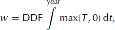
where DDF is the degree-day factor describing the density and albedo of snow or ice (DDF is different for each). The melt calculation further assumes that there is an annual sinusoidal cyclicity (i.e. seasonality) to air temperature, which is calculated by taking the mean annual temperature and an associated half-range, t range. Further diurnal deviations from the sinusoidally shifted mean annual temperature are accounted for by assuming that this variability has a normal distribution with a standard deviation of 5°C. The mean annual air temperature, MAAT, at the land or ice surface is calculated given a MAAT at sea level which is then adjusted to the surface using an atmospheric lapse rate, lrate. The model also incorporates a firn model to account for the fraction, w max, of melted snow that refreezes to become superimposed ice. The patterns of precipitation and MAAT used as inputs to this model are described under ‘Climate forcing’, below.
The Earth can be approximated as a thin elastic layer (the lithosphere) that floats above the asthenosphere. GLIMMER treats these two components separately and can do so in a number of ways. The flexural rigidity of the lithosphere is modelled as it responds to changes in load (Lambeck and Nakiboglu, 1980). The response of the asthenosphere to changes in overburden is modelled so mantle flow is approximated over time as an exponentially decaying hydrostatic response function (M.K.M. Hagdorn and others, http://glimmer.forge.nesc.ac.uk).
The model has been tested in the European Ice-Sheet Modelling Initiative (EISMINT) experiments (Reference Huybrechts and PayneHuybrechts and others, 1996; Reference PaynePayne and others, 2000) and it has been employed to gain better understanding of ice dynamics (e.g. Reference Le Brocq, Payne and SiegertLe Brocq and others, 2006). Furthermore, it has been used as a tool to reconstruct ice-sheet configurations over numerous regions and time periods (Reference PaynePayne, 1999; Reference Payne and BaldwinPayne and Baldwin, 1999; Jamieson and Sugden, 2008; Reference Lunt, Valdes, Haywood and RuttLunt and others, 2008).
Study area
For our experiments, we use basal topography of Fennoscandia extracted from 30 arcsec resolution GLOBE (Global Land One-Km Base Elevation) DEM data (http://www.ngdc.noaa.gov/mgg/topo/globe.html) between 50 and 72° N and between 14° W and 56° E. This is merged with ETOPO2 bathymetric data (http://www.ngdc.noaa.gov/mgg/global) at 2 arcmin resolution and transformed to Albers equal area projection. Thus the open water-bodies in GLOBE are filled by ETOPO2 data, and resampled to 10 km resolution. The model domain covers an area of 2580 km by 2370 km, with a minimum elevation of −3882 m and a maximum elevation of 1960 m.
Climate forcing
The primary objective of the experiments described in this paper is to investigate the influence of uncertainty in topography, climate and model parameters upon modelled ice-sheet extent and volumes. To this end, we are concerned with generating ice sheets in which parameters are varied and which can be compared to a benchmark simulation of a Fennoscandian ice sheet.
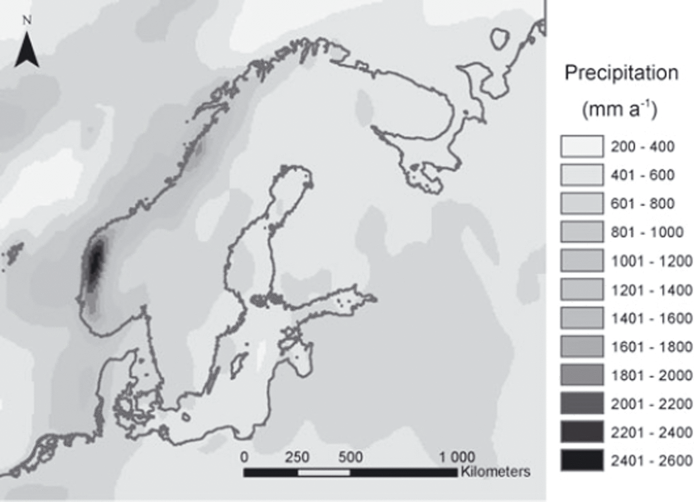
For precipitation rates, Climatic Research Unit (CRU; http://www.cru.uea.ac.uk) and Intergovernmental Panel on Climate Change (IPCC; http://www.ipcc-data.org/) observation data of recent climate were used to interpolate a precipitation scheme (Fig. 1), which can be scaled and varied over time. Notable features are high values of precipitation along the western coastal regions, with the highest precipitation of ∼2.6 m a−1 occurring in the southwest fjords.
Precipitation scheme for Fennoscandia compiled from present-day CRU and IPCC observation data serving as baseline input for the GLIMMER ISM.
CRU and IPCC climate data from 30 year observation periods were also used to compile MAAT at sea level for the study area. From this data, latitudinal dependencies were derived to construct an input temperature field at sea level that matches the general trends from observation data and gets colder with increased latitude. For modelling steady-state ice sheets on Fennoscandia, recent mean temperature was lowered by a constant value over the whole modelling domain (cf. Reference Huybrechts and de WoldeHuybrechts and de Wolde, 1999; Reference Forsström and GreveForsström and Greve, 2004).
Preliminary sensitivity tests for different temperature and precipitation schemes were run to determine an optimal climate set-up for the DEM uncertainty analysis as well as the parametric uncertainty tests. Lowering of present-day temperature by 10–14 °C, approximately resembling the cooling during the Last Glacial Maximum (Reference Ritz, Fabre and LetréguillyRitz and others, 1997), proved to produce stable and sensible ice-sheet extents.
DEM uncertainty experiments
DEMs are subject to uncertainties generated from sources such as resampling and data accuracy. GLOBE DEM data, commonly used for modelling in Fennoscandia, are known to contain substantial uncertainties originating from numerous data sources, from compilation methods and from measurement errors. Despite claims as to the need for detailed error models as an integral part of digital elevation data (Reference Ehlschlaeger and GoodchildEhlschlaeger and Goodchild, 1994), common DEMs such as GLOBE are distributed with only global error or accuracy figures (Reference FisherFisher, 1998) as described by the root-meansquared error, rmse (D.A. Hastings and others, http://www.ngdc.noaa.gov/mgg/topo/globe.html). These global accuracy figures have proven unrealistic and are of limited use as they lack information on the spatial distribution of error which is often spatially correlated with topographic attributes such as altitude or slope (Reference Holmes, Chadwick and KyriakidisHolmes and others, 2000; Reference Oksanen and SarjakoskiOksanen and Sarjakoski, 2005).
Therefore, in order to realistically model DEM uncertainty including spatial dependencies, higher-order reference data are necessary where no explicit error model exists. Because of the limited availability of such reference data for large regions of Fennoscandia, a model to simulate GLOBE DEM uncertainty has been developed (Hebeler and Purves, in press a,b). This model assesses GLOBE DEM error properties over a number of mountainous regions where higher-order reference data (A. Jarvis and others, Shuttle Radar Topography Mission (SRTM), http://srtm.csi.cgiar.org) are available. Using these regions, characteristics of error magnitude and spatial configuration, including their correlation with DEM characteristics such as elevation, slope and roughness, have been assessed. Analysis showed GLOBE error to be best modelled using deterministic components of uncertainty, modelled using regression, combined with stochastic elements. While the deterministic components reproduced the amount and spatial configuration of uncertainty well, the stochastic elements allow the produced uncertainty surfaces to be used within Monte Carlo simulations. The resulting uncertainty surfaces are essentially surfaces of deviations from the original elevation data in metres, and are added to the GLOBE DEM.
Using this uncertainty model, derived from areas with existing reference data, a suite of 150 uncertainty surfaces at 1 km resolution for Fennoscandia were produced. These uncertainty surfaces were then added to the original GLOBE DEM, resampled to 10 km and used as input to the GLIMMER ISM for Monte Carlo simulations, thus allowing assessment of the impact of GLOBE DEM uncertainty on ISM results. The baseline model set-up was used in our simulations, with present MAAT lowered by −10, −12 and −14°C, producing three sets of ISM runs. In order to determine the number of runs necessary to obtain stable and reliable results, the standard deviation of modelled ice extent across all model runs, and the standard deviation of this standard deviation, were plotted against the increasing number of runs, until both measures stabilized towards a constant value (Reference Raaflaub and CollinsRaaflaub and Collins, 2006). For each set, the mean and standard deviation of modelled ice extent and volume after 30 kyr (model years) across all runs were evaluated, and probability maps (Hunter and Goodchild, 1995) were compiled, as a measure of the frequency with which each cell was glaciated across a suite of Monte Carlo simulation (MCS) runs.
Parameter sensitivity
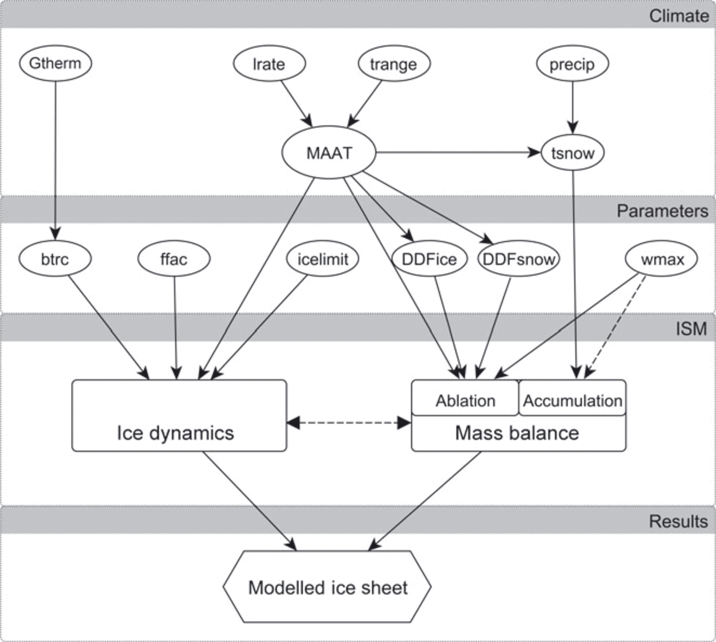
Using the PDD approach for determining snowmelt in GLIMMER, five parameters influence the temperature forcing. These are the mean annual air temperature at sea level, the latitudinal dependency of temperature, the seasonal variation of temperature, the atmospheric lapse rate and the geothermal heat flux. Additionally, four parameters influence the ISM via their explicit or implicit dependence on temperature, namely the degree-day factors for ice and snow, the threshold temperature for precipitation to fall as snow and the meltwater refreezing fraction (Fig. 2).
Relational diagram of the ISM parameters used in the sensitivity and parametric uncertainty analyses.
The following parameters were thus selected for initial sensitivity testing in order to identify sensible parameter ranges for PUA:
-
Mean annual air temperature and latitudinal dependency: MAAT
-
Atmospheric lapse rate: lrate
-
Annual temperature half-range (seasonal variation): t range
-
Precipitation: precip
-
Degree-day factor for ice: DDFice
-
Degree-day factor for snow: DDFsnow
-
Geothermal heat flux: G therm
-
Threshold temperature for precipitation to fall as snow: t snow
-
Meltwater refreezing fraction: w max.
The modelling of basal water and basal traction can influence ice-sheet configuration, because of their importance in controlling basal ice velocities. A flow enhancement factor is often used in ISMs as a tuning parameter to adjust ice-flow properties, for example, for layers of soft or warm ice. Thus, the following three additional parameters were tested, giving a total of 12:
-
Flow enhancement factor: ffac
-
Ice-thickness threshold for resolving physics: icelimit
-
Basal traction rate: btrc.
The influence of each of these parameters on mass balance and ice dynamics and their interrelations within GLIMMER are schematically depicted in Figure 2.
For all parameters, initial values, as well as variation ranges, were derived from the literature and are described in detail in the following section. Additionally, for climate forcing, variation was derived from uncertainty in the input data (e.g. using differences between CRU and IPCC data) and by accounting for uncertainty given in the respective metadata. Using information from the literature along with details of input data uncertainty and sensitivity, a probability density function (PDF) was derived for each parameter, to be used in the PUA. For this analysis, a suite of 510 input configurations for GLIMMER was created, where each of the 12 parameters listed above was randomly assigned a value according to the corresponding PDF.
Sensitivity Tests
In this section, the sensitivity tests using the selected model parameters are presented and discussed, and PDFs to be used within the PUA are deduced for each parameter.
Parameter ranges and PDFs
For each parameter the value range and selection criteria used within each sensitivity test are given here. A PDF to be used within the PUA for each parameter is deduced using the input criteria as well as the model sensitivity. An overview of both the tested parameter range and the resulting model sensitivity is given at the end of this section.
MAAT and latitudinal dependency
Differences found between the IPCC and CRU climate datasets used to derive MAATs lie in the range −5 to +7°C. This value range is similar to that reported by Reference Christensen, Christensen, Machenhauer and BotzetChristensen and others (1998) for CRU data compared with data from the Danish Meteorological Institute. Using these mapped differences as a basis, MAATs were varied in steps of 1°C for the sensitivity tests, spanning a range from 8 to 16°C cooling relative to present sea-level MAAT. Because the latitudinal variability of temperature is implicitly captured within the variation of MAAT compiled from the CRU and IPCC observations, model sensitivity to latitudinal temperature dependency was not explicitly tested and was kept constant for the PUA.
Probability distribution function for MAAT
Sensitivity tests for MAAT (Fig. 3a) revealed that temperature reductions of <8°C prevented any ice growth, because high ablation rates prevented ice nucleation at these temperatures. Temperature decreases of 9°C resulted in the formation of small ice caps, but high ablation rates still prevented the formation of larger ice sheets. For temperature reductions of >16°C, modelled ice sheets reached the borders of the modelling domain. Modelled ice extent after 30 kyr shows an almost linear dependency with temperature decreases between 9 and 16°C, thus indicating the relatively large influence of MAAT on model results within this range.
Sensitivity of modelled ice-sheet extents to variation in input parameters (a) MAAT, (b) seasonal temperature variation, (c) lapse rate, (d–f) precipitation at −10, −12 and −14°C (%), and (g, h) DDF for ice and snow (mm d−1°C−1).Sensitivity of modelled ice-sheet extents (solid curves) and volume (dashed curves) to variation in (i) geothermal heat flux, (j) snow threshold temperature, (k) refreezing fraction, (l) basal traction (as a function of basal melt rate), (m) flow enhancement factor and (n) ice-thickness threshold to solve ice dynamics.

The baseline scenario using a 12°C reduction from present-day temperature proved to give stable results for all parameter variations, so it was chosen as the mean for the MAAT PDF in the PUA. Because the probability of temperature scenarios above or below this mean should decrease towards the extreme ends of −8 and −16°C, a normal distribution with a standard deviation of 1.5°C (N[−12,1.5]) was chosen as the PDF for the PUA. Thus, 95% (the 2-standard-deviation range) of all temperatures lie between −9 and −15°C (Fig. 4a).
Probability distribution functions of the tested model parameters used in the parametric uncertainty function. (a) Mean annual air temperature, (b) seasonal temperature range, (c) lapse rate, (d) precipitation, (e, f) DDF for ice and snow, (g) geothermal heat flux and (h) snow threshold temperature. (i) Refreezing fraction, (j) maximum basal traction, (k) flow factor and (l) ice limit.

Seasonal temperature variation
To account for seasonal variation of air temperature, the MAAT imposed on the ISM is altered using a sinusoidal function with a default half-range of 9°C. This corresponds to an overall range in yearly mean temperatures of 18°C, a range characteristic of present-day maritime and semi-continental climates. According to Reference Christensen, Christensen, Machenhauer and BotzetChristensen and others (1998), current seasonal variation over Scandinavia ranges between 10 and 20°C. The seasonal temperature range, however, is known to be strongly dependent on continentality and MAAT, and thus can take on higher values for continental locations or lower ranges for extremely cold climates. For the initial sensitivity testing, seasonal temperature amplitudes between 3 and 15°C have therefore been used (Fig. 3b).
Probability distribution function for t range
Seasonal variation in temperature, t range, proved to have a large influence on ISM results. For the baseline approach with a 12°C temperature reduction, the variation of the seasonal temperature amplitude exhibited a non-linear dependency on the modelled ice extent. Because higher seasonal variations are more likely to raise temperatures above freezing, and thus cause ablation during parts of the year for a certain location, elevation threshold effects are likely to play a role in the sensitivity results (Hebeler and Purves, in press b). Variations in t range of 3–11°C resulted in stable, sensible ISM results. While slightly higher variations are still supported by the sensitivity results (Fig. 3b), a half-range of <3°C results in unrealistically large ice-sheet configurations. The seasonal temperature range amplitude was therefore varied according to a normal distribution around a mean of 9°C (N[9,2]). This yields a PDF with the 2-standard-deviation range (95%) between ∼5 and 13°C (Fig. 4b).
Lapse rate
The input temperature used to force ice-sheet growth is the air temperature at the upper surface. Surface elevation is equivalent to the bedrock elevation for ice-free areas (for glaciated areas ice thickness is added), and surface temperature is extrapolated from sea-level MAAT using an atmospheric lapse rate, which is commonly taken to be 6.5°C km−1 (Reference StoneStone, 1979). However, the moist adiabatic lapse rate is subject to seasonal and latitudinal variation as well as being dependent on height and atmospheric stability, and is suggested to be a better approximation to the atmospheric lapse rate in the middle and lower troposphere (Reference StoneStone, 1979). The lapse rate also varies with air moisture content, and increases up to 9.8°C km−1 for dry air. For cold, high-latitude regions, lapse rates have been shown to be fairly constant and nearly sub-moist adiabatic.
Air pressure, seasonal variation and temperature/precipitation dependencies of the lapse rate are not explicitly considered in our climate forcing. However, variation of the lapse rate for the sensitivity testing was chosen to reflect the maximum influence that these factors might have upon lapse-rate variability. Most models in very cold, dry environments, such as Antarctica, are generated using lapse rates of 7–9°C km−1 (Reference Thompson and PollardThompson and Pollard, 1997; Reference Van der VeenVan der Veen, 2002; Reference Jamieson, Sugden, Cooper, Barrett, Stagg, Storey, Stump and WiseJamieson and others, 2008). For their climate simulation, Reference Christensen, Christensen, Machenhauer and BotzetChristensen and others (1998) use a temporally variable lapse rate which ranges between 5 and 6°C km−1 across the year, and Reference Charbit, Ritz and RamsteinCharbit and others (2002, Reference Charbit, Ritz, Philippon, Peyaud and Kageyama2007) apply a lapse rate of 8°C km−1 for their model of the Fennoscandian ice sheet. Reference ReehReeh (1991) suggests a lapse rate of 8°C km−1 for polar regions. Given the uncertainty regarding appropriate lapse rates over different regions, we select the maximum and minimum previously used rates of 5–9°C km−1 for use in our sensitivity analysis (Fig. 3c).
Probability distribution function for lrate
Because of its direct relationship to temperature, modelled ice-sheet extent and volume is highly sensitive to lapse rate (Fig. 3c) within the tested parameterrange. An increase of the lapse rate from 5°C km−1 to 6.5°C km−1 almost doubles ice extent and volume, while a further increase to 8°C km−1 results in a smaller-magnitude response. Because of the cold climate conditions, the mean lapse rate for our experiment was assumed to be slightly higher than the commonly chosen value of 6.5°C km−1 and was set to 7°C km−1. For the PUA, a PDF based on a normal distribution around this mean of 7°C km−1 with a standard deviation of 1°C km−1 was selected (N[7,1]). The value range deduced from the literature (5–9°C km−1) is thus covered within the 95% interval of the PDF (Fig. 4c).
Precipitation
The range and distribution of precipitation derived from CRU and IPCC data compare well with those given by Reference Christensen, Christensen, Machenhauer and BotzetChristensen and others (1998). However, their reported bias of CRU precipitation data compared to observation varies for different regions by 15–30%. This range was used to derive values for initial sensitivity tests and served as a basis for parametric variation. Precipitation over Fennoscandia ranges from ∼0.4 to 2.5 m a−1, where most regions receive a mean of ∼1 m of precipitation. In order to preserve the spatial precipitation scheme, and to avoid unreasonably large changes to areas that had either high or low precipitation, precipitation rates for the sensitivity tests were scaled as a percentage of the derived baseline scheme.
For the sensitivity test, variations in the range −40 to +40%, relative to present-day distribution, were applied. As the impact of precipitation is strongly dependent on the mean temperature, sensitivity tests were conducted for three temperature scenarios, where recent MAAT was lowered by 10, 12 and 14°C, (Fig. 3d–f), in order to ascertain stable model runs for combinations of high precipitation rates and low temperatures.
Probability distribution function for precip
As expected, the impact of varying precipitation proved to be closely related to MAAT. Scaling of precipitation in the range −40 to +40% showed near-linear dependencies with modelled ice extent for the −10 and −12°C scenarios. For the −14°C scenario, the relationship became slightly non-linear, resulting in unstable model runs for increases in precipitation of >40%, for which ice reached the domain boundaries. Perturbing precipitation between −40 and +40%, however, produced stable equilibrium results for MAAT lowering between −10 and −14°C. The baseline precipitation was therefore used as the mean precipitation for the PUA PDF, and a global value for perturbing precipitation was drawn from a normal distribution around a mean of 0, with a standard deviation of 15% (N[0,0.15]) (Fig. 4d). This resulted in variations of precipitation between −30 and +30% in 95% of all cases. This slightly more conservative range was chosen to ensure model stability, while the 15% standard deviation still corresponds well, with a mean deviation of 20% of the CRU data, for the meteorological observations reported by Reference Christensen, Christensen, Machenhauer and BotzetChristensen and others (1998).
Degree-day factors for ice and snow
DDFs used for temperature-index modelling have been shown to vary for different regions, due to a range of factors such as seasonal and daily temperature amplitude, prevailing macroclimate, albedo and continentality. Where temperature-index models are used in glaciological modelling, different DDFs are commonly used for ice and snow. Reference HockHock (2003) compiled a list of snow and ice DDFs derived from a range of regional studies. DDFs for ice were shown to vary between 5.4 and 20 mm d−1 °C−1, with most values lying between 6 and 10 mm d−1 °C−1. Commonly, an average DDFice of 8 mm d−1 °C−1 is used for modelling ice melt, where DDFs cannot be derived from observations. The values compiled by Reference HockHock (2003) for DDFsnow range from 2.5 to 11.6 mm d−1 °C−1, with most values in the interval 3–6 mm d−1 °C−1.
For the sensitivity tests, the DDFs for ice and snow were varied between 6 and 10 mm d−1 °C−1 and between 3 and 8 mm d−1 °C−1, respectively.
Probability distribution function for DDFice and DDFsnow
Again, being closely related to temperature, variation of the DDFs has a large influence on the configuration of the modelled ice sheets (Fig. 3g and h). Increasing the DDF for snow from 3 mm d−1 °C−1 to 4 mm d−1 °C−1 results in a decrease of modelled ice-sheet extent and volume by ∼10% in the −12°C scenario.
For the parametric uncertainty analysis, the PDF for DDFice was centred around the standard value of 8 mm d−1 °C−1, which was used as a mean. A normal distribution with a standard deviation of 1 was used to cover the range identified in the literature, of 6–10 mm d−1 °C−1 (N[8,1]) within the 95% interval (Fig. 4e). As the standard value for DDFsnow marks the lower end of the variation range, an exponential distribution was chosen in this case, using a mean, μ, of 1 following the form

The default value of 3 mm d−1 °C−1 was added to the distribution, resulting in an effective range from 3 to ∼10 mm d−1 °C−1 and a mean of 4 mm d − 1 °C−1, covering the range of values from the literature with decreasing probabilities for extreme values (Fig. 4f).
Geothermal heat flux
For geothermal heat flux, most ice-sheet model experiments assume a value of 42 mW m − 2, which is a standard value for the average heat flux of Precambrian shields. However, Reference PollackPollack (1982) states that heat flux is dependent on the continental age and location. Reference Näslund, Jansson, Fastook, Johnson and AnderssonNäslund and others (2005) have calculated the average geothermal heat flux to be 49 mW m−2 for the Fennoscandian ice sheet, with regional variations ranging from 30 to 83 mW m − 2. In their sensitivity tests, Reference Ritz, Fabre and LetréguillyRitz and others (1997) also use values of 50 and 60 mW m − 2, the latter being the standard value for continents. Reference Greve and HutterGreve and Hutter (1995) vary the heat flux by ±30% in their Greenland sensitivity experiments, using values of 29.4, 42 and 54.6 mW m − 2. For our sensitivity tests, a variation of the geothermal heat factor of 35–65 mW m − 2 was chosen (Fig. 3i).
Probability distribution function for Gtherm
Ice velocity depends on the geothermal heat flux via the basal melt rates and resultant water pressures, which in turn determine rates of ice sliding. However, we find that changes in G therm have negligible influence on modelled ice extent and volume (Fig. 3i). For very cold MAAT, and thus low ice temperatures, the influence of geothermal heat on the thermal regime of the ice sheet is relatively small, which may explain the insensitivity to variation of this factor. However preliminary sensitivity tests with different temperature set-ups showed that variation of G therm within the given range could influence modelled ice volume, and therefore G therm was included in the PUA, and varied normally around a mean of 49 mW m − 2 using N[49,7] (Fig. 4g).
Snow temperature threshold
The threshold temperature, t snow, below which precipitation is assumed to fall as snow, thus contributing to accumulation for mass-balance modelling, varies little in the literature. For example, Reference Fabre, Ramstein, Ritz, Pinot and FournierFabre and others (1998) and Reference Charbit, Ritz, Philippon, Peyaud and KageyamaCharbit and others (2007) use a threshold of 2°C and Reference Schneeberger, Blatter, Abe-Ouchi and WildSchneeberger and others (2003) use a threshold of 1.5°C with linear interpolation of the rain/snow ratio from 0.5 to 2.5°C. Most other models employ a fixed threshold of 1°C. Sensitivity testing thus covered this range, between 0.5 and 2.5°C (Fig. 3j).
Probability distribution function for tsnow
The influence of the air temperature threshold for precipitation to fall as snow is slightly larger on modelled ice volumes than extents. Furthermore, we observe non-linear behaviour in our models due to the spatial distribution of precipitation, which results in local effects overlying global response patterns. This suggests that variation of the threshold temperature is a potentially important factor despite the relatively low overall impact compared to that of MAAT. For the PDF, the standard value of 1°C was assumed to have the highest probability. As the upper and lower end of the variation range are physically constrained, and are not symmetric around the mean of 1, a log–normal distribution (μ = 0.1, σ = 0.3) was chosen for the PUA, with maxima and minima constrained to 3 and 0.5, respectively. For simplicity, random values below 0.5 or above 3 were set to 1, hence the slight peak in the PDF (Fig. 4h).
Refreezing fraction
The refreezing fraction, w max, prescribes the amount of melted snow that refreezes to form superimposed ice. The default value of 0.6 thus states that the first 60% of snow melted by the potential ablation forms superimposed ice, while the rest is lost as runoff. The model is designed so that if potential ablation is greater than the volume of precipitation (as snow), superimposed ice melts first, before the ice itself. The ratio of 0.6 was used in a suite of papers on Greenland ice sheet modelling in the early 1990s (Reference Huybrechts, Letréguilly and ReehHuybrechts and others, 1991; ?; Reference Letréguilly, Reeh and HuybrechtsLetréguilly and others, 1991a). Even though some models and measurements suggest lower values might be appropriate or that no superimposed ice forms (e.g. Reference Lefebre, Gallée, Ypersele and GreuellLefebre and others, 2003), a ratio of 0.6 is commonly applied in the modelling of large ice sheets. We tested refreezing fractions of 0.4–0.8 for their impact on ISM results (Fig. 3k).
Probability distribution function for wmax
The refreezing fraction had a considerable influence when varied within the range tested (Fig. 3k), and is an important factor for uncertainty analysis. This is because as w max is applied globally over the model domain, it is uncoupled from influencing factors such as climate, ice rheology and topography. Within our PUA, the refreezing fraction is therefore varied around the standard value of 0.6 using a normal distribution N[0.6,0.065] (Fig. 4i).
Basal traction constant/basal sliding
In reality, since basal traction is dependent upon such factors as basal hydrology, the presence of deformable sediment or bedrock and basal sediment saturation (Reference Jamieson, Sugden, Cooper, Barrett, Stagg, Storey, Stump and WiseJamieson and others, 2008), one global constant is unlikely to represent the different conditions prevailing under an ice sheet. Basal traction specifies the dependence of the thermomechanical properties of ice on effective pressure. By prescribing basal traction as a function of basal melt rate, b melt, as we do here, spatial variations in the thermal field of the ice sheet become more gradual than if it were prescribed purely by the presence, or not, of water at the bed. Above a certain threshold of basal melt rate, basal sliding is at a constant maximum in our model. Reference Ritz, Fabre and LetréguillyRitz and others (1997) use a constant of 3 × 10 − 8 m a−1 Pa − 2; Reference PaynePayne (1995) applies a sliding multiplier of 5 × 10⁻³ m a−1 Pa−1; the standard value of the EISMINT experiments is 1 × 10⁻³ m a−1 Pa−1 (Reference PaynePayne and others, 2000). Reference Jamieson, Sugden, Cooper, Barrett, Stagg, Storey, Stump and WiseJamieson and others (2008) use basal traction constants of 2 × 10⁻³ and 5 × 10⁻³ m a−1 Pa−1 to explore ice-sheet behaviour. For our sensitivity tests, two different ways of calculating basal traction were used to test the importance of the inclusion of a basal melt rate parameterization. In a first approach, a constant basal traction value was applied where basal ice is at the pressure-melting point. This set of results was used to determine the range of basal sliding rates to test with the second approach, where basal sliding is a function of basal meltwater (Equation (3)). In this second sensitivity test, both minimum and maximum basal traction rates, t bmax, and the slope of the linear relationship between melt rate and basal traction, t bslope, were varied in order to determine optimal model set-up (e.g. Fig. 3l).
Probability distribution function for btrc
Changes in basal traction values have a considerable impact on ISM results and behaviour set-up, through their influence on model stability via velocity calculations. If basal sliding is modelled using a constant where basal ice is at its melting point (e.g. sliding and basal traction are set to either on or off), an initial increase from 0.1 × 10⁻³ m a−1 Pa−1 to 1 × 10⁻³ m a−1 Pa−1 results in growth of ice volume and extent. Increasing the basal traction constant then reduces both volume and extent, and triggers oscillation of the ice-sheet margins. This instability is due to the lack of transition between zero and maximum values of basal sliding, and was identified previously by Reference Payne and DongelmansPayne and Dongelmans (1997). For high basal sliding constants, this on/off scenario locally results in enhanced ice flow over the base which, in turn, results in a rapid drawdown of ice, which decreases ice thicknesses locally. This continues until a threshold minimum ice thickness and, in turn, driving stress is reached, whereby the warm streaming features shut down while ice thicknesses again build up, to a state where rapid flow can once again be initialized. Because of these instabilities, very high basal sliding rates (enabled by high btrc constants) do not lead to increases in overall ice extent. However, the impact of changes in basal traction very much depends on the method used for handling basal water in the ice sheet, and on local bedrock topography. If the basal sliding is modelled as a linear function of basal melt rate, with transition zones between areas of maximum and zero sliding, these instabilities are dampened, and the basal traction configuration has less influence on the modelled ice extent and volume (Fig. 3l).
While oscillating behaviour can be found in real ice streams, in ice-sheet models that do not account for longitudinal stresses it is likely to be a numerical artefact, especially where basal traction is uncoupled from basal melt rates (Reference Payne and BaldwinPayne and Baldwin, 2000). As model instabilities, which are the result of numerical limitations, can influence results, for the PUA a conservative set-up was chosen, using a (minimum) basal traction constant of 0.1 × 10⁻³ m a−1 Pa−1, a slope of 0.02 and variation of the maximum basal traction constant drawn randomly from a log–normal distribution (μ = 1e−05, σ = 0.75 (m a−1 Pa−1)), suitable for covering the wide range of possible values between 0.1 × 10⁻³ and ∼7 × 10⁻³ m a−1 Pa−1 (Fig. 4j).
Flow enhancement factor
A flow enhancement factor, ffac, is commonly used as a tuning factor. While a standard factor of 1 is often applied in ice-sheet models (e.g. Reference PattynPattyn, 2003), higher factors are often used to simulate changes in the physical properties of ice; for example, Reference Fabre, Letréguilly, Ritz and MangeneyFabre and others (1995) used this factor to represent layers of softer Weichselian ice in the Greenland ice sheet. In their sensitivity study of a Greenland ISM, Reference Ritz, Fabre and LetréguillyRitz and others (1997) used flow enhancement factors of 1, 3 and 5, values also used in previous experiments (e.g. Reference Huybrechts, Letréguilly and ReehHuybrechts and others, 1991; Reference Letréguilly, Huybrechts and ReehLetréguilly and others, 1991b; Reference Fabre, Letréguilly, Ritz and MangeneyFabre and others, 1995; Reference Greve and HutterGreve and Hutter, 1995). Sensitivity of ice extent and volume to flow factors of 0.5–5 has therefore been explored in our sensitivity tests (Fig. 3 m).
Probability distribution function for ffac
The sensitivity tests showed ice extent to be relatively insensitive to changes in flow factor, while the volume varied by up to 10% with each 0.5 point change in flow factor (between values of 0.5 and 1.5), while flow factors >2 have less effect on the ice volume (Fig. 3m). This effect can be explained by the lower viscosity of ice simulated through an increased flow enhancement factor. The ‘softer’ ice thus flows faster to lower elevations, where it is ablated, thus preventing the build-up of ice at higher elevations. This results in comparable ice extent yet decreased volume. Based on these results and the commonly used values for the flow enhancement factor, the PDF was chosen to vary around the default value of 1. As the parameter range of the flow factor around this standard value is asymmetric, a log-normal distribution was chosen for the PUA, with μ = 0.1 and σ = 0.36. The distribution was limited to a minimum of 0.5 by setting values below 0.5 to 1, hence the peak in the PDF plot (Fig. 4k).
Ice limit
For small ice thicknesses, only minimal deformation will occur, so the full thermodynamic equations need not be solved. For computational efficiency, a minimum ice-thickness threshold exists in GLIMMER, above which ice dynamics are solved. The default limit is 500 m, which corresponds to a maximum slope of 2.5% at 20 km resolution or 5% at 10 km. Using the shallow-ice approximation, it has been shown that ISMs become unstable when dealing with slopes >10%, corresponding to an ice-thickness change of 1000 m at the resolution of 10 km used in these experiments. Lowering the threshold results in an increased computational demand for little gain in the predictive ability of the model because flow rates at very low slopes are negligible. Sensitivity tests were thus performed using conservative thresholds of 200–600 m (Fig. 3n).
Probability distribution function for icelimit
As expected, changing the ice-limit threshold has little effect on the modelled configuration of ice sheets, while the calculation time significantly increased for low values (up to 30% for limits of 200 m instead of the default 500 m). However, variation of the ice limit results in non-linear behaviour, and has a slightly higher influence on modelled ice volume than on extents.
Despite the limited sensitivity of modelled ice masses to these effects, the ice-limit threshold is nevertheless included in the PUA for completeness. As no distribution can be deduced from the literature, and the parameter does not represent a physical process, a uniform distribution between 200 and 600 m was chosen for the PUA (Fig. 4l).
Results and discussion of sensitivity tests
The sensitivity tests conducted prior to the PUA indicate that the modelled ISM extent and volumes are most sensitive to input parameters that influence mass balance (see Fig. 2; Table 1): the tested range of mean annual air temperature (Fig. 3a) and seasonal variation in air temperature (Fig. 3b) resulted in the largest variations in modelled extent (up to 200%) in the sensitivity tests. Up to a 100% change was recorded for variation in precipitation for the −12 and −14°C scenarios (Fig. 3e and f). The impact of lapse rate (Fig. 3c), precipitation at −10°C (Fig. 3d) and the DDFs of ice and snow (Fig. 3g and h) was in the range 40–75%.
Sensitivity test parameters: default values of the baseline approach, tested parameter range and impact on modelled ice extent and volume. Impact is measured as the deviation range from the baseline (default) value after 30 kyr in per cent. Ratio is the ratio of relative impact of parameter variation on extent when compared to volume. Precipitation (m a−1) for each of the three temperature scenarios is varied in per cent relative to the baseline input scenario. Maximum basal traction is modelled using a slope of 0.02 for the basal melt function. Results of the DEM uncertainty test shown for comparison, with local maximum and minimum modelled uncertainty in metres, are discussed in the section ‘DEM uncertainty tests’
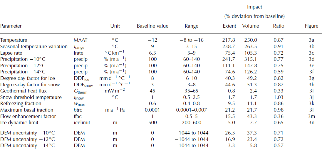
Model parameters that control ice dynamics have less influence over ice-sheet model results: variation of basal traction (Fig. 3l), the flow enhancement factor (Fig. 3m) and the refreezing factor (Fig. 3k) had an impact on modelled ice extent of ∼10–20%. Additionally, the variation of both the geothermal heat flux (Fig. 3i) and snow threshold temperature (Fig. 3j) parameters within their tested ranges was found to have limited influence on both modelled ice extent and volume (∼1–2%). Varying the ice-thickness threshold (Fig. 3n) for resolving of dynamics had a low to medium non-linear impact on model results, which varied by ∼5%. In general, the impact of changing the above parameters is slightly smaller on extent than volume.
While ‘external’ climate parameters have a greater influence on ice-sheet configurations, the ‘internal’ parameters that control ice dynamics can influence model stability, as shown by our sensitivity tests for different basal traction configurations. The effect these parameters have on model stability can be observed when examining ice-sheet behaviour. For example, particular selections of parameter values can generate oscillations in ice flow. Therefore parameter setups have been chosen that are unlikely to trigger model instabilities, and because of the use of these more conservative value ranges, the influence of internal ice-dynamics model parameters associated with internal ice dynamics might be low compared to the climate-forcing module.
While the strong influence of climate parameters concurs with previous findings (Reference Huybrechts and de WoldeHuybrechts and de Wolde, 1999), the sensitivity of modelled ice sheets to some other parameters is more controversial. For instance, Reference Huybrechts and de WoldeHuybrechts and de Wolde (1999) found basal melt rates had a large influence on the mass balance of the Antarctic and Greenland ice sheets, and melt rates of 10–30 m a−1 have been found for ice shelves (Reference Huybrechts and de WoldeHuybrechts and de Wolde, 1999; Reference Rignot and ThomasRignot and Thomas, 2002). For grounded ice, basal melt rates are heavily determined by the geothermal heat flux, and high basal melt rates under the Antarctic and Greenland ice sheets are explained by multiples of the normally assumed fluxes of 56 mW m−2. Reference Fahnestock, Abdalati, Joughin, Brozena and GogineniFahnestock and others (2001) report local basal melt rates of up to 1 m a−1 for the Greenland ice sheet. In our experiments, however, maximum basal melt rates lie in the range 0.5–1 m a−1, and variation of the geothermal heat flux showed little impact on modelled ice extent or volume, in agreement with the findings of Reference Ritz, Fabre and LetréguillyRitz and others (1997). This inconsistency could be explained by the conservative selection of parameter variation values, but since the applied values are averages over the whole modelling domain, higher rates appeared to be unreasonable and unsupported by the literature. Another possible explanation is that in our model set-ups, ice-thickness variation (and therefore topography) is a dominant factor influencing basal melt rates through overburden pressure. Because rapid variations in ice thickness are driving large differences in overburden pressure, they may overlay the impact of changes in geothermal heat flux. In this case, higher variations in G therm than the ones applied in our studies (which we assumed to be unrealistic) would show a greater impact on modelled ice extents and volumes.
Our experiments showed that increasing flow enhancement factors had a considerable effect on reducing modelled ice volume and, to a lesser amount, ice extent. In contrast, Reference Ritz, Fabre and LetréguillyRitz and others (1997) found a slight increase in modelled ice extent for initial increases of the flow factor for their Greenland experiments. Similar behaviour can be observed for variation in basal sliding comparing the two sets of experiments. Possible explanations may lie both in the topography and the climate configurations. For example, the Greenland ice-sheet margin positions are not only limited through high ablation in lower areas, but also by mass transport from the accumulation areas. In this case, the lower ice viscosity simulated by a higher flow factor would allow ice to flow further without being ablated. The relatively large seasonal temperature variations in our model set-up make it likely for an area to experience ablation during some time of the year, especially for lower elevations. Therefore increases in ice extent during colder periods of the year may ablate during the summer, and not contribute to the long-term expansion of the ice sheet.
The baseline parameters and their range examined in our sensitivity tests have been carefully compiled. However, both parameter ranges and parameter PDFs are approximations or are still based on assumptions. The impacts on modelled ice extent and volume of varying parameters across the ranges given in Table 1 are therefore not applicable for a direct comparison with each other or results from other studies. Nevertheless, the impact and the impact ratio (impact on extent/volume, measured as deviation from the mean in per cent) for each parameter can be used to compare the relative influence of each of the factors on ISM results. The derived impact ratio (Table 1) can also be used to determine whether parameters have a predominant influence on either modelled ice extent or volume. This is an important consideration in understanding the mechanisms through which these parameters influence the ISM.
In general, the impact ratio of parameter variation on modelled ice extent and volume is ∼0.8 (Table 1). This slightly higher impact of uncertainty on modelled ice volume can be explained by the fact that ice extent is a two-dimensional measurement. By contrast, the calculation of ice volume is three-dimensional and the variation of ice thickness is explicitly included. Because of the influence of topographic uncertainty on the calculation of ice thickness, its direct impact is likely to be reflected in modelled ice volume. Parameters with a low impact ratio have a greater influence on modelled ice volume than extent, such as the flow enhancement factor and the geothermal heat flux, via its influence on basal sliding. Both parameters influence ice velocity, through changes in either ice viscosity or sliding behaviour. Increased ice velocities support the accelerated flow of ice to lower elevations, where it is more likely to be ablated. At the same time, because ice flows away from the accumulation areas faster, ice build-up is inhibited. Thus, if mass-balance gradients at the edges of the ice mass are very steeply negative (i.e. high ablation rates occur near the equilibrium-line altitude (ELA)) then ice extent may not change significantly with increasing ice velocities. At the same time ice thickness (and thus volume) decreases because the ice transports ice from the accumulation zone to the ablation zone more rapidly.
Conversely, the maximum basal traction rate and the threshold temperature for precipitation to fall as snow have impact ratios close to 1 (Table 1). This means their influence on modelled ice extent is larger than on volume, when compared to other parameters. While the overall impact of t snow might be too small to support detailed analysis, it is interesting that higher rates of basal traction appear to favour changes in ice extent rather than volume. This is opposite to the effect of geothermal heat flux, a parameter that controls basal sliding via its dependence on basal melt. One explanation for this possible contradiction could lie in the fact that variation in geothermal heat flux affects the entire ice sheet, resulting in an overall change in the area of basal ice at its melting point. Changes in basal traction rate, however, only influence areas that already are at the pressure-melting point and are experiencing basal sliding. As this phenomenon occurs mostly in stream patterns and towards the edges of the ice sheet, where the ELA is positioned, changes in ice volume generated by the spatial pattern of ice velocity through basal traction may be relatively slow. At the same time, ice extent may be influenced more strongly through local advances of ice-stream outlets, because concentrated patches of thicker ice do not melt away as quickly as homogeneously distributed, but thinner, slow-moving ice advance. However, differences in, as well as overall values of, basal traction rate impact on modelled ice extent and volume are small, which means that small relative changes in model results can have strong influences on the associated impact ratio.
It is interesting to note the observable decrease of the impact ratio (Table 1) for the precipitation variation at −14°C. In comparison to the warmer climates tested, the impact upon volume versus extent increases. This may be due to the impact of air temperature on ice temperature and thus velocity. For the cold, −14°C, scenario, the ice-sheet boundary is strongly influenced by (low) ice velocities caused by the low temperatures as well as the high ice thickness dampening steeper slopes of the bedrock topography. This in turn results in areas of positive mass balance with increasing ice thickness, where ice cannot flow to ablation areas, so direct changes in mass balance mainly act on ice volume, rather than extent. Effectively, the stiffer, slower-flowing ice results in the build-up of a higher ice dome than the higher-temperature scenarios.
Parametric Uncertainty Analysis
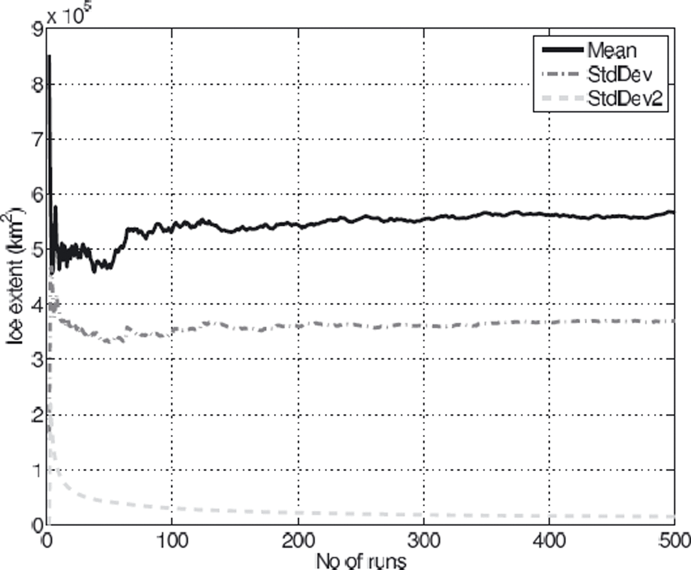
The mean modelled ice extent and volume across all 510 ISM runs comprising the PUA stabilized after ∼200 runs. However, variance in standard deviations of both extent and volume remained high, with >5% difference in standard deviation of modelled ice volume being generated between the 450th and 510th model runs. Analysis of the suite of ISM runs carried out for the PUA revealed that 6 out of the 510 configurations resulted in unreasonably large ice masses that reached the boundaries of the modelling domain, with ice extents >18 × 105 km2 (three times the standard deviation above the mean). All 6 configurations featured combinations of low temperatures (−14°C or lower) and small seasonal temperature variations, in conjunction with normal to increased precipitation rates. In 4 out of the 510 cases, the PUA configuration prevented the growth of any ice at all due to high temperatures (−7 to −9°C) and/or low precipitation. Upon removal of these 10 outliers, despite the high variance in input parameters, and the high sensitivity of modelled ISM results to these parameters, the variation in standard deviation of the modelled ice volume dropped below 5% after 200 runs (Fig. 5).
Mean (solid curve) and standard deviation (dashed curve) of ice extent after 30 kyr (model years) across PUA runs plotted against number of runs. Standard deviation of standard deviation is plotted as dashed light-grey curve.
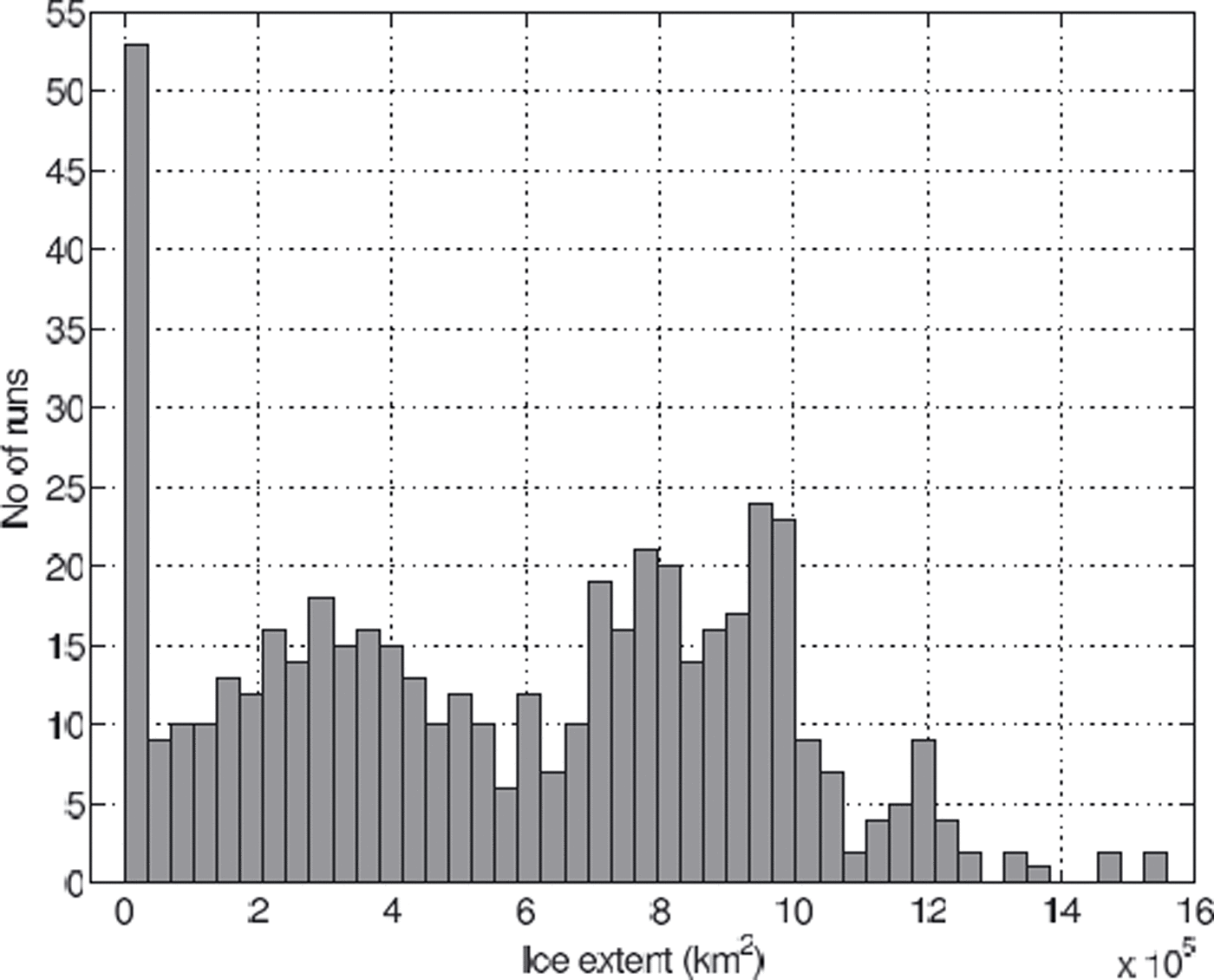
The small number of outliers (10 in total) comprise <2% of the runs, suggesting that PUA configuration was appropriate in most cases. The fact that only 6 configurations resulted in ice sheets that grew out of the domain suggests a conservative selection of parameter ranges towards their upper end. At the same time, the PDF plot (Fig. 6) shows >50 runs with ice extents <0.35 × 10⁵ km2, which essentially feature only a small number of glaciated mountain peaks and no significant ice sheets. This suggests the variation of input parameter ranges may be biased towards the lower end.
PDF of modelled ice extent of the parametric uncertainty analysis.
This is supported by the mean ice extent and volume of the PUA (Table 2), which lie below that of the −12°C baseline scenario (Table 3): the mean modelled ice extent of the remaining 500 ice sheets which reach equilibrium (after 30 kyr) is ∼5.7 × 10⁵ km2, with a standard deviation of 3.7 × 10⁵ km2, equivalent to slightly more than 65% of the mean (Table 2).
Mean, standard deviation (STD), maximum and minimum equilibrium (after 30 kyr) ice extent and volume for the PUA

Mean, absolute and relative standard deviation, maximum and minimum equilibrium ice extents and volume after 30 kyr (model years) for the three DEM uncertainty MCS scenarios, as generated after mean temperature lowering of 10, 12 and 14°C

Possible explanations for the smaller average ice extent compared to that of the −12°C baseline scenario include the unchanging spatial pattern of the precipitation scheme, where scaling of the precipitation below a certain threshold is more likely to inhibit ice nucleation in general. Another factor might be the PDFs of the input parameters. While most PDFs are symmetric around the default parameter values of the baseline configuration (e.g. MAAT, precipitation, lapse rate), the PDFs of DDFsnow, the flow enhancement factor and the snow threshold temperature (Fig. 4f, h and k) are asymmetric, with a higher probability of selecting values that result in relatively smaller ice sheets. However, the relatively low sensitivity of modelled ice sheets to these last three factors, and the high susceptibility to climatic factors makes it more likely the aforementioned ice-mass configurations are the result of high air temperatures and/or low precipitation.
Indeed, a closer examination of the model set-up configurations of the runs that resulted in no significant ice sheets showed that almost all of them had sea-level temperatures above −10°C (relative to present-day climate) in combination with high values of seasonal temperature variation. Sensitivity tests show that only small ice caps form for temperature lowering of <9°C (Fig. 3a), and, even for lower temperatures, high ablation rates during summer, as a result of large seasonal temperature variations, prevent the expansion of ice from the highest peaks. This underlines the fact that temperature is probably the most important parameter for the ISM, especially because it affects not only mass balance, but also ice dynamics, and has multiple feedback and coupling mechanisms (see Fig. 2).
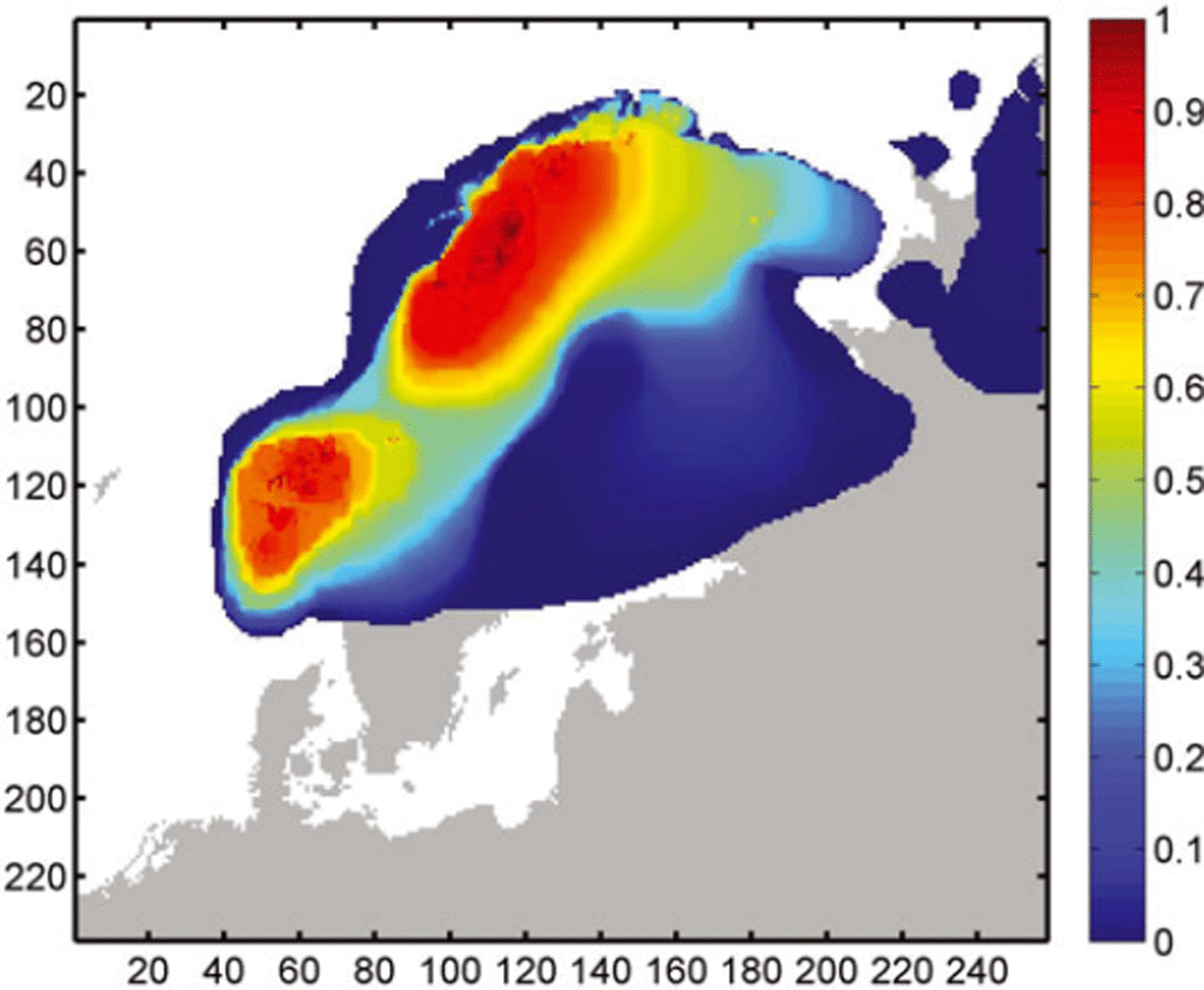
The model configurations generated for our PUA models cover a wide range of possible ice-sheet configurations (Fig. 7), and approximately half of all runs result in a single ice sheet stretching across the Fennoscandian ridge. This is reflected in a relative standard deviation of extent of 92% over all runs during the inception phases, which decreases with ice-sheet growth, and slowly increases again after 12 kyr to ∼65% (Fig. 8).
Probability map of modelled equilibrium ice extent across the PUA, showing likelihood of a cell being glaciated after 30 kyr across a suite of 500 model runs. Size of model area in cells is shown on the x and y axes.
Relative standard deviation (%) of modelled ice extent over time for PUA.

Apart from the peak in the PUA resulting from the runs where only small ice caps formed, the PUA shows a bifur cation of modelled equilibrium ice extent above and below 6 × 10⁵ km2. The probability map (Fig. 7) indicates that the cause is likely to be the coalescence of the two separate ice sheets in the northeast and southwest of the Fennoscandian ridge, which form in >80% of all runs. In ∼50% of all model runs, these two ice masses coalesce to form a single large ice sheet. Probability drops sharply to values <5% along the northwest coastal margin. A more gradual decrease is observed at the southeast ice-sheet margin in southern Sweden and towards the Russian mainland. A relatively small number of runs (<10%) show considerably larger ice sheets reaching further into the Atlantic and covering the Baltic Sea, as well as forming independent ice caps towards the eastern boundary of the modelling domain.
Dem Uncertainty Tests
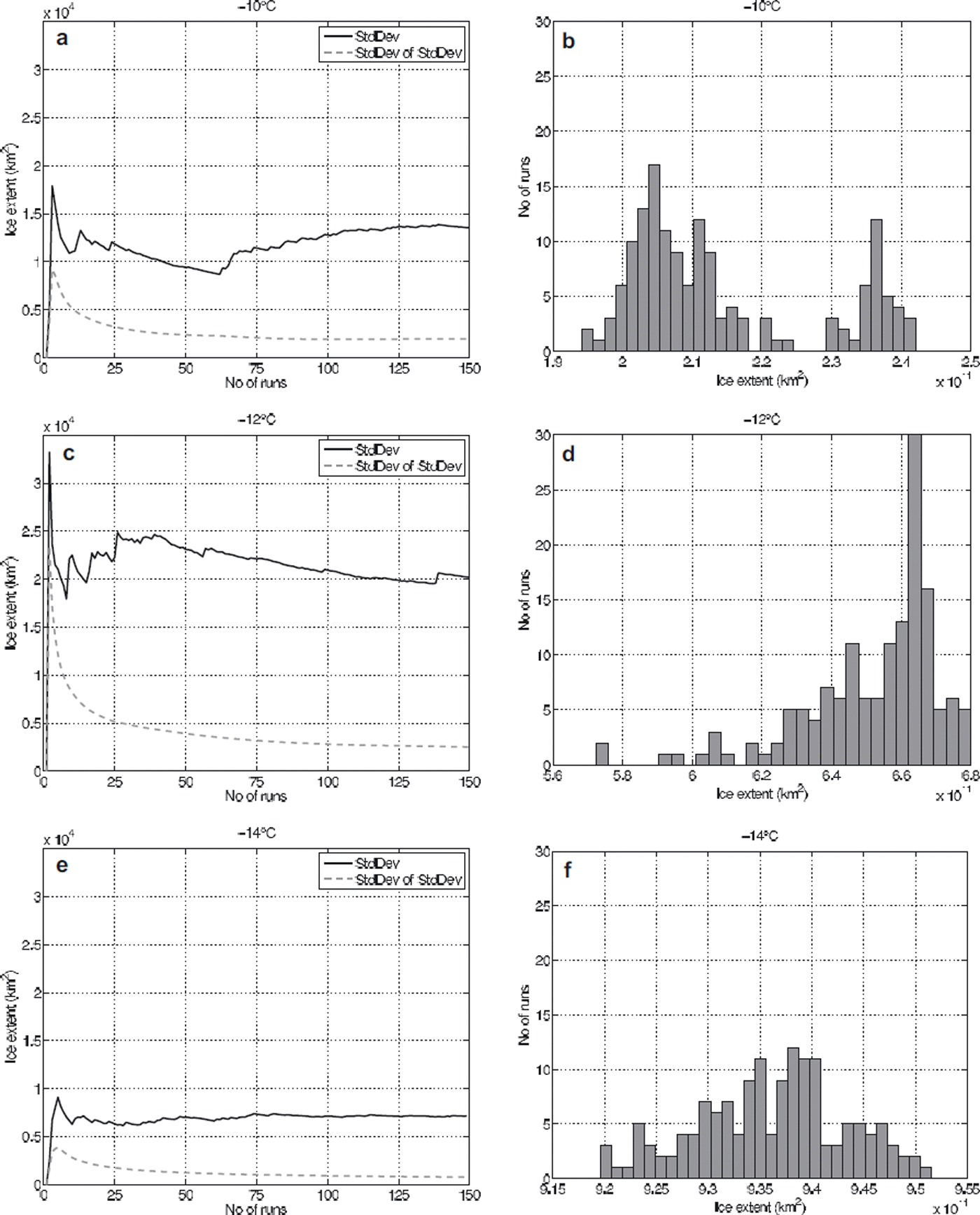
Plotting the standard deviation of the standard deviation of modelled ice extent against increasing numbers of MCS for the DEM uncertainty test shows the value stabilizes after ∼100–150 model runs under all three temperature scenarios (Fig. 9); consequently, the maximum number of conducted MCS runs for all scenarios was limited to 150. This number is considerably larger than the number of runs used in some other MCS. For example, Reference Davis and KellerDavis and Keller (1997) conducted 50 runs for slope stability prediction modelling, and Openshaw (1989) suggests 20–30 runs would be sufficient if only summary statistics are required. For our DEM uncertainty runs, an estimation of the mean of modelled ice sheets using only 50 runs would produce largely sensible results: the mean of the first 50 runs for the −10°C scenario is within 2.6% of that for all 150 runs (−12°C: 1.2%; −14°C: 0.3%). However an estimation of standard deviation after only 50 runs shows as much as 31 % change from the value derived after 150 model runs for the −10°C scenario (−12°C: 14.5%; −14°C: 1.8%; cf. Fig. 9). The requirement for an increased number of model runs to obtain a stable set of results is likely to be caused by the complexity of both the ISM and the model used to simulate DEM uncertainty, in comparison to, for example, a slope-stability model.
(a, c, e) The standard deviations of modelled ice extent across an increasing number of MCS runs for the −10, −12 and −14°C scenarios. Standard deviation of ice extent is plotted as solid curves, standard deviation of the standard deviation as light-grey, dashed curves. (b, d, f) The PDFs of modelled ice extents for the −10, −12 and −14°C temperature scenarios of the DEM uncertainty analysis using 30 equal-sized classes (note the different horizontal scales).
Modelled ice extent and volume for the three temperature scenarios (Table 3) show the total range of modelled ice extent (the difference between the minimum and maximum runs) to be ∼22% around the mean for the −10°C scenario, ∼16% for the −12°C scenario and ∼3% for the −14°C scenario. The variation for modelled ice volumes is notably higher, with values of ∼31, 23 and 6% for the −10, −12 and −14°C scenarios.
An increased cooling from −10°C to −12°C relative to recent temperatures results in an almost three-fold increase in modelled ice extent. The absolute standard deviation of modelled ice extents and volume under these cooler conditions only increases by about a third (Table 3; Fig. 9), which is equivalent to a drop of relative standard deviation from 6.6% to 3.1% (and equivalent to a drop from 9.1% to 4.2% in modelled ice volume). While further cooling to −14°C increases the size of the modelled ice sheet by about another 50%, absolute standard deviation also decreases and relative standard deviation drops to ∼1% (Fig. 10). The impact of DEM uncertainty as represented by relative standard deviation is larger for modelled ice volume than for ice extent.
Relative standard deviation (%) of modelled ice extent (solid) and volume (dashed) for the three temperature scenarios of the DEM uncertainty MCS.
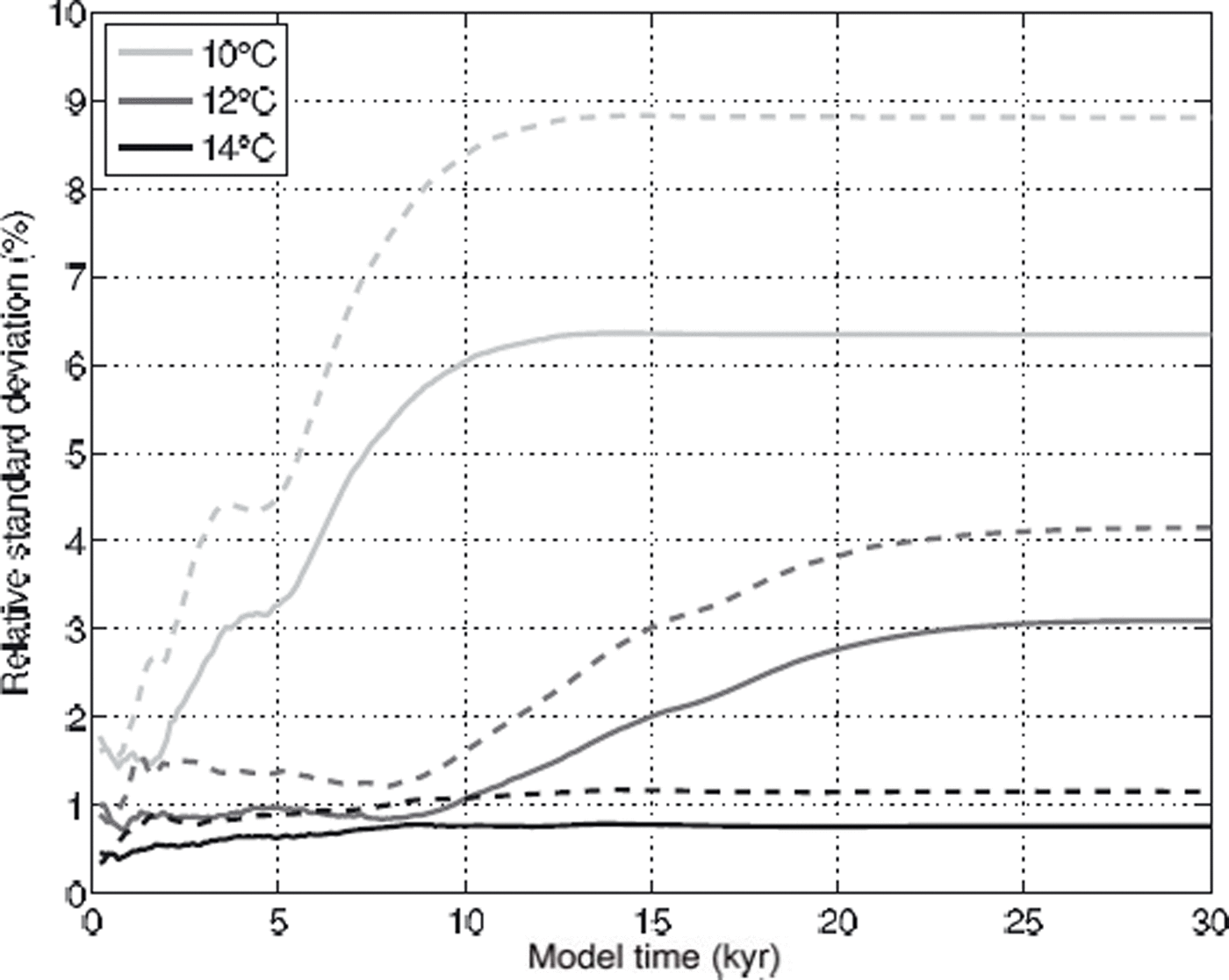
This decreasing impact of DEM uncertainty on ISM results with increasing total ice-sheet size, as measured by the relative standard deviation of ice extent and volume across MCS runs (Fig. 10), is consistent with previous findings (Hebeler and Purves, 2008), as is the larger impact of DEM uncertainty on modelled ice volume than on ice extent. These results reflect the shrinking influence of bedrock topography in models where ice-sheet configurations result in larger ice masses.
This fact is also supported by the probability distribution functions of modelled ice extent for the three temperature scenarios shown in Figure 9, which are classified into 30 equally distributed classes between the respective minimum and maximum modelled ice extent. In the −10°C scenario (Fig. 9b) a bifurcation in the PDF is observable, where a third of the modelled ice sheets are ∼20% larger than the rest.
Looking at the associated probability map for the −10°C set-up shows the main ice masses in northern Norway (Fig. 11a), with two smaller ice caps in the southwest with high glaciation probabilities. These are surrounded by an irregular probability distribution, showing that relatively large areas have relatively low probabilities of becoming glaciated. This suggests the bifurcation in the PDF is caused by the coalescence of the two southwestern ice caps. This occurs where local topography supports ice-mass coalescence, either by lowered elevation of obstructing ridges or by increased elevation of associated peaks, which can drive an increase in mass balance. The coalesced southern ice sheet can then expand further towards the east and west, due to the further increase in accumulation enabled by the presence of a high-elevation ice mass. This positive elevation mass-balance feedback occurs because as the two ice caps meet, the area between them is rapidly filled with ice, and instead of the bedrock, the elevated ice surface determines air temperature, resulting in increased likelihood of precipitation falling as snow and, in turn, less ablation, thus increasing the mass balance of the ice sheet. The additional ice then flows towards lower elevations, thus driving ice expansion in the west and east.
Probability maps of modelled ice extent of the DEM uncertainty MCS runs; (a) −10°C, (b) −12°C and (c) −14°C. Probabilityof each gridcell being glaciated across 150 runs is plotted on top of the Fennoscandian coastline. x and y axes are given in number of cells.
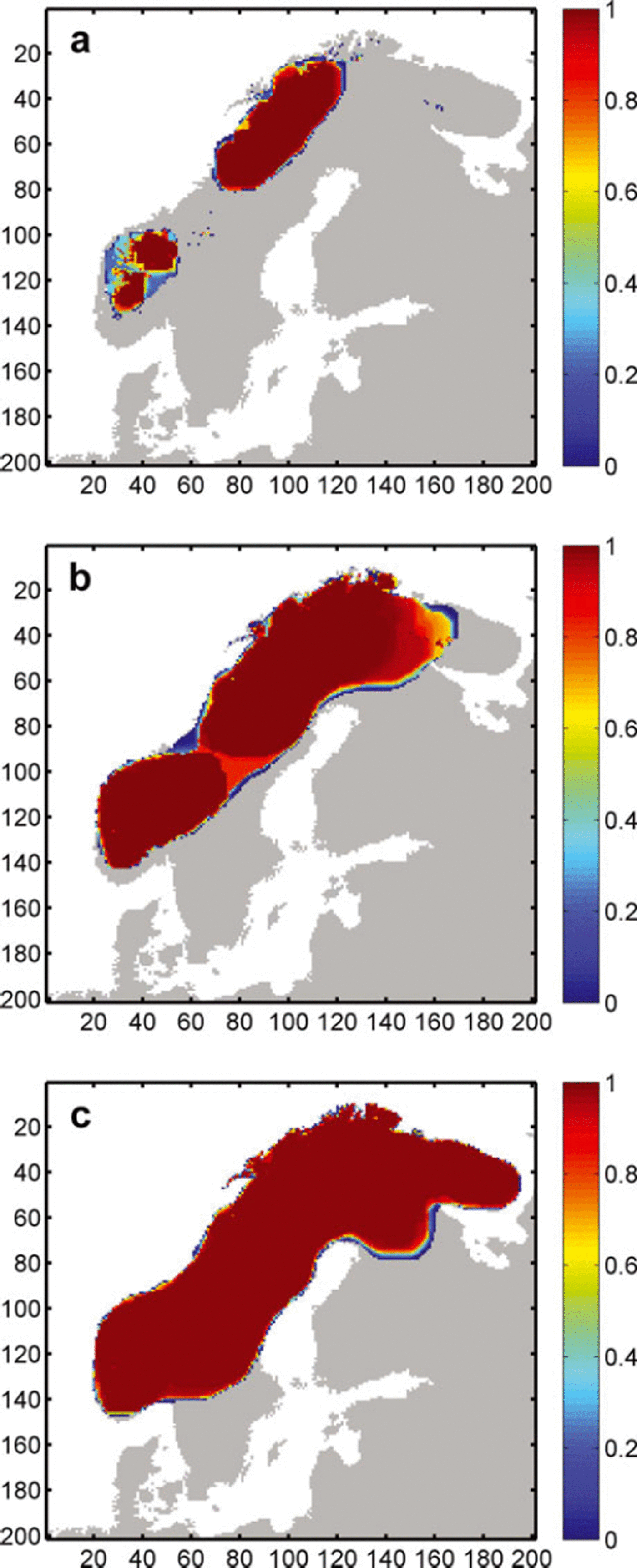
A clear peak and a slight right skew characterizes the PDF of the −12°C scenario (Fig. 9), with only nine runs featuring modelled ice extents of 10% or more below the mean. The associated probability map (Fig. 11b) features two glaciation centres, in the northeast and southwest, with glaciation probabilities being high over the majority of the potentially glaciated area but decreasing rapidly towards the ice margins, dropping to zero within an average range of ∼3–5 cells. This rapid transition of probability over a few cells indicates a relatively certain position of the ice margin. An exception to this is a considerable area of medium-to high-probability glaciated cells located between the northeastern and southwestern ice sheets. In ∼10–15 of the 150 runs, these ice sheets are not fully connected and the described elevation mass-balance feedback is not initiated, resulting in substantially smaller ice-sheet extents. This reflects uncertainty in the coalescence of the two ice masses. In the northeastern corner a similar pattern exists, where glaciation probability gradually decreases towards the ice margin over ∼20–30 cells. In these areas, the position of the ice margin is less certain, resulting in a higher sensitivity to uncertainty in bed topography. While, because of the large overall ice masses, the relative difference in size is comparably small, the configuration of the modelled ice sheets is significantly different, namely two separate ice sheets in almost 10% of all cases, as compared to a single large ice sheet.
With a further decrease in temperature to −14°C, the influence of DEM uncertainty, measured as both relative and absolute standard deviation, becomes negligible, resulting in an evenly distributed PDF with an absolute variation of 3.5% from the mean. The probability map for this scenario (Fig. 11c) shows a single ice mass stretching over the Fennoscandian ridge with centrally high probabilities of glaciation and, again, a rapid decrease in probability towards the edges. Here, ice extent is mainly limited by calving into the Atlantic and the Baltic Sea, as well as higher ablation rates in southern Sweden. The influence of topography on ice flow is limited to a relatively small area in the northeast, where the glaciation probability decreases more gradually towards the Russian mainland (Fig. 11c).
Since ice-sheet models are commonly run at resolutions of 5–20 km, an order of magnitude lower than the most common DEMs of the Earth’s surface (e.g. SRTM, GLOBE, GTOPO30), DEM accuracy is often assumed to be irrelevant. Our analysis has shown this assumption to be misleading, because uncertainty such as that simulated for the GLOBE DEM has an impact upon model results that is similar in scale to that of other key ISM parameters such as the flow enhancement factor, basal traction or the refreezing fraction. Additionally, because of the necessary resampling of DEMs during preparation for use as ISM input, key landform features and attributes are often lost due to the inherent smoothing. This, in turn, may lead to unrealistic tuning of an ISM or its climate-driver parameters in order to force ice growth.
Comparison of Results
The aim of this work is to systematically investigate the effect of uncertainty in model parameterization and input data, and to develop a set of methods that can be generalized for exploring this parametric uncertainty in ice-sheet model results, rather than to investigate the uncertainties associated with a particular ice-sheet reconstruction. The conducted model tests are valid primarily for the selected baseline parameter values, which makes a comparison of the absolute model results with those from other experiments, or with work from other authors, difficult. The main reason for this is that the impact of uncertainty in one parameter can strongly depend on a number of other model parameters. Modelling of the Fennoscandian ice sheet using different models, climate data or topographic resolution is likely to produce different results, which is partly triggered by the large degree of approximation applied in large-scale physical ice-sheet models. Despite this, a comparison of the results obtained throughout our experiments with empirical data, such as that compiled by Svendsen and others (2004), can help to integrate our findings with previous work.
In general, the ice-sheet configuration obtained by applying our baseline climate compares well with those compiled by Svendsen and others (2004) for the LGM in Fennoscandia, except for the eastern ice margin, where modelled ice sheets reach the Gulf of Bothnia and northern Finland, while the recorded LGM maximum is further east, reaching across the White Sea into Russia. The smaller ice sheets modelled within our experiments are presumably the result of the climate distribution (temperature and precipitation) based on present-day observations, which are likely to differ from those of the LGM. Additionally, because we did not aim at reconstructing the LGM ice sheet, boundary conditions were not adjusted for this task. Earlier experiments on Fennoscandia that applied climate time series based on Greenland Icecore Project (GRIP) data (Reference Dahl-JensenDahl-Jensen and others, 1998), as well as global sea-level changes, reproduced ice-sheet configurations well in line with recorded LGM extents (Reference HagdornHagdorn, 2003). Because open water of >250 m depth restrains ice advance through the associated calving rates applied within the model, the Baltic Sea prevents ice flow towards the east. Applying local sea-level lowering that prevailed during the LGM would have facilitated the filling of the Baltic Sea and consequent ice flow eastwards, and modelled ice sheets and associated uncertainties would have probably been larger. This assumption is sustained by the fact that for PUA runs with very cold climate and increased precipitation, which account for the maximum modelled ice extent (Fig. 7), the Gulf of Bothnia is ice-covered despite the unchanged sea level, and maximum ice extent reaches into the White Sea and Russia, giving a closer resemblance to the maximum ice limits mapped by Svendsen and others (2004).
While, for the DEM uncertainty experiments, the spatial distribution of the input topography was varied, for the PUA parameters were varied globally. The changes in topographic configuration as a result of DEM uncertainty influenced ice-sheet configuration both through impact on inception points and ice flow. Alteration of ridges and troughs controls the coalescence of ice masses and resulted in different configurations (two isolated vs one continuous ice sheet; Fig. 11a and b), represented by the bifurcation of the associated PDFs (Fig. 9). This same bifurcation can be seen in the PUA results (Fig. 6), where the influence of topography on ice-sheet configuration is determined by the prevailing climate. While the patterns are comparable, the variation of modelled ice extent and volume encountered in the PUA is much larger than that of the DEM uncertainty tests.
Conclusions
-
1. We have proposed a set of methods, that can be generalized, for exploring the parametric uncertainty of ice-sheet model results. The approach of compiling a range of possible parameter values from the literature as well as climate input data, and the derivation of associated probability functions to be used as input to a PUA, allows numerous stable models of ice sheets to be generated and analysed. While the 510 runs conducted for the PUA require considerable amounts of time and computing power, it was shown that if extreme outliers are eliminated during the analysis (e.g. through visual inspection) the overall number of necessary runs can be reduced to 200–250. Comparison of the relative impacts of tested parameters as well as their impact ratio on modelled ice extent and volume aids understanding of uncertainty impact mechanisms as well as the explanation of PUA results.
A comprehensive selection of ISM parameters were used to generate ice sheets of Fennoscandia, and the majority of these resulted in stable ice masses. This allowed us to identify the importance of particular parameters on ice-sheet extent and volume. The approach presented here provides a reproducible method for sensitivity testing of ISMs, in order to determine their susceptibility to uncertainty in input data and to the choice of model parameters.
-
2. Applying an uncertainty model in the simulation of DEM error allowed us to explore the impact of uncertainty in bed topography on modelled ice sheets. Across MCS runs, for ice sheets in equilibrium, recorded variations were in the range 0.8–6.6% for modelled extent, and 1.2–9.1% for modelled volume, depending on the applied temperature scenario. Even though these variations are relatively small, experiments suggest that the effect topographic uncertainty can have on model results, especially during phases of inception and for smaller ice sheets, is significant and can result in substantially different ice-sheet configurations. Using an ISM that employs the shallow-ice approximation in combination with a complex uncertainty model, such as the GLOBE DEM uncertainty model applied in this study, showed that a minimum of 100–150 MCS runs is required in order to deliver a stable and reliable set of results that inform the user about the probability of particular areas being glaciated.
-
3. Using different climate scenarios, the dependency of the impact of topographic uncertainty on the overall size of an ice sheet was determined. The influence of DEM uncertainty on ISM is comparable to that of (other) parameters, such as the flow enhancement factor or basal traction. Parameters influencing mass balance directly, such as mean annual air temperature, precipitation and DDFs, were confirmed to have the largest impact on modelled ice extent and volume. Uncertainty from model parameters, assessed by a full parametric uncertainty analysis, revealed large variations in modelled ice-sheet extents, with a relative standard deviation of 65% across MCS runs for equilibrium ice sheets. Modelled ice-sheet configurations exhibited a bifurcation, induced by characteristics of the bedrock topography.
Acknowledgements
This research was funded by the Swiss National Science Foundation SNF, project No. 200020-109449. We thank J. Fastook and an anonymous reviewer, as well as the scientific editor R. Greve, for help in improving this paper.



