1. Introduction
The fundamental properties of small-scale motions in turbulent flows can be described by the physical nature inherent to the velocity gradient tensor (VGT), e.g. the distribution of angles between the vorticity and the principal eigenvectors of the strain-rate tensor, the deformation of fluid elements, non-Gaussian characteristics and intermittency (Meneveau Reference Meneveau2011). In such a context, since the pioneering work of Vieillefosse (Reference Vieillefosse1982), the VGT has become an attractive research issue for studies aimed to interpret the turbulence dynamics (Ashurst et al. Reference Ashurst, Kerstein, Kerr and Gibson1987; Tsinober, Kit & Dracos Reference Tsinober, Kit and Dracos1992; Martín et al. Reference Martín, Ooi, Chong and Soria1998b; Wallace Reference Wallace2009; Wallace & Vukoslav $\breve{\rm c}$ević Reference Wallace and Vukoslavčević2010; Wang & Lu Reference Wang and Lu2012; Wang et al. Reference Wang, Wan, Chen, Xie, Zheng, Wang and Chen2020). The dynamic equation of the VGT can be derived from the Navier–Stokes equations, which comprise the nonlinear self-amplification term of the velocity gradient, the pressure correlation term and the viscosity correlation term. The pressure correlation term is usually expressed in the form of the pressure-Hessian tensor (
 ${\mathsf{H}}_{ij}=\partial ^2p/\partial x_i \partial x_j$), which reflects the non-local effect of turbulence and is the key to the sustainability of turbulence (Tsinober Reference Tsinober2009).
The extensive studies of VGT have significantly enriched the physical understanding of turbulence mechanisms for different turbulent systems. As is known, the flow topology indicated in the space of the VGT invariants is directly related to the local flow pattern in physical space, and different flow topologies have distinctive properties for the generation and dissipation of turbulent kinetic energy and enstrophy (Chong, Perry & Cantwell Reference Chong, Perry and Cantwell1990; Chacin & Cantwell Reference Chacin and Cantwell2000; Wang et al. Reference Wang, Wan, Chen, Xie, Zheng, Wang and Chen2020). Using the invariants of the VGT, Chacin & Cantwell (Reference Chacin and Cantwell2000) studied the generation of Reynolds stress, turbulent kinetic energy and dissipation in a turbulent boundary layer. Events corresponding to the strongest Reynolds stress and turbulent-kinetic-energy generation are found to occur mainly where the discriminant of the VGT has a rapid change of sign.
Chevillard et al. (Reference Chevillard, Meneveau, Biferale and Toschi2008) studied the geometrical alignments of vorticity with the eigenvectors of the strain-rate tensor and found that, in the region of unstable focus/compression (UFC) topology, the vorticity tends to be aligned with the first eigendirection of the strain-rate tensor. In incompressible jets, the alignment between the vorticity and the first eigenvector of the strain-rate tensor is observed for the stable node/saddle/saddle (SN/S/S) topology and stable focus/stretching (SFS) topology (Buxton & Ganapathisubramani Reference Buxton and Ganapathisubramani2010). Chu, Wang & Lu (Reference Chu, Wang and Lu2014) studied the generation of enstrophy in different flow topologies in compressible turbulent boundary layers. It is found that the SFS topology in the outer layer of the boundary layer contributes most to the generation of enstrophy, which depends on the alignment between the vorticity and the eigenvector of the strain-rate tensor. In the inner boundary layer, all flow topologies correspond to the positive generation of enstrophy. Recently, Wang et al. (Reference Wang, Wan, Chen, Xie, Zheng, Wang and Chen2020) studied the effects of flow topologies on the transfer of subgrid-scale kinetic energy in compressible isotropic turbulence. The results show that the unstable node/saddle/saddle (UN/S/S) topology and SFS topology play major roles in the forward transfer of subgrid-scale kinetic energy, while the unstable focus/stretching (UFS) topology corresponds to the inverse cascade of subgrid-scale kinetic energy.
Some valuable physical insights into the statistical properties of the pressure-Hessian tensor have also been obtained. The relatively early work can be dated back to Ohkitani (Reference Ohkitani1993) and Ohkitani & Kishiba (Reference Ohkitani and Kishiba1995) in which the three-dimensional Euler equations were studied numerically and analytically. They showed that the vorticity is a simultaneous eigenvector of the strain-rate tensor and the pressure-Hessian tensor. Kalelkar (Reference Kalelkar2006) studied the statistics of pressure fluctuations in incompressible decaying isotropic turbulence. It is found that the second eigenvector of the pressure-Hessian tensor tends to be preferentially parallel to the second eigenvector of the strain-rate tensor, and the first/third eigenvector of the pressure-Hessian tensor and the first/third eigenvector of the strain-rate tensor indicate a preferential relative angle of about  ${\rm \pi} /4$. The preferred ratio of the pressure-Hessian tensor's mean eigenvalues is
 $46:1:-47$ at cascade completion. By defining the cosine of the angle between the pressure-Hessian tensor and the strain-rate tensor, Holzner et al. (Reference Holzner, Lüthi, Tsinober and Kinzelbach2009) studied the geometrical effects and pressure–strain interaction in the proximity of the turbulent/non-turbulent interface. Chevillard et al. (Reference Chevillard, Lévêque, Taddia, Meneveau, Yu and Rosales2011) studied the statistical nature of pressure-Hessian effects in natural and synthetic fluid turbulence.
Lawson & Dawson (Reference Lawson and Dawson2015) examined the association of flow structure with VGT dynamics, and the modelling of fine-scale turbulent structure and its implications for VGT dynamics were explored. In compressible flow, pressure cannot be directly determined by the velocity field through Poisson's equation. It is an independent thermodynamic variable evolving via the state and energy equations. Therefore, the pressure-Hessian tensor exhibits more complex statistical properties (Suman & Girimaji Reference Suman and Girimaji2013). In compressible decaying isotropic turbulence, the statistics of the pressure-Hessian tensor are closely related to the dilatation rate. In the ‘incompressible region’ where the dilatation rate is nearly zero, the pressure-Hessian tensor's statistical properties are similar to those of incompressible turbulence. Besides, based on direct numerical simulations (DNS), Danish, Suman & Srinivasan (Reference Danish, Suman and Srinivasan2014, Reference Danish, Suman and Srinivasan2017) analysed the transport equation of the pressure-Hessian tensor in compressible decaying turbulence. They attempt to identify, isolate and understand the various inviscid mechanisms that affect the pressure-Hessian tensor's dynamics. As a result, the existing model of the pressure-Hessian tensor, namely the enhanced homogenized Euler equation (EHEE), was improved in their work.
The pressure-Hessian tensor plays a central role in the evolution of VGT dynamics. For incompressible flows, when the anisotropic part of the pressure-Hessian tensor and the viscous effect are neglected, the dynamic equation of the VGT degenerates to the restricted Euler (RE) equation with ‘finite-time singularity’ (Vieillefosse Reference Vieillefosse1982; Cantwell Reference Cantwell1992), which will lead to the divergence of the VGT. The deviatoric non-local part of the pressure-Hessian tensor, rather than the viscous term, is found to be responsible for counteracting the RE dynamics (Lüthi, Holzner & Tsinober Reference Lüthi, Holzner and Tsinober2009). To study the effect of the pressure-Hessian tensor on the evolution of VGT dynamics, one can investigate the conditional mean trajectory (CMT) of the second invariant ( $Q$) and the third invariant (
 $R$) of the VGT in the
 $Q$–
 $R$ plane and the contribution of off-diagonal terms of the pressure-Hessian tensor (Martín et al. Reference Martín, Ooi, Chong and Soria1998b). Previous studies illustrate that, in isotropic turbulence (Ooi et al. Reference Ooi, Martin, Soria and Chong1999; Chevillard et al. Reference Chevillard, Meneveau, Biferale and Toschi2008; Lüthi et al. Reference Lüthi, Holzner and Tsinober2009) and wall turbulence (Chu & Lu Reference Chu and Lu2013; Bechlars & Sandberg Reference Bechlars and Sandberg2017), the contribution of the pressure-Hessian tensor to the mean evolution of the VGT invariants is almost contrary to the action of the nonlinear self-amplification term, which counteracts the singularity of the RE equation.
To use simple ordinary differential equations to simulate the dynamic process of VGT, the key is to model the contribution of the pressure-Hessian tensor to eliminate the ‘finite-time singularity’ of the RE equation. Currently, there are several methods for establishing the models for VGT dynamics in isotropic turbulence, such as the stochastic diffusion model (Girimaji & Pope Reference Girimaji and Pope1990), the linear diffusion model (Martín, Dopazo & Valino Reference Martín, Dopazo and Valino1998a), the recent fluid deformation (RFD) closure (Chevillard & Meneveau Reference Chevillard and Meneveau2006), the Gaussian field closure (Wilczek & Meneveau Reference Wilczek and Meneveau2014; Johnson & Meneveau Reference Johnson and Meneveau2016) and the multiple-time-scale stochastic model (Johnson & Meneveau Reference Johnson and Meneveau2017), etc. Following the RE equation for incompressible flow, Suman & Girimaji (Reference Suman and Girimaji2009, Reference Suman and Girimaji2011) and Danish et al. (Reference Danish, Suman and Srinivasan2014) developed models for describing compressible VGT dynamics by the coupled evolution equations for the pressure-Hessian tensor and the VGT. However, these models are built based on the assumption of isotropic turbulence, and thus cannot be directly extended to inhomogeneous and anisotropic flows such as wall turbulence.
A deeper understanding of the influence of inhomogeneity and anisotropies on the pressure-Hessian tensor is the foundation for establishing a universal dynamic model for the VGT invariants. Till recently, study of the statistical properties of the pressure-Hessian tensor in wall turbulence has still been rare. In this study, the pressure-Hessian tensor's statistical properties in a turbulent channel flow and their effects on the dynamics of the VGT invariants are investigated by analysing DNS data of a weakly compressible turbulent channel flow. Firstly, the geometrical relationship between the pressure-Hessian tensor and the vorticity/strain-rate tensor in different flow topological regions is analysed. On this basis, the pressure-Hessian tensor's underlying mechanism on the evolution of invariant dynamics is discussed. The influence of inhomogeneity and anisotropy in the proximity of the wall is studied. Understanding the pressure-Hessian tensor's statistical properties in wall turbulence and its mechanism of action on invariants can provide helpful insight to model the pressure-Hessian tensor's contribution to the VGT dynamics for anisotropic and inhomogeneous turbulence.
The remainder of this paper is organized as follows: § 2 introduces the DNS database of turbulence in a channel and related calculation verification; § 3 introduces the VGT invariant and its dynamic equation; § 4 discusses in detail the statistical properties of the pressure-Hessian tensor and its mechanism of action on invariants; and § 5 gives a summary of this study.
2. The flow database and its validation
2.1. The flow database
To study the statistical properties of the pressure-Hessian tensor in wall turbulence, including the anisotropic and inhomogeneous effects, we adopted the flow fields of a weakly compressible turbulent channel flow with a bulk Mach number of  $Ma_B=1.56$ and a Reynolds number of
 $Re_B=7813$ based on the bulk-averaged velocity (Gerolymos & Vallet Reference Gerolymos and Vallet2014) in our previous paper (Tang et al. Reference Tang, Zhao, Wan and Liu2020). The corresponding frictional Reynolds number is
 $Re_\tau =532$. The implementation of the flow database is described briefly as follows. The Navier–Stokes equations governing the unsteady flow motions of a perfect gas are solved numerically by a seventh-order weighted essentially non-oscillatory scheme for the convection terms (Jiang & Shu Reference Jiang and Shu1996), an eighth-order central difference scheme for the viscous terms, and a three-step Runge–Kutta method for time advancement. This high-fidelity numerical strategy has been verified to reliably produce accurate results for compressible wall-bounded turbulent flows in previous work (Pirozzoli & Grasso Reference Pirozzoli and Grasso2004; Pirozzoli, Bernardini & Grasso Reference Pirozzoli, Bernardini and Grasso2008; Wang & Lu Reference Wang and Lu2012; Chu & Lu Reference Chu and Lu2013; Yu & Lu Reference Yu and Lu2020).
A computational domain of lengths  $L_x\times L_y\times L_z=4{\rm \pi} h\times 2h\times (4{\rm \pi} /3) h$ (
 $h$ is the channel half-height) in the streamwise (
 $x$), wall-normal (
 $y$) and spanwise (
 $z$) directions, respectively, is divided by the grid size of
 $N_x\times N_y\times N_z=800\times 300\times 600$. Uniform grids are used in the homogeneous (
 $x$ and
 $z$) directions, while the grids in the wall-normal direction are stretched to obtain the finest grid resolutions at the channel walls. Accordingly, the grid spacings in the streamwise and spanwise directions are
 $\Delta x^+=8.3$ and
 $\Delta z^+=3.7$, and the maximum and minimum grid spacings in the wall-normal direction are
 $\Delta y^+_c=5.5$ and
 $\Delta y^+_w=0.2$, respectively. In this paper, the superscript ‘+’ denotes the variables normalized by the wall unit variables. Periodic conditions are applied in the
 $x$ and
 $z$ directions. Standard isothermal, no-slip boundary conditions are applied at the channel walls. More details of the numerical procedures and validation can be found in Tang et al. (Reference Tang, Zhao, Wan and Liu2020). In the present channel flow, the turbulent Mach number is less than
 $0.3$, and the relative dilatation, which measures the local compressibility according to Suman & Girimaji (Reference Suman and Girimaji2013), is close to zero across the entire channel. Therefore, the compressibility is weak and its effects on the dynamics of the VGT can be ignored. This flow database is chosen to understand the fundamental properties of the pressure-Hessian tensor in the wall turbulence, with the effects of inhomogeneity and anisotropy to be the focus of this study.
2.2. Validation of the numerical results
The accuracy of numerical simulation is important for the study of the VGT. In particular, the dynamic equation of the VGT contains high-order derivatives, and it is crucial to reasonably capture those high-wavenumber components (Lozano-Durán, Holzner & Jiménez Reference Lozano-Durán, Holzner and Jiménez2015). This section first examines the budget equations of the turbulent kinetic energy (TKE) and the amplitude of the fluctuating VGT. Let the Reynolds decomposition of the variable  $f$ be
 $f =\bar {f} + f'$ and the Favre decomposition be
 $f=\breve {f}+f''$. In this paper, only flow data in the statistically steady state are chosen for analysis. The statistics are evaluated with both time averaging and space averaging in the homogeneous streamwise and spanwise directions.
The transport equation of TKE  $\breve {k} = \overline {\rho u''_ i u''_ i}/2\bar {\rho }$ in compressible turbulence is (Duan, Beekman & Martín Reference Duan, Beekman and Martín2011)
 \begin{align} {\frac{\partial\bar{\rho}\breve{k}}{\partial t}}&= \underbrace{-\frac{\partial\bar{\rho}\breve{k}\breve{v}}{\partial y}}_{C} \underbrace{-\overline{\rho u_i''v''}\frac{\partial\breve{u}_i}{\partial y}}_{P} \underbrace{-\frac{1}{2}\frac{\partial}{\partial y}\overline{\rho u_i''u_i''v''}}_{T} \underbrace{ -\frac{\partial}{\partial y}\overline{v''p'}+\overline{p'\frac{\partial u_i''}{\partial x_i}}}_{\varPi} \nonumber\\ &\quad +\underbrace{ \frac{\partial}{\partial y}\overline{u_i''\tau'_{iy}}}_{\varPhi_{dif}} \underbrace{-\overline{\tau'_{ij}\frac{\partial u_i''}{\partial x_j}}}_{\varPhi_{dis}} +\underbrace{\overline{u_i''}\frac{\partial \overline{\tau_{ij}}}{\partial x_j}-\overline{v''}\frac{\partial\bar{p}}{\partial y}}_{ST}, \end{align}
where  $u_i\ (i=1,2,3)$ (or
 $u,v,w$) are the velocities in the streamwise, wall-normal and spanwise directions,
 $\rho$ is density,
 $p$ is pressure and
 $\tau _{ij}$ is the viscous stress tensor. In the above equations,
 $C$ denotes the effect of mean convection on TKE,
 $P$ is the generation term of TKE due to the mean shear flow,
 $T$ is the turbulent transport,
 $\varPi$ is the pressure term including pressure diffusion and pressure dilatation,
 $\varPhi _{dif}$ and
 $\varPhi _{dis}$ are viscous diffusion and dissipation terms, respectively, and
 $ST$ represents the generation of TKE caused by the inhomogeneity of density.
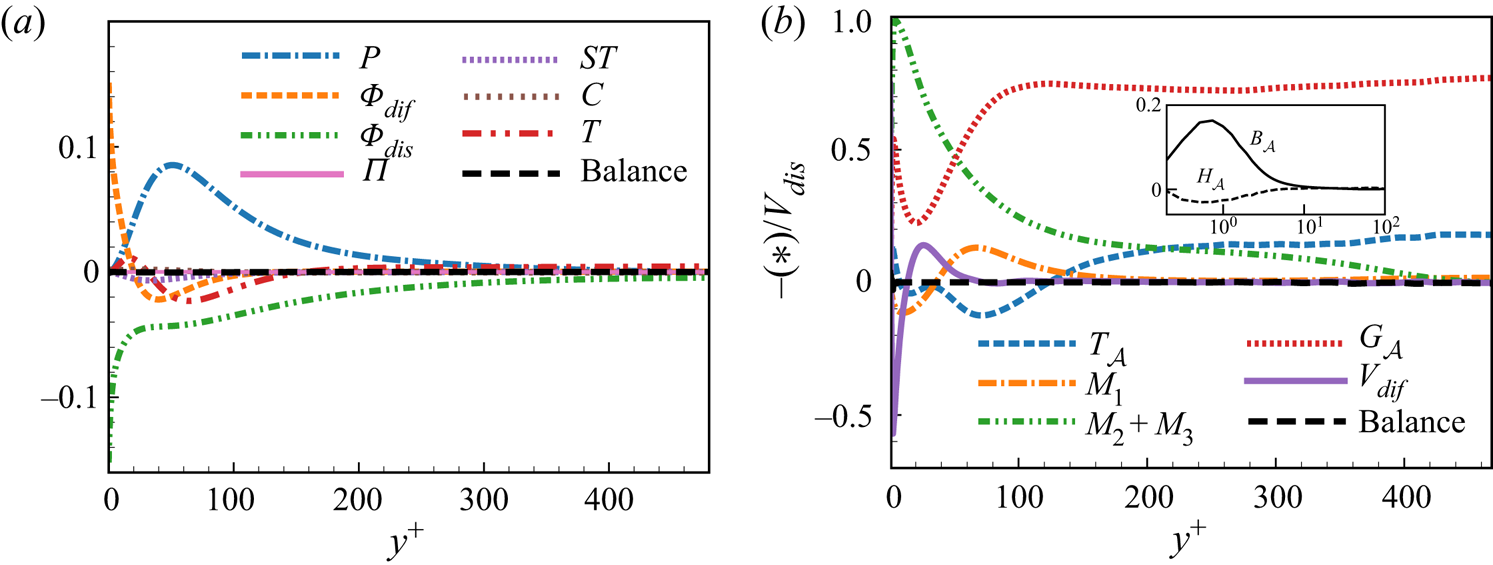
Figure 1(a) shows the vertical distributions of each term of the budget equation of TKE. The results show that the transport of TKE is dominated by the terms  $P$,
 $\varPhi _{dif}$,
 $\varPhi _{dis}$ and
 $T$. The term
 $P$ in the buffer layer leads to the strong generation of TKE, and the term
 $T$ transports TKE from the viscous sublayer to the outer regions. Currently, it is found that the budget of TKE is well balanced, which is also consistent with the previous results for compressible wall turbulence (Foysi, Sarkar & Friedrich Reference Foysi, Sarkar and Friedrich2004; Duan, Beekman & Martín Reference Duan, Beekman and Martín2010).
 $(a)$ The balance of the budget of TKE.
 $(b)$ The equilibrium of the transport equation of the fluctuating VGT's amplitude, non-dimensionalized by the inverse value of the viscous dissipation term.

The VGT is defined as  ${\mathsf{A}}_{ij}=\partial u_i/\partial x_j$, and its fluctuation is
 ${\mathsf{A}}'_{ij}={\mathsf{A}}_{ij}-\overline {{\mathsf{A}}_{ij}}$. To validate the accuracy of the VGT in the database, the amplitude of
 ${\mathsf{A}}'_{ij}$ is defined as
 $\mathcal {A}=\overline {{\mathsf{A}}'_{ij}{\mathsf{A}}'_{ij}}$ and its transport equation is examined. Similar to the incompressible case (Vreman & Kuerten Reference Vreman and Kuerten2014), the transport equation of
 $\mathcal {A}$ in compressible wall turbulence reads
 \begin{align} \frac{\partial\mathcal{A}}{\partial t}&= \underbrace{-\bar{v}\frac{\partial\mathcal{A}}{\partial y}}_{C_{\mathcal{A}}} \underbrace{ -2\overline{v'{\mathsf{A}}'_{ij}}\frac{\partial \overline{{\mathsf{A}}_{ij}}}{\partial y}}_{M_1} \underbrace{ -2\overline{{\mathsf{A}}_{ik}}\,\overline{{\mathsf{A}}'_{kj}{\mathsf{A}}'_{ij}}}_{M_2} \underbrace{ -2\overline{{\mathsf{A}}_{kj}}\,\overline{{\mathsf{A}}'_{ik}{\mathsf{A}}'_{ij}}}_{M_3} \underbrace{-2\overline{{\mathsf{A}}'_{ik}{\mathsf{A}}'_{kj}{\mathsf{A}}'_{ij}}}_{G_{\mathcal{A}}} \nonumber\\ &\quad \underbrace{-2\overline{{\mathsf{A}}'_{ij}{\mathsf{H}}'_{ij}}}_{H_{\mathcal{A}}} +\underbrace{2\frac{\partial}{\partial y}\overline{{\mathsf{A}}'_{iy} \left(\frac{1}{\rho}\frac{\partial \tau_{ik}}{\partial x_k}\right)' }}_{V_{dif}} \underbrace{-2\overline{\left(\frac{1}{\rho}\frac{\partial \tau_{ik}}{\partial x_k}\right)' \frac{\partial {\mathsf{A}}'_{ij}}{\partial x_j}}}_{V_{dis}} \nonumber\\ &\quad \underbrace{-\frac{\partial}{\partial y}\overline{v'{\mathsf{A}}'_{ij}{\mathsf{A}}'_{ij}}}_{T_{\mathcal{A}}} +\underbrace{2\overline{{\mathsf{A}}'_{ij}{\mathsf{B}}'_{ij}}}_{B_{\mathcal{A}}} +\underbrace{\overline{{\mathsf{A}}'_{ij}{\mathsf{A}}'_{ij}\frac{\partial u'_k}{\partial x_k}}}_{D_{\mathcal{A}}}. \end{align}
In the above equation,  $C _\mathcal {A}$ is the convection of
 $\mathcal {A}$ due to the mean flow;
 $M_2$,
 $M_3$ and
 $M_1$ are the generation terms of
 $\mathcal {A}$ caused by the gradient and second-order gradient of mean velocity (these three terms vanish in homogeneous turbulence);
 $G_\mathcal {A}$ is also a generation term connected to the generation of fine scales by vortex stretching;
 $H_\mathcal {A}$ is a pressure-strain type of term;
 $V_{ dif }$ and
 $V_{ dis }$ are viscous diffusion and dissipation terms, respectively;
 $T_\mathcal {A}$ is the turbulent transport term;
 $B_\mathcal {A}$ denotes the baroclinic effect, which can usually be neglected in regions where the Mach number is relatively low or in the region far from shock waves; and
 $D_{ \mathcal {A}}$ is the generation term when the dilatation is non-zero, and it can also be neglected when the compressibility is weak. Figure 1(b) shows the profiles of each term in (2.2) normalized by the negative value of the viscous dissipation term
 $V_{dis}$ with respect to
 $y^+$. The balanced error of
 $\mathcal {A}$ is less than
 $1\,\%$ in most areas of the channel (
 $y^+>3$), which is approximately
 $5\,\%$ due to the large gradient at the position very close to the wall.
As shown in figure 1(b), it is seen that when  $y^+ \gtrsim 140$ the transport of
 $\mathcal {A}$ is balanced by
 $G_\mathcal {A}$,
 $M_2 + M_3$ and
 $T_\mathcal {A}$. The term
 $M_1$ due to the VGT's inhomogeneity only has a small contribution in the range of
 $40 \lesssim y^+ \lesssim 140$. These characteristics are similar to those in incompressible turbulent channel flow (Vreman & Kuerten Reference Vreman and Kuerten2014). However, near the wall, the transport of
 $\mathcal {A}$ in compressible turbulent channel flow is different from that in incompressible turbulence. When
 $y^+ \lesssim 50$, the generation terms
 $M_2 + M_3$ caused by the mean velocity gradient play a leading role, which is much larger than that of
 $G_\mathcal {A}$. However, near the wall in incompressible turbulent channel flow, the terms
 $M_1$,
 $M_2+M_3$ and
 $G_\mathcal {A}$ have similar amplitudes, and the action of viscosity balances the sum of them. This difference may be due to the fact that there are dramatic changes in density and temperature near the wall in the compressible case. Meanwhile, the terms
 ${H}_\mathcal {A}$ and
 $B_\mathcal {A}$ are also shown in figure 1(b), and their amplitudes are quite small. However, it should be emphasized that they play a key role in counteracting the finite-time singularity of the RE equation (Chevillard & Meneveau Reference Chevillard and Meneveau2006; Lüthi et al. Reference Lüthi, Holzner and Tsinober2009; Chevillard et al. Reference Chevillard, Lévêque, Taddia, Meneveau, Yu and Rosales2011; Johnson & Meneveau Reference Johnson and Meneveau2016). Although the term
 ${H}_\mathcal {A}$ almost does not change the amplitude of
 $\mathcal {A}$, it can redistribute the energy of the VGT between components (Vreman & Kuerten Reference Vreman and Kuerten2014). Suman & Girimaji (Reference Suman and Girimaji2013) pointed out that, in compressible isotropic decaying turbulence, the gradient steepening (smoothing) action of pressure is found to be associated with a negative (positive) growth rate of dilatation rate. Therefore, the cancellation effect leads to
 ${H}_\mathcal {A}$ having little impact on
 $\mathcal {A}$. Finally, the term
 $B_\mathcal {A}$ can promote the generation of
 $\mathcal {A}$ near the wall due to the dramatic changes in density and temperature near the wall.
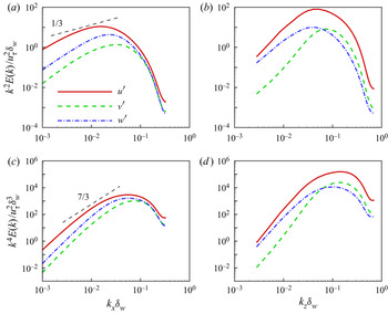
For high-frequency fluctuations, the one-dimensional spectra of the first and second derivatives of fluctuating velocity in the buffer layer are shown in figure 2. Since the spectrum  $E(k)$ of TKE follows the power-law decay of
 $k^{-5/3}$ (Pope Reference Pope2000) in the inertial range, the energy spectrum
 $k^{2n}E(k)$ of the
 $n$th-order derivative of velocity has a power-law decay of
 $k^{2n-5/3}$. For the first-order derivative and second-order derivative of velocity, the exponents of the power-law decay are
 $1/3$ and
 $7/3$, respectively. Figure 2 shows that, in the one-dimensional energy spectrum in the buffer layer at
 $y^+=20.5$, there is a narrow wavenumber range in which the spectra have scaling laws comparable to the standard inertial power law; however, this is a reasonable result as
 $Re_\tau =532$ considered is relatively low. The maximum value of the spectrum is reached in the viscous range and then decays rapidly. The ratio of the peak value of the one-dimensional spectrum to the value of maximum wavenumber is defined as spectral fall-off (Vreman & Kuerten Reference Vreman and Kuerten2014). The fall-offs of one-dimensional spanwise and streamwise energy spectra are over two orders of magnitude, suggesting that the present simulation's resolution is sufficient.
In the buffer layer of  $y^+=20.5$, (a,b) the spectra of first-order velocity derivative, and (c,d) the spectra of second-order velocity derivative. Panels (a,c) and (b,d) illustrate one-dimensional spectra in the streamwise and spanwise directions, respectively. Here
 $u_\tau$,
 $\delta _w$,
 $k_x$ and
 $k_z$ are the friction velocity, the viscous length scale evaluated at the wall and the wavenumbers in the streamwise and spanwise directions, respectively.

3. Evolution equation of the VGT invariants
In this section, some basic concepts and formulae are introduced, including the definitions and physical meanings of the VGT invariants and flow topology, and the evolution equations of invariants with the contributions of pressure-Hessian tensor.
3.1. Invariants and flow topology
The eigenvalues  ${\varLambda }_\alpha$ (
 $\alpha =1, 2, 3$) of the VGT,
 $\boldsymbol{\mathsf{A}}$, are obtained as solutions of the characteristic equation
 \begin{equation} {\varLambda}_\alpha^3+P{\varLambda}_\alpha^2+Q{\varLambda}_\alpha+R=0, \end{equation}
where  $P$,
 $Q$ and
 $R$ are the first, second and third invariants of
 $\boldsymbol{\mathsf{A}}$. The VGT can be split up into the symmetric part
 $ {\mathsf {S}}_{ij}=( {\mathsf {A}}_{ij}+ {\mathsf {A}}_{ji})/2$ and the antisymmetric part
 $ {\mathsf {W}}_{ij}=( {\mathsf {A}}_{ij}- {\mathsf {A}}_{ji})/2$, i.e. the strain-rate tensor
 $\boldsymbol{\mathsf{S}}$ and rotation-rate tensor
 $\boldsymbol{\mathsf{W}}$. Similar to (3.1), the invariants of
 $\boldsymbol{\mathsf{S}}$ and
 $\boldsymbol{\mathsf{W}}$ can be defined and described as
 $P_S$,
 $Q_S$,
 $R_S$ and
 $P_W$,
 $Q_W$,
 $R_W$, respectively. The invariants can be computed from the components of the strain-rate tensor and rotation-rate tensor (see (A1) and (A2)). While
 $P_W$ and
 $R_W$ are zero, the rest of the invariants are connected with each other as
 \begin{equation} P=P_S, \quad Q=Q_S+Q_W, \quad R=R_S+PQ_W-{\mathsf{W}}_{ij}{\mathsf{W}}_{jk}{\mathsf{S}}_{ik}. \end{equation}
Based on the definition of vorticity,  $\boldsymbol { \omega } = \boldsymbol {\nabla } \times \boldsymbol {u}$, we can obtain
 \begin{equation} Q_W=\tfrac{1}{4}\omega_k\omega_k,\quad R=R_S-\tfrac{1}{4}\omega_i{\mathsf{S}}_{ij}\omega_j. \end{equation}
If we define
 \begin{equation} R_\omega=\tfrac{1}{4}\boldsymbol{\omega}\boldsymbol{\cdot} \boldsymbol{\mathsf{S}} \boldsymbol{\cdot}\boldsymbol{\omega}, \end{equation}
which is the vortex stretching to promote enstrophy (Tsinober Reference Tsinober2009), the third invariant  $R$ can be written as
 \begin{equation} R=R_S-R_\omega. \end{equation}
All these invariants have definite physical meanings. First of all, the first invariant,  $P$ or
 $P_S$, is exactly the opposite of dilatation. In incompressible flow, where the dilatation vanishes, the form of the invariants can be simplified. Secondly, if we neglect the variation of viscosity coefficient
 $\nu$, the mechanical energy dissipation rate per unit mass can be expressed as (Chu & Lu Reference Chu and Lu2013)
 \begin{equation} {\varPhi}=2\nu ({\mathsf{S}}_{ij}{\mathsf{S}}_{ij}-\tfrac{1}{3}P^2 ) ={-}4\nu (Q_S-\tfrac{1}{3}P^2 )>0. \end{equation}
Thus,  $Q_S-P^2/3$ is proportional to the dissipation rate of mechanical energy, which is always a negative value. In the region far from the shock wave, the amplitude of dilatation is usually small compared to the strain rate and vorticity, so
 $Q_S$ is also negative and contributes dominantly to dissipation. Additionally,
 $Q_W$ is one-quarter of the enstrophy according to (3.3a,b). As a result, the second invariant
 $Q$ represents the competition between mechanical energy dissipation and enstrophy. Lastly, it will be seen in the following discussion that
 $R_S$ is the generation rate of mechanical energy dissipation due to the nonlinear effect. Thus the third invariant
 $R$ represents the competition between the generation rate of dissipation and the vortex stretching.
The discriminant of the eigenvalue equation (3.1) is
 \begin{equation} \varDelta=27R^2+(4P^3-18PQ)R+(4Q^3-P^2Q^2), \end{equation}
which determines the root properties. When  $\varDelta < 0$, there are three real roots. When
 $\varDelta > 0$, there is a real root and a conjugate pair of complex roots. The discriminant
 $\varDelta = 0$ can be decomposed into two intersecting surfaces
 $r^{(1a)}$ and
 $r^{(1b)}$:
 $$\begin{gather} P(9Q-2P^2)-2({-}3Q+P^2)^{3/2}-27R=0, \end{gather}$$
 $$\begin{gather}P(9Q-2P^2)+2({-}3Q+P^2)^{3/2}-27R=0. \end{gather}$$
When  $\varDelta > 0$, the complex roots on the surface
 $r^{(2)}$,
 $PQ-R=0$, are pure imaginary numbers. According to the critical point theory (Chong et al. Reference Chong, Perry and Cantwell1990), the
 $P$–
 $Q$–
 $R$ spaces can be separated by surfaces
 $r^{(1a)}$,
 $r^{(1b)}$,
 $r^{(2)}$ and
 $R=0$ into regions with different flow topologies.
Generally, the distribution of invariants in the  $P$–
 $Q$–
 $R$ space is very complex and not easy to describe intuitively. Therefore, the distribution and evolution of the flow topology in the
 $Q$–
 $R$ plane can usually be studied for compression, expansion or incompressible regions by fixing the value of
 $P$ (Suman & Girimaji Reference Suman and Girimaji2010; Wang & Lu Reference Wang and Lu2012; Chu & Lu Reference Chu and Lu2013; Bechlars & Sandberg Reference Bechlars and Sandberg2017), respectively. In this case, the interface of flow topologies degenerates to the borderline in the plane
 $Q$–
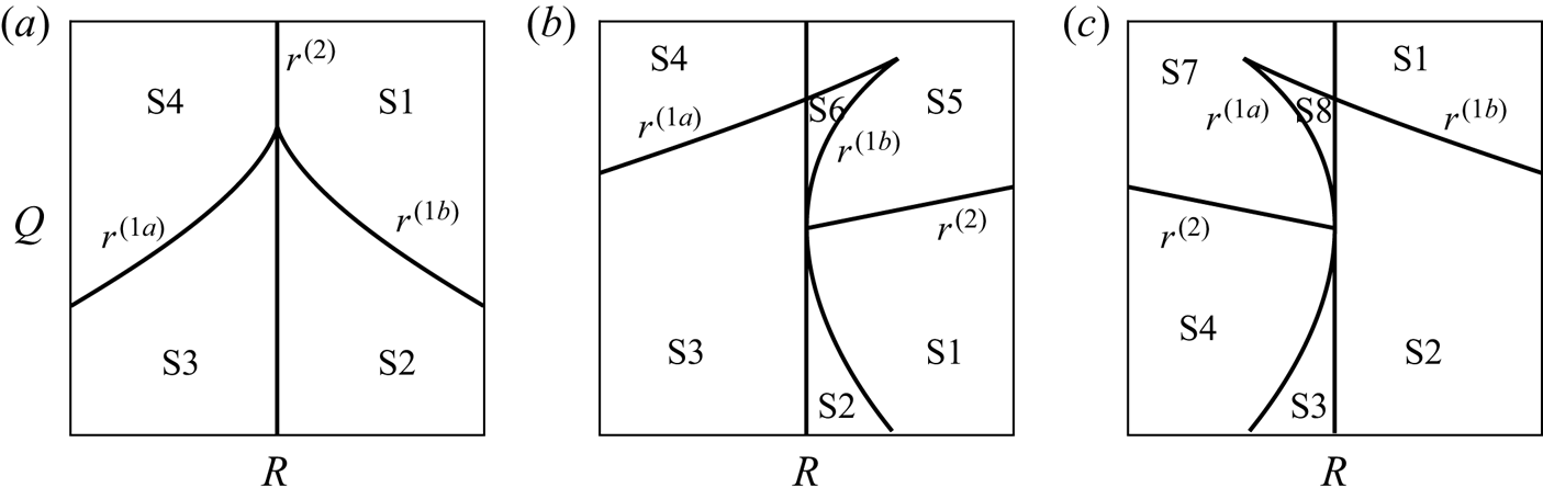
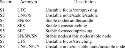
 $R$. Figure 3 shows the classification of flow topologies in the
 $Q$–
 $R$ plane for different dilatation. Table 1 lists the possible flow topologies and their acronym (Suman & Girimaji Reference Suman and Girimaji2010; Wang & Lu Reference Wang and Lu2012; Wang et al. Reference Wang, Wan, Chen, Xie, Zheng, Wang and Chen2020).
The classification of flow topologies in the plane  $Q$–
 $R$ (Wang & Lu Reference Wang and Lu2012): (a)
 $P=0$; (b)
 $P>0$; and (c)
 $P<0$.

Acronyms and descriptions of different flow topologies (Wang & Lu Reference Wang and Lu2012).

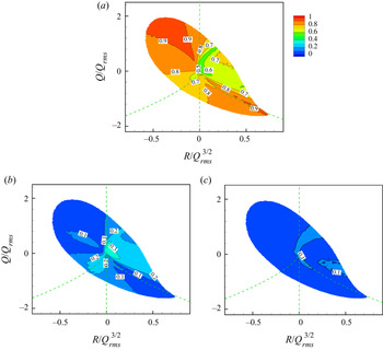
As shown in figure 3(a), when  $P=0$, the borderlines
 $r^{(1a)}$ and
 $r^{(1b)}$ are symmetric with respect to the
 $Q$-axis in the
 $Q$–
 $R$ plane, and
 $r^{(2)}$ coincides with the axis
 $R=0$. There are four kinds of flow topologies in the
 $Q$–
 $R$ plane. When
 $P>0$, the curves
 $r^{(1a)}$ and
 $r^{(1b)}$ are no longer symmetric,
 $r^{(1b)}$ intersects with
 $r^{(2)}$ at
 $(R,Q) = (0,0)$, and there are six flow topologies in the
 $Q$–
 $R$ plane. Similarly, when
 $P<0$,
 $r^{(1a)}$ intersects with
 $r^{(2)}$ at
 $( R,Q) = (0,0)$. Then, the
 $Q$–
 $R$ plane is also split up into six regions, corresponding to six kinds of flow topologies.
3.2. The evolution equation of invariants
Evolution equations of the VGT can be obtained by taking the gradient on both sides of the compressible Navier–Stokes equations (Cantwell Reference Cantwell1993; Martín et al. Reference Martín, Ooi, Chong and Soria1998b; Ooi et al. Reference Ooi, Martin, Soria and Chong1999; Meneveau Reference Meneveau2011; Chu & Lu Reference Chu and Lu2013), expressed as
 \begin{equation} \frac{\mathcal{D}{\mathsf{A}}_{ij}}{\mathcal{D}t} =-{\mathsf{A}}_{ik}{\mathsf{A}}_{kj}-{\mathsf{H}}_{ij}-{\mathsf{B}}_{ij}+{\mathsf{V}}_{ij}, \end{equation}
where  ${\mathcal {D}}/{\mathcal {D}t}=\partial /\partial t+\boldsymbol {u}\boldsymbol {\cdot }\boldsymbol {\nabla }$ stands for the Lagrangian material derivative, the first term on the right-hand side is a nonlinear self-amplification term, and
 \begin{equation} {\mathsf{H}}_{ij}=\frac{1}{\rho}\frac{\partial^2 p}{\partial x_i\partial x_j}, \quad {\mathsf{B}}_{ij}={-}\frac{1}{\rho^2}\frac{\partial p}{\partial x_i} \frac{\partial\rho}{\partial x_j}, \quad {\mathsf{V}}_{ij}=\frac{\partial}{\partial x_j} \left(\frac{1}{\rho}\frac{\partial \tau_{ik}}{\partial x_k}\right), \end{equation}
where  $ {\mathsf {H}}_{ij}$ is the pressure-Hessian tensor,
 $ {\mathsf {B}}_{ij}$ denotes the baroclinic effect and
 $ {\mathsf {V}}_{ij}$ is the viscous effect, respectively. For incompressible flow, the pressure-Hessian tensor is usually decomposed into an isotropic part and a deviatoric part, namely
 \begin{equation} {\mathsf{H}}_{ij}=\frac{\mathrm{tr}(\boldsymbol{\mathsf{H}})}{3}\delta_{ij} + \tilde{{\mathsf{H}}_{ij}}. \end{equation}
According to Poisson's equation of pressure, we can find  $\mathrm {tr}(\boldsymbol{\mathsf{H}})=2Q= {\mathsf {A}}_{ik} {\mathsf {A}}_{ki}$, which means that the isotropic part of
 $ {\mathsf {H}}_{ij}$ is explicitly related with
 $ {\mathsf {A}}_{ij}$ and its contribution is equivalent to the nonlinear self-amplification term. Thus, it can be absorbed in the nonlinear term (Meneveau Reference Meneveau2011). In this study, the flow compressibility is relatively weak, so the isotropic part of
 $ {\mathsf {H}}_{ij}$ is also absorbed in the nonlinear term. Only the contribution of the pressure-Hessian tensor's deviatoric part to the VGT dynamics is considered here. The baroclinic effect is ignored due to the weak compressibility.
Following the works of Chu & Lu (Reference Chu and Lu2013) and Bechlars & Sandberg (Reference Bechlars and Sandberg2017), the evolution equations of the invariants ( $Q,\ Q_S,\ Q_W,\ R,\ R_S$) and
 $R_\omega$ can be obtained from their definitions and the dynamic equation (3.9) of the VGT (see Appendix A for details). The physical meaning of
 $R_S$ can be revealed by the evolution equation (A3) of
 $Q_S$. The nonlinear generation term of
 $Q_S$, i.e.
 $Q_SS$, can be evaluated as
 \begin{equation} Q_SS={-}3R_S +R_\omega +P(Q_S-Q_W) +\tfrac{2}{3}P\,\mathrm{tr}(\boldsymbol{\mathsf{H}}). \end{equation}
This generation term is composed of the third invariant ( $R_S$) of the strain-rate tensor, a vortex-stretching term and a dilatation-related term. In turbulence studies, it has been found that the vortex-stretching behaviour always tends to increase enstrophy (Pope Reference Pope2000; Tsinober Reference Tsinober2009). Therefore, when the compressibility is small, the generation of
 $Q_S$ is mainly determined by the competition between
 $R_\omega$ and
 $-3R_S$. Since
 $Q_S$ is roughly proportional to the opposite number of mechanical energy dissipation, the physical meaning of
 $R_S$ is the nonlinear generation rate of mechanical energy dissipation.
The evolution equations (A3)–(A5) and (A7)–(A9) describe the evolution of invariants involving dissipation, enstrophy and their mutual competition, and the dynamic equations of the three generation mechanisms, which mainly include the nonlinear generation term and pressure-Hessian term, baroclinic term and viscous term, of which the pressure-Hessian term is the focus of this study.
3.3. The pressure-Hessian tensor in the principal coordinate system
The dynamics of the vorticity and the strain-rate tensor are generally studied under a fixed reference frame. However, She, Jackson & Orszag (Reference She, Jackson and Orszag1991) provided further insight into this dynamical system by examining their dynamics in the principal coordinate system of the strain-rate tensor. Let the eigenvectors of the strain-rate tensor  $\boldsymbol{\mathsf{S}}$ be
 $\boldsymbol {e}_1$,
 $\boldsymbol {e}_2$ and
 $\boldsymbol {e}_3$, and the corresponding eigenvalues be
 $\lambda _1 \geq \lambda _2 \geq \lambda _3$. In this principal coordinate system of the local strain-rate tensor, the contribution components of the pressure-Hessian term (neglecting the dilatation-related terms) to the invariants
 $Q$,
 $Q_S$ and
 $R_S$ (see (A3), (A5) and (A7)) can be written as
 $$\begin{gather} QH=Q_SH= \boldsymbol{\mathsf{S}} \boldsymbol{:} \tilde{\boldsymbol{\mathsf{H}}}= \lambda_1 \hat{{\mathsf{H}}}_{11}+\lambda_2 \hat{{\mathsf{H}}}_{22}+ \lambda_3 \hat{{\mathsf{H}}}_{33}, \end{gather}$$
 $$\begin{gather}R_S H= \boldsymbol{\mathsf{S}}^2 \boldsymbol{:} \tilde{\boldsymbol{\mathsf{H}}}= \lambda_1^2 \hat{{\mathsf{H}}}_{11}+\lambda_2^2 \hat{{\mathsf{H}}}_{22}+ \lambda_3^2 \hat{{\mathsf{H}}}_{33}, \end{gather}$$
where  $\hat {(\cdot )}$ represents the tensorial component in the principal coordinate system. Thus, the effect of the pressure-Hessian tensor on the dynamic evolution of
 $Q$ (or
 $Q_S$) and
 $R_S$ includes the sum of its generation effects on the three principal strain rates (i.e.
 $\lambda _1,\ \lambda _2$ and
 $\lambda _3$), respectively.
On the other hand, suppose that the eigenvalues including the isotropic part of  $\boldsymbol{\mathsf{H}}$ are
 $|\varpi _1| \geq | \varpi _2 | \geq | \varpi _3 |$, with the corresponding principal directions
 $\boldsymbol {f }_1$,
 $\boldsymbol {f}_2$ and
 $\boldsymbol {f}_3$, which are also the principal directions of the deviatoric part of
 $\tilde {\boldsymbol{\mathsf{H}}}$. The eigenvalues of
 $\tilde {\boldsymbol{\mathsf{H}}}$ are assumed to be
 $\eta _1$,
 $\eta _2$ and
 $\eta _3$, which correspond to
 $\varpi _1$,
 $\varpi _2$ and
 $\varpi _3$, respectively. The contribution of the pressure-Hessian tensor to
 $R_\omega$ shown in (A8) can be expressed as
 \begin{align} R_\omega H={-}\tfrac{1}{4}\boldsymbol{\omega}\boldsymbol{\cdot} \tilde{\boldsymbol{\mathsf{H}}}\boldsymbol{\cdot}\boldsymbol{\omega}={-}\tfrac{1}{4}\omega^2[\eta_1\cos^2 (\,\boldsymbol{f}_1,\boldsymbol{\omega})+ \eta_2\cos^2 (\,\boldsymbol{f}_2,\boldsymbol{\omega})+ \eta_3\cos^2 (\,\boldsymbol{f}_3,\boldsymbol{\omega})], \end{align}
which contains the three eigenvalues and the cosine of relative angles between the principal directions and the vorticity. From (A13), the stretching of the pressure-Hessian tensor on vorticity should be understood as a phenomenon observed in the rotating coordinate system, and the essence is that the pressure-Hessian tensor affects vorticity by changing the coordinates in the principal coordinate system.
Based on the decomposition shown in (3.13)–(3.15), the effect of the pressure-Hessian tensor on the dynamic evolution of invariants and vortex stretching can be simplified and interpreted as the sum of its generation effects on the three principal strain rates, respectively. This motivates a term-by-term investigation on the pressure-Hessian's contribution associated with each principal strain rate. Thus we will study the geometrical relationships between the pressure-Hessian tensor and the vorticity/strain-rate tensor. Then, the direct contributions of the pressure-Hessian tensor to the dynamics of  $Q_S$,
 $R_S$ and
 $R_\omega$ will be investigated.
4. Results and discussion
In this section, we first discuss the joint probability density function (p.d.f.) of invariants and the probability of flow topology in a weakly compressible turbulent channel flow, and then analyse the structural characteristics of the pressure-Hessian tensor in different topological regions, focusing on its relationship with the vorticity and the strain-rate tensor. On the aforementioned basis, we further discuss the contribution of the pressure-Hessian tensor to the dynamical evolution of invariants. Finally, the modelling implications for VGT dynamics based on the present findings are discussed.
4.1. Joint p.d.f. of invariants and the volume fraction of flow topologies
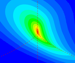
Figure 4(a) shows the joint p.d.f. of invariants  $Q$ and
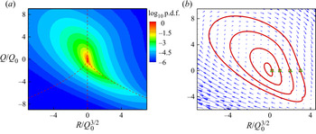
 $R$ for the whole channel. Since the compressibility is relatively weak in the present case, the change of dilatation has not been considered here. It is seen that the contours of the joint p.d.f. of invariants present a self-similar ‘tear-drop’ shape, which is consistent with the previous results for different types of turbulence (Ooi et al. Reference Ooi, Martin, Soria and Chong1999; Tsinober Reference Tsinober2009; Meneveau Reference Meneveau2011). To study the invariants’ dynamic evolution, Martín et al. (Reference Martín, Ooi, Chong and Soria1998b) adopted the CMT in the space of
 $Q$–
 $R$ to describe the mean Lagrangian evolution of the invariants. Here, we also calculate the conditional mean of the material derivative of the invariant, and regard it as the conditional mean velocity of the invariant in the
 $Q$–
 $R$ plane:
 \begin{equation} \boldsymbol{v}=(v_R,v_Q) =\left\langle\left.\left(\frac{\mathcal{D}R}{\mathcal{D}t}, \frac{\mathcal{D}Q}{\mathcal{D}t}\right)\right\vert (R,Q )\right\rangle. \end{equation}
By integrating  $\boldsymbol {v}$, the CMT of the invariant can be obtained.
(a) The log scale of joint p.d.f. of invariants  $Q$ and
 $R$ for the whole channel. (b) The CMTs of
 $Q$ and
 $R$, with the start points
 $(0.25,0),\ (1,0),\ (2,0)$ and
 $(3,0)$ denoted by square symbols and the end points denoted by triangular symbols. The vectors represent the conditional mean velocity
 $\boldsymbol {v}$ of invariants. Here
 $Q$ and
 $R$ are normalized by
 $Q_0=\int _{-h}^{h} Q_{rms}(y)\,\mathrm {d}y/2h$.

From the perspective of probability conservation, Lozano-Durán et al. (Reference Lozano-Durán, Holzner and Jiménez2015) and Lozano-Durán, Holzner & Jiménez (Reference Lozano-Durán, Holzner and Jiménez2016) claimed that the CMT must be a closed curve for the flow in a statistical steady and homogeneous turbulence or in a periodic domain, and the closure behaviour of the trajectory is significantly affected by the numerical accuracy. Figure 4(b) shows the conditional mean trajectories of the invariants for the whole channel. Four trajectories that start from four different positions on the axis  $Q=0$ and arrive at positions near their start positions after a clockwise circle are shown, which form closed curves, suggesting that the present calculation's numerical accuracy is sufficient.
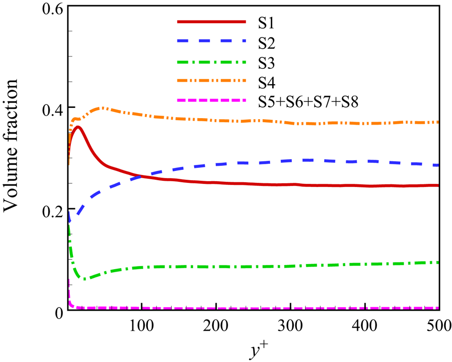
To understand the probability of different flow topologies arising in the channel, the volume fraction distribution of different flow topologies along the wall-normal direction ( $y^+$) is shown in figure 5. It is found that when
 $y^+\gtrsim 150$ the proportion of flow topologies varies little with
 $y^+$, which is similar to the statistical results of homogeneous isotropic turbulence (Suman & Girimaji Reference Suman and Girimaji2010). In the inner layer of
 $y^+ \lesssim 150$, the proportion of different flow topologies varies significantly due to the increase of mean shear (Wang & Lu Reference Wang and Lu2012). The flow topology S4 has the largest volume fraction in the whole channel since the flow field is full of vortices. When
 $y^+ \gtrsim 100$, except for S4, the proportions of S2, S1 and S3 are also relatively high and decrease in turn. When
 $y^+ \lesssim 100$, with the decrease of
 $y^+$, the ratio of unstable focus and compressed topology S1 increases to the same probability as S4, and the probability of S2 decreases to the same probability as S3. The volume fraction of the flow topologies S5–S8 due to compressibility is also very low, which can be neglected in all other regions except very close to the wall. As a result, in the following discussions, these flow topologies (i.e. S5–S8) will be ignored. In contrast, the effects of the flow topologies S1–S4 on the statistical properties of the pressure-Hessian tensor will be discussed in detail.
The distribution of volume fraction of different flow topologies versus  $y^+$.

4.2. The geometrical relationships between the pressure-Hessian tensor and the vorticity/strain-rate tensor
Since the vorticity and strain rate are represented by the antisymmetric part and symmetric part of the VGT, understanding the geometrical relationship between the vorticity and the pressure-Hessian tensor is of great significance to explore the non-local effect of the pressure-Hessian tensor on the dynamics of the VGT (Suman & Girimaji Reference Suman and Girimaji2013). The analysis of incompressible isotropic turbulence reveals that the vorticity tends not only to be parallel to the second principal direction of the strain-rate tensor ( $\boldsymbol {e}_2$) but also to be parallel to the second principal direction of the pressure-Hessian tensor. The first and third principal directions of the pressure-Hessian tensor tend to be in the plane
 $\boldsymbol {e}_1$–
 $\boldsymbol {e}_3$, and the preferential relative angles with
 $\boldsymbol {e}_1$ and
 $\boldsymbol {e}_3$ are about
 ${\rm \pi} /4$ (Ohkitani Reference Ohkitani1993; Kalelkar Reference Kalelkar2006). Here, the second principal direction corresponds to the second eigenvector when the eigenvalues are ordered in descending order, rather than the principal direction
 $\boldsymbol {f}_2$ defined in this study. These findings have also been confirmed to be valid in compressible isotropic decaying turbulence. Lawson & Dawson (Reference Lawson and Dawson2015) found that if the eigenvalues of the pressure-Hessian tensor (including the isotropic part) were sorted by their absolute values, the third principal direction appears to be aligned with the vorticity in the rotation-dominated regions (i.e.
 $Q>0$). In the strain-dominated regions, the third principal direction tends to be parallel to
 $\boldsymbol {e}_2$. Next, we will present the alignment statistics of the pressure-Hessian tensor with the strain-rate tensor/vorticity in the present wall turbulence, and the influence of different flow topologies is also considered.
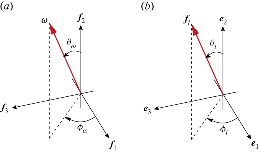
To describe the vectors’ geometrical relationship, the azimuthal angle  $\phi$ and polar angle
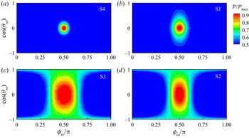
 $\theta$ are defined (Zamansky, Vinkovic & Gorokhovski Reference Zamansky, Vinkovic and Gorokhovski2011; Lawson & Dawson Reference Lawson and Dawson2015), as illustrated in figure 6. Figure 7 shows the statistical results of the joint p.d.f.
 $\mathcal {P}(\theta _\omega, \phi _\omega )/\mathcal {P}_{max}$ of the vorticity in the central plane of the channel (
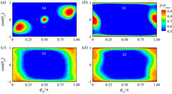
 $y^+=532$) for the flow topologies S1–S4. As shown in figure 7(a,b), the statistical properties are generally similar to those of incompressible isotropic turbulence (Lawson & Dawson Reference Lawson and Dawson2015). In the S1 and S4 flow topologies with focus, the maximum value of p.d.f. in the plane
 $\theta _\omega$–
 $\phi _\omega$ occurs near
 $({\rm \pi} /2,{\rm \pi} /2)$. The vorticity is perpendicular to
 $\boldsymbol { f}_1$,
 $\boldsymbol {f}_2$, and aligned with
 $\boldsymbol {f}_3$. In the regions of flow topology S2, the large values of p.d.f. are relatively concentrated near
 $\phi _\omega ={\rm \pi} /2$, indicating that the vorticity is preferentially perpendicular to
 $\boldsymbol {f}_1$. The values of p.d.f. in the range of
 $\theta _\omega \in [-{\rm \pi} /2,{\rm \pi} /2]$ around
 $\phi _\omega ={\rm \pi} /2$ are relatively large, suggesting that the possible direction of the vorticity is distributed in the plane
 $\boldsymbol {f}_2$–
 $\boldsymbol { f}_3$. In the regions of flow topology S3, the p.d.f. has a similar distribution to that of S2, but the distribution is wider, centred at
 $\phi _\omega ={\rm \pi} /2$. These results show that in the channel's central regions, the flow has similar statistical properties to those of isotropic turbulence. The geometrical relationships between the vorticity and the principal directions of the pressure-Hessian tensor show similar properties in the strain-dominated regions and the rotation-dominated regions, regardless of whether the topologies belong to the stable topology or the unstable topology.
(a) The polar angle  $\theta _\omega$ and the azimuthal angle
 $\phi _\omega$ of the vorticity in the principal coordinate system of the pressure-Hessian tensor. (b) The polar angle
 $\theta _i$ and the azimuthal angle
 $\phi _i$ of
 $\boldsymbol {f}_i$ in the principal coordinate system of the strain-rate tensor. Since the orientation of the principal direction can differ by a negative sign, when
 $\phi _\omega <0$, the value can be set as
 $\phi _\omega +{\rm \pi}$. This point is the same for
 $\phi _i$.

The joint p.d.f.  $\mathcal {P}(\theta _\omega, \phi _\omega )/\mathcal {P}_{max}$ of the vorticity in the central plane of the channel (
 $y^+=532$) for different flow topologies: (a) S4, (b) S1, (c) S3 and (d) S2.

Figure 8 shows the joint p.d.f.  $\mathcal {P}(\theta _\omega, \phi _\omega )/\mathcal {P}_{max}$ of the vorticity in the horizontal plane inside the buffer layer of
 $y^+=20.5$ for different flow topologies. It is seen that in the regions of flow topology S4, there are three pairs of angles with peak p.d.f. values, which are roughly
 $(\theta _\omega, \phi _\omega ) = ( {\rm \pi}/2, {\rm \pi}/2 )$,
 $(2{\rm \pi} /3, {\rm \pi}/8)$ and
 $({\rm \pi} /3,7{\rm \pi} /8)$. The pair
 $({\rm \pi} /2, {\rm \pi}/2)$ means that the vorticity is aligned with
 $\boldsymbol {f}_3$, the same as that in the central plane of the channel. Furthermore, by analysing the statistical results of more near-wall positions, it is found that, with the decrease of wall distance, the angle
 $\phi _\omega$ corresponding to the peak p.d.f. value gradually shifts from
 $\phi _\omega ={\rm \pi} /2$ to
 $\phi _{\omega } = 0$ or
 ${\rm \pi}$, and finally
 $(\theta _\omega, \phi _\omega )$ of the peak p.d.f. value reaches
 $({\rm \pi} /2,0 )$ or
 $( {\rm \pi}/2, {\rm \pi})$ in the viscous sublayer. This result shows that when approaching the wall, the vorticity gradually changes from being parallel to
 $\boldsymbol {f}_3$ to being aligned with
 $\boldsymbol {f}_1$ due to the effect of strong mean shear.
(a) The joint p.d.f.  $\mathcal {P}(\theta _\omega, \phi _\omega )/\mathcal {P}_{max}$ of the vorticity in the buffer layer (
 $y^+=20.5$) for different flow topologies: (a) S4, (b) S1, (c) S3 and (d) S2.

Meanwhile, in the regions of flow topology S1, the large p.d.f. values occur near  $(\theta _\omega, \phi _\omega ) = ( {\rm \pi}/2,0)$,
 $({\rm \pi} /2, {\rm \pi})$ and
 $(0,0 \sim {\rm \pi})$ or
 $({\rm \pi}, 0 \sim {\rm \pi})$, that is, the vorticity is aligned with
 $\boldsymbol {f}_1$ or
 $\boldsymbol {f}_2$. The vorticity in the viscous sublayer (S1 region) is ultimately aligned with
 $\boldsymbol {f}_1$. Figure 8(c,d) shows that in the strain-dominated regions, i.e. the regions of flow topology S2 and S3, the distributions of joint p.d.f. are similar, the p.d.f. has a large value as
 $\phi _\omega =0,{\rm \pi}$ and
 $\theta _\omega =0,{\rm \pi}$, suggesting that the most possible direction of the vorticity lies in the plane
 $\boldsymbol {f}_1$–
 $\boldsymbol {f}_2$.
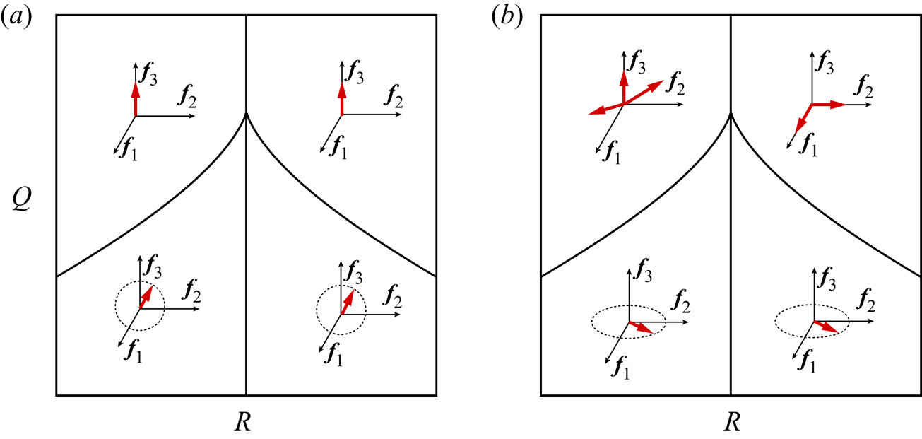
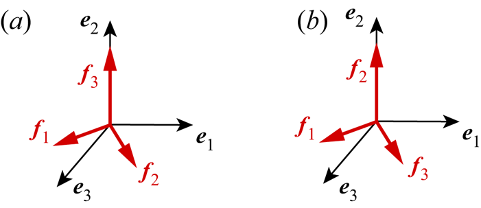
Figure 9 shows the most possible distribution sketch maps of the vorticity direction in the turbulent central regions and buffer layers in the principal coordinate system of the pressure-Hessian tensor. The above results show that in wall turbulence, the geometrical relationship between the vorticity and the pressure-Hessian tensor changes significantly near the wall due to mean shear, implying that the pressure-Hessian tensor is strongly affected by inhomogeneity and anisotropy. Based on (3.15), it is known that the change of the geometrical relationship will directly affect the contribution of the pressure-Hessian tensor to the generation of  $R_\omega$.
The most possible distribution sketch maps of the vorticity direction in the principal coordinate system of the pressure-Hessian tensor for different flow topologies at different vertical positions: (a)  $y^+=532$ and (b)
 $y^+=20.5$. The thick red line with arrowhead indicates the vorticity direction, and the fine lines with arrows are the principal directions of the pressure-Hessian tensor.

Next, we analyse the distribution characteristics of the eigenvalues of the pressure-Hessian tensor. We arrange the eigenvalues  $\eta _1$,
 $\eta _2$ and
 $\eta _3$ of
 $\tilde {\boldsymbol{\mathsf{H}}}$ in descending order, and mark them as
 $\eta _1'\geq \eta _2'\geq \eta _3 '$, and define the normalized eigenvalues as
 \begin{equation} \eta_i^*=\frac{\eta_i'}{\sqrt{\eta_1'^2+\eta_2'^2+\eta_3'^2}}. \end{equation}
Since the trace of  $\tilde {\boldsymbol{\mathsf{H}}}$ is zero, i.e.
 $\eta _1'+\eta _2'+\eta _3'=0$, then the
 $\eta _i^*$ must lie in the ranges
 \begin{equation} \eta_1^*\in[\sqrt{6}/6,\sqrt{6}/3],\quad \eta_2^*\in[-\sqrt{6}/6,\sqrt{6}/6],\quad \eta_3^*\in[-\sqrt{6}/3,-\sqrt{6}/6]. \end{equation}
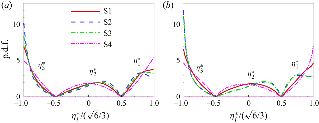
Figure 10 shows the p.d.f. of normalized eigenvalues of the pressure-Hessian tensor. As shown in figure 10(a), in the central region of the channel, different flow topologies have a certain impact on the p.d.f. of eigenvalues. In the S1 and S4 flow topological regions, the maximum values of p.d.f. for  $\eta _1^*$ and
 $\eta _3^*$ are
 $\eta _1^*=\sqrt {6}/3$ and
 $\eta _3^*=-\sqrt {6 }/3$, while in the S4 flow topological regions,
 $\eta _2^*$ reaches the peak value of p.d.f. near zero, and the peak value of p.d.f. for S1 topology corresponds to a positive
 $\eta _2^*$. Since the flow topology S4 is closely related to the vortex structure, it appears that the pressure-Hessian tensor tends to have the first and third eigenvalues with equal absolute value and the second eigenvalue with a value close to zero in the vortical regions. In the regions of strain-dominated flow topology, when the p.d.f. values reach their peaks, the preferred ratio of the corresponding eigenvalues is about
 $\eta _1^*:\eta _2^*:\eta _3^*=-5:1:4$. From figure 10(a,b), it can be found that there is no significant change in the p.d.f.s of the eigenvalues in the central plane and the buffer layer, which means that the eigenvalues of the pressure-Hessian tensor are not sensitive to the mean shear.
The p.d.f. of normalized eigenvalues of the pressure-Hessian tensor at different positions: (a) the central plane,  $y^+=532$, and (b) the buffer layer,
 $y^+=20.5$.

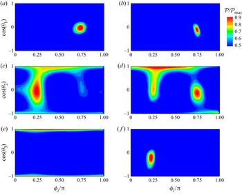
To analyse the geometrical relationship between the pressure-Hessian tensor and the strain-rate tensor, figure 11 shows the joint p.d.f.  $\mathcal {P}(\theta _i,\phi _i)/\mathcal {P}_{max}$ of the polar and azimuthal angles of
 $\boldsymbol {f}_i$ in the principal coordinate system of the strain-rate tensor in the central channel region and the buffer layer. Since the strain rate generally has a large value in the strain-dominated region, only the statistical properties in the S2 and S3 topological regions are considered here. Figure 11(a,c,e) shows that in the central region of the channel, the most preferred angles of
 $\boldsymbol {f}_1$ are
 $( \theta _1, \phi _1 ) = ( {\rm \pi}/2,3{\rm \pi} / 4)$, and the most preferred angles of
 $\boldsymbol {f}_2$ are
 $(\theta _2,\phi _2)=(0,0 - {\rm \pi} )$ or
 $({\rm \pi},0 - {\rm \pi} )$. In short, as shown in the figure 12(a),
 $\boldsymbol {f}_3$ is aligned with
 $\boldsymbol {e}_2$ in the central region of the channel,
 $\boldsymbol {f}_1$ and
 $\boldsymbol {f}_2$ lie in the plane
 $\boldsymbol {e}_1$–
 $\boldsymbol {e}_3$ and the preferred angle with
 $\boldsymbol {e}_1$ is
 ${\rm \pi} /4$, which is consistent with the finding in isotropic turbulence (Lawson & Dawson Reference Lawson and Dawson2015).
The joint p.d.f. of the polar and azimuthal angles,  $\mathcal {P}(\theta _i,\phi _i)/\mathcal {P}_{max}$, for
 $\boldsymbol {f}_i$ in the principal coordinate system of the strain-rate tensor in the strain-dominated regions. Panels (a,b), (c,d) and (e, f) correspond to
 $\boldsymbol {f}_1$,
 $\boldsymbol {f}_2$ and
 $\boldsymbol {f}_3$, respectively; (a,c,e) show the central statistics at
 $y^+=532$ and (b,d, f) show the buffer layer statistics at
 $y^+=20.5$.

Schematic diagrams of the geometrical relationships between  $\boldsymbol {f}_i$ and
 $\boldsymbol {e}_i$ for S2 and S3 topological regions at different wall-normal positions: (a)
 $y^+=532$ and (b)
 $y^+=20.5$.

Figure 11(b,d, f) illustrates that, in the buffer layer, the preferred angles of  $\boldsymbol {f}_1$ in the buffer layer are
 $(\theta _1,\phi _1)=({\rm \pi} /2,3{\rm \pi} /4)$, and the preferred angles of
 $\boldsymbol {f}_3$ are
 $(\theta _3,\phi _3)=({\rm \pi} /2,{\rm \pi} /4)$. The eigenvector
 $\boldsymbol {f}_2$ has multiple preferred directions, e.g.
 $(\theta _2,\phi _2)=(0,0 - {\rm \pi} )$,
 $({\rm \pi} /2,{\rm \pi} /4)$ and
 $({\rm \pi} /2,3{\rm \pi} /4)$. In short, the geometrical relationship between
 $\boldsymbol {f}$ and
 $\boldsymbol {e}$ is illustrated in figure 12(b), i.e.
 $\boldsymbol {f}_2$ is aligned with
 $\boldsymbol {e}_2$,
 $\boldsymbol {f}_1$ and
 $\boldsymbol {f}_3$ lie in the plane
 $\boldsymbol {e}_1$–
 $\boldsymbol {e}_3$ and the preferred angle with
 $\boldsymbol {e}_1$ is
 ${\rm \pi} /4$.
These geometrical relationships between the pressure-Hessian tensor and the vorticity/strain-rate tensor have an apparent statistical propensity, as seen by the above results. With the decrease of wall distance  $y^+$, these geometrical relationships present near-wall statistical properties close to the wall that are significantly different from those in isotropic turbulence. This will be directly related to the pressure-Hessian tensor's contribution to the evolution of the invariant dynamics, which will be further analysed in the following subsection.
4.3. The effects of pressure-Hessian tensor on mean transport of invariants
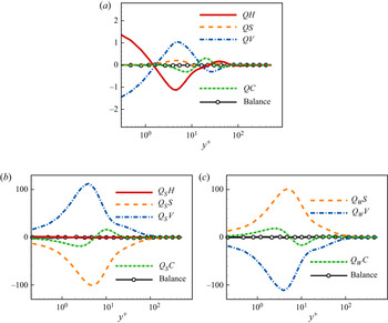
Firstly, the mean transport equations of each invariant are investigated to understand better the dominant balance mechanisms, especially the role of the pressure-Hessian term. Figure 13 shows the wall-normal profiles of the contribution terms in (A3)–(A5) for  $Q$,
 $Q_S$ and
 $Q_W$. When
 $y^+\lesssim 100$, the transport equation of
 $Q$ is mainly balanced by the pressure-Hessian term
 $QH$, the viscosity term
 $QV$ and the convection term
 $QC$, while the contribution of nonlinear term
 $QS$ is relatively small. The transport equation of the opposite value of mechanical energy dissipation
 $Q_S$ is dominated by the viscous term
 $Q_S V$, nonlinear term
 $Q_SS$ and convection term
 $Q_SC$, but the contribution of the pressure-Hessian term
 $Q_SH$ is close to zero. The transport equation of enstrophy
 $Q_W$ is balanced by the generation term
 $Q_W S$, the dissipation term
 $Q_W V$ and the convection term
 $Q_W C$, which does not directly contain the contribution of the pressure-Hessian term. The above phenomena are generally consistent with the statistical properties in other wall turbulence (Balint, Wallace & Vukoslavčević Reference Balint, Wallace and Vukoslavčević1991; Pirozzoli & Grasso Reference Pirozzoli and Grasso2004; Chu et al. Reference Chu, Wang and Lu2014). By partial integration, the contribution of the pressure-Hessian term to the evolution of dissipation can be expressed as (Tsinober Reference Tsinober2009)
 \begin{equation} Q_S H =QH={-}\frac{1}{\rho}\left[ \frac{\partial}{\partial x_i}\left({\mathsf{S}}_{ik}\frac{\partial p}{\partial x_k} -p\frac{\partial {\mathsf{S}}_{ki}}{\partial x_k} \right) +p\frac{\partial^2 P}{\partial x_k\partial x_k}\right] -\frac{1}{3}P{\mathsf{H}}_{kk}. \end{equation}
When the flow is homogeneous and incompressible (i.e.  $P=0$ and the density is constant), then
 $\overline {Q_SH}= 0$. In other words, for the incompressible homogeneous flow, the mean contribution of the pressure-Hessian term to the generation of dissipation should be strictly zero. However, due to inhomogeneity and the small but non-zero compressibility, this mean contribution is not zero in the current turbulence, as seen in the wall-normal profile of
 $QH$. On average, the pressure-Hessian term has a significant contribution to the transport of different components of the VGT, i.e. it mainly redistributes the energy of the VGT between various components (Vreman & Kuerten Reference Vreman and Kuerten2014; Gerolymos & Vallet Reference Gerolymos and Vallet2016).


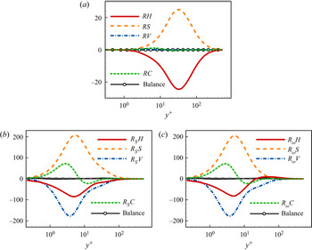
Figure 14 shows the profiles of each term in the mean transport equations of the third invariants ( $R$,
 $R_S$) and
 $R_\omega$ versus
 $y^+$. It is seen that the transport of
 $R$ is balanced by the nonlinear generation term
 $RS$ and the pressure-Hessian term
 $RH$. When
 $y^+\lesssim 100$, the pressure-Hessian term
 $R_SH$, viscous term
 $R_SV$, nonlinear generation term
 $R_SS$ and convection term
 $R_SC$ are the dominant terms in the transport equation of
 $R_S$. On average, the pressure-Hessian term
 $R_SH$ has a negative contribution to the generation of
 $R_S$, the same as the viscous term
 $R_SV$. A similar balance mechanism is also found in the central region of the channel. For the transport of
 $R_\omega$ in the buffer layer and viscous sublayer (
 $y^+ \lesssim 30$), the dominant balance mechanism is the same as that of
 $R_S$, with the pressure-Hessian term showing a negative contribution and weakening
 $R_\omega$. In the outer layer (
 $y^+\gtrsim 30$), the mean effect of the pressure-Hessian term is positive, which is balanced by the sum of the viscous and nonlinear generation terms.


4.4. The decomposition of pressure-Hessian effect
Owing to the strong intermittence of enstrophy, dissipation and their generation processes (Tsinober Reference Tsinober2009), statistical averaging may cover up the real physical insights and thus cannot reflect the turbulent dynamic process. Based on the pressure-Hessian decomposition equations (3.13)–(3.15), the detailed contribution of different components and flow topologies to the dynamic processes of invariants is further discussed. To compare the relative magnitudes of the terms in (3.13)–(3.15), we define
 $$\begin{gather} \varphi_{Q_SH}=\frac{-Q_SH}{\sum_k|\lambda_k\hat{{\mathsf{H}}}_{kk}|},\quad \varphi_{i;Q_SH}=\frac{-\lambda_i\hat{{\mathsf{H}}}_{ii}}{\sum_k|\lambda_k\hat{{\mathsf{H}}}_{kk}|}, \end{gather}$$
 $$\begin{gather}\varphi_{R_SH}=\frac{R_SH}{\sum_k|\lambda^2_k\hat{{\mathsf{H}}}_{kk}|},\quad \varphi_{i;R_SH}=\frac{\lambda^2_i\hat{{\mathsf{H}}}_{ii}}{\sum_k|\lambda^2_k\hat{{\mathsf{H}}}_{kk}|}, \end{gather}$$
 $$\begin{gather}\varphi_{R_\omega H}=\frac{4 R_\omega H/\omega^2}{\sum_k| \eta_k\cos^2 (\boldsymbol{f}_k,\boldsymbol{\omega}) |},\quad \varphi_{i;R_\omega H}=\frac{-\eta_i\cos^2 (\boldsymbol{f}_i,\boldsymbol{\omega})} {\sum_k|\eta_k\cos^2 (\boldsymbol{f}_k,\boldsymbol{\omega})|}, \end{gather}$$
which reflect the relative proportions of the various terms of the pressure-Hessian term.
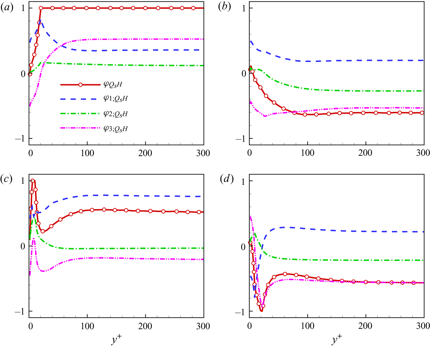
The effect of the pressure-Hessian tensor on the transport of  $Q_S$ can be represented by
 $Q_SH$, and figure 15 shows the profiles of
 $\varphi _{Q_SH}$ and its components versus
 $y^+$. When
 $y^+\gtrsim 100$, the components
 $\varphi _{i;Q_SH}$ basically vary little with
 $y^+$. In the buffer layer and the viscous sublayer, the
 $\varphi _{i;Q_SH}$ change significantly, indicating that the mean shear leads to changes in the action mechanism of the pressure-Hessian term on
 $Q_S$. The term
 $Q_SH$ is dominated by different mechanisms in different flow topologies. As shown in figure 15(a), for the S4 topology, the pressure-Hessian tensor can promote all three principal strain rates in the central region of the channel, increase the amplitude of the strain rate and enhance the dissipation, and the contribution to the third principal strain rate is dominant. With the decrease of
 $y^+$, the contribution of the pressure-Hessian tensor on the third principal strain rate gradually changes from promotion to inhibition, and it will counteract the contribution of
 $Q_SH$ on the first principal strain rate, resulting in the overall effect of the pressure-Hessian tensor on dissipation near the wall being zero on average.
The profiles of  $\varphi _{Q_SH}$,
 $\varphi _{1;Q_SH}$,
 $\varphi _{2;Q_SH}$ and
 $\varphi _{3;Q_SH}$ versus
 $y^+$ for different flow topologies: (a) S4, (b) S1, (c) S3 and (d) S2.

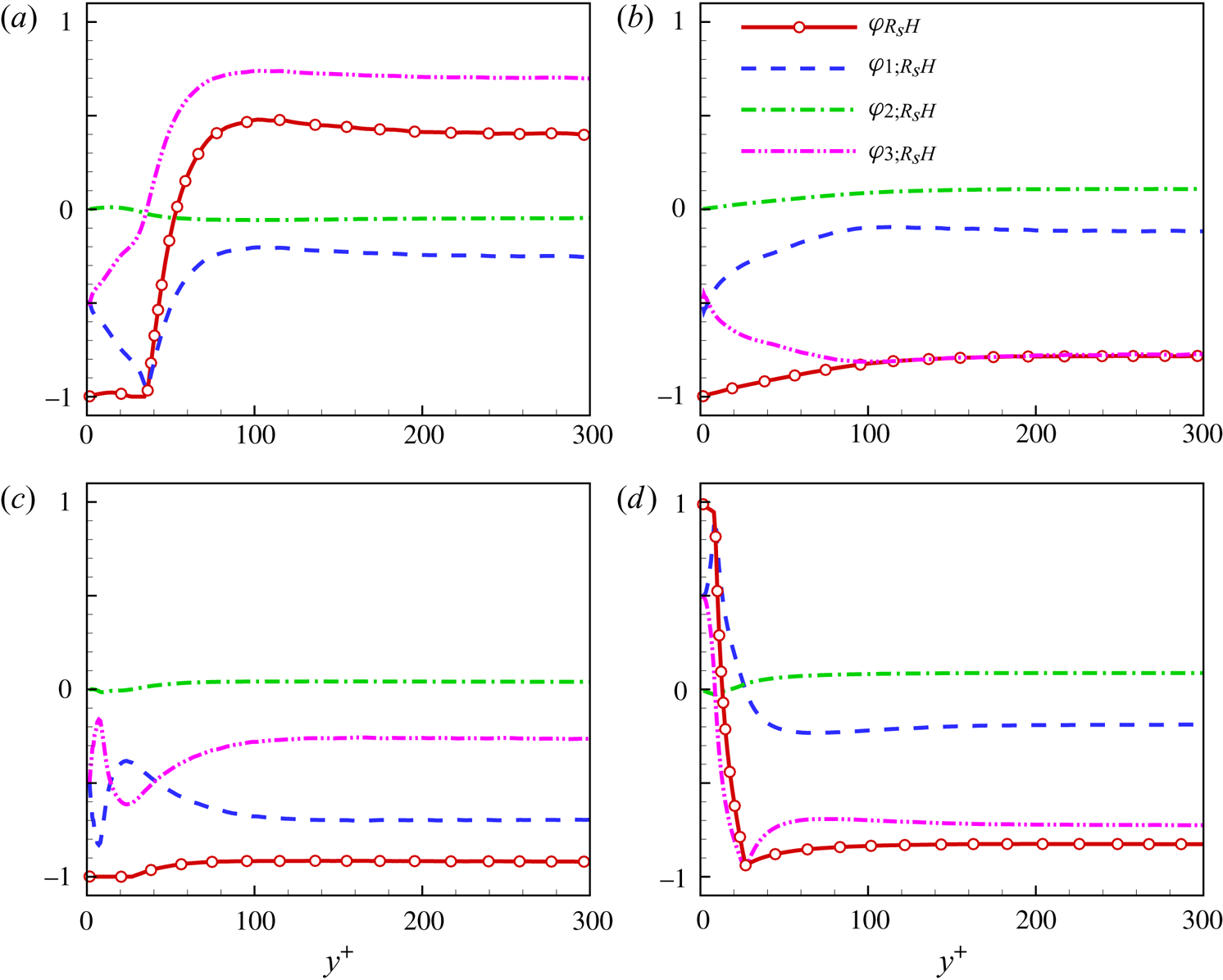
Figure 15(b) shows that for S1 topology, the promotion of the pressure-Hessian tensor on the first principal strain rate and its inhibition on the second principal strain rate cancel each other. Its contribution to dissipation is mainly reflected by its inhibition on the third principal strain rate in the channel's central region. In the vicinity of the channel wall, the pressure-Hessian tensor weakens the inhibition of the second and third principal strain rates. It enhances the promotion of the first principal strain rate, resulting in the weakening of the overall dissipation inhibition. Figure 15(c) shows that, for S3 topology, the pressure-Hessian tensor's effect on the first principal strain rate plays a dominant role, and its effect on the third principal strain rate is restrained, while its effect on the second principal strain rate is close to zero, which results in the promotion of overall dissipation in the channel's central region. Near the wall, the pressure-Hessian tensor's promotion effect on the first principal strain rate and the inhibition effect on the third principal strain rate are weakened. However, it promotes the generation of the second principal strain rate significantly, enhancing the dissipation in the viscous sublayer. Figure 15(d) shows that for the S2 topology, the effect of the pressure-Hessian tensor on the strain rate in the centre of the channel is consistent with that for the S1 topology. In the buffer layer and viscous sublayer, the pressure-Hessian tensor on the first principal strain rate changes from promotion to inhibition. Its effect on the third principal strain rate reaches the maximum relative inhibition at  $y^+ \approx 20$, and then gradually becomes promotion in the viscous sublayer.
Figure 16 shows the mechanisms of the effect of the pressure-Hessian tensor on the processes of dissipation generation  $R_S$ in different flow topological regions. Figure 16(a) shows that for the S4 topology, the promoting effect of the pressure-Hessian tensor on dissipation generation is mainly due to its action on the third principal strain rate, and its action on the first principal strain rate leads to the inhibition of dissipation generation, and the effect on the second principal strain rate has a relatively small mean contribution to dissipation generation. Near the wall, the pressure-Hessian tensor's suppression effect on the dissipation generation caused by the first principal strain rate's action increases relatively. However, the dissipation generation caused by its action on the third principal strain rate becomes suppressed, so the overall dissipation generation declines near the wall.
The profiles of  $\varphi _{R_SH}$,
 $\varphi _{1;R_SH}$,
 $\varphi _{2;R_SH}$ and
 $\varphi _{3;R_SH}$ versus
 $y^+$ for different flow topologies: (a) S4, (b) S1, (c) S3 and (d) S2.

As shown in figure 16(b,d), the influence of the pressure-Hessian tensor on dissipation generation in the outer layer of the channel for the S1 and S2 topologies is similar in the outer layer of the channel, which is controlled by the effect of the pressure-Hessian tensor on the third principal strain rate, inhibiting dissipation generation. Near the wall, in the S1 topological region, the inhibition effect of the pressure-Hessian tensor on the first principal strain rate enhances, while the inhibition effect on the third principal strain rate weakens. The effect of the pressure-Hessian tensor on the first and third principal strain rates leads to dissipation generation from inhibition to promotion in the S2 topological region. In the S3 topological region, the effect of the pressure-Hessian tensor on the first and third principal strain rates leads to the inhibition and dominance of dissipation generation, which leads to the inhibition of overall dissipation generation, as shown in figure 16(c).
Finally, the pressure-Hessian tensor's contribution to the enstrophy generation,  $R_\omega H$, is investigated. Figure 17 shows the wall-normal profiles of
 $\varphi _{R_\omega H}$ and its components versus
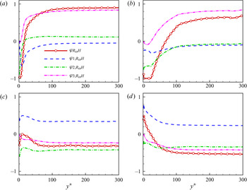
 $y^+$. As shown in figure 17(a,b), for the focused topologies S1 and S4, the pressure-Hessian tensor plays a significant role in promoting the enstrophy generation in the central region of the channel, mainly contributed by the third eigenvalue of the pressure-Hessian tensor. The reason is that in the topologies S1 and S4, the vorticity tends to be parallel to
 $\boldsymbol {f}_3$ in the third principal direction of the pressure-Hessian tensor and perpendicular to other principal directions (Lawson & Dawson Reference Lawson and Dawson2015). For S1 and S4 flow topologies, the vorticity tends to be aligned with the principal direction
 $\boldsymbol {f}_2$ near the wall. Therefore, the second eigenvalue's contribution gradually dominates, and the overall effect of the pressure-Hessian tensor tends to inhibit the enstrophy generation.
The profiles of  $\varphi _{R_\omega H}$,
 $\varphi _{1;R_\omega H}$,
 $\varphi _{2;R_\omega H}$ and
 $\varphi _{3;R_\omega H}$ versus
 $y^+$ for different flow topologies: (a) S4, (b) S1, (c) S3 and (d) S2.

As shown in figure 17(c,d), for the topologies S2 and S3, the effects of the first and second eigenvalues of the pressure-Hessian tensor on the generation term of enstrophy in the central region of the channel are opposite, and their amplitudes are approximately the same and cancel each other out. Finally,  $\varphi _{R_\omega H}$ has a similar distribution versus
 $y^+$ with
 $\varphi _{3;R_\omega H}$, which is shown to inhibit the enstrophy generation. Here, the vorticity tends to be distributed in the plane
 $\boldsymbol {f}_2$–
 $\boldsymbol {f}_3$. However, because the absolute value of
 $\eta _1$ is usually significant, its effect on the enstrophy generation term is still relatively strong. In the buffer layer, the vorticity tends to be distributed in the plane
 $\boldsymbol {f}_1$–
 $\boldsymbol {f}_2$, the effect of the third eigenvalue is small, and the effect of the first eigenvalue is relatively strong and dominant.
4.5. The effects of pressure-Hessian tensor on dynamic evolution of invariants
To further understand the effect of the pressure-Hessian tensor on invariants’ dynamic evolution, we will analyse its effect on the mean trajectories of invariants in the plane  $Q$–
 $R$. The conditional mean velocities of the invariants
 $Q$ and
 $R$ in the plane
 $Q$–
 $R$ can be split into
 $$\begin{gather} \boldsymbol{v}=\boldsymbol{v}_S+\boldsymbol{v}_H+\boldsymbol{v}_V, \end{gather}$$
 $$\begin{gather}\boldsymbol{v}_S=(v_{RS}, v_{QS})= \langle(RS,QS)\,| \,(R,Q)\rangle, \end{gather}$$
 $$\begin{gather}\boldsymbol{v}_H=(v_{RH}, v_{QH})= \langle(RH,QH)\,| \,(R,Q)\rangle, \end{gather}$$
 $$\begin{gather}\boldsymbol{v}_V=(v_{RV}, v_{QV})= \langle(RV,QV)\,| \,(R,Q)\rangle, \end{gather}$$
in which  $\boldsymbol {v}_S$,
 $\boldsymbol {v}_H$ and
 $\boldsymbol {v}_V$ represent the contributions of nonlinear interaction, the pressure-Hessian tensor and viscosity to the conditional mean velocity, respectively.
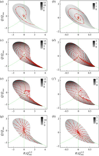
Figure 18 shows the streamlines (i.e. CMTs) corresponding to conditional mean velocity vectors of invariants  $Q$ and
 $R$. As shown in figure 18(a,b), the CMT of invariants given by
 $\boldsymbol {v}$ converges to the origin clockwise in the channel's central region and it diverges clockwise outwards in the buffer layer, similar to previous studies for wall turbulence (Elsinga & Marusic Reference Elsinga and Marusic2010; Atkinson et al. Reference Atkinson, Chumakov, Bermejo-Moreno and Soria2012; Chu & Lu Reference Chu and Lu2013; Bechlars & Sandberg Reference Bechlars and Sandberg2017). Figure 18(c,d) shows that the velocity
 $\boldsymbol {v}_S$ due to the nonlinear interaction of the invariants prompts the invariants to evolve from
 $(R,Q) = (-\infty, -\infty )$ to
 $(R,Q) = (+\infty, -\infty )$ along the curve
 $\varDelta =0$, similar to the property that the invariants tend to diverge in the RE equations. The viscosity term reflects the dissipation of the invariant, which makes the streamline converge to the origin, as shown in figure 18(g,h). It should be emphasized that the contribution of the pressure-Hessian term is opposite to that of the nonlinear interaction term, which makes the invariants evolve from
 $(R, Q)=(+\infty, -\infty )$ to
 $(R, Q)=(-\infty,-\infty )$ along the right branch of the curve
 $\varDelta = 0$ (see figure 18e, f). It is this behaviour of the pressure Hessian that resists the divergent effect of the RE equation on the invariants (Lüthi et al. Reference Lüthi, Holzner and Tsinober2009; Meneveau Reference Meneveau2011; Wilczek & Meneveau Reference Wilczek and Meneveau2014; Lawson & Dawson Reference Lawson and Dawson2015).
The streamlines (i.e. CMTs) corresponding to conditional mean velocity vectors of invariants  $Q$ and
 $R$: (a,b)
 $\boldsymbol {v}$; (c,d)
 $\boldsymbol {v}_S$; (e, f)
 $\boldsymbol {v}_H$; and (g,h)
 $\boldsymbol {v}_V$. Panels (a,c,e,g) show the statistical results in the central plane of the channel (
 $y^+=532$). Panels (b,d,f ,h) show the statistical results in the buffer layer (
 $y^+=20.5$). The background colours denote the amplitude of the corresponding vector, and the region of joint p.d.f. value less than
 $10^{-4} \max [\mathrm {p.d.f.} (R,Q) ]$ is omitted. Here, the physical quantities are normalized by the root mean square of fluctuating
 $Q$.

Figure 18(e) further shows that in the central region of the channel, there is a region of the S1 topology caused by the pressure-Hessian effect that drives the invariant to spin outwards anticlockwise, where the term  $\boldsymbol {v}_H$ is very weak. This feature changes significantly in the buffer layer, as shown in figure 18( f). The anticlockwise spiral region caused by the pressure-Hessian tensor becomes divergent from the asymptote to the left-hand and right-hand sides, and the streamline is nearly parallel to the
 $R$-axis. The above results lead, in the nearby region of
 $R>0, Q=0$, to the pressure-Hessian tensor making the invariant
 $R$ tend to diverge, but its effect on
 $Q$ is relatively tiny.
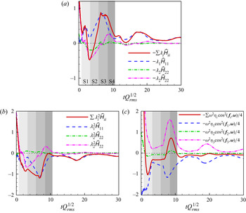
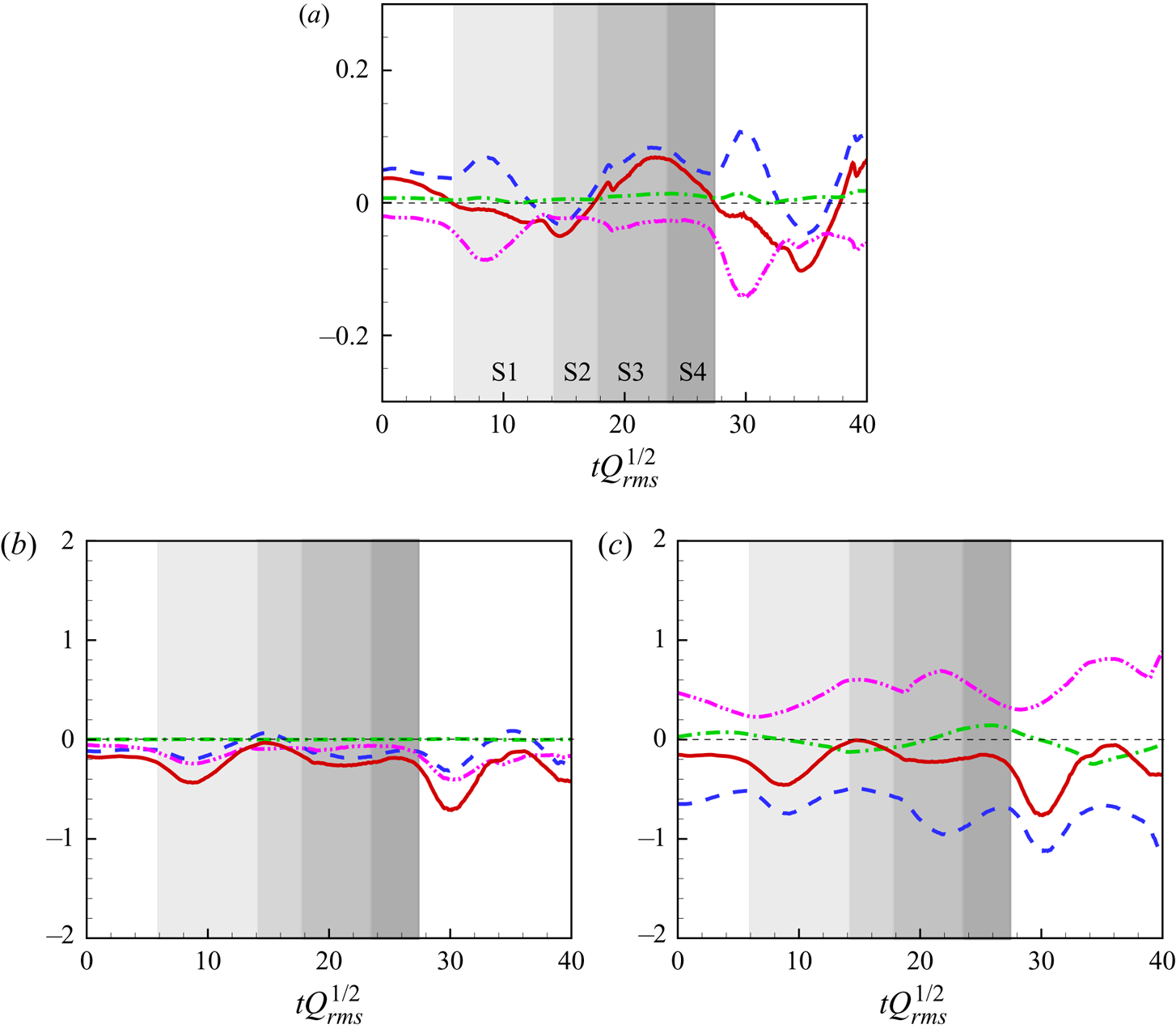
To further understand the effects of the pressure-Hessian tensor on the CMTs of invariants, figure 19 shows the evolution of the pressure-Hessian's contribution along the mean trajectory of invariants (see figure 18a) in the channel's centre, in which the contribution has been decomposed by (3.13)–(3.15). Figure 19(a,b) shows that the effect of the pressure-Hessian tensor on the dynamic evolution of  $Q_S$ and
 $R_S$ is mainly realized by acting on the first principal strain rate. The more the invariant evolves to the origin, the more dominant is the effect on the first principal strain rate. The pressure-Hessian tensor enhances the dissipation of mechanical energy (i.e.
 $-Q_S$) by promoting the first principal strain rate but inhibits the nonlinear generation rate of dissipation (i.e.
 $R_S$). As shown in figure 19(c), the first eigenvalue of the pressure-Hessian tensor suppresses
 $R_\omega$, the third eigenvalue promotes
 $R_\omega$, and the competition between them determines the effect of the pressure-Hessian tensor on the evolution of
 $R_\omega$, while the contribution of the second eigenvalue is relatively small. According to the definition of the eigenvalues, the pressure-Hessian tensor's first eigenvalue generally has a more significant absolute value. Thus, the corresponding term's contribution along the CMT is more productive than that of the third eigenvalue most of the time.
In the central plane of the channel ( $y^+=532$), the pressure-Hessian's contribution to the invariant dynamics along the CMT of invariants in figure 18(a): (a)
 $Q_S H$, (b)
 $R_S H$ and (c)
 $R_\omega H$. The shadow colour from light to dark indicates the time period of the CMT in the four flow topologies of S1–S4.

Figure 20 shows the evolution of the contribution of the pressure-Hessian tensor along the mean trajectory of invariants in figure 18(b). As shown in figure 20(a), in the buffer layer, the pressure-Hessian tensor inhibits the first principal strain rate in the evolution process of invariants from topology S1 to topology S2 and promotes it in other topological regions, while it always restrains the third principal strain rate. Because of the competition between them, when the invariants are in the regions of flow topologies S1 and S2, the pressure-Hessian tensor suppresses the dissipation. It makes the invariant  $Q$ tend to increase. When the invariants are in the regions of flow topologies S3 and S4, the pressure-Hessian tensor promotes the dissipation and makes the invariant
 $Q$ tend to decrease. The above results are consistent with the clockwise evolution of invariants. Figure 20(b) shows that the contribution of the pressure-Hessian tensor to the dynamics of
 $R_S$ is always negative, which is shown as the inhibition of dissipation generation. Figure 20(c) shows that the pressure-Hessian tensor also inhibits the generation of enstrophy, which is similar to the statistical results in the central region of the channel.
In the buffer layer ( $y^+= 20.5$), the pressure-Hessian's contribution to the invariant dynamics evolves along the CMT of invariants in figure 18(b): (a)
 $Q_S H$, (b)
 $R_S H$ and (c)
 $R_\omega H$. The shadow colour from light to dark indicates the time period of the CMT in the four flow topologies of S1–S4. The legends of the various lines are the same as those in figure 19.

It is noted that the mean contribution of the pressure-Hessian tensor to invariant dynamics in the different flow topologies shown in figures 15–17 is inconsistent with the contribution of the pressure-Hessian tensor to invariant dynamics along the mean trajectory of invariants shown in figures 19–20. This is because the former is the mean behaviour of all the invariants in the same flow topology and the p.d.f. of the invariants is centralized at the origin, resulting in the fact that it better reflects the contribution of the pressure-Hessian tensor when the magnitude of the invariants is small.
The results above reveal the significant effects of inhomogeneity and anisotropy on pressure-Hessian statistics, based on the analysis of the instantaneous pressure-Hessian tensor at different wall-normal positions. However, it is unclear whether the inhomogeneity and anisotropy originate directly from the mean shear flow or the inhomogeneous and anisotropic fluctuating flow. The method of pressure decomposition (Tang et al. Reference Tang, Zhao, Wan and Liu2020) provides a chance to achieve more physical understanding. In our previous study (Tang et al. Reference Tang, Zhao, Wan and Liu2020), with the purpose of investigating the statistical characteristics of pressure fluctuations in compressible channel turbulence, we decomposed the pressure fluctuations into the fast pressure  $p_r$, slow pressure
 $p_s$, Stokes pressure
 $p_ \tau$ and compressible pressure
 $p_c$. The fast pressure represents the pressure fluctuations generated by the interaction between turbulent fluctuations and the mean flow. The slow pressure represents the fluctuations induced by the interactions between turbulent fluctuations. The wall boundary condition causes the Stokes pressure, and the compressible pressure is defined as the difference between the total pressure and the other pressure components (Sarkar Reference Sarkar1992).
To evaluate which pressure mechanism contributes the most to the pressure-Hessian terms, we also decompose the pressure-Hessian tensor. Firstly, the instantaneous pressure is split in terms of the mean pressure and the fluctuation. Then the fluctuating pressure is decomposed following the method in Tang et al. (Reference Tang, Zhao, Wan and Liu2020). In turn, the derivatives of each pressure part are computed to obtain the corresponding pressure-Hessian part. The decomposition of the pressure-Hessian tensor reads
 \begin{equation} \boldsymbol{\mathsf{H}} = \boldsymbol{\mathsf{H}}_{r} + \boldsymbol{\mathsf{H}}_{s} + \boldsymbol{\mathsf{H}}_{\tau} + \boldsymbol{\mathsf{H}}_{c} + { \boldsymbol{\mathsf{H}}}_m, \end{equation}
where the subscripts  $r$,
 $s$,
 $\tau$,
 $c$ and
 $m$ represent the pressure-Hessian corresponding to the rapid, slow, Stokes, compressible and mean pressure. Since the pressure-Hessian tensor in (A3), (A5) and (A7)–(A9) is linear, their contributions to the evolution of invariants can also be decomposed into the corresponding part of (4.7), and the conditional mean vector
 $\boldsymbol {v}_H$ in the
 $Q$–
 $R$ plane becomes
 \begin{equation} \boldsymbol{v}_H=\boldsymbol{v}_{H_r} +\boldsymbol{v}_{H_s} +\boldsymbol{v}_{H_\tau}+\boldsymbol{v}_{H_c}+{\boldsymbol{v}}_{H_m}. \end{equation}
In the central region of the channel, the slow-pressure-related term is expected to play a dominant role due to the nearly zero mean shear (Gerolymos, Sénéchal & Vallet Reference Gerolymos, Sénéchal and Vallet2013). To investigate the relative importance of each component of the conditional mean vector  $\boldsymbol {v}_H$ in the near-wall region, figure 21 shows the relative proportion of the amplitude of each term in (4.8) in the buffer layer, respectively. It is found that the relative amplitude of the conditional mean velocity for the slow-pressure-related term in the buffer layer is dominant in most areas of the
 $Q$–
 $R$ plane, and the proportion of the amplitude is above
 $70\,\%$. In the S1 topological region, there is a region where the proportion of the amplitude of
 $\boldsymbol {v}_{H_s}$ is between
 $50\,\%$ and
 $60\,\%$. The proportion of the amplitude of
 $\boldsymbol { v }_{H_r}$ can reach more than
 $30\,\%$, which also plays a certain role in the contribution of the overall pressure-Hessian tensor. The contribution of other pressure terms (e.g. wall boundary, compressibility and mean pressure gradient) is tiny, almost no more than
 $10\,\%$. Further comparison shows that the region with smaller proportion of the amplitude of
 $\boldsymbol {v}_{H_s}$ is consistent with the region with small amplitude of
 $\boldsymbol {v}_{H}$ in figure 18( f), which further illustrates the dominance of the slow-pressure-related term.
The conditional mean vector  $\boldsymbol {v}_H$ of the pressure-Hessian's contribution to the invariant dynamics in the buffer layer (
 $y^+=20.5$), which is decomposed by (4.8). The proportion of the amplitude of each part is: (a)
 $|\boldsymbol {v}_{H_s}|/ \sum |\boldsymbol {v}_i |$, (b)
 $| \boldsymbol {v}_{H_r} | / \sum | \boldsymbol {v}_i |$ and (c)
 $(|\boldsymbol {v}_{H_\tau }|+|\boldsymbol {v}_{H_c}| +|\boldsymbol {v}_{H_m}|)/ \sum | \boldsymbol {v}_i |$, where
 $i=H_r, H_s, H_c, H_\tau, H_m$.

Since the VGT represents the small-scale properties of flow (Meneveau Reference Meneveau2011), the pressure-Hessian term in the evolution equation of invariants directly affected by the large-scale mean shear is limited. Nevertheless, by analysing the geometrical relationships between the pressure-Hessian tensor and the vorticity/strain-rate tensor, and its contribution to invariant dynamics, it is shown that the statistical properties of the pressure-Hessian tensor and its effect on the evolution of invariants are still affected by inhomogeneity and anisotropy. Combined with the analysis of pressure decomposition, this proves that the influence of inhomogeneity and anisotropy on the pressure-Hessian is mainly due to the inhomogeneity and anisotropy of velocity fluctuations near the wall. As far as the VGT modelling is concerned, the present results indicate that keeping only the pressure-Hessian contributions associated with the slow pressure may be adequate to capture the main characters of inhomogeneity and anisotropy, i.e. the pressure-Hessian tensor in (3.13)–(3.15) can be further approximated by the component corresponding to the slow pressure.
4.6. Modelling implications for VGT dynamics
The main findings of the present work focus on the characteristics of the pressure-Hessian contributions to the dynamical evolution of VGT invariants in wall turbulence. Instructive implications can be obtained as far as the modelling of VGT dynamics is concerned.
The conventional works for models of VGT dynamics are usually done in the fixed Cartesian coordinate system (Girimaji & Pope Reference Girimaji and Pope1990; Chevillard & Meneveau Reference Chevillard and Meneveau2006; Suman & Girimaji Reference Suman and Girimaji2009; Meneveau Reference Meneveau2011; Wilczek & Meneveau Reference Wilczek and Meneveau2014; Johnson & Meneveau Reference Johnson and Meneveau2016; Pereira, Moriconi & Chevillard Reference Pereira, Moriconi and Chevillard2018), where all the terms are tensorial (see (3.9)). Although significant improvements in the understanding and modelling of VGT dynamics have been obtained in the past decades, modelling work in wall turbulence is rare. Based on the present results, we think that developing a VGT model in the principal coordinate system of the strain-rate tensor may be more tractable than that in the conventional fixed coordinate system. The starting point should be the dynamics equations of the VGT in the principal coordinates (Lawson & Dawson Reference Lawson and Dawson2015) as shown by (A11)–(A13). The unclosed terms for an autonomous system of a dynamical model of the VGT are the pressure-Hessian tensor and viscous terms. The modelling of the former is still the main story, while the latter may be modelled adequately by the damping effects (Meneveau Reference Meneveau2011).
It may be feasible to build a model of the VGT that can faithfully capture the dynamics of invariants by properly simplifying (A11)–(A13). Based on the statistics of the geometric relationship between the pressure-Hessian tensor and the strain-rate tensor, it is reasonable to prescribe the eigenvectors of the pressure Hessian,  $\boldsymbol {f}_i$, to be random distributions centred at the configuration with the highest probability (see figure 12). A Gaussian random distribution might be a good choice, by which the pressure-Hessian tensor can be represented as an approximation comprising the eigenvalues of the pressure-Hessian tensor,
 $\eta _i$, and the eigenvectors of the strain-rate tensor,
 $\boldsymbol {e}_i$. Similarly, the product of pressure Hessian and vorticity in (A13) can also be represented approximately by
 $\eta _i$,
 $\boldsymbol {e}_i$ and the amplitude of vorticity, based on the geometric relationship between the pressure-Hessian tensor and the vorticity vector. As for the eigenvalues of the pressure-Hessian tensor, it is seen that
 $\eta _i$ are not sensitive to the mean shear (see figure 10). This implies that a model of
 $\eta _i$ from isotropic turbulence may be adequate to reproduce the main features of VGT dynamics. To the best of our knowledge, the theoretical frame based on Gaussian random velocity fields proposed by Wilczek & Meneveau (Reference Wilczek and Meneveau2014) is promising to perform the modelling of
 $\eta _i$.
It should be mentioned that a transition model connecting the near-wall (inhomogeneous and anisotropic) statistics and the nearly homogeneous and isotropic statistics in the central channel is still needed for a practical model of VGT dynamics. The fluid particles may transfer from the near-wall region to the central region of the channel and vice versa. The present results illustrate that the statistics of the pressure-Hessian tensor in the near-wall region may be significantly different from those in the central channel domain, i.e. the degree of inhomogeneity and anisotropy varies along the wall-normal direction. Thus, a transition model mimicking the quantitative dependence of inhomogeneity and anisotropy of the pressure-Hessian tensor on  $y^+$ is desired. However, the development of such a transition model is definitely a tough task, which requires a lot of efforts in the future.
5. Summary and conclusion
This study investigates the DNS data of a weakly compressible turbulent channel flow with a bulk Mach number of 1.56. The geometrical relationships between the pressure-Hessian tensor and the vorticity/strain-rate tensor, and the effect of the pressure-Hessian tensor on the dynamic evolution of velocity gradient invariants are studied. The main findings of this study are addressed as follows.
Firstly, in the centre of the channel, the vorticity tends to be aligned with the pressure-Hessian tensor's principal direction  $\boldsymbol {f}_3$ in the rotation-dominant region, which is consistent with the finding of isotropic turbulence. In the topological regions of S2 and S3, the vorticity tends to distribute in the plane
 $\boldsymbol {f}_2$–
 $\boldsymbol {f}_3$. However, in the buffer layer, the vorticity tends to be parallel to
 $\boldsymbol {f}_1$ or
 $\boldsymbol {f}_2$ in the S1 topological region. In the S4 topological region, the vorticity gradually evolves from being parallel to
 $\boldsymbol {f}_3$ to being parallel to
 $\boldsymbol {f}_1$ with the decrease of wall distance. In the topological regions of S2 and S3, the vorticity tends to lie in the plane
 $\boldsymbol {f}_1$–
 $\boldsymbol {f}_2$.
Secondly, the geometrical relationships between the principal directions of the pressure-Hessian tensor and the principal axes of the strain-rate tensor are consistent with the isotropic turbulence in the central region of the channel. Whereas, in the buffer layer, the principal direction of the pressure-Hessian tensor  $\boldsymbol {f}_2$ tends to be aligned with
 $\boldsymbol {e}_2$, and
 $\boldsymbol {f}_1$ and
 $\boldsymbol {f}_3$ tend to be distributed in the plane
 $\boldsymbol {e}_1$–
 $\boldsymbol {e}_3$, and the angle with
 $\boldsymbol {e}_1$ is
 ${\rm \pi} /4$.
Thirdly, in the central region, the effect of the pressure-Hessian tensor on the third principal strain rate dominates the promotion of the topology S4 on dissipation generation and the suppression of the topologies S1 and S2 on dissipation and its generation. The effect of the pressure-Hessian tensor on the first principal strain rate dominates the promotion of the topology S3 on dissipation. The effects of the pressure-Hessian tensor on the first and third principal strain rates jointly dominate the promotion effects of the topology S1 on dissipation and the suppression of the topology S3 on dissipation generation. While, in the buffer layer, the effects of the pressure-Hessian tensor on the first and third principal strain rates jointly dominate dissipation and generation. The mean contribution of the pressure-Hessian tensor to the dynamics of enstrophy generation is directly affected by the distribution of the angles between the eigenvectors of the pressure-Hessian tensor and the vorticity, where the third- or first-eigenvalue-related terms play the dominant roles.
Finally, the evolution of the contribution of the pressure-Hessian tensor to the dynamics of invariants along the CMT shows that the contribution of the pressure-Hessian tensor to dissipation dynamics is jointly determined by the effects of the pressure-Hessian tensor on the first and third principal strain rates. The contribution of the pressure-Hessian tensor to the nonlinear generation of dissipation is mainly dominated by its impact on the first principal strain rate. The contribution of the pressure-Hessian tensor to the enstrophy generation depends on the competition between the first and third eigenvalues of the pressure-Hessian tensor. Furthermore, the decomposition of the pressure-Hessian tensor shows that the slow-pressure-related term plays a dominant role in the contribution of the pressure-Hessian tensor to the dynamics of VGT invariants. The anisotropy and inhomogeneity of the pressure-Hessian tensor's contribution terms mainly come from the anisotropy and inhomogeneity of velocity fluctuation.
In short, the above findings for the fundamental properties of the pressure Hessian tensor in this weakly compressible turbulent channel flow would be instructive in formulating dynamical equations of the VGT for inhomogeneous turbulence, and imply that developing a VGT model in the principal coordinate system of the strain-rate tensor may be feasible. It is promising to make some simplifications of the pressure-Hessian tensor's contribution to the VGT dynamics based on the present statistics. Nevertheless, there are still many challenges in the access to develop a practical model of VGT dynamics in wall turbulence.
Acknowledgements
The numerical calculations in this paper have been done on the supercomputing system in the Supercomputing Center of University of Science and Technology of China (USTC).
Funding
This work is supported by the National Natural Science Foundation of China under grants 12172351, 92052301, 91952103, 92152301 and 11621202, by the Fundamental Research Funds for the Central Universities, by the National Numerical Windtunnel Project, and by the USTC Research Funds of the Double First-Class Initiative.
Declaration of interests
The authors report no conflict of interest.
Appendix A. The VGT invariants and evolution equations
Based on the definitions, the VGT invariants can be evaluated from the components of the strain-rate tensor ( $\boldsymbol{\mathsf{S}}$) and the rotation-rate tensor (
 $\boldsymbol{\mathsf{W}}$) as
 $$\begin{gather} P ={-}\mathrm{tr}( \boldsymbol{\mathsf{A}})=-{\mathsf{S}}_{kk}, \end{gather}$$
 $$\begin{gather}Q = \tfrac{1}{2}[\mathrm{tr}(\boldsymbol{\mathsf{A}})^2 -\mathrm{tr}(\boldsymbol{\mathsf{A}}^2)] = \tfrac{1}{2}(P^2-{\mathsf{S}}_{ij}{\mathsf{S}}_{ij}+{\mathsf{W}}_{ij}{\mathsf{W}}_{ij}), \end{gather}$$
 $$\begin{gather}R ={-}\mathrm{det}( \boldsymbol{\mathsf{A}}) ={-}\tfrac{1}{3}P^3+PQ-\tfrac{1}{3}{\mathsf{S}}_{ij}{\mathsf{S}}_{jk}{\mathsf{S}}_{ki} -{\mathsf{W}}_{ij}{\mathsf{W}}_{jk}{\mathsf{S}}_{ik}, \end{gather}$$
where  $\text {tr}(\cdot )$ and
 $\text {det}(\cdot )$ denote the trace and determinant of a tensor, respectively. Similarly, the invariants of
 $\boldsymbol{\mathsf{S}}$ and
 $\boldsymbol{\mathsf{W}}$ are obtained as
 $$\begin{gather} P_S = P = -{\mathsf{S}}_{kk}, \quad Q_S = \tfrac{1}{2}(P_S^2-{\mathsf{S}}_{ij}{\mathsf{S}}_{ij}), \quad R_S ={-}\tfrac{1}{3}P^3+P_SQ_S -\tfrac{1}{3}{\mathsf{S}}_{ij}{\mathsf{S}}_{jk}{\mathsf{S}}_{ki}, \end{gather}$$
 $$\begin{gather}P_W=0, \quad Q_W =\tfrac{1}{2}{\mathsf{W}}_{ij}{\mathsf{W}}_{ij}, \quad R_W=0. \end{gather}$$
The evolution equations of the second invariants ( $Q,Q_S,Q_W$) can be obtained from the definitions of the invariants and (3.9) as (Chu & Lu Reference Chu and Lu2013; Bechlars & Sandberg Reference Bechlars and Sandberg2017)
 \begin{gather}
\frac{\mathcal{D}Q_S}{\mathcal{D}t} = \frac{\partial
Q_S}{\partial t} + \underbrace{\boldsymbol{u}\boldsymbol{\cdot}\boldsymbol{\nabla}Q_S}_{Q_S
C} = \underbrace{(P(P^2-2Q)+\boldsymbol{\mathsf{S}}\boldsymbol{:}
(\boldsymbol{\mathsf{S}}^2+\boldsymbol{\mathsf{W}}^2)+\tfrac{2}{3}P\,\mathrm{tr}
(\boldsymbol{\mathsf{H}}))}_{Q_S S} \nonumber\\
\hspace{13.5pc}+ \underbrace{\boldsymbol{\mathsf{S}}\boldsymbol{:}
\tilde{\boldsymbol{\mathsf{H}}}}_{Q_S H}
+\underbrace{(P\,\mathrm{tr}(\boldsymbol{\mathsf{B}})
+\boldsymbol{\mathsf{S}}\boldsymbol{:}\boldsymbol{\mathsf{B}})}_{Q_S B}
\underbrace{-(P\,\mathrm{tr}(\boldsymbol{\mathsf{V}})
+\boldsymbol{\mathsf{S}}\boldsymbol{:}\boldsymbol{\mathsf{V}})}_{Q_S
V} ,
\end{gather}
 \begin{gather}
\frac{\mathcal{D}Q_W}{\mathcal{D}t}= \frac{\partial Q_W}{\partial t} +
\underbrace{\boldsymbol{u}\boldsymbol{\cdot}\boldsymbol{\nabla}Q_W}_{Q_W C} =
\underbrace{2\boldsymbol{\mathsf{S}}\boldsymbol{:}\boldsymbol{\mathsf{W}}^2}_{Q_W
S}
\underbrace{-\boldsymbol{\mathsf{W}}\boldsymbol{:}\boldsymbol{\mathsf{B}}}_{Q_W
B} +
\underbrace{\boldsymbol{\mathsf{W}}\boldsymbol{:}\boldsymbol{\mathsf{V}}}_{Q_W V},
\end{gather}
and
 \begin{align} \frac{\mathcal{D}Q}{\mathcal{D}t} = \frac{\partial Q}{\partial t} + \underbrace{\boldsymbol{u}\boldsymbol{\cdot}\boldsymbol{\nabla}Q}_{Q C} &= \underbrace{(PQ-3R+\tfrac{2}{3}P\,\mathrm{tr}(\boldsymbol{\mathsf{H}}))}_{QS} + \underbrace{(P\,\mathrm{tr}(\boldsymbol{\mathsf{B}})+(\boldsymbol{\mathsf{S}} -\boldsymbol{\mathsf{W}})\boldsymbol{:}\boldsymbol{\mathsf{B}})}_{QB} \nonumber\\ &\quad + \underbrace{\boldsymbol{\mathsf{S}}\boldsymbol{:} \tilde{\boldsymbol{\mathsf{H}}}}_{QH} \underbrace{-(P\,\mathrm{tr}(\boldsymbol{\mathsf{V}}) +(\boldsymbol{\mathsf{S}}-\boldsymbol{\mathsf{W}})\boldsymbol{:}\boldsymbol{\mathsf{V}})}_{QV}, \end{align}
where  $(\boldsymbol \ast )\boldsymbol {:}(\boldsymbol \ast )=(\ast )_{ij}(\ast )_{ij}$ is the quadratic contraction of two tensors, and the square of a tensor is denoted as
 $[(\ast )^2]_{ij}= (\ast )_{ik}(\ast )_{kj}$. The physical meanings of each item in (A3)–(A5) are as follows (Pirozzoli & Grasso Reference Pirozzoli and Grasso2004; Chu & Lu Reference Chu and Lu2013):
 $Q_SS$ is the nonlinear generation term of
 $Q_S$, including the effects of self-amplification of strain, i.e.
 $\boldsymbol{\mathsf{S}}\boldsymbol {:}\boldsymbol{\mathsf{S}}^2$, the strain–vorticity interaction, i.e.
 $\boldsymbol{\mathsf{S}}\boldsymbol {:}\boldsymbol{\mathsf{W}}^2$, and the action of dilatation;
 \begin{equation} Q_WS = 2 \boldsymbol{\mathsf{S}}\boldsymbol{:}\boldsymbol{\mathsf{W}}^2 = \tfrac{1}{2}\boldsymbol{\omega}\boldsymbol{\cdot} \boldsymbol{\mathsf{S}}\boldsymbol{\cdot}\boldsymbol{\omega} + 2PQ_W \end{equation}
is a generation term of enstrophy;  $QS$ is a generation term of
 $Q$ due to interactions of invariants;
 $Q_SH$ and
 $QH$ represent the contribution of the anisotropic part of the pressure-Hessian tensor;
 $Q_SB$,
 $Q_WB$ and
 $QB$ are related to the baroclinic effect; and
 $Q_SV$,
 $Q_WV$ and
 $QV$ denote the viscous effect. It is noted that the pressure-Hessian tensor has no direct contribution to the generation of enstrophy. Only when the density gradient does not coincide with the pressure gradient does the baroclinic effect occur, and then the pressure will directly affect the generation of enstrophy.
Similarly, the evolution equations for  $R_s$ and
 $R_\omega$ can be obtained as follows:
 \begin{align} \frac{\mathcal{D} R_S}{\mathcal{D}t} &= \frac{\partial R_S}{\partial t}+ \underbrace{\boldsymbol{u}\boldsymbol{\cdot}\boldsymbol{\nabla} R_S}_{R_S C} \nonumber\\ &= \underbrace{(PR_S-2Q_SQ_W+(P\boldsymbol{\mathsf{S}} +\boldsymbol{\mathsf{S}}^2)\boldsymbol{:}\boldsymbol{\mathsf{W}}^2 +\tfrac{1}{3}Q_S\,\mathrm{tr}(\boldsymbol{\mathsf{H}}) )}_{R_SS} + \underbrace{( P\boldsymbol{\mathsf{S}}\boldsymbol{:}\tilde{\boldsymbol{\mathsf{H}}} +\boldsymbol{\mathsf{S}}^2\boldsymbol{:}\tilde{\boldsymbol{\mathsf{H}}} )}_{R_SH} \nonumber\\ &\quad + \underbrace{(P\boldsymbol{\mathsf{S}}\boldsymbol{:}\boldsymbol{\mathsf{B}} +Q_S\,\mathrm{tr}(\boldsymbol{\mathsf{B}}) +\boldsymbol{\mathsf{S}}^2\boldsymbol{:}\boldsymbol{\mathsf{B}} )}_{R_SB} - \underbrace{(P\boldsymbol{\mathsf{S}}\boldsymbol{:}\boldsymbol{\mathsf{V}} +Q_S\,\mathrm{tr}(\boldsymbol{\mathsf{V}}) +\boldsymbol{\mathsf{S}}^2\boldsymbol{:}\boldsymbol{\mathsf{V}} )}_{R_SV} \end{align}
and
 \begin{align} \frac{\mathcal{D}
R_\omega}{\mathcal{D}t} &= \frac{\partial
R_\omega}{\partial t}+
\underbrace{\boldsymbol{u}\boldsymbol{\cdot}\boldsymbol{\nabla}
R_\omega}_{R_\omega C} \nonumber\\ &= \underbrace{ (
(2P\boldsymbol{\mathsf{S}}+\boldsymbol{\mathsf{S}}^2)\boldsymbol{:}\boldsymbol{\mathsf{W}}^2
-P^2Q_W-2Q_SQ_W-\tfrac{1}{3}Q_W\,\mathrm{tr}(\boldsymbol{\mathsf{H}}))}_{R_\omega
S}
\underbrace{-\tfrac{1}{4}\boldsymbol{\omega}\boldsymbol{\cdot}
\tilde{\boldsymbol{\mathsf{H}}}\boldsymbol{\cdot}\boldsymbol{\omega}}_{R_\omega
H} \nonumber\\ &\quad +
\underbrace{(P\boldsymbol{\mathsf{W}}\boldsymbol{:}\boldsymbol{\mathsf{B}}
-Q_W\,\mathrm{tr}(\boldsymbol{\mathsf{B}})
+(\boldsymbol{\mathsf{S}}\boldsymbol{\cdot}\boldsymbol{\mathsf{W}}
+\boldsymbol{\mathsf{W}}\boldsymbol{\cdot}\boldsymbol{\mathsf{S}}
-\boldsymbol{\mathsf{W}}\boldsymbol{\cdot}\boldsymbol{\mathsf{W}})\boldsymbol{:}
\boldsymbol{\mathsf{B}})}_{R_\omega B} \nonumber\\
& \quad \underbrace{-(P\boldsymbol{\mathsf{W}}\boldsymbol{:}\boldsymbol{\mathsf{V}}
-Q_W\,\mathrm{tr}(\boldsymbol{\mathsf{V}})
+(\boldsymbol{\mathsf{S}}\boldsymbol{\cdot}\boldsymbol{\mathsf{W}}
+\boldsymbol{\mathsf{W}}\boldsymbol{\cdot}\boldsymbol{\mathsf{S}}
-\boldsymbol{\mathsf{W}}\boldsymbol{\cdot}\boldsymbol{\mathsf{W}})\boldsymbol{:}
\boldsymbol{\mathsf{V}})}_{R_\omega V} .
\end{align}
So the evolution equation of  $R$ is (Chu & Lu Reference Chu and Lu2013)
 \begin{align} \frac{\mathcal{D} R}{\mathcal{D}t} &=\frac{\mathcal{D} (R_S-R_\omega)}{\mathcal{D}t}= \frac{\partial R}{\partial t}+ \underbrace{\boldsymbol{u}\boldsymbol{\cdot}\boldsymbol{\nabla} R}_{RC} \nonumber\\ &= \underbrace{( P\boldsymbol{\mathsf{S}}\boldsymbol{:}\tilde{\boldsymbol{\mathsf{H}}} +(\boldsymbol{\mathsf{S}}^2+\boldsymbol{\mathsf{W}}^2)\boldsymbol{:} \tilde{\boldsymbol{\mathsf{H}}})}_{RH} + \underbrace{(P(\boldsymbol{\mathsf{S}}-\boldsymbol{\mathsf{W}}) \boldsymbol{:}\boldsymbol{\mathsf{B}}+Q\,\mathrm{tr}(\boldsymbol{\mathsf{B}}) +(\boldsymbol{\mathsf{S}}-\boldsymbol{\mathsf{W}})^2\boldsymbol{:}\boldsymbol{\mathsf{B}})}_{RB} \nonumber\\ &\quad + \underbrace{(PR+\tfrac{1}{3}Q\,\mathrm{tr}(\boldsymbol{\mathsf{H}}))}_{RS} \underbrace{-(P(\boldsymbol{\mathsf{S}}-\boldsymbol{\mathsf{W}})\boldsymbol{:} \boldsymbol{\mathsf{V}}+Q\,\mathrm{tr}(\boldsymbol{\mathsf{V}}) +(\boldsymbol{\mathsf{S}}-\boldsymbol{\mathsf{W}})^2\boldsymbol{:}\boldsymbol{\mathsf{V}} )}_{RV} . \end{align}
The above equations (A3)–(A5) and (A7)–(A9) describe the evolution of  $R$ involving dissipation, enstrophy and their mutual competition, and the dynamic equations of the three generation mechanisms, which mainly include the nonlinear generation term and pressure-Hessian term, baroclinic term and viscous term, of which the pressure-Hessian term is the focus of this study.
By denoting the eigenvectors of the strain-rate tensor ( $\boldsymbol{\mathsf{S}}$) as
 $\boldsymbol {e}_1,\ \boldsymbol {e}_2,\ \boldsymbol {e}_3$, and the corresponding eigenvalues as
 $\lambda _1 \geq \lambda _2 \geq \lambda _3$, the VGT in the principal coordinate system of the local strain-rate tensor reads
 \begin{equation} \hat{\boldsymbol{\mathsf{A}}}=\left[ \begin{matrix} \lambda_1 & -\hat{\omega}_3/2 & \hat{\omega}_2/2 \\ \hat{\omega}_3/2 & \lambda_2 & -\hat{\omega}_1/2 \\ -\hat{\omega}_2/2 & \hat{\omega}_1/2 & \lambda_3 \end{matrix}\right], \end{equation}
where  $\hat {(\cdot )}$ represents the physical quantity in the principal coordinate system. The dynamic equations of the eigenvalues and eigenvectors of
 $\boldsymbol{\mathsf{S}}$ and vorticity can be transformed into the principal coordinate system (Lawson & Dawson Reference Lawson and Dawson2015), which can be expressed as
 $$\begin{gather} \dot{\lambda}_i={-} \hat{{\mathsf{L}}}_{ii}- \hat{{\mathsf{H}}}_{ii}+\nu\nabla^2\lambda_i, \end{gather}$$
 $$\begin{gather}\dot{\boldsymbol{e}}_i\boldsymbol{\cdot}\boldsymbol{e}_j= \frac{\hat{{\mathsf{L}}}_{ij}+\hat{{\mathsf{H}}}_{ij}}{\lambda_j-\lambda_i} +\nu (\nabla^2\boldsymbol{e}_i )\boldsymbol{\cdot}\boldsymbol{e}_j, \end{gather}$$
 $$\begin{gather}\dot{\hat{\omega}}_i=\lambda_i\hat{\omega}_i+\sum_{j{\neq}i} \frac{\hat{{\mathsf{L}}}_{ij}+\hat{{\mathsf{H}}}_{ij}}{\lambda_j-\lambda_i} \hat{\omega}_j+\nu\nabla^2\hat{\omega}_i, \end{gather}$$
where  $\hat { {\mathsf {L}}}_{ij}$ is the generation term of the strain-rate tensor expressed as
 \begin{align}
\hat{\boldsymbol{\mathsf{L}}} &= \left[
\begin{array}{ccc} \lambda_1^2-s^2/3 & 0 & 0 \\ 0 &
\lambda_2^2-s^2/3 & 0 \\ 0 & 0 & \lambda_3^2-s^2/3
\end{array}\right]\nonumber\\
& \quad +\frac{1}{4}\left[
\begin{array}{ccc} \hat{\omega}_1^2-\omega^2/3 &
\hat{\omega}_1\hat{\omega}_2 & \hat{\omega}_1\hat{\omega}_3
\\ \hat{\omega}_1\hat{\omega}_2 &
\hat{\omega}_2^2-\omega^2/3 & \hat{\omega}_2\hat{\omega}_3
\\ \hat{\omega}_1\hat{\omega}_3 &
\hat{\omega}_2\hat{\omega}_3 & \hat{\omega}_3^2-\omega^2/3
\end{array}\right],
\end{align}
with  $s^2= {\mathsf {S}}_{ij} {\mathsf {S}}_{ij}$ and
 $\omega ^2=\omega _i\omega _i$. From (A11)–(A13), it is known that: (1) the diagonal component of the pressure-Hessian tensor in the principal coordinate system
 $\hat { {\mathsf {H}}}_{ii}$ determines the principal strain-rate generation caused by the non-local effect of pressure; (2) the off-diagonal components of the pressure Hessian rotate the reference frame; and (3) due to the coordinate rotation effect of (2), the off-diagonal components of the pressure Hessian directly act on the component of vorticity in the principal coordinate system.
In the frame of the principal coordinate system, the contributions of the pressure-Hessian term in the evolution equations (A3), (A5) and (A7)–(A8) can be rearranged, leading to (3.13)–(3.15). This reveals that the effect of the pressure-Hessian tensor on the dynamic evolution of invariants includes the sum of its generation effects on the three principal strain rates, respectively. Then the term-by-term study on the contribution associated with each principal strain rate is conducted numerically in order to gain more understanding of the physical nature of the pressure-Hessian tensor.