2. The 3-D MHD equilibrium state

The computation of 3-D MHD equilibrium states is based on the VMEC code (Hirshman, van Rij & Merkel Reference Hirshman, van Rij and Merkel1986) which imposes nested magnetic flux surfaces. The plasma energy is given by

where $B$ is the magnetic field, $p(s)$ is the plasma pressure which is a function of the radial variable $s$ ( $0\leqslant s\leqslant 1$ ) which is proportional to the enclosed toroidal magnetic flux function ${\it\Phi}$ and ${\it\Gamma}$ is the adiabatic index. The equilibrium state is obtained by varying the energy functional $W$ with respect to an artificial time to yield (Hirshman & Whitson Reference Hirshman and Whitson1983)

where the term $F_{R}$ is given by

the term $F_{Z}$ is

and the term $F_{{\it\lambda}}$ is

The poloidal and toroidal angles are labelled $u$ and $v$ , respectively. The toroidal magnetic field component in the contravariant representation is denoted with $B^{v}$ , $R$ is the distance from the major axis and $Z$ is the height from the midplane. The Jacobian of the transformation from Cartesian to $(s,u,v)$ coordinates is represented by $\sqrt{g}$ . If we examine the MHD force balance relation given by

we find that the $\sqrt{g}R\boldsymbol{{\rm\nabla}}v\times \boldsymbol{{\rm\nabla}}Z$ , the $\sqrt{g}R\boldsymbol{{\rm\nabla}}R\times \boldsymbol{{\rm\nabla}}v$ and the $-\sqrt{g}B\times \boldsymbol{{\rm\nabla}}s/B^{2}$ projections of the MHD force ${\it\mu}_{0}\boldsymbol{F}$ correspond to $F_{R}$ , $F_{Z}$ and $F_{{\it\lambda}}$ , respectively. The $F_{{\it\lambda}}$ force projection corresponds to the condition that the current lines associated with the vector $\boldsymbol{j}$ lie on flux surfaces in equilibrium (i.e.  $\boldsymbol{j}\boldsymbol{\cdot }\boldsymbol{{\rm\nabla}}s=0$ ). Furthermore the evaluation of the toroidal force balance, namely the $\sqrt{g}\boldsymbol{{\rm\nabla}}s\times \boldsymbol{{\rm\nabla}}u$ projection of ${\it\mu}_{0}\boldsymbol{F}$ , also recovers the condition $F_{{\it\lambda}}=0$ at the equilibrium state. In the axisymmetric limit, the magnetic field can be expressed as

where $B_{v}$ is the toroidal magnetic field in the covariant representation and ${\it\psi}$ is the poloidal flux function. Evaluating, for example, the vertical $\boldsymbol{{\rm\nabla}}R\times \boldsymbol{{\rm\nabla}}v$ projection of ${\it\mu}_{0}\boldsymbol{F}$ we obtain, after a few lines of vector algebra, the expression

The term in the square brackets, when set to $0$ , constitutes the famous Grad–Shafranov equation (Grad & Rubin Reference Grad and Rubin1958; Shafranov Reference Shafranov and Leontovich1966).

An accelerated steepest descent energy minimisation scheme is applied to achieve a minimum energy state that corresponds to a 3-D MHD equilibrium state. A Green’s function technique is applied to evolve the plasma–vacuum interface to obtain free boundary MHD equilibria where the vacuum magnetic fields are calculated using Biot–Savart’s Law from all toroidal and poloidal field coils discretised into finite size filaments.

3. Ideal MHD stability of axisymmetric TCV equilibria

We apply the VMEC code to compute free-boundary up-down symmetric TCV equilibria in the axisymmetric limit (only toroidal mode number $n=0$ components are retained in the calculations). The number of radial grid points is varied from $117$ to $289$ and the poloidal mode spectrum encompasses $0\leqslant m\leqslant 14$ . The 3-D ideal MHD stability code TERPSICHORE (Anderson et al. Reference Anderson, Cooper, Gruber, Merazzi and Schwenn1990; Cooper Reference Cooper1992) solves the equation ${\it\delta}W_{p}+{\it\delta}W_{v}-{\it\omega}^{2}{\it\delta}W_{k}=0$ , where ${\it\delta}W_{p}$ is the second variation of the energy functional described in 2.1, ${\it\delta}W_{v}$ is the vacuum energy which we discretise into a form similar to that of ${\it\delta}W_{p}$ (Cooper Reference Cooper1992) and $-{\it\omega}^{2}{\it\delta}W_{k}$ is the kinetic energy. The internal plasma potential energy is written in the form (Dewar, Monticello & Sy Reference Dewar, Monticello and Sy1984; Greene Reference Greene1996; Cooper Reference Cooper1997)

where the vector $\boldsymbol{C}=\boldsymbol{Q}-(p^{\prime }B/B^{2}-{\it\sigma}\boldsymbol{h}){\bf\xi}\boldsymbol{\cdot }\boldsymbol{{\rm\nabla}}\boldsymbol{s}$ for which $\boldsymbol{Q}=\boldsymbol{{\rm\nabla}}\times ({\bf\xi}\times B)$ is the perturbed magnetic field. The adiabatic index is ${\it\Gamma}$ , ${\bf\xi}$ is the perturbed displacement vector, the vector $\boldsymbol{h}$ is defined in § 5 and $D$ constitutes the driving term for pressure gradient and parallel current MHD instabilities. A hybrid finite element discretisation scheme with respect to the radial variable $s$ and a Fourier decomposition in Boozer poloidal and toroidal angular variables (Boozer Reference Boozer1980) reduces the problem to the matrix eigenvalue equation $\mathscr{A}X={\it\lambda}\mathscr{B}X$ (where the eigenvalue ${\it\lambda}={\it\omega}^{2}$ ; negative ${\it\lambda}$ describes MHD instability). This equation is solved using an inverse vector iteration procedure.

We concentrate our calculations on TCV configurations with $\langle {\it\beta}\rangle \sim 1.9\,\%$ , ${\it\beta}_{N}\sim 2.25$ , total toroidal current $I_{t}=375~\text{kA}$ , fixed pressure profile and consider two different toroidal current profiles; one with a relatively small edge bootstrap current component corresponding to $J_{BS}/I_{t}=0.307$ and one with a large edge bootstrap current component corresponding to $J_{BS}/I_{t}=0.566$ . 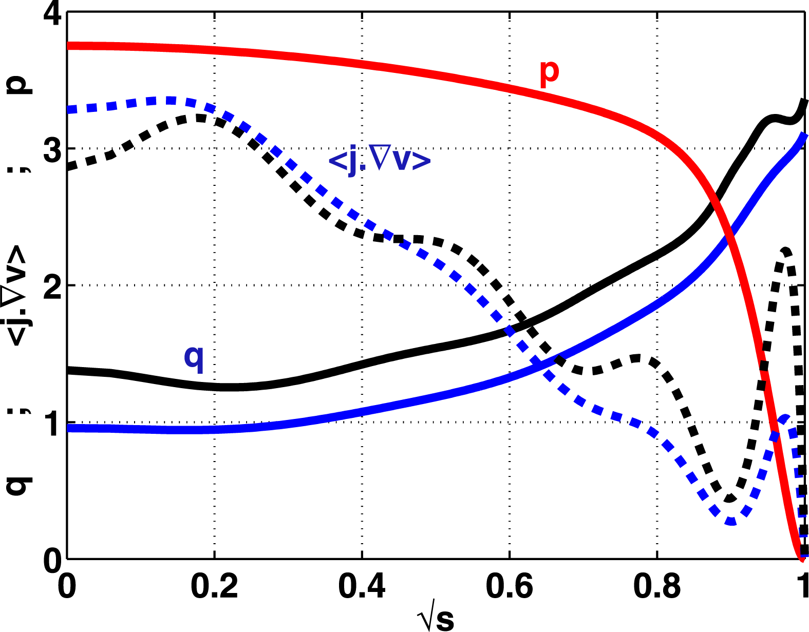Here $J_{BS}$ identifies the total bootstrap current. These profiles are displayed in figure 1 together with the corresponding $q$ -profiles. The small edge bootstrap current case has a core region with $q<1$ ; the large edge bootstrap current case has $q>1$ everywhere and a region of vanishing magnetic shear near the edge of the plasma where $J_{BS}$ has its peak value.

Figure 1.

The pressure profile $p$ (upper solid red line), the toroidal current profiles $\langle \boldsymbol{j}\boldsymbol{\cdot }\boldsymbol{{\rm\nabla}}v\rangle$ for a high edge bootstrap current case $J_{BS}/I_{t}=0.566$ (black dashed curve) and a low edge bootstrap current case $J_{BS}/I_{t}=0.307$ (blue dashed curve) and the corresponding $q$ -profiles (lower solid curves) for a TCV configuration with $\langle {\it\beta}\rangle =1.9\,\%$ and toroidal current $I_{t}=375~\text{kA}$ .

The VMEC equilibrium is transformed into Boozer coordinates (Boozer Reference Boozer1980) and we expand the poloidal mode number spectrum in these coordinates to encompass $0\leqslant m\leqslant 36$ to guarantee a satisfactory reconstruction of the axisymmetric equilibrium state. To obtain converged solutions of the eigenvalue ${\it\lambda}$ with TERPSICHORE, we undertake a study where we vary the number of radial mesh intervals from $116$ to $288$ . 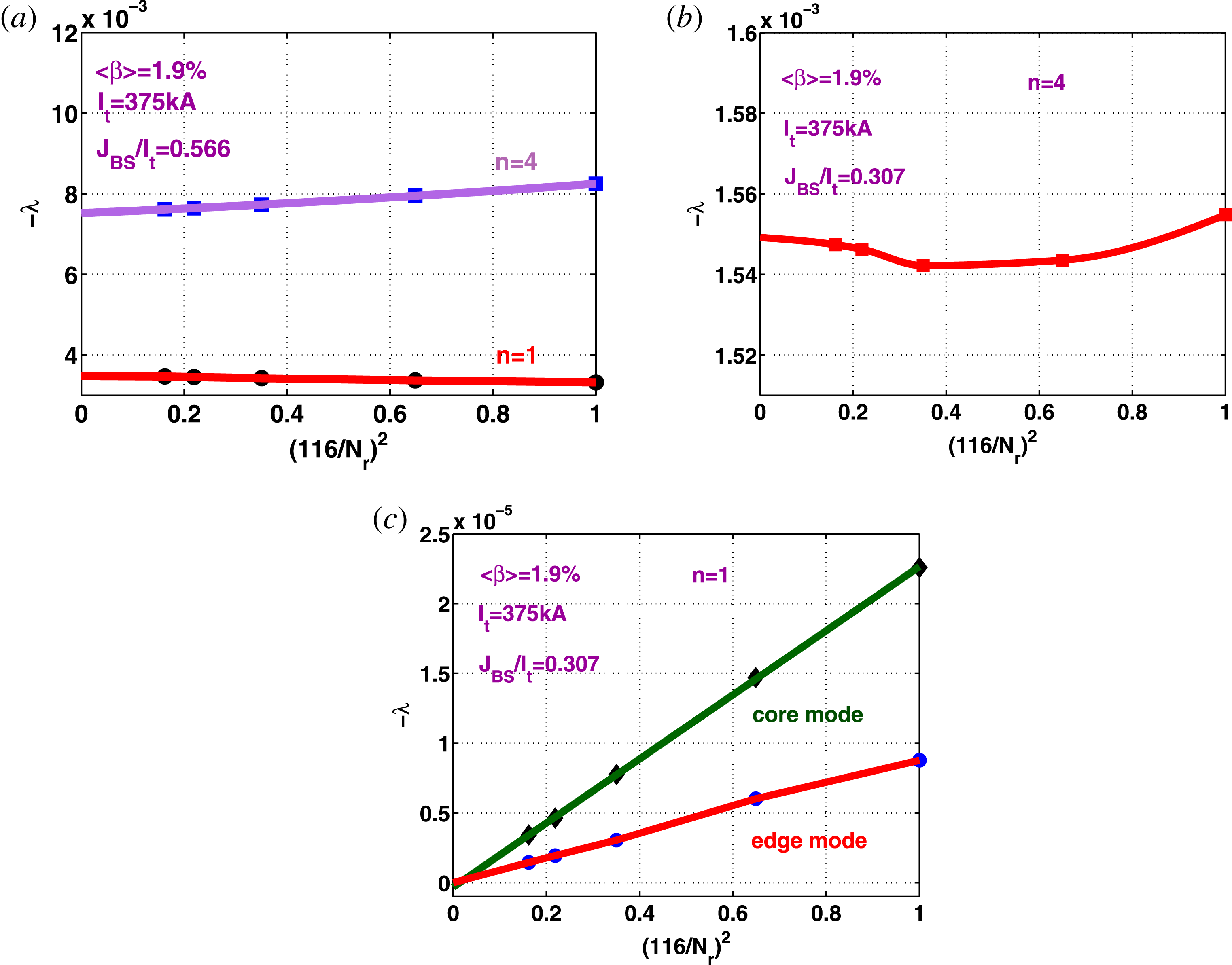The results are presented in figure 2. The linear stability analysis reveals that the $n=1$ mode is unstable and that ${\it\lambda}$ for the $n=4$ mode is twice as big for the large edge bootstrap current case $J_{BS}/I_{t}=0.566$ (figure 2 a). The convergence study for the $n=1$ mode for the small $J_{BS}/I_{t}=0.307$ edge bootstrap current case demonstrates that there is a dominant core $n=1$ mode and a subdominant edge $n=1$ mode, but both of these have ${\it\lambda}\Rightarrow 0$ with infinitesimal mesh size indicating that these structures are in fact stable (figure 2 c). Quadratic convergence is mostly observed for the behaviour of ${\it\lambda}$ with mesh size. 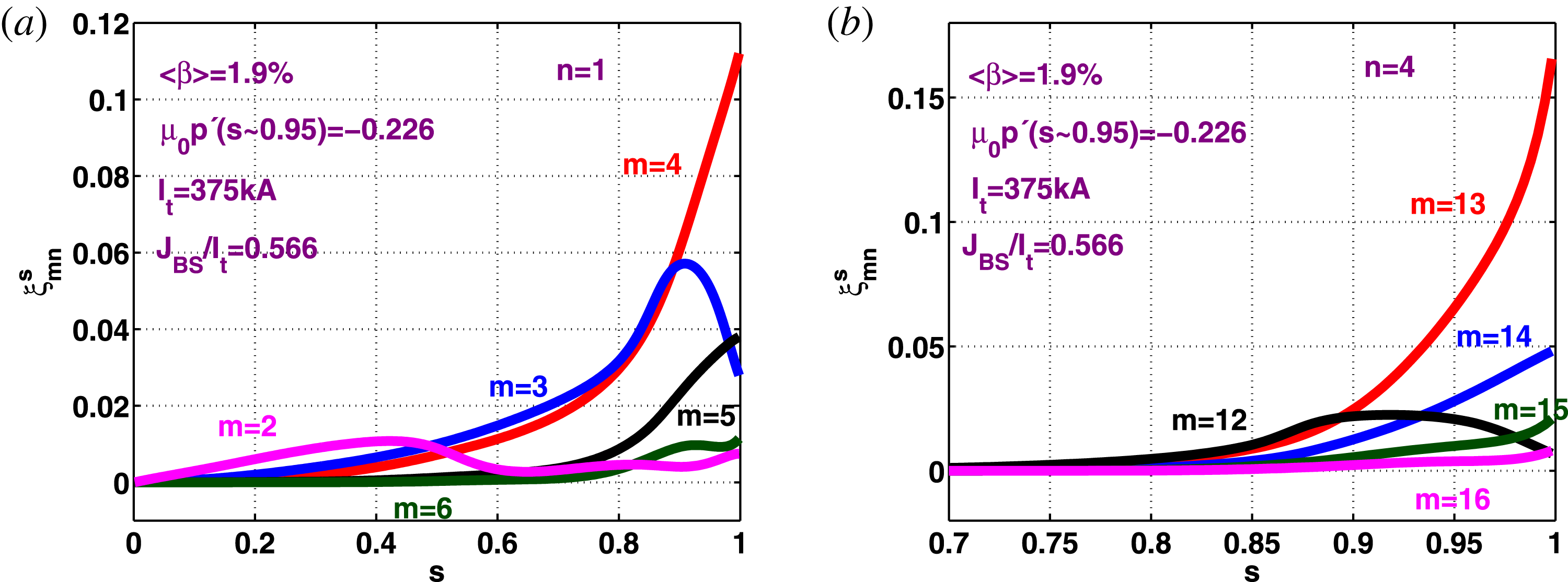The exception to this rule corresponds to the $n=4$ mode for the low $J_{BS}/I_{t}=0.307$ edge bootstrap current case which is unstable and oscillates slightly with a refined mesh (figure 2 b). The five dominant $n=1$ Fourier components of the radial displacement vector ${\it\xi}^{s}={\bf\xi}\boldsymbol{\cdot }\boldsymbol{{\rm\nabla}}s$ for the large edge bootstrap current case ( $J_{BS}/I_{t}=0.566$ ) and the five principal $n=4$ Fourier amplitudes of ${\it\xi}^{s}$ for the small edge bootstrap current case ( $J_{BS}/I_{t}=0.307$ ) as a function of $s$ are displayed in figure 3 and show well resolved mode structures. In the linear phase, the $m/n=4/1$ structure is dominant for $J_{BS}/I_{t}=0.566$ and the $m/n=13/4$ term dominates for $J_{BS}/I_{t}=0.307$ .

Figure 2.

Convergence with the number of radial intervals $N_{r}$ of the unstable eigenvalue ${\it\lambda}$ computed with the TERPSICHORE code of axisymmetric VMEC equilibria with respect to the $n=1$ and $n=4$ toroidal mode number when the bootstrap current to total current ratio $J_{BS}/I_{t}=0.566$ (a), with respect to the $n=4$ mode for $J_{BS}/I_{t}=0.307$ (b) and for the most unstable core $n=1$ eigenmode and a secondary edge $n=1$ eigenmode for $J_{BS}/I_{t}=0.307$ showing that both these are actually linearly stable (c).

Figure 3.

The profiles of the five principal perturbed radial displacement vector Fourier components ${\it\xi}_{mn}^{s}$ of the most unstable $n=1$ eigenmode of the axisymmetric VMEC equilibrium with $J_{BS}/I_{t}=0.566$ (a) and of the most unstable $n=4$ eigenmode with $J_{BS}/I_{t}=0.307$ (b). Note that the mode profiles for $n=4$ are limited to the outer $30\,\%$ of the plasma volume.

4. 3-D equilibrium numerical simulations: nonlinearly stable states

The MHD equilibria of configurations that model the TCV tokamak under free boundary conditions are computed with the VMEC code that assumes that in 3-D, the magnetic flux surfaces are nested and only a single magnetic axis exists. We expand the spectrum of toroidal mode numbers employed in the previous section to encompass $-6\leqslant n\leqslant 6$ Fourier components to describe the system. We then explore the conditions under which 3-D deformations spontaneously develop that break axisymmetry. At low $\langle {\it\beta}\rangle =0.76\,\%$ , the $n\neq 0$ distortions are tiny, but as the we increase $\langle {\it\beta}\rangle$ when the edge bootstrap current is large, spontaneous dominantly $n=1$ 3-D corrugations appear near the boundary region of the plasma. We interpret these deformations as indicative of the development of an external kink/peeling mode that saturates at finite amplitude. The distortions observed are symptomatic of the edge harmonic oscillation (EHO) (Burrell et al. Reference Burrell, West, Doyle, Austin, Casper, Gohil, Greenfield, Groebner, Hyatt and Jayakumar2005) first reported on DIII-D, but subsequently observed on many other machines (Suttrop et al. Reference Suttrop, Hynönen, Kurki-Suonio, Lang, Maraschek, Neu, Stbler, Conway, Hacquin and Kempenaars2005; Hu et al. Reference Hu, Sun, Guo, Li, Wan, Wang, Ding, Xu, Liang and Mansfield2015), and the outer mode (OM) measured on JET (Solano et al. 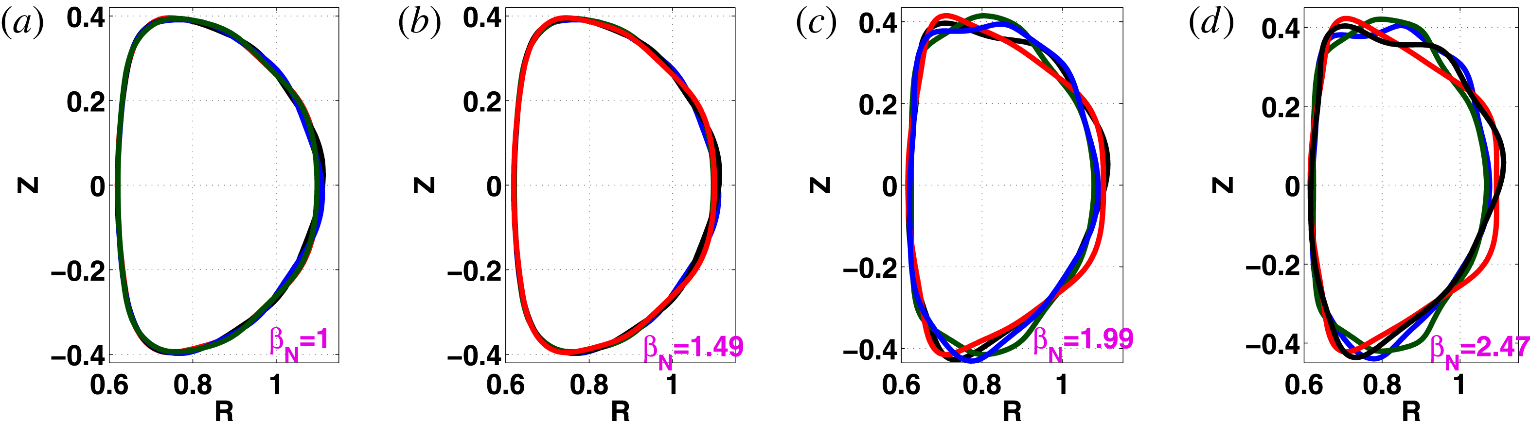Reference Solano, Lomas, Alper, Xu, Andrew, Arnoux, Boboc, Barrera, Belo and Beurskens2010). The shape of the last closed magnetic flux surface on TCV at four different cross-sections projected onto a single toroidal plane for ${\it\beta}_{N}=1$ , $1.49$ , $1.99$ and $2.47$ are presented in figure 4. Distortions of the plasma edge surface become noticeable at ${\it\beta}_{N}=1.49$ and very pronounced at ${\it\beta}_{N}=2.47$ .

Figure 4.

The shape of the last closed TCV magnetic flux surface on four different cross-sections spanning half a toroidal transit projected onto a single plane for $\langle {\it\beta}\rangle =0.76\,\%$ (a), $\langle {\it\beta}\rangle =1.14\,\%$ (b), $\langle {\it\beta}\rangle =1.52\,\%$ (c) and $\langle {\it\beta}\rangle =1.89\,\%$ (d) for the configuration with large edge ( $p^{\prime }<0;J_{BS}>0$ ). The corresponding values for ${\it\beta}_{N}$ are $1$ , $1.49$ , $1.99$ and $2.47$ , respectively. The distortion of the plasma boundary driven by a saturated external kink occurs between ${\it\beta}_{N}=1.49$ and ${\it\beta}_{N}=1.99$ . In this sequence $I_{t}=340~\text{kA}$ .

The two TCV configurations discussed in the previous section are recalculated with the expanded $-6\leqslant n\leqslant 6$ toroidal mode spectrum to investigate deformations that can be triggered in the boundary region of the plasma at $\langle {\it\beta}\rangle =1.9\,\%$ ( ${\it\beta}_{N}=2.25$ ). The thermal pressure distribution at four equidistant toroidal angle planes spanning half a toroidal transit are presented in figure 5(a–d) for the low $J_{BS}/I_{t}=0.307$ edge bootstrap current case that shows a dominant $n=4$ edge corrugation and for the large $J_{BS}/I_{t}=0.566$ edge bootstrap current case which displays dominant $n=1$ distortions in figure 5(e–h).

Figure 5.

The thermal pressure contours at toroidal angle cross-sections $v=0$ (a,e), $v={\rm\pi}/3$ (b,f), $v=2{\rm\pi}/3$ (c,g) and $v={\rm\pi}$ (d,h) for the TCV case with small edge bootstrap current $J_{BS}/I_{t}=0.307$ (a–d) and the pressure contours at the same cross-sections for the TCV case with large edge bootstrap current $J_{BS}/I_{t}=0.566$ (e–h) at $\langle {\it\beta}\rangle =1.9\,\%$ , ${\it\beta}_{N}\sim 2.25$ and $I_{t}=375~\text{kA}$ . The edge region displays the characteristics of an kink/peeling/ballooning mode with a dominant $m/n=6/4$ and subdominant $m/n=7/4,4/4$ and $9/4$ perturbed structure for the low bootstrap current case and the characteristics of an OM with a dominant $m/n=2/1$ and subdominant $m/n=4/1,1/1,0/1$ and $5/1$ perturbed structures for the high bootstrap current case.

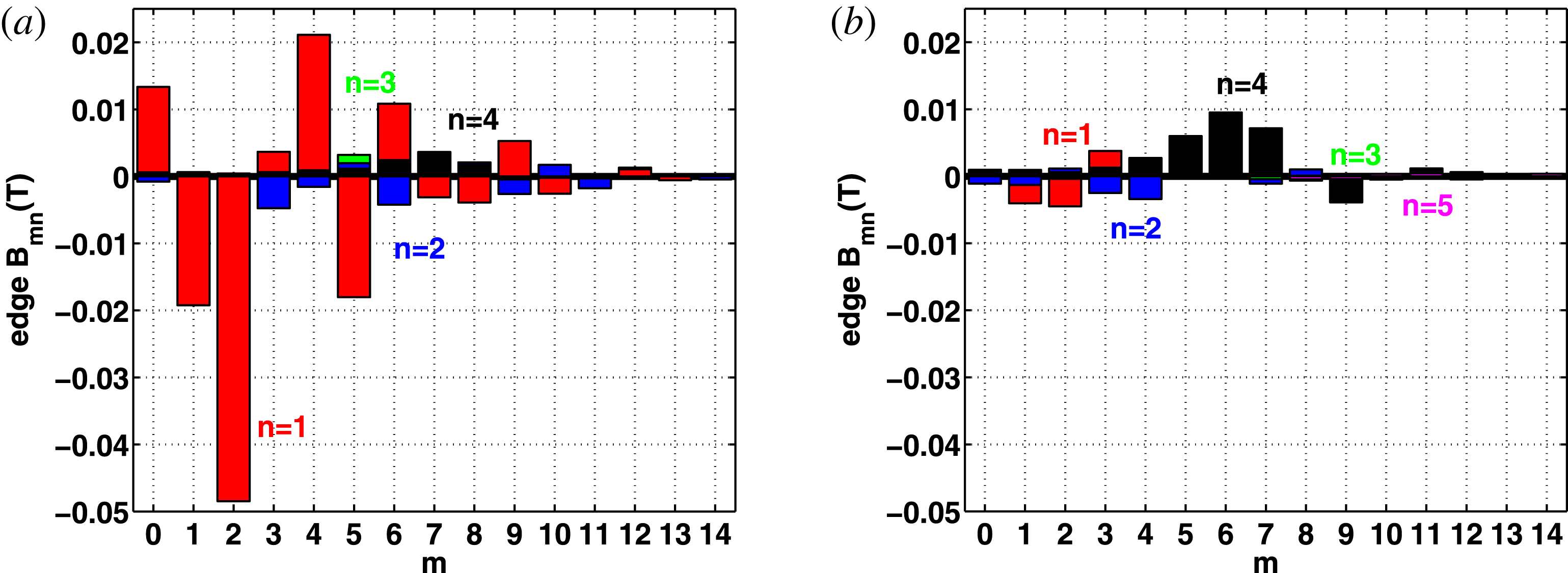
A Fourier analysis of the spectrum of the magnetic field strength $B$ at the last closed magnetic flux surface is presented in figure 6, where we plot $B_{mn}(s=1)$ versus the poloidal mode number $m$ for toroidal mode numbers $n=1$ , $2$ , $3$ , $4$ and $5$ to identify the dominant components of this spectrum. The large $J_{BS}/I_{t}=0.566$ edge bootstrap current case is shown on the left-hand side of figure 6 from which we extract that the $m/n=2/1$ Fourier amplitude of $B$ is dominant with subdominant $m/n=4/1$ , $1/1$ , $5/1$ and $0/1$ structures. The Fourier components of $B$ with $n=2$ , $3$ and $4$ are an order of magnitude smaller than the $B_{21}$ term. The closest resonance surface corresponds to $q=3$ , but we find that the $B_{21}$ and $B_{41}$ non-resonant sidebands are much more important then the resonant $B_{31}$ term in the nonlinear stage. There is consistency with the experimental observations of ELM activity in TCV where unstable $n\sim 15$ modes computed in the linear phase are suppressed in the nonlinear phase so that $n\simeq 1$ structures become dominant (Wenninger et al. Reference Wenninger, Reimerdes, Sauter and Zohm2013) that are further buttressed with linear to nonlinear simulations undertaken with the JOREK code (Krebs et al. Reference Krebs, Hölzl, Lackner and Günter2013; Liu et al. Reference Liu, Huijsmans, Loarte, Garofalo, Solomon, Snyder, Hoelzl and Zheng2015). On the right-hand side of figure 6, we see that for the smaller $J_{BS}/I_{t}=0.307$ edge bootstrap current case, the $m/n=6/4$ Fourier component of $B$ is dominant at the plasma boundary, with subdominant $m/n=7/4$ , $5/4$ and $9/4$ structures also appearing. Again, these components are non-resonant at the edge of the plasma and the $m/n=12/4$ component of $B$ which is closest to the $q=3$ rational surface is negligible.

Figure 6.

The dominant Fourier amplitudes of the magnetic field $B$ components that break axisymmetry $(n\neq 0)$ at the last closed magnetic flux surface as a function of the poloidal mode number $m$ for toroidal mode numbers $n=1,2,3$ and $4$ in TCV for the low edge bootstrap current case $J_{BS}/I_{t}=0.566$ (a) and the high edge bootstrap current case $J_{BS}/I_{t}=0.307$ (b).

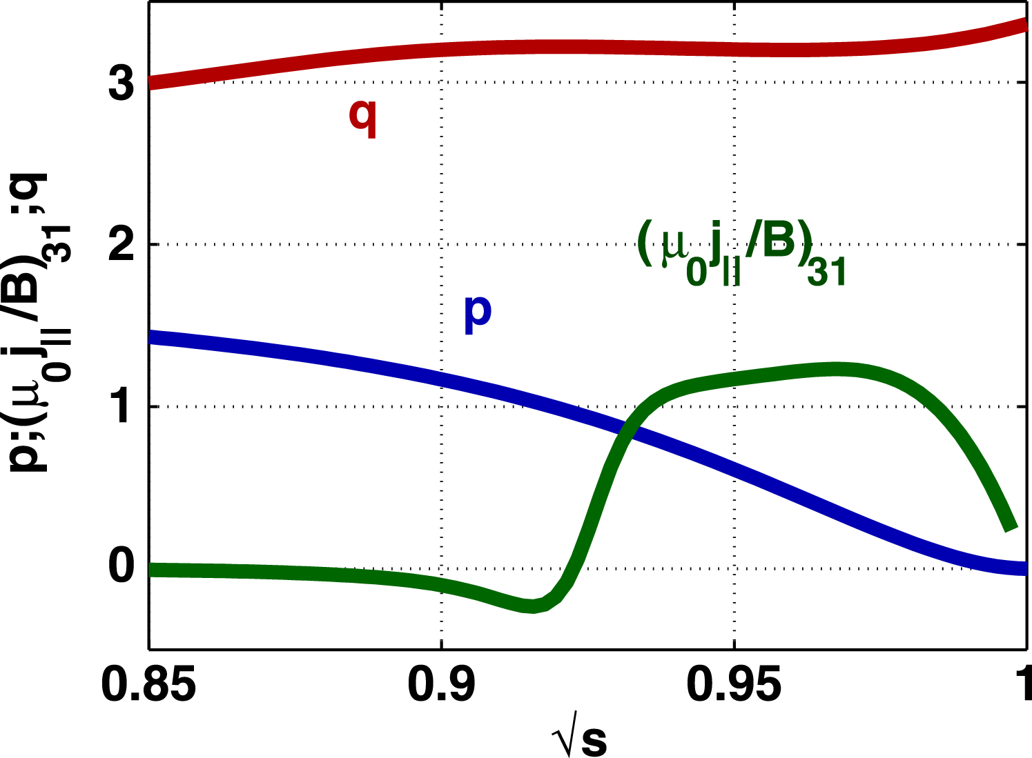
The OM in the JET tokamak is represented by a field-aligned helical current ribbon located at the flat-top of the density pedestal. We examine the behaviour of the equilibrium parallel current density for the large $J_{BS}/I_{t}=0.566$ example we have and find that in the edge region of the plasma, a $m/n=3/1$ Fourier component of ${\it\mu}_{0}j_{\Vert }/B$ becomes large with a significant radial extent that constitutes a helical ribbon similar to that reported on JET. This is shown in figure 7, where we plot the $m/n=3/1$ Fourier amplitude profile of ${\it\mu}_{0}j_{\Vert }/B$ together with the pressure and $q$ -profiles as a function of $\sqrt{s}$ in the outer $15\,\%$ of the plasma radius. The radial extent parallel current ribbon aligns with that corresponding to the region where the magnetic shear vanishes. The parallel current density is driven through charge conservation and MHD force balance by the pressure gradient and represents a Pfirsch–Schlüter current associated with the 3-D distortion of the edge region of the plasma.

Figure 7.

The $q$ , pressure $p$ and the $m/n=3/1$ Fourier component of the parallel current density term ${\it\mu}_{0}j_{\Vert }/B$ profiles at the outer edge of the plasma. The $m/n=3/1$ current ribbon is localised just outside the $q=3$ surface in the region of vanishing magnetic shear. The case in this figure corresponds to $I_{t}=375~\text{kA}$ , $\langle {\it\beta}\rangle =1.9\,\%$ , $J_{BS}/I_{t}=0.566$ and ${\it\mu}_{0}p^{\prime }(s=0.948)=-0.226$ .

In our opinion, the high $J_{BS}/I_{t}=0.566$ case we have presented constitutes an example of a saturated ideal kink/peeling mode while that with the low $J_{BS}/I_{t}=0.307$ case is indicative that the configuration is more likely susceptible to higher $n$ peeling/ballooning modes that cannot be fully resolved with the spectrum of Fourier modes we have applied for the VMEC equilibrium computations we have undertaken. Convergence of an equilibrium with a more extensive Fourier set and correspondingly finer resolution becomes difficult to achieve with VMEC.

In figure 8, we present the contours of the dominant $n=1$ Fourier terms (the poloidal mode number is generally $m=2$ , but can vary in the figure) of $B$ in the domain of the total edge bootstrap current to the total current ratio $J_{BS}/I_{t}$ versus the edge pressure gradient at the $s=0.948$ radial location (which coincides with the position of the peak of the edge bootstrap current profile). For this plot, we employed for simplicity a reduced poloidal mode number spectrum $0\leqslant m\leqslant 10$ . We were unable to converge VMEC equilibria in the domain at the upper edge of the graph for $J_{BS}/I_{t}>0.8$ and at the left-hand side edge of the graph. We surmise that the MHD instability conditions are so adverse that nonlinearly saturated states become unachievable beyond the limits where we have obtained spontaneous 3-D solutions with VMEC. The domain with large $p^{\prime }$ and low $J_{BS}/I_{t}$ is likely to be susceptible to high $n$ peeling/ballooning modes that we are not able to resolve with the spectrum of modes applied in VMEC.

Figure 8.

Contours of the dominant $n=1$ Fourier amplitude of $B_{mn}$ at the last closed magnetic flux surface as a function of the pressure gradient ${\it\mu}_{0}p^{\prime }$ at the surface $s=0.948$ and the ratio of the edge bootstrap current to the total current $J_{BS}/I_{t}$ for a TCV configuration with $\langle {\it\beta}\rangle =1.9\,\%$ and toroidal current $I_{t}=375~\text{kA}$ .

5. Analysis of the linear 3-D ideal MHD analysis

The driving term of the potential energy principle displayed in (3.1) can be written (Dewar et al. Reference Dewar, Monticello and Sy1984; Greene Reference Greene1996; Cooper Reference Cooper1997)

where $D_{B}=2p^{\prime }(s){\bf\kappa}\boldsymbol{\cdot }\boldsymbol{{\rm\nabla}}s$ represents the interaction of the pressure gradient with the normal component of the magnetic field line curvature, $D_{S}={\it\sigma}S|\boldsymbol{{\rm\nabla}}s|^{2}$ describes the interaction of the parallel current density with the local magnetic shear and $D_{J}={\it\sigma}^{2}B^{2}$ is the parallel current density drive. Specifically, the magnetic field line curvature is ${\bf\kappa}=(\boldsymbol{b}\boldsymbol{\cdot }\boldsymbol{{\rm\nabla}})\boldsymbol{b}$ , where $\boldsymbol{b}=B/B$ is the unit vector along the magnetic field lines, while the local magnetic shear is defined as $S=-\boldsymbol{h}\boldsymbol{\cdot }\boldsymbol{{\rm\nabla}}\times \boldsymbol{h}$ with $\boldsymbol{h}=B\times \boldsymbol{{\rm\nabla}}s/|\boldsymbol{{\rm\nabla}}s|^{2}$ (Greene & Johnson Reference Greene and Johnson1968; Dewar et al. Reference Dewar, Monticello and Sy1984; Hegna Reference Hegna2000). The parallel current density factor is ${\it\sigma}\equiv \boldsymbol{j}\boldsymbol{\cdot }B/B^{2}$ and ${\bf\xi}$ is the perturbed displacement vector.

We do not carry out linear ideal MHD stability calculations for the eigenvalue and eigenfunction, but instead apply the diagnostic routines of the TERPSICHORE code (Anderson et al. Reference Anderson, Cooper, Gruber, Merazzi and Schwenn1990; Cooper Reference Cooper1992) to evaluate the instability drive terms (Cooper Reference Cooper1997) in Boozer magnetic coordinates (Boozer Reference Boozer1980), where we label the poloidal angle ${\it\theta}$ and the toroidal angle ${\it\phi}$ . The rationale for this approach is based on the fact that all low $n$ structures have already been included in the VMEC equilibrium calculation to achieve a minimum energy state within the bounds of the mode spectrum $0\leqslant m\leqslant 14$ ; $-6\leqslant n\leqslant 6$ . It would only make sense to investigate linear ideal MHD stability with respect to modes that have been excluded from this spectrum. The interactions of $\sqrt{g}D_{B}=2\sqrt{g}p^{\prime }(s){\bf\kappa}\boldsymbol{\cdot }\boldsymbol{{\rm\nabla}}s$ , $\sqrt{g}D_{J}=\sqrt{g}j_{\Vert }^{2}$ and $\sqrt{g}D_{S}=\sqrt{g}{\it\sigma}S|\boldsymbol{{\rm\nabla}}s|^{2}$ from left to right for the large $J_{BS}/I_{t}=0.566$ , respectively, on an unwrapped toroidal magnetic flux contour with $s\sim 0.925$ near the edge of the plasma in TCV appears in figure 9(a–c). Here $\sqrt{g}$ is the Jacobian of the transformation from the Boozer coordinates to the Cartesian frame. We see that $\sqrt{g}j_{\Vert }^{2}$ is the largest destabilising term with a clear $n=1$ structure localised at the outer midplane of the plasma ( ${\it\theta}=0,2{\rm\pi}$ ). This is significantly counteracted by the interaction of $j_{\Vert }$ with the local magnetic shear which is mostly stabilising, particularly at the outer midplane. The interaction of $p^{\prime }$ with the normal curvature also displays a destabilising $n=1$ structure, but is almost an order of magnitude smaller than the $\sqrt{g}j_{\Vert }^{2}$ contribution. Hence, the dominance of the $n=1$ mode that drives linear ideal instability is consistent with the nonlinearly saturated kink/peeling structure obtained with the VMEC calculation. In figure 9(d–f) we present the distributions of $\sqrt{g}D_{B}$ , $\sqrt{g}D_{J}$ and $\sqrt{g}D_{S}$ on the poloidally and toroidally unwrapped magnetic surface at $s=0.925$ for the TCV equilibrium with low $J_{BS}/I_{t}=0.307$ edge bootstrap current from left to right, respectively. In this case, the structures of the linear instability driving terms are all dominated by $n=4$ modes, consistent again with the nonlinearly saturated state calculated with the VMEC equilibrium solver. The dominant instability drive is $\sqrt{g}j_{\Vert }^{2}$ , but it is also counteracted by the stabilising impact of $\sqrt{g}D_{S}=\sqrt{g}{\it\sigma}S|\boldsymbol{{\rm\nabla}}s|^{2}$ specially at the outer midplane. The interaction of $p^{\prime }$ with the normal curvature for low $J_{BS}/I_{t}=0.307$ is approximately twice as large as that for $J_{BS}/I_{t}=0.566$ . This insinuates that peeling/ballooning structures which are not fully resolved with the equilibrium mode spectrum we have retained could have an important bearing for cases with large $p^{\prime }$ and small $J_{BS}/I_{t}$ , corresponding to the domain at the bottom right edge of the scan presented in figure 8. The OM/EHO emerge at the top edge in figure 8, which are very well resolved in our VMEC computations.

Figure 9.

The interaction of the pressure gradient with the magnetic field line curvature $2\sqrt{g}p^{\prime }(s){\bf\kappa}\boldsymbol{\cdot }\boldsymbol{{\rm\nabla}}s$ (a,d), the parallel current density drive $\sqrt{g}{\it\sigma}^{2}B^{2}=\sqrt{g}j_{\Vert }^{2}$ (b,e) and the interaction of the parallel current density with the local magnetic shear $\sqrt{g}{\it\sigma}S|\boldsymbol{{\rm\nabla}}s|^{2}$ (c,f) in a TCV configuration with high edge bootstrap current $J_{BS}/I_{t}=0.566$ (a–c) in a TCV configuration with low edge bootstrap current $J_{BS}/I_{t}=0.307$ (d–f) on a poloidally and toroidally unwrapped flux surface at the position $s=0.925$ , where ${\it\theta}$ and ${\it\phi}$ are the Boozer poloidal and toroidal angles, respectively. The pressure gradient at $s=0.925$ for both configurations is ${\it\mu}_{0}p^{\prime }=-0.226$ , $I_{t}=375~\text{kA}$ and $\langle {\it\beta}\rangle =1.9\,\%$ .

6. Summary and conclusions

The main conclusion of the work we have presented relates to novel free boundary tokamak equilibria with spontaneously developed unprompted 3-D distortions to the plasma–vacuum interface when $\langle {\it\beta}\rangle$ exceeds a threshold value using the VMEC code. We predict the corrugations to occur for $\langle {\it\beta}\rangle >1.5\,\%$ in the TCV tokamak. The solutions with 3-D deformations resemble saturated ideal kink/peeling instability structures. As a prelude to the unconventional 3-D MHD equilibrium solutions we have obtained, ideal MHD stability calculations of axisymmetric TCV tokamak equilibria reveal that $n=1$ internal modes are linearly unstable for large edge bootstrap currents and that higher $n$ mode structures are more unstable than for $n=1$ . For low edge bootstrap currents, the core and edge $n=1$ modes are stable. We find, that $n=4$ external modes become unstable. However, we contend that the magnitudes of linear ideal MHD growth rates are deceptive. Although the linear phase indicates that large $n$ toroidal mode numbers are important, the nonlinear phase exhibits a dominance of $n=1$ corrugations particularly when the edge $J_{BS}$ becomes large. This is consistent with observations of ELM behaviour in the TCV tokamak, which reports the dominance of $n=1$ toroidal structures (Wenninger et al. Reference Wenninger, Reimerdes, Sauter and Zohm2013), as well as numerical simulations with the JOREK code that shows $n=1$ modes becoming increasingly important from the linear to the early nonlinear phases (Krebs et al. Reference Krebs, Hölzl, Lackner and Günter2013) and then completely dominant in the saturated nonlinear phase (Liu et al. Reference Liu, Huijsmans, Loarte, Garofalo, Solomon, Snyder, Hoelzl and Zheng2015). For small edge $J_{BS}$ and large edge $p^{\prime }$ , larger $n$ peeling/ballooning modes become relevant, but we are cannot fully resolve these with the spectrum of modes applied to converge 3-D equilibrium states with the VMEC code. We have concentrated our efforts in the domain where $J_{BS}$ at the edge is large, which tends to coincide with the region where low $n=1$ structures dominate (corresponding to the upper half of the graph in figure 8). In our opinion, these structures constitute a very realistic model for the OM observed on JET (Solano 2010) and the EHO detected on DIII-D and other tokamaks (Burrell et al. Reference Burrell, West, Doyle, Austin, Casper, Gohil, Greenfield, Groebner, Hyatt and Jayakumar2005; Suttrop et al. Reference Suttrop, Hynönen, Kurki-Suonio, Lang, Maraschek, Neu, Stbler, Conway, Hacquin and Kempenaars2005; Hu et al. Reference Hu, Sun, Guo, Li, Wan, Wang, Ding, Xu, Liang and Mansfield2015). A detailed analysis of the equilibrium state for large edge $J_{BS}$ indicates that a parallel helical current density ribbon forms just outside the $q=3$ rational surface with a radial extent that aligns with the vanishing magnetic shear region associated with the flat spot in the $q$ -profile caused by the bootstrap current. Fourier analysis demonstrates that this parallel current ribbon corresponds to a near resonant $m/n=3/1$ helical structure. The spectrum of the magnetic field strength $B$ at the edge of plasma, however, has a very weak resonant component, but significant $m/n=2/1$ and $m/n=4/1$ non-resonant terms. The mechanism for the development of the current ribbon corresponds to the non-axisymmetric component of the Pfirsch–Schlüter current that results from the 3-D deformation of the plasma boundary region. The linear stability analysis of the 3-D TCV tokamak equilibria confirms the dominance of $n=1$ structures for large edge $J_{BS}$ and shows that $n=4$ corrugations are most relevant for low $J_{BS}$ , possibly insinuating susceptibility to peeling/ballooning modes in this case.

The nonlinearly saturated 3-D equilibrium states we have obtained constitute a solid platform to investigate a wide range of tokamak physics phenomena associated with quiescent H-mode tokamak plasmas with quasicoherent OM and EHO structures (such as fast particle confinement or turbulence). The economic feasibility of tokamak reactors will inevitably require H-mode plasmas. However, this mode is unsustainable if ELM are triggered.