1 Introduction
Partial observability is a challenging characteristic of the environments that reinforcement learning (RL) algorithms operate on (Sutton & Barto, Reference Sutton and Barto1998). As the states of the environment are not directly available, the learning agent has to cope with partial and possibly ambiguous observations in order to learn the dynamics of the underlying environment. Such a task is especially difficult when multiple states map to the same observation, causing a fundamental problem called perceptual aliasing (Whitehead & Ballard, Reference Whitehead and Ballard1991; Chrisman, Reference Chrisman1992). Depending on the degree of ambiguity on the observations, finding the optimal action for each state may not be possible.
Landmarks, on the other hand, provide sufficient information to distinguish a problem state, so that they can help the agent in the learning phase. Providing a reliable knowledge, landmarks can guide an agent in the learning task and hence speed up the learning (James & Singh, Reference James and Singh2009). Although their presence is used in the literature, automatic identification of landmarks is left unexplored.
In robotics, a landmark may correspond to a location or an object that is unique in that environment. It may provide some insight into the robot about its progress and guide it to complete the given task. Under partial observability, the robot may benefit from the landmarks in order to locate itself in the environment. Thus, discovery of the landmarks of an environment may be useful for planning in robotics domain, especially for navigational tasks.
Making use of landmarks has been shown to improve learning performance for memoryless RL agents in partially observable environments. We refer to this class of tasks as Landmark-POMDPs. SarsaLandmark (James & Singh, Reference James and Singh2009) enhances the classical Sarsa(λ) algorithm (Loch & Singh, Reference Loch and Singh1998) by skipping the non-landmark states in the eligibility trace mechanism, so that a higher-level tracking of reliable observations (i.e., landmarks) is promoted. However, SarsaLandmark assumes that the agent knows in advance all of the landmark states, which is not a realistic scenario both in real life and in terms of ‘learn-from-scratch’ philosophy of RL. In this paper, we propose an RL framework to extend SarsaLandmark with automatic landmark identification capability. For this purpose, we utilize a statistical method based on multiple instance learning, named Diverse Density (DD) (McGovern & Barto, Reference McGovern and Barto2001). DD classifies instances based on raw experiences and ignores the direct features of the states/observations, which makes it ideal for landmark identification since the state space is hidden from the agent. The resulting framework succeeds to automatically identify landmarks during learning, feed the identified landmarks to SarsaLandmark, and achieves much the same learning performance with SarsaLandmark.
A side contribution of the paper is that it provides a deeper analysis on DD with Concept Filtering (DDCF), which we briefly introduced for another problem setting recently (Demir et al., Reference Demir, Çilden and Polat2017), aiming to enhance DD by means of a Concept Filtering heuristic. With DDCF, McGovern’s original DD algorithm (MDD) (McGovern & Barto, Reference McGovern and Barto2001) is significantly improved, in terms of both time and quality. We also show that DDCF can effectively be incorporated within the proposed framework.
The organization of the paper is as follows: Section 2 provides a summary of background necessary to track the concepts throughout the paper. DDCF and the proposed framework are incrementally presented in Section 3. The settings and results of an extensive experimentation on the subject are given in Section 4, together with a discussion. Section 5 concludes the paper and suggests possible future work.
2 Background and related work
This section provides a brief introduction to the POMDP model, an on-policy learning algorithm Sarsa(λ), and discusses the related work on automatic abstraction in RL with emphasis on subgoal discovery techniques, by which this study is inspired.
2.1 POMDPs
A POMDP is defined by the tuple  $\left\langle S,A,T,R,\Omega,O \right\rangle $, where S is a finite set of states, A is a finite set of actions, and
 $T : S\times A \times S \rightarrow [0, 1]$ is the transition function where T(s, a, s’) is the probability of being in state s’ if action a is performed in state s and
 $\forall s \in S$,
 $\forall a \in A$,
 $\sum_{s' \in S} T\left( s, a, s'\right) = 1$.
 $R : S \times A \rightarrow \Re$ is the reward function where R(s, a) gives the immediate reward from the environment after taking action a in state s.
 $\Omega$ is a finite set of observations through which the agent can experience its surroundings, and
 $O:S \times A \rightarrow \Pi(\Omega)$ is the observation function which gives, for each action and resulting state, a probability distribution over possible observations. O(s’, a, o) denotes the probability of making observation o given that the agent took action a and landed in state s’ (Kaelbling et al., Reference Kaelbling, Littman and Cassandra1998).
When observations are the only sources of information about the environment, a challenging problem for RL arises, called perceptual aliasing. If the same observation is obtained by the agent in two distinct states (for which optimal actions are probably different), the states are said to be perceptually aliased (Whitehead & Ballard, Reference Whitehead and Ballard1991; Chrisman, Reference Chrisman1992).
2.2 Sarsa(λ)
Sarsa(λ) is a family of on-policy learning algorithms that uses the notion of eligibility traces (Loch & Singh, Reference Loch and Singh1998). The key idea behind this approach is that it updates the regular Q values of observation-action pairs with an error while leaving a trace over the previously visited observation-action pairs. After the agent experiences the transition  $\langle o_{t}, a_{t}, r_{t}, o_{t+1} \rangle$ at time step t in which the agent gathers observation
 $o_{t+1}$ and receives reward
 $r_{t}$ by taking action
 $a_{t}$ on the observation
 $o_{t}$, the following update rules are employed in the corresponding order:
 $$\eta_{t}(o_{t}, a_{t}) = 1$$
 $$\forall(o \neq o_{t} \text{ or } a \neq a_{t}), \quad \eta_{t}(o, a) = \gamma \cdot \lambda \cdot \eta_{t-1}(o, a)$$
 $$ \forall o, a, \quad Q_{t+1}(o, a) = Q_{t}(o, a) + \alpha \cdot \eta_{t}(o, a) \cdot \delta_{t}$$
where  $\eta_{t}(o, a)$ is the eligibility trace of the observation-action pair
 $\langle o,a \rangle$ at time step t, α is the step size, λ is the trace decay constant, and
 $\delta_{t} = r_{t} + \gamma \cdot Q_{t}(o_{t+1}, a_{t+1}) - Q_{t}(o_{t}, a_{t})$ is the Temporal Difference error (TD-error) at time step t.
By means of the parameter  $0 \leq \lambda \leq 1$, the algorithm maintains a decay over the eligibility traces, together with a reset operation at the end of each episode. Sarsa(λ) is shown to converge to a good policy, even if there is no memoryless solution to the problem (Loch & Singh, Reference Loch and Singh1998).
2.3 Automatic abstraction in reinforcement learning
The famous ‘divide-and-conquer’ strategy has been practiced for RL research for a few decades, with a number of studies which show that dividing the problem into sub-problems and making abstractions based on them can significantly improve learning performance (Dietterich, Reference Dietterich2000; Hengst, Reference Hengst2012). However, it is not always straightforward to devise a meaningful partitioning scheme. Thus, an immediate successor of this problem is how to generate or extract the abstraction partitions automatically.
In policy-based approaches, abstractions are generated directly through processing the policy space. Various methods are used in this track, such as Bayesian networks (Jonsson & A. Barto, Reference Jonsson and Barto2006; Mugan & Kuipers, Reference Mugan and Kuipers2009), probabilistic inference (Daniel et al., Reference Daniel, van Hoof, Peters and Neumann2016), decision trees (Uther & Veloso, Reference Uther and Veloso2003), and commonality analysis (Pickett & Barto, Reference Pickett and Barto2002).
On the other hand, another heuristic approach drew significant attention, which is based on identification of subgoals in the state space. Basically, a subgoal is a state that the agent should visit on the way to achieve its goal, and subgoals are usually related to the bottleneck regions of the problem.
If the problem structure is known in advance, subgoal states can effectively be identified using various techniques. Automatic subgoal discovery, on the other hand, aims to identify the subgoals during the learning phase, without a priori knowledge of the underlying problem characteristics. Identification of subgoals in the early stages of learning can enhance performance by means of some abstraction derivation mechanisms, inherently partitioning the problem in hand (McGovern & Barto, Reference McGovern and Barto2001). Most of these mechanisms are based on formal abstraction frameworks such as options framework (Sutton et al., Reference Sutton, Precup and Singh1999).
There are a number of approaches for automatic discovery of subgoals in the fully observable setting. Probably the most straightforward idea is to keep track of the irregularities, or peaks, of the reward signal. The agent marks a state as a subgoal if it gathers a relatively high reward upon reaching it. For obvious reasons, this approach is not suitable for problems with delayed reinforcement (Digney, Reference Digney1998).
Another widely used approach is based on state observation frequencies, where a state with higher visitation score is presumed a stronger candidate as a subgoal than others, and is marked so if it passes a statistical filter (Stolle & Precup, Reference Stolle, Precup, Koenig and Holte2002; Simsek, Reference Simsek2008). This family of methods usually requires problemspecific statistical parameter values and needs extensive exploration of the problem.
Few researchers tried to make use of the information gathered during RL to identify subgoals, like some structural properties or the relative orientation of the reward peak (Goel & Huber, Reference Goel and Huber2003; Xiao et al., Reference Xiao, Li and Shi2014).
In the graph-based methods, on the other hand, the learning agent first constructs a state transition diagram using its experiences. Then, different techniques are incorporated to separate the strongly connected regions from each other, and the states in between are marked as subgoals (Menache et al., Reference Menache, Mannor and Shimkin2002; Mannor et al., Reference Mannor, Menache, Hoze and Klein2004; Simsek et al., Reference Simsek, Wolfe and Barto2005). These methods also require extensive exploration of the domain and are constrained by the limitations of the underlying graph algorithms.
There are few related studies targeting problems with limited observability, and they tend to focus on temporal abstractions (Yoshikawa & Kurihara, Reference Yoshikawa and Kurihara2006) rather than subgoal discovery. In this category, due to perceptual aliasing among the underlying states, subgoals are extremely difficult to identify.
Instead, it is more useful and realistic to assume that naturally, a subgoal yields a unique observation, called a landmark. A learning agent can certainly benefit from distinguishing observations as landmarks, if they are provided in advance (James & Singh, Reference James and Singh2009). We believe that landmarks can be automatically identified during learning, which is the main motivation of this study.
3 SarsaLandmark with automatic landmark identification
In the following subsections, a novel framework that automatically identifies landmarks and uses them in the learning process is incrementally presented. The section starts by explaining the notion of landmarks, the Landmark-POMDP model, SarsaLandmark, and DD. Then, an improvement over DD with a concept filtering mechanism is introduced, which employs two well-known graph-based metrics to form a new one. Finally, a novel framework which fuses SarsaLandmark with automatic landmark discovery is presented.
3.1 Landmarks and landmark-POMDPs
A landmark has its obvious meaning in the real life as ‘a recognizable natural or artificial feature used for navigation, a feature that stands out from its near environment and is often visible from long distances’ (Wikipedia, 2018). In Artificial Intelligence literature, landmark has different formal definitions and meanings.
Planning researchers define landmark states as those that lie on every optimal path to the goal state (Lazanas & Latombe, Reference Lazanas and Latombe1995; Hoffmann et al., Reference Hoffmann, Porteous and Sebastia2004; Elkawkagy et al., Reference Elkawkagy, Bercher, Schattenberg and Biundo2012; Karpas et al., Reference Karpas, Wang, Williams and Haslum2015). This is, in a sense, a strong definition of landmark, restricting any solution to contain the landmark instance. In this setting, landmarks are commonly assumed stationary.
In robotic navigation research, a landmark is usually defined over perceptions as ‘locally distinctive features’, such as walls and doorways. In that sense, since the identification is local, there is no theoretical need for the landmarks to be stationary, although sensor aliasing due to noise is a major problem (Howard & Kitchen, Reference Howard and Kitchen1999; Koenig & Simmons, Reference Koenig and Simmons1998; Frommberger, Reference Frommberger2008; Välimäki & Ritala, Reference Välimäki and Ritala2016).
In RL context, the use of landmarks dates back to mid-2000s, with James and Singh’s studies. They prefer to make a weaker definition of landmark, in terms of state-observation mapping, not restricting its existence in any policy, as in the planning domain (James & Singh, Reference James and Singh2009). Our study is based on a definition of a landmark that has a broader sense, which also covers their definition.
Definition 1. A landmark is a compact information that uniquely maps to a state in a partially observable environment.
In a general sense, the compact information mentioned here can be a sequence of observations and actions mapping to a unique state. However, if a single state s yields only one observation o and the observation o is specific to state s, this definition also holds and the observation o is a landmark.
Focus of this study is on single observation landmarks since they are ‘naturally present in the environment’. Note that, this definition assumes that a landmark state is an integral part of the problem structure, existing in the model without requiring any other information. From this point on, any usage of the term ‘landmark’ will assume a single observation mapping to a single state.
Following the formal definition of a landmark, Landmark-POMDP is a special form of POMDP which contains at least one landmark (James & Singh, Reference James and Singh2009).
3.2 SarsaLandmark
SarsaLandmark (James & Singh, Reference James and Singh2009) is an adaptation of Sarsa(λ) to handle Landmark-POMDPs. The motivation behind SarsaLandmark is that in the presence of landmark states, skipping over non-landmark states during the Q-value updates may help Sarsa(λ) to converge faster. The method incorporates λ = 1 throughout learning, with the exception that whenever a landmark is observed, λ is set to zero. With this adaptation, upon experiencing a transition  $\langle o_{t}, a_{t}, r_{t}, o_{t+1} \rangle$ at time t, the agent executes the following update rules:
 $$\eta_{t}(o_{t}, a_{t}) = 1$$
 $$\forall(o \neq o_{t} \text{ or } a \neq a_{t}), \eta_{t}(o, a) =\begin{cases}0 & \text{if $o_{t}$ is an observation} \\& \text{by a landmark state} \\ \gamma \cdot \eta_{t-1}(o, a) & \text{otherwise}\end{cases}$$
 $$\forall o, a, \quad Q_{t+1}(o, a) = Q_{t}(o, a) + \alpha \cdot \eta_{t}(o, a) \cdot \delta_{t}$$
where the terms are defined as in Sarsa(λ). Note the differences between rules (2) and (5) of the corresponding update sequences, and that λ is ignored in rule (5) since it is ineffective to the result.
SarsaLandmark reduces to Sarsa(0) if every state is a landmark (full observability), while it is equivalent to Sarsa(1) in a partially observable setting with no landmark states. It is shown that SarsaLandmark is an improvement over Sarsa(λ), in terms of fast policy convergence (James & Singh, Reference James and Singh2009). DD is an effective method to attack multiple-instance (MI) problems. DD treats an MI problem so that it consists of positive and negative bags of instances. Each positive bag contains at least one positive instance, and each negative bag contains only negative instances. The aim is to find the target concept by using only the sign tags (positive or negative) of bags, since the instances are not labeled individually.
3.3 Diverse density
DD is an effective method to attack multiple-instance (MI) problems. DD treats an MI problem so that it consists of positive and negative bags of instances. Each positive bag contains at least one positive instance, and each negative bag contains only negative instances. The aim is to find the target concept by using only the sign tags (positive or negative) of bags, since the instances are not labeled individually.
Maron and Lozano-Pèrez (Reference Maron and Lozano-Pérez1998) propose a metric called DD and define the DD of a target concept  $c_{t}$ as:
 $$\begin{equation}DD(c_{t})=Pr(c_{t}|B_1^+,\ldots,B_n^+,B_1^-,\ldots,B_m^-)\end{equation}$$
where  $Pr(c_{t})$ is the probability that
 $t{\rm th}$ concept is the correct concept,
 $B_i^+$ is the
 $i{\rm th}$ positive bag, and
 $B_i^-$ is the
 $i{\rm th}$ negative bag. The target concept is the one with the highest DD value and the search space is
 $$\begin{equation} DD(c_{t}) = \prod_{1 \leq i \leq n} Pr(c_{t}|B_i^+) \prod_{1 \leq i \leq m} Pr(c_{t}|B_i^-).\end{equation}$$
The terms in this equation are defined with a noisy-or model:
 $$\begin{equation} \begin{aligned} Pr(c_{t}|B_i^+) & = 1 - \prod_{j} (1-Pr(B_{ij}^+ \in c_t)) \\ Pr(c_{t}|B_i^-) & = \prod_{j} (1-Pr(B_{ij}^- \in c_t)) \end{aligned} \end{equation}$$
where  $B_{ij}$ is the
 $j{\rm th}$ instance of the
 $i{\rm th}$ bag, and
 $Pr(B_{ij} \in c_t)$ is defined to be a Gaussian probability inversely proportional with the distance from the particular instance to the target concept.
McGovern and Barto (Reference McGovern and Barto2001) model the task of automatic subgoal identification in an Markov Decision Process (MDP) model as a multiple instance problem and adopt DD for the solution. Their approach considers each state gathered from the environment as a concept, presuming every successful episode as a positive bag and all other episodes as negative bags. On this matter, besides being defined as whether the agent reached the goal state or not, the success of an episode may also be dependent on a step threshold, that is, an episode may be required to reach the goal state under a given number of steps in order to be considered as successful.
McGovern and Barto propose that a bottleneck state, possibly a subgoal, must be observed in positive bags but not in negative ones. In that case, a bottleneck state is expected to have a higher DD value as the result of an exhaustive DD search.
3.4 Bridging and clustering coefficients
Bridging Coefficient BC(v) of a vertex v in a graph is a local measure showing how much connection v brings to its neighbors (Hwang et al., (Reference Hwang, Kim, Ramanathan and Zhang2008):
 $$BC(v) = \frac{d^{-1}(v)}{\sum_{v' \in N(v)}{d^{-1}(v')}}$$
where d(v) is the degree of v and N(v) is the set of direct neighbors of v.
Clustering Coefficient CC(v) of a vertex v is also a local measure determining how well v is clustered (Watts & Strogatz, Reference Watts and Strogatz1998). A generalization of CC(v) that extends the neighborhood of v to the neighbors at depth k, called the k-Clustering Coefficient, denoted  $CC^{(k)}(v)$ (Jiang & Claramunt, Reference Jiang and Claramunt2004), and is formulated as:
 $$\begin{equation} CC^{(k)}(v) = \frac{2e^{(k)}}{n^{(k)}(n^{(k)}-1)} \end{equation}$$
where  $e^{(k)}$ is the number of edges among k neighbors of v, and
 $n^{(k)}$ is the number of nodes within k neighborhood of v. Obviously,
 $CC(v)=CC^{(1)}(v)$.
Computing BC(v) and  $CC^{(k)}(v)$ require less time compared to their global counterparts (Hwang et al., Reference Hwang, Kim, Ramanathan and Zhang2008; Yang & Liu, Reference Yang and Liu2008) which span the entire graph of concern. On the other hand, they also have certain disadvantages in terms of solution quality, depending on the structure of the target graph (Demir et al., Reference Demir, Çilden and Polat2017).
3.5 Diverse density with concept filtering
The original version of McGovern’s DD approach (MDD) was proposed in order to discover subgoals in fully observable RL tasks. It is shown that the extensive DD search idea is able to find bottleneck regions of the problem (McGovern & Barto, Reference McGovern and Barto2001). However, some of its drawbacks prevent its applicability to real life problems.
First of all, in order to calculate the DD values of each concept, the method uses a similarity measure between concepts. McGovern and Barto suggest a Gaussian distance measure which depends on the graph distances between the observations (McGovern & Barto, Reference McGovern and Barto2001). The distances are precalculated and are provided to the agent before the learning process starts. However, this means that the agent has a priori knowledge about the structure (or transition dynamics, to be more accurate) of the problem. It is arguable that providing this knowledge in advance conflicts with the ‘learn-from-scratch’ philosophy of RL.
Another drawback of the DD approach is that it takes each and every concept into account for evaluation as a bottleneck candidate. Since an extensive DD search is employed among the bags upon finishing every episode, this computation is very time consuming. However, apparently not all of the observations are eligible for candidacy.
In our previous work (Demir et al., Reference Demir, Çilden and Polat2017), we argue that a concept filtering approach can be exercised to eliminate some of the concepts by examining their features in the interaction graph (G), which is formed by the actual transitions experienced by the agent within the environment.
Definition 2. An interaction graph G is a weighted directed graph where each vertex  $v \in V$ corresponds to an observation obtained from the POMDP model and each edge
 $e=(v,v') \in E$ corresponds to a transition from observation v to observation v’. A directed edge
 $e=(v,v')$ is given with a weight of 1 if and only if the agent experiences a transition from v to v’.
Definition 3. A graph distance matrix  $D_{G}$ is a
 $|V| \times |V|$ matrix that contains the shortest path distance
 $d(v_{i}, v_{j})$ between any two vertices
 $v_{i}$ and
 $v_{j}$ in the interaction graph G.
Demir et al. propose a new local metric called Congestion Ratio of a graph vertex v, which is defined as
 $$\begin{equation} CR^{(k)}(v) = \frac{BC(v)}{CC^{(k)}(v)}\end{equation}$$
where BC(v) is the Bridging Coefficient of v,  $CC^{(k)}(v)$ is the k-Clustering Coefficient of v and k is the neighborhood distance for k-Clustering Coefficient.
 $CR^{(k)}(v)$ unifies the two coefficients of v to emphasize the vertices with high bridging and low clustering features.
DD_WITH_CONCEPT_FILTERING

FILTER_CONCEPTS

The notion of local interaction graph G introduces two improvements over DD approach. First, the graph distances between the observations is no longer required before learning, since they can be calculated using G on-the-fly by employing a shortest path algorithm on G. Second, by means of the congestion ratio value of each observation to be calculated using G, a concept filtering procedure can be invoked to decrease the overall computation time. It is shown that, by taking only the concepts with maximum local congestion ratio values into account, computation speed can significantly be improved without sacrificing solution quality as DDCF operates on a smaller set of concepts (Demir et al., Reference Demir, Çilden and Polat2017).
This leads us to an extended DD approach, called DDCF, which is summarized in Algorithm 1. Like in MDD, DDCF starts with an empty set of trajectories. At the end of each episode, it adds the new episodic trajectory to the database. Before classification, it updates the interaction graph G and the shortest path distances  $D_{G}$ between every concept pair. Upon updating the concept set C with new concepts, a concept filtering is applied according to Algorithm 2, which picks the concepts with peak congestion ratio among their immediate neighbors. Afterwards, a DD search is made for peak values within the concepts of the filtered concept set
 $C_{f}$. If a peak concept c is found consistent, and it passes a predefined static filter (if its distance to a goal state is greater than a given threshold), it is marked as a landmark.
3.6 The extended SarsaLandmark framework
SarsaLandmark algorithm has a strong assumption stating that the agent will always identify a landmark upon observing it. That is why the agent is assumed to know in advance what observations are unique in the problem prior to learning.
A more realistic problem setting, however, will require the agent to also identify by itself the ‘distinctive observational characteristics’ of the overall problem, namely landmarks. Automatic identification of the landmark states is a challenging task due to perceptual aliasing for problems with hidden state. The observation transition semantics of those problems are much different than state transition semantics. Therefore, methods that make use of the features of observations for identification are likely to fail. DD, on the other hand, is shown to work on partially observable environments; thus, it is a suitable candidate for automatic landmark discovery (Demir et al., Reference Demir, Çilden and Polat2017).
In this section, we propose a novel framework that manages to automatically identify the landmarks of a problem with hidden states, which may later be used to enhance learning performance.
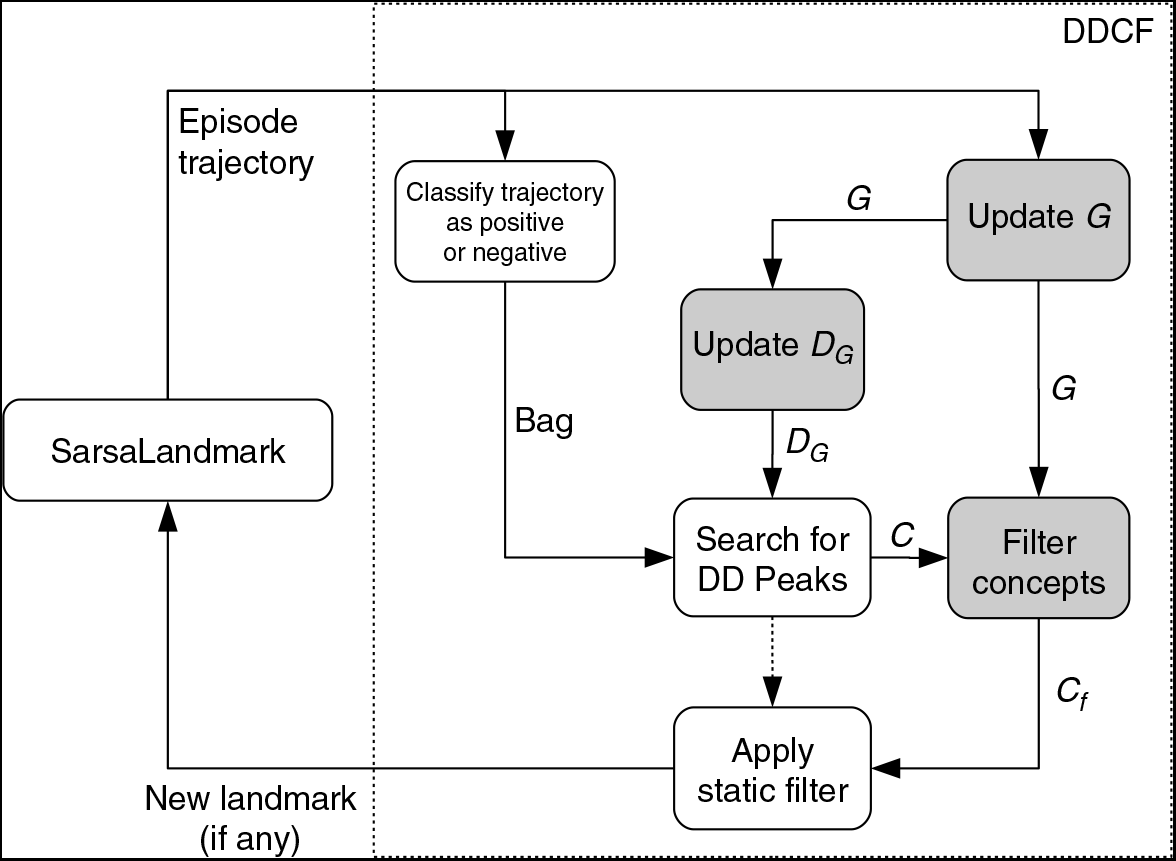
Our proposal synthesizes two approaches, SarsaLandmark and DD, building up a complete framework. The main workflow of the overall framework has the following steps (Figure 1):
initially, SarsaLandmark starts with an empty set of landmarks,
at the end of each episode, the episodic trajectory is fed to DD,
DD classifies the given trajectory as either positive or negative according to a success criteria,
with the given set of bags, the method calculates the DD value for each concept in their concept set,
if a concept is a consistent peak in DD values, that is, it has the highest DD value among the other concepts for several number of episodes, it is marked as a landmark,
then the landmark set of SarsaLandmark is updated and the algorithm uses this set in its update rules.
SarsaLandmark with MDD/DDCF workflow. Shaded parts are the steps that DDCF introduces to MDD

The shaded regions in Figure 1 are extensions of DDCF on McGovern’s DD method (MDD). Although SarsaLandmark can safely be coupled with MDD alone, due to MDD requirements, the designer should also provide the distances between concepts. DDCF not only incrementally calculates these distances, but also applies an effective concept filtering mechanism, completing the framework by making all computations free of designer’s intervention, without sacrificing quality and performance.
4 Experiments
4.1 Problem domains
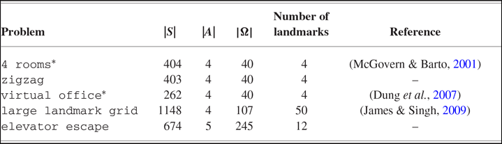
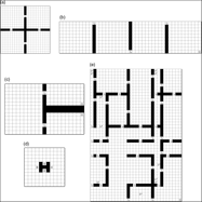
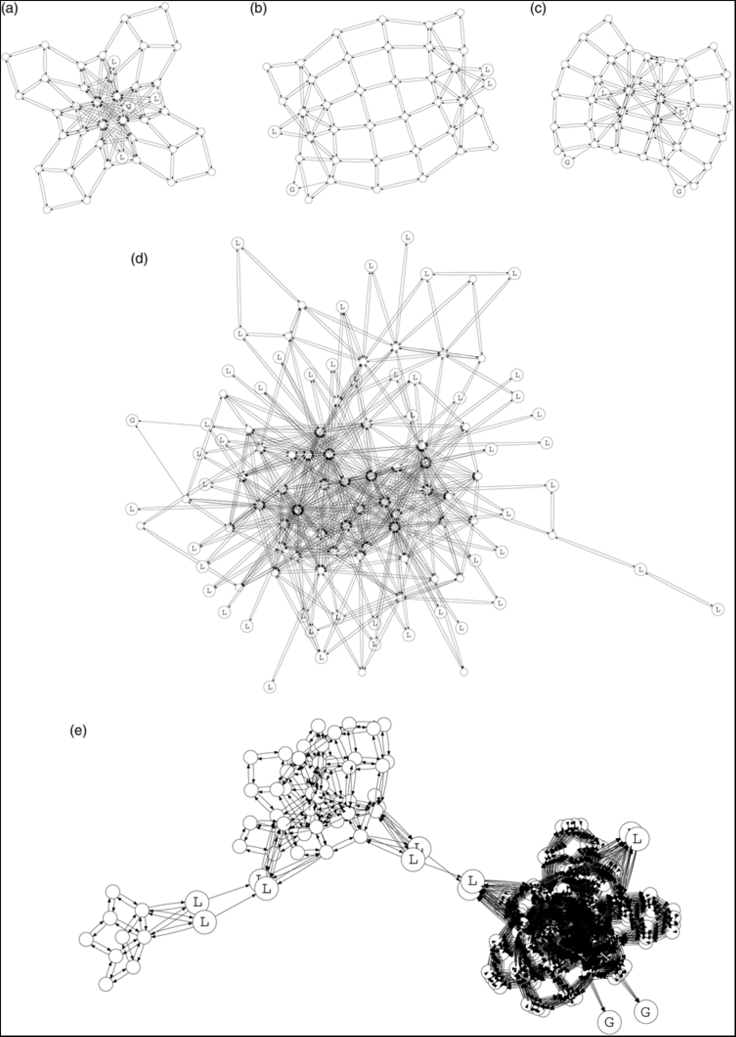
SarsaLandmark with Automatic Landmark Identification using MDD/DDCF is experimented on five problem domains. Three of them (4 rooms, virtual office, and large landmark grid) are known benchmark problems from the literature suitable to experiment for landmarks, while two of them (elevator escape and zigzag) are newly introduced to further analyze special characteristics of the method. 4 rooms and virtual office problems are modified in such a way that they contain landmark states only on the doorways, and large landmark grid is one of the large problems that was introduced in (James & Singh, Reference James and Singh2009). The problem sizes with the number of landmarks (including the goal states) and their corresponding references are given in Table 1. To remind or give an idea of the domain characteristics, the domain illustrations and their observation transition graphs are provided in Figures 2 and 3, respectively.
Problem sizes, the number of landmarks in the problems (including the goal states), and their reference publications. The problems marked with * are modified versions of their originals

Domain sketches. In elevator escape, the light switch, the button, and the elevator positions are marked with S, B, and E, and the goal states and the landmark states are marked with G and L in the other domains. The states marked as L* in large landmark grid are the additional landmark states, emerging due to the observation semantics of the problem. (a) 4 rooms (b) zigzag (c) virtual office (d) elevator escape (e) large landmark grid

Observation transition graphs of the domains. The goal states and landmark states are labeled as G and L, respectively. (a) 4 rooms, (b) zigzag, (c) virtual office, (d) large landmark grid, (e) elevator escape

In the problems with multiple connected rooms (all problems except elevator escape), the doorways are the natural landmark states, yielding unique observations. Moreover, in large landmark grid, there are additional landmark states which were not addressed in the original paper (James & Singh, Reference James and Singh2009). Whenever the agent is at equal distances to the surrounding walls of the room, or if the current observation distinguishes that part of the room from any other rooms in the domain, due to the observation semantics of the environment, the corresponding state is a landmark (see Figure 2(e)).
In 4 rooms, zigzag, and virtual office problems, the agent is initially at a random point in the westernmost room(s), and it can execute four deterministic move actions to four neighboring directions; north, east, south, and west. Arriving at a goal state is rewarded with 1.0 while every other transition is punished by −0.01. The agent receives an observation depending on the distance of it to the surrounding walls in the four compass directions (James & Singh, Reference James and Singh2009): one step from the wall, two steps from the wall, closer to the wall in this direction than the other, further from the wall in this direction than the other.
large landmark grid possesses the same action and observation semantics, but the initial states and the rewarding mechanism are different. As in the experiments of the original paper, initially, the agent is located in any of the landmark states (the ones in the original study, marked with L in Figure 2(e)). Upon reaching the goal state, it gathers a reward of 20, and other movements do not have a reward or a punishment.
elevator escape is a domain that we propose, which contains an inherent partitioning in terms of its observation space, as three subregions separated by landmarks. The goal of the agent is to escape from a  $11\times11$ grid (Figure 2(d)) by using an elevator. In order to call an elevator, it needs to press the button, and in order to see the button, it needs to turn on the lights by the light switch. The locations of the elevators, the button, and the light switch are marked by E, B, and L, respectively. When the agent presses the button, randomly only one of the elevator doors open. Button press and light switch actions are irreversible, that is, the agent cannot turn off the lights once they are on and pressing the button when the elevator door is open has no effect. With this structure, a state in this problem is formed by four features: agent’s position, the light state (on or off), the button state (pressed or not pressed), and the position of the elevator whose door is to open. The agent starts from any position in the grid (except the elevator positions) with the lights off and the button unpressed. The goal state is defined as: the lights are on, the button is pressed, and the agent is in the elevator position with the door open.
The actions are deterministic. In addition to the movement actions north, east, south, and west, the agent can take an interact action for both turning the lights on and pressing the elevator button. Reaching to the goal state is rewarded by 100.0, while the agent gets a −1.0 punishment for any other action.
The observation semantics of the problem is as follows: in the first observational subregion, the lights are off and the agent only possesses a basic vision of observing whether there is a wall in any of the four directions or not. After the lights are turned on, which is the second subregion, the agent acquires an improved vision, allowing it to get an observation according to the distance to the walls in each of the four compass directions (just like in the other grid world domains). Finally, in the third subregion, the pressing of the elevator button opens one of the elevator doors, and the agent starts to hear the music playing in the elevator, in addition to its improved vision. However, the agent’s hearing sensor is noisy. It gives the correct direction of the elevator with probability 0.8 and a random direction with probability 0.2. In addition to this observation semantics, the agent achieves a unique observation when it is in states E, B, and L, which are, by definition, the landmarks of the problem. Consequently, there are 12 landmarks including the goal states. The observation transition graph of the problem is given in Figure 3(e).
Each problem domain has its own characteristics providing a different aspect to show the impact of landmarks on learning performance. 4 rooms problem is, compared to the others, an easy task since the goal state resides in a doorway, leading to an early convergence of a policy. zigzag is of a similar size in terms of state and observation sets; however, an ordered visitation to the landmarks is necessary to reach the goal state. Additionally, the agent should devise a different policy for every room by overcoming the challenge that each room yields almost the same observation semantics. large landmark grid is the largest problem in our problem set, with plenty of landmarks. virtual office contains multiple goal states which is another challenge for the agent. Unlike a bottleneck state in a state transition graph, the observation transition graphs clearly illustrate how a landmark can be located as if it is redundant on the way to goal, which makes its identification much more challenging (Figures 3(a), 3(b), 3(d), and 3(e)). On the other hand, observation transition graph of elevator escape domain has a structure where the observations of the landmark states act as bottlenecks, diving the problem into sub-problems (Figure 3(e)), although this scenario is usually unlikely in real world situations. Note that none of the problems tested here has a memoryless policy solution.
4.2 Experiment settings
Since the contribution here is two-fold, the experiments were designed accordingly. In one aspect, the experimentation needs to show that automatic landmark identification framework (i.e., SarsaLandmark with MDD or DDCF) not only just works but also performs no worse than its manual counterparts (i.e., Sarsa(λ) and SarsaLandmark). On the other hand, we also need to provide empirical evidence that DDCF outperforms McGovern’s original DD heuristic (MDD) for non-Markovian problem settings.
SarsaLandmark with DDCF was tested against SarsaLandmark with MDD, while maintaining Sarsa(λ) and the original SarsaLandmark results as baselines. The results are averaged over 50 experiments where each episode ended with either the agent’s arrival to a goal state or upon reaching 5000 action steps. The experiments for 4 rooms and virtual office were run for 2000 episodes, and experiments for the other domains were run for 10 000 episodes.
For both DD heuristics (i.e., MDD and DDCF), a single observation was considered as a concept. MDD was provided the shortest path distances between the concepts before learning, while DDCF calculated them throughout learning. We employed a step threshold for a bag to be positive so that the methods managed to collect enough number of positive and negative bags. Also, we used  $\theta = 8.8$ and
 $\lambda = 0.9$. In the DD search, we preferred to pick the concepts acting as peak values in the resulting DD distribution, instead of simply selecting the maximum value. In all experiments, both DD versions were executed in the initial 200 episodes.
In order to test the landmark identification performance of both MDD and DDCF, we have compared precision and recall values by using the set of landmarks in the problems as ground truth. Here, precision is defined as the ratio of the number of true landmarks in the identified set to the size of the identified set where recall is defined as the ratio of the number of true landmarks in the identified set to the total number of landmarks in the problem. That is, precision and recall represent accuracy and coverage of the identification, respectively.
For Sarsa(λ),  $\lambda = 0.9$ is used as in (Loch & Singh, Reference Loch and Singh1998). To ensure enough exploration, an
 $\epsilon$-greedy action selection mechanism was used, where the agent takes a random action with probability
 $\epsilon$ and an action according to the current policy with probability
 $(1-\epsilon)$. All of the Sarsa algorithms incorporated
 $\alpha = 0.01$,
 $\gamma = 0.9$, and employed a linear
 $\epsilon$ decay, starting from
 $0.5$ down to 0. While SarsaLandmark extended with MDD and DDCF identified the landmarks online, SarsaLandmark was provided with the landmarks in advance. In large landmark grid, however, only the landmarks marked with L in Figure 2(e) were used, even though there are additional ones in the problem, as described in previous sections.
4.3 Results and discussion
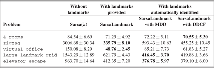
Table 2 shows the average number of steps during learning for each algorithm of discourse. Sarsa(λ) acts as a baseline and it is clear that SarsaLandmark significantly improves learning performance (by a factor ranging from  $1.2$ to
 $8.9$) by means of the additional landmark information. The landmark information which is provided by the designer before learning improves the policy update mechanism and accelerates learning, verifying the effectiveness of SarsaLandmark.
Average number of steps taken in the problem domains. The values are given with their 95% confidence interval

However, when SarsaLandmark is coupled with a DD mechanism, not only the landmarks are identified automatically throughout learning, but also a similar learning performance is achieved compared to SarsaLandmark. This result indicates that DD can effectively be incorporated in identification of landmarks for problems with hidden states, without sacrificing solution quality. Moreover, we can argue that DD is more focused on useful landmarks on the way to a goal state, so that it reaches to the goal states much faster than SarsaLandmark with provided landmarks in the large problems. Overall, in all of the domains, SarsaLandmark with automatic landmark identification outperforms Sarsa(λ), in terms of policy convergence.
Moreover, there is no significant difference between learning performances of SarsaLandmark, SarsaLandmark with MDD, and SarsaLandmark with DDCF. So, we can comfortably conclude that automatic landmark identification framework removes the necessity to identify the landmarks by analyzing the problem beforehand. SarsaLandmark with automatic landmark identification is clearly a forward step to adopt the landmark idea to more realistic problems.
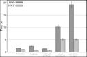
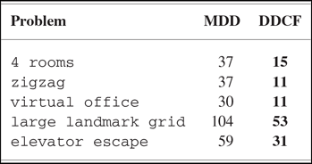
Focusing on automatic landmark identification approaches, it can be clearly seen in Figure 4 that DDCF significantly outperforms MDD in terms of computation time. For all problem domains, DDCF requires much less time to identify landmarks, simply because the size of the DD search concept set is reduced, thanks to the concept filtering heuristic (Table 3). Additionally, as the observation transition graph matures by the early phases of learning, calculation of shortest path distances takes relatively less time compared to the DD calculations of the remaining concepts.
Average CPU time usage for DD approaches

Number of concepts used for automatic landmark identification.

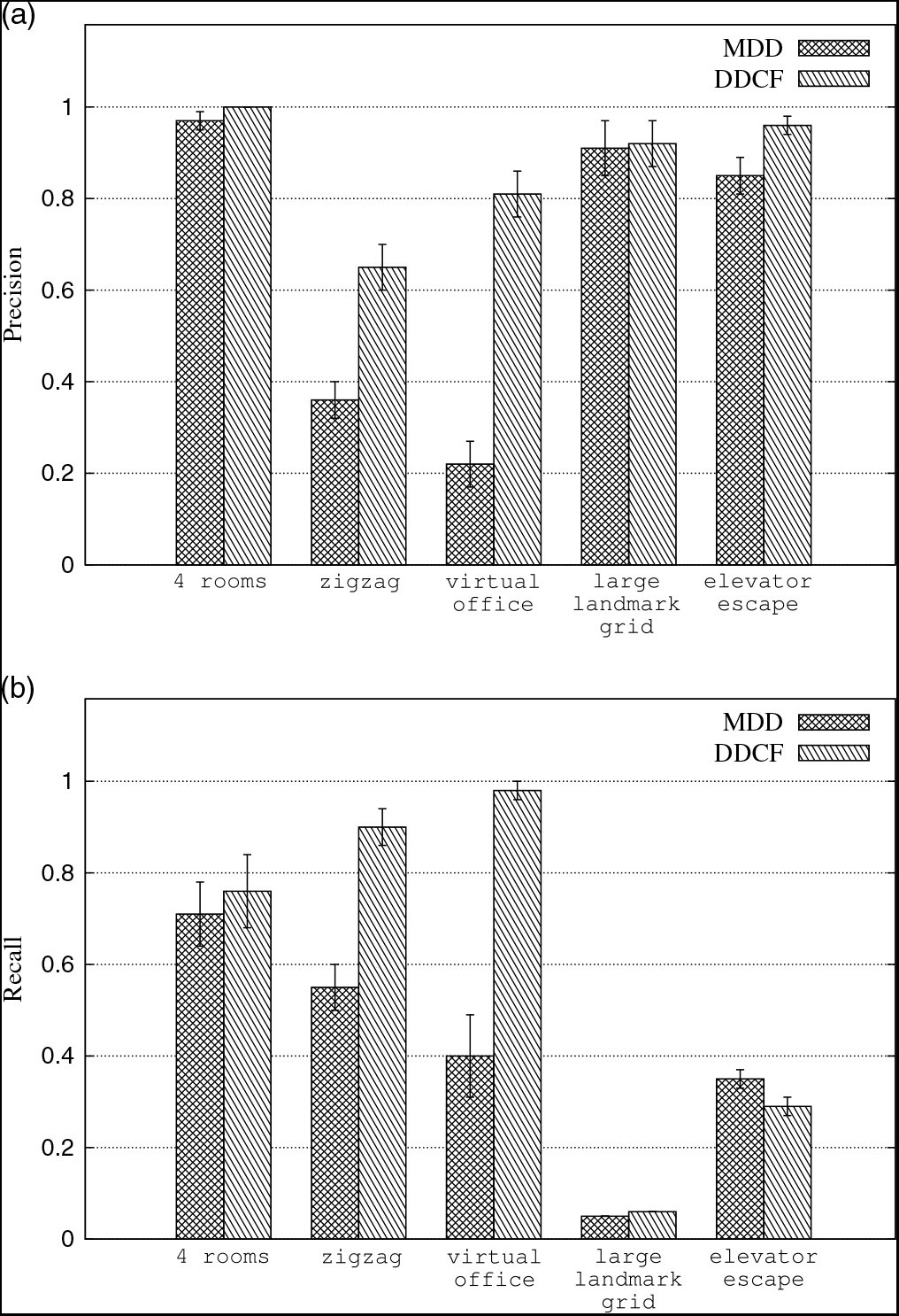
DDCF not only operates faster than MDD, but also seems to produce higher quality solutions. Figure 5(a) shows that DDCF is more precise in finding landmarks for all problem domains, that is, DDCF’s resulting set of identified states contains more of the real landmarks of the problems, compared to MDD. This means that the concept filtering heuristic eliminates some of the concepts that create noise. Moreover, the recall performance of DDCF is also generally higher than MDD, showing a bigger coverage of the true landmark set and meaning that DDCF has a tendency to identify more of the landmarks that the problems contain. The recall value for large landmark grid is low for both of the DD methods. What we observe here is that the agent is more directed to the goal state as the learning proceeds, causing less exploration. In order to identify a bigger set of landmarks, DD requires more data covering these landmarks. Also DD tends to favor the concepts that are seen in the path to a goal state, and some of the landmarks in large landmark grid do not play a key role in such paths. We argue that the performance of DD is dependent on the way the agent traverses the environment, that is, the agent has to visit a landmark frequently in order for DD to identify it.
Precision and recall comparisons of DDCF against MDD (a): Precision, (b): Recall

For zigzag and virtual office domains, for example, the observation transition structure seems to cause static filter of the DD mechanism to fail, since all landmark observations are in the same observational distance to the goal observation, including both the distant landmark states and the landmark states that are close to the goal state (although they are all in different locations in terms of the underlying state transition graph). This is why using a relatively high static filter eliminates useful landmarks, while a low static filter introduces noise to the results. DDCF seems to get rid of this problem via its concept filtering heuristic, since it eliminates those observations yielded by the states closer to the goal state(s).
Another interesting aspect of DDCF worth mentioning is that its identification covers more landmarks than MDD in all of the domains except elevator escape. In elevator escape domain (Figure 3(e)), the local comparison of our concept filtering guides the method to pick the observation of only one of the landmarks in between the observational subregions since only one of them has the observation with the maximum congestion ratio value within its neighborhood.
5 Conclusion
The contribution of this paper is two-fold. As the primary contribution, we propose a RL framework, called SarsaLandmark with Automatic Landmark Identification, for problems with hidden states. The proposed framework enhances its predecessor (James & Singh, Reference James and Singh2009) (which is an adaptation of a well-known on-policy learning algorithm Sarsa(λ) to Landmark-POMDPs), so that it removes the necessity to provide the landmarks of the domain prior to learning, since they are automatically identified during learning. For this purpose, we incorporate DD approach (McGovern & Barto, Reference McGovern and Barto2001), which has been known to effectively identify bottleneck regions in solution space. To our knowledge, this is the first study in RL literature that manages to automatically identify landmarks on-line, and use them in the learning procedure for problems with hidden states.
As a secondary contribution, we elaborate on our short paper (Demir et al., Reference Demir, Çilden and Polat2017) which introduces concept filtering by using a novel graph-based metric, congestion ratio. We not only show DD with Concept Filtering (DDCF) to be applicable in Landmark-POMDPs, but also provide empirical evidence that it significantly improves landmark identification performance and quality, with much less computation effort compared to the original DD method, without any prior information about the problem.
The resulting algorithm SarsaLandmark with Automatic Landmark Discovery removes the necessity for the agent to know in advance when it is in a landmark state. It also possesses a learning performance very close to SarsaLandmark, for which the designer ought to provide all landmarks prior to learning. Experiment results indicate that the combination of SarsaLandmark with DD is a step forward to apply SarsaLandmark to real life problems.
A possible follow-up to this study can focus on improving the DD’s identification performance further and use the presence of landmark states in other policy learning algorithms. Another apparent future work involves making use of temporal ordering of identified landmarks to improve learning performance. Moreover, although the experimentation in this paper focuses on discrete state and action spaces, DDCF can be adapted for continuous spaces with a proper discretization method, which seems to be an immediate extension.
Acknowledgement
The authors would like to thank Hüseyin Aydm for his support.