1 Introduction
Spontaneous reversal phenomena are common in many buoyancy-driven fluid dynamical systems, including reversals of the Earth’s geomagnetic field (Glatzmaier & Roberts Reference Glatzmaier and Roberts1995), and large-scale fluid motion in the sea and the atmosphere (van Doorn et al. Reference van Doorn, Dhruva, Sreenivasan and Cassella2000). There also exist flow reversals of the large-scale circulation (LSC) in a model problem, i.e. Rayleigh–Bénard convection (RBC) where a fluid layer is heated from below and cooled from above (see Ahlers, Grossmann & Lohse Reference Ahlers, Grossmann and Lohse2009; Xia Reference Xia2013; Verma, Kumar & Pandey Reference Verma, Kumar and Pandey2017, and references therein). The study of flow reversals in a model system like RBC may enable us to gain more insights into general reversal phenomena in nature (Huang et al. Reference Huang, Wang, Xi and Xia2015).
In cylindrical cells, there are two categories of flow reversals (Brown, Nikolaenko & Ahlers Reference Brown, Nikolaenko and Ahlers2005): one is rotation-led reversals, which are caused by incessant azimuthal meandering of the circulating plane; the other is cessation-led reversals, in which the LSC slows to a stop and restarts in a random new orientation. Flow reversals in cylindrical cells have been studied both experimentally (Brown et al.
Reference Brown, Nikolaenko and Ahlers2005; Brown & Ahlers Reference Brown and Ahlers2006; Xi, Zhou & Xia Reference Xi, Zhou and Xia2006; Xi & Xia Reference Xi and Xia2007, Reference Xi and Xia2008a
,Reference Xi and Xia
b
; Xi et al.
Reference Xi, Zhang, Hao and Xia2016) and numerically (Mishra et al.
Reference Mishra, De, Verma and Eswaran2011). Several models, either stochastic ones (Benzi Reference Benzi2005; Brown & Ahlers Reference Brown and Ahlers2007) or deterministic ones (Araujo, Grossmann & Lohse Reference Araujo, Grossmann and Lohse2005), have been proposed to account for the flow reversals. The model proposed by Brown & Ahlers (Reference Brown and Ahlers2007) consists of two stochastic ordinary differential equations, and it agrees well with many experimental results for LSC dynamics. The recent experimental work of Xi et al. (Reference Xi, Zhang, Hao and Xia2016) found that the second mode and the remaining higher-order modes play important roles in the dynamical process of the reversal and the Nusselt number
 $Nu$
drops to its minimum during a flow reversal. It was once thought that cessation-led reversals presumably would prevail in systems where the rotational invariance is broken (Brown et al.
Reference Brown, Nikolaenko and Ahlers2005). However, the cessations of the LSC have not been observed in a cubic cell where the rotational invariance is broken (Foroozani et al.
Reference Foroozani, Niemela, Armenio and Sreenivasan2017). It is still ambiguous why cessations are absent in a cubic cell.
Without complicated three-dimensional (3D) structures, flow reversals in two-dimensional (2D) (Sugiyama et al.
Reference Sugiyama, Ni, Stevens, Chan, Zhou, Xi, Sun, Grossmann, Xia and Lohse2010; Chandra & Verma Reference Chandra and Verma2011, Reference Chandra and Verma2013; Petschel et al.
Reference Petschel, Wilczek, Breuer, Friedrich and Hansen2011; Podvin & Sergent Reference Podvin and Sergent2015; Verma, Ambhire & Pandey Reference Verma, Ambhire and Pandey2015; Castillo-Castellanos, Sergent & Rossi Reference Castillo-Castellanos, Sergent and Rossi2016; Xia et al.
Reference Xia, Wan, Liu, Wang and Sun2016; Mannattil et al.
Reference Mannattil, Pandey, Verma and Chakraborty2017; Podvin & Sergent Reference Podvin and Sergent2017) or quasi-2D (Huang et al.
Reference Huang, Wang, Xi and Xia2015; Ni, Huang & Xia Reference Ni, Huang and Xia2015; Huang & Xia Reference Huang and Xia2016) square cavities have attracted much attention in recent years. Sugiyama et al. (Reference Sugiyama, Ni, Stevens, Chan, Zhou, Xi, Sun, Grossmann, Xia and Lohse2010) studied flow reversals in a square cavity with unit aspect ratio by means of 2D direct numerical simulations (DNS) combined with experiments performed in a quasi-2D cell, and found that the results of experiments and simulations are in very good agreement. They also showed that the growth of corner rolls both in kinetic energy and in size plays key roles in triggering flow reversals. They concluded that flow reversals in a 2D/quasi-2D cell occur only in a limited parameter space, that is to say, the reversals do not exist for too large or too small
 $Pr$
as well as too large or too small
 $Ra$
. Chandra & Verma (Reference Chandra and Verma2011, Reference Chandra and Verma2013) used a mode decomposition method to study flow reversals, and showed that flow reversals are caused by a vortex reconnection of two attracting rolls and the appearance of the
 $(2,2)$
mode is critical to trigger flow reversals. Podvin & Sergent (Reference Podvin and Sergent2015, Reference Podvin and Sergent2017) used proper orthogonal decomposition to study flow reversals in a 2D square cell and proposed a 3D model that is based on the interaction of the LSC, the quadrupolar flow and horizontal rolls. Castillo-Castellanos et al. (Reference Castillo-Castellanos, Sergent and Rossi2016) found that the reversal cycle is composed of three successive phases: acceleration, accumulation and release including a rebound event. Huang & Xia (Reference Huang and Xia2016) experimentally found that the frequency of flow reversals increases drastically in smaller
 $\unicode[STIX]{x1D6E4}$
cells. It should be noted that 2D/quasi-2D convection promotes reversals particularly for topological reasons. In 3D cubic cells, reversals are very rare (Foroozani et al.
Reference Foroozani, Niemela, Armenio and Sreenivasan2017). Previous works are almost restricted to a unit-aspect-ratio cell where there exists only one LSC that spans the size of the convection cell. It has already been realized by Sugiyama et al. (Reference Sugiyama, Ni, Stevens, Chan, Zhou, Xi, Sun, Grossmann, Xia and Lohse2010) that
 $\unicode[STIX]{x1D6E4}$
has a strong effect on the reversal dynamics. For a
 $\unicode[STIX]{x1D6E4}=2$
cell, the flow is characterized by two main rolls and flow reversals also exist (Chandra & Verma Reference Chandra and Verma2011; Verma et al.
Reference Verma, Ambhire and Pandey2015). However, much less work has so far been devoted to flow reversals in a
 $\unicode[STIX]{x1D6E4}=2$
cell.
There are several differences between flow reversals in 2D/quasi-2D and 3D geometries. Firstly, the mean time between successive reversals has a strong
 $Ra$
dependence in the former (Sugiyama et al.
Reference Sugiyama, Ni, Stevens, Chan, Zhou, Xi, Sun, Grossmann, Xia and Lohse2010) while it has a weak
 $Ra$
dependence in the latter (Brown & Ahlers Reference Brown and Ahlers2006; Xi & Xia Reference Xi and Xia2007). Secondly, flow reversals in 2D/quasi-2D cells occur in a limited parameter space, and there are no reversals for
 $Ra$
larger than
 $5\times 10^{8}$
(2D) or
 $1.6\times 10^{9}$
(quasi-2D) (Sugiyama et al.
Reference Sugiyama, Ni, Stevens, Chan, Zhou, Xi, Sun, Grossmann, Xia and Lohse2010). However, flow reversals in 3D cylindrical cells can occur at larger
 $Ra~(Ra>10^{10})$
(Brown et al.
Reference Brown, Nikolaenko and Ahlers2005; Brown & Ahlers Reference Brown and Ahlers2006; Xi et al.
Reference Xi, Zhang, Hao and Xia2016) and high
 $Pr~(Pr=19.4)$
(Xie, Wei & Xia Reference Xie, Wei and Xia2013). Whether 2D reversals and cessation-led reversals correspond to the same phenomenon is still an open question (Castillo-Castellanos et al.
Reference Castillo-Castellanos, Sergent and Rossi2016).
Almost all previous studies are conducted in a symmetrical system. However, flow reversals in the real world usually take place in an asymmetrical system. One example is that the heat flux on the core–mantle boundary in the Earth is non-uniform (Gubbins et al.
Reference Gubbins, Sreenivasan, Mound and Rost2011) and this has a great influence on the frequency of geomagnetic reversals (Glatzmaier et al.
Reference Glatzmaier, Coe, Hongre and Roberts1999). Another is the solar convection zone that has both torsional oscillations and periodic reversals (Howard & LaBonte Reference Howard and LaBonte1980). Therefore, it is important to study the influence of symmetry breaking on flow reversals. Brown & Ahlers (Reference Brown and Ahlers2006, Reference Brown and Ahlers2008) found that flow reversals in a
 $\unicode[STIX]{x1D6E4}=1$
cylindrical container are suppressed significantly even for very small tilt angles. Sun, Xi & Xia (Reference Sun, Xi and Xia2005) also found that, in a cylindrical container with
 $\unicode[STIX]{x1D6E4}=0.5$
, a minor tilt of
 $2^{\circ }$
will lock the LSC in the azimuthal plane along the tilted direction, and reversals are suppressed; similar results were also found in a rectangular cell with
 $\unicode[STIX]{x1D6E4}=0.5$
(Wang et al.
Reference Wang, Xu, Xia, Wan and Sun2017). Xia et al. (Reference Xia, Wan, Liu, Wang and Sun2016) studied non-Oberbeck-Boussinesq (NOB) effects on flow reversals, and, interestingly, they found that, when considering NOB effects, flow reversals can be observed for relatively small
 $Pr=0.71$
. Huang et al. (Reference Huang, Wang, Xi and Xia2015) studied the influence of thermal boundary conditions on flow reversals. They claimed that the reversal of the LSC can be viewed as a process for the system to restore its symmetry in a statistical way.
It is generally accepted that tilt will suppress flow reversals in a
 $\unicode[STIX]{x1D6E4}=1$
cell. However, how cell tilt will influence flow reversals in larger-aspect-ratio cells where multiple convection rolls may exist is still an open question. In this paper, we try to fill this gap by studying the influence of cell tilt on flow reversals in a 2D rectangular cell with
 $\unicode[STIX]{x1D6E4}=2$
where two convection rolls may develop; the results are also compared with those for
 $\unicode[STIX]{x1D6E4}=1$
cases. The reason why we choose
 $\unicode[STIX]{x1D6E4}=2$
is that it has been found previously that flow reversals of a double-roll state exist in a
 $\unicode[STIX]{x1D6E4}=2$
cell (Chandra & Verma Reference Chandra and Verma2011; Verma et al.
Reference Verma, Ambhire and Pandey2015), while whether flow reversals exist for
 $\unicode[STIX]{x1D6E4}>2$
is still unknown. There are two advantages of 2D DNS: (i) The numerical effort required for 2D simulations is much smaller and thus we can study flow reversals in a considerable fraction of the Rayleigh number
 $Ra$
/Prandtl number
 $Pr$
versus tilt angle
 $\unicode[STIX]{x1D6FD}$
parameter space for different
 $\unicode[STIX]{x1D6E4}$
. (ii) The flow visualization is much easier, and a detailed flow reversal scenario can be obtained. In recent years, 2D DNS has been used widely to study turbulent convection. For example, it has been used to study turbulent heat transfer (van der Poel, Stevens & Lohse Reference van der Poel, Stevens and Lohse2011; van der Poel et al.
Reference van der Poel, Stevens, Sugiyama and Lohse2012, Reference van der Poel, Ostilla-Mónico, Verzicco and Lohse2014; Huang & Zhou Reference Huang and Zhou2013; Bao et al.
Reference Bao, Chen, Liu, She, Zhang and Zhou2015), to study boundary layer (BL) dynamics (Zhou et al.
Reference Zhou, Stevens, Sugiyama, Grossmann, Lohse and Xia2010, Reference Zhou, Sugiyama, Stevens, Grossmann, Lohse and Xia2011; van der Poel et al.
Reference van der Poel, Ostilla-Mónico, Verzicco, Grossmann and Lohse2015; Zhang et al.
Reference Zhang, Huang, Jiang, Liu, Lu, Qiu and Zhou2017a
), to reveal NOB effects on flow organization (Sugiyama et al.
Reference Sugiyama, Calzavarini, Grossmann and Lohse2009), to probe the effect of roughness on heat transfer (Shishkina & Wagner Reference Shishkina and Wagner2011; Toppaladoddi, Succi & Wettlaufer Reference Toppaladoddi, Succi and Wettlaufer2017; Zhu et al.
Reference Zhu, Stevens, Verzicco and Lohse2017; Xu et al.
Reference Xu, Wang, Wan, Yan and Sun2018; Zhang et al.
Reference Zhang, Sun, Bao and Zhou2018), to investigate statistics of kinetic and thermal energy dissipation rates in RBC (Zhang, Zhou & Sun Reference Zhang, Zhou and Sun2017b
) and, more recently, to explore the transition to the ultimate regime (Zhu et al.
Reference Zhu, Mathai, Stevens, Verzicco and Lohse2018).
The remainder of the paper is organized as follows. In § 2, we introduce the governing equations and numerical methods. The main results are presented in § 3, which is divided into three parts. Section 3.1 studies the influence of tilt on flow reversals in
 $\unicode[STIX]{x1D6E4}=1$
and
 $\unicode[STIX]{x1D6E4}=2$
cells. In § 3.2, we use a mode decomposition method to reveal the inherent mechanism for the reversals in a tilted
 $\unicode[STIX]{x1D6E4}=2$
cell. Section 3.3 discusses the heat transfer properties during the reversals. Finally, a short summary is presented in § 4.
2 Numerical procedures
We studied flow reversals in a tilted cell with width
 ${\hat{W}}$
and height
 ${\hat{H}}$
(hatted quantities are dimensional), where the bottom plate has a constant high temperature
 $\hat{T}_{H}$
while the top plate has a constant low temperature
 $\hat{T}_{C}$
. Here, with Oberbeck–Boussinesq approximation, the dimensionless governing equations read
 $$\begin{eqnarray}\displaystyle & \displaystyle \unicode[STIX]{x1D735}\boldsymbol{\cdot }\boldsymbol{u}=0, & \displaystyle\end{eqnarray}$$
 $$\begin{eqnarray}\displaystyle & \displaystyle \frac{\unicode[STIX]{x2202}\boldsymbol{u}}{\unicode[STIX]{x2202}t}+\boldsymbol{u}\boldsymbol{\cdot }\unicode[STIX]{x1D735}\boldsymbol{u}=-\unicode[STIX]{x1D735}p+\sqrt{\frac{Pr}{Ra}}\unicode[STIX]{x1D6FB}^{2}\boldsymbol{u}+T\boldsymbol{e}, & \displaystyle\end{eqnarray}$$
 $$\begin{eqnarray}\displaystyle & \displaystyle \frac{\unicode[STIX]{x2202}T}{\unicode[STIX]{x2202}t}+\boldsymbol{u}\boldsymbol{\cdot }\unicode[STIX]{x1D735}T=\frac{1}{\sqrt{Ra\,Pr}}\unicode[STIX]{x1D6FB}^{2}T, & \displaystyle\end{eqnarray}$$
where
 $\boldsymbol{u}=(v,w)$
and
 $\boldsymbol{x}=(y,z)$
are the velocity components and coordinates in the horizontal and vertical directions,
 $p$
is the reduced kinetic pressure,
 $T$
is the temperature,
 $\boldsymbol{e}$
is a unit vector defined by
 $\boldsymbol{e}=(\sin (\unicode[STIX]{x1D6FD}),\cos (\unicode[STIX]{x1D6FD}))$
, and
 $\unicode[STIX]{x1D6FD}$
is the tilt angle, which is positive when the cell rotates anticlockwise. For non-dimensionalization, the free-fall velocity
 $\hat{U} =({\hat{g}}\hat{\unicode[STIX]{x1D6FC}}\unicode[STIX]{x0394}\hat{T}{\hat{H}})^{1/2}$
and the height of the container
 ${\hat{H}}$
are used, where
 ${\hat{g}}$
is the gravitational acceleration,
 $\hat{\unicode[STIX]{x1D6FC}}$
is the isobaric thermal expansion coefficient, and
 $\unicode[STIX]{x0394}\hat{T}=\hat{T}_{H}-\hat{T}_{C}$
is the temperature difference. The reference time is the free-fall time
 $\hat{t}_{f}={\hat{H}}/\hat{U}$
, and the dimensionless temperature is defined by
 $T=(\hat{T}-\hat{T}_{C})/\unicode[STIX]{x0394}\hat{T}$
. This problem is governed by three dimensionless parameters, i.e. the Prandtl number
 $Pr$
, Rayleigh number
 $Ra$
and aspect ratio
 $\unicode[STIX]{x1D6E4}$
:
 $$\begin{eqnarray}Pr=\frac{\hat{\unicode[STIX]{x1D708}}}{\hat{\unicode[STIX]{x1D705}}},\quad Ra=\frac{{\hat{g}}\hat{\unicode[STIX]{x1D6FC}}\unicode[STIX]{x0394}\hat{T}{\hat{H}}^{3}}{\hat{\unicode[STIX]{x1D708}}\hat{\unicode[STIX]{x1D705}}},\quad \unicode[STIX]{x1D6E4}=\frac{{\hat{W}}}{{\hat{H}}},\end{eqnarray}$$
where
 $\hat{\unicode[STIX]{x1D705}}$
is the thermal diffusivity, and
 $\hat{\unicode[STIX]{x1D708}}$
is the kinematic viscosity. No-slip and impermeability conditions are imposed at all walls and the sidewalls are insulated.
The governing equations are solved numerically by a well-validated in-house code lMn2d. All spatial terms are discretized using a second-order central difference scheme. A non-uniform grid with clustered grid points near walls is used to resolve small scales inside boundary layers. Pressure and velocities are staggered in space in order to avoid pressure–velocity decoupling. Time integration is accomplished by using the Adams–Bashforth scheme for the nonlinear terms and the Crank–Nicolson scheme for the viscous and diffusion terms. Detailed numerical schemes and validations of this code can be found in our previous work (Xia et al. Reference Xia, Wan, Liu, Wang and Sun2016).
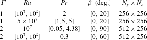
The simulation parameters of this paper are listed in table 1. The initial field for cases with
 $\unicode[STIX]{x1D6FD}=0^{\circ }$
is the conductive state with small perturbations added to the temperature field, while for tilted cases we use the flow field of
 $\unicode[STIX]{x1D6FD}=0^{\circ }$
as the initial condition. In all cases, the simulations run for a long time to determine whether flow reversals exist. Moreover, in order to obtain better statistics of the flow reversal frequencies, the longest simulation is performed for 249 000 free-fall time units.
Simulation parameters. The columns from left to right indicate aspect ratio, Rayleigh number, Prandtl number, tilt angle and mesh resolution.

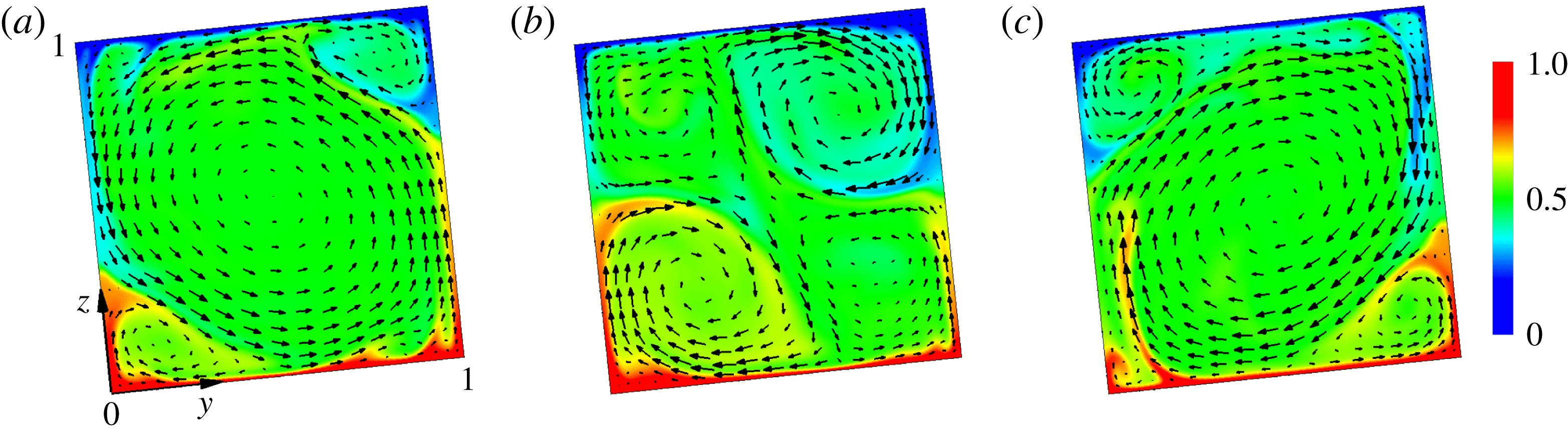
Three snapshots of the temperature field superimposed with velocity vectors during one of the flow reversals for
 $Ra=5\times 10^{7},~Pr=2,~\unicode[STIX]{x1D6FD}=6^{\circ }$
at different times: (a)
 $t=500$
, (b)
 $t=655$
and (c)
 $t=705$
.

3 Results and discussion
3.1 Flow reversals in two-dimensional tilted cells
We start by studying the influence of tilt on flow reversals for a typical aspect ratio
 $\unicode[STIX]{x1D6E4}=1$
. Figure 1 shows snapshots of the temperature and velocity fields during one of the reversals at
 $Ra=5\times 10^{7}$
,
 $Pr=2$
and
 $\unicode[STIX]{x1D6FD}=6^{\circ }$
. Although the symmetry of the system is broken, it is found that the reversal process is similar to the level case (Sugiyama et al.
Reference Sugiyama, Ni, Stevens, Chan, Zhou, Xi, Sun, Grossmann, Xia and Lohse2010). The two corner rolls grow simultaneously in kinetic energy and also in size due to the plume detachment from the boundary layers, until they merge as a new LSC with the opposite direction, and a flow reversal happens. It is well known that flow reversals occur in a certain
 $Ra{-}Pr$
parameter space for
 $\unicode[STIX]{x1D6E4}=1$
. For a system with only one main roll, the reversal process can be nicely indicated by a global quantity, i.e. the net angular momentum
 $$\begin{eqnarray}L(t)=\langle -(z-1/2)v(\boldsymbol{x},t)+(y-1/2)w(\boldsymbol{x},t)\rangle _{V},\end{eqnarray}$$
where
 $\langle \cdot \rangle _{V}$
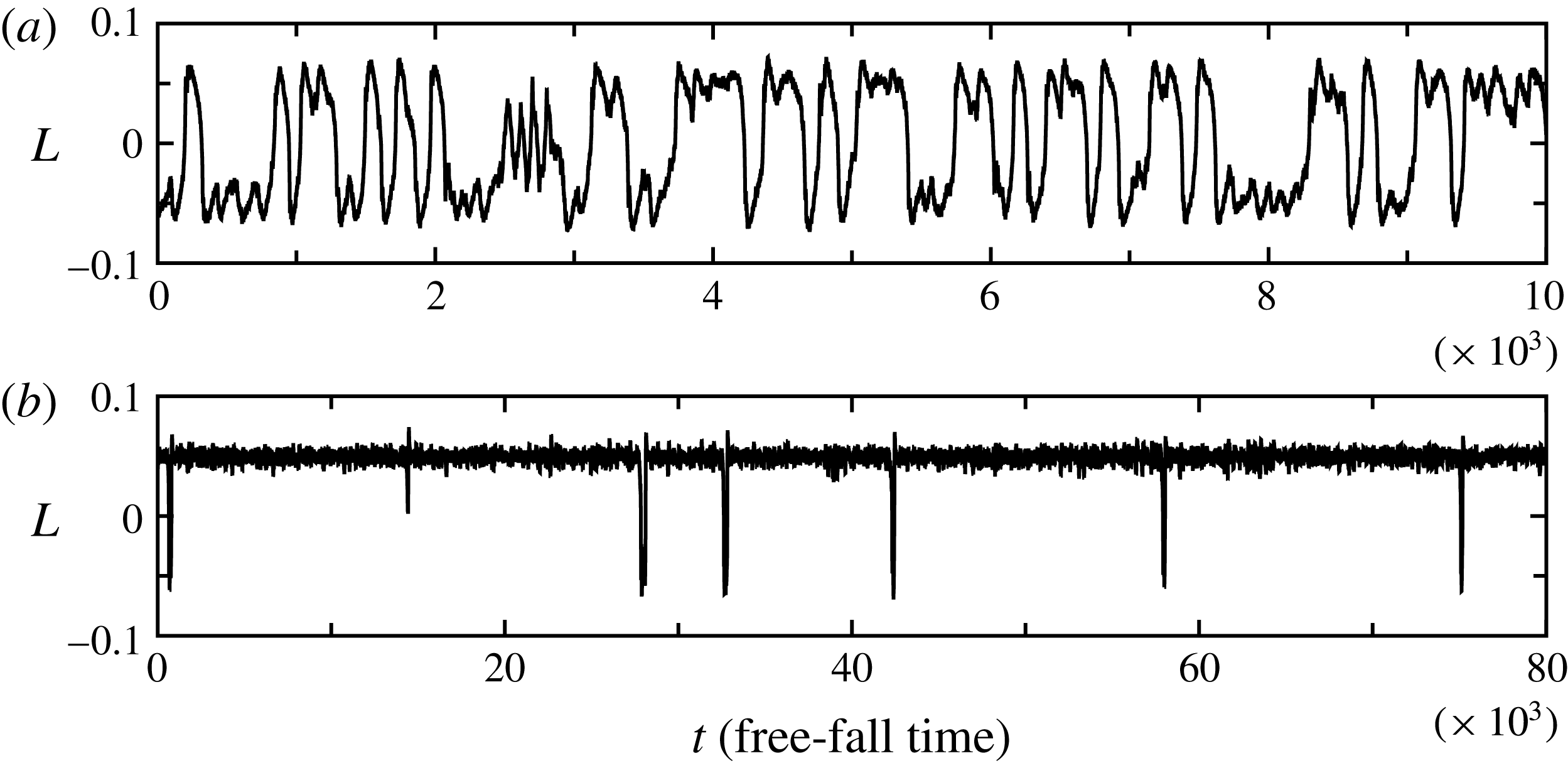
represents averaging over the total area. Figure 2 shows the time evolution of
 $L$
for the level case with
 $\unicode[STIX]{x1D6FD}=0^{\circ }$
and the tilted case with
 $\unicode[STIX]{x1D6FD}=6^{\circ }$
at
 $Ra=5\times 10^{7}$
and
 $Pr=2$
. A sign change of
 $L$
can reveal a reversal; frequent flow reversals in a level cell can be observed in figure 2(a). From figure 2(b), it is evident that the symmetry breaking induced by tilt greatly suppresses flow reversals for
 $\unicode[STIX]{x1D6E4}=1$
. One sees that the clockwise main roll with negative
 $L$
stays for quite a short time before reversing its orientation. This is because, for the clockwise LSC, as shown in figure 1(c), tilt introduces a horizontal buoyancy force along the
 $y$
direction so that the hot plumes are more likely to move up to the bottom-right corner roll and the cold plumes tend to move down to the top-left corner roll. The two corner rolls have more opportunities to grow and trigger a reversal. Besides, the tilt may weaken the clockwise LSC since along the hot and cold plates the horizontal buoyancy force is in the opposite direction to the flow velocity of LSC. Thus the clockwise LSC is less stable and is easier to reverse its orientation, and it always stays for a much shorter time as shown in figure 2(b). Previous studies have shown that the main roll will be locked in the plane along the tilted direction both in cylindrical cells (Xi, Lam & Xia Reference Xi, Lam and Xia2004; Brown & Ahlers Reference Brown and Ahlers2006; Shishkina & Horn Reference Shishkina and Horn2016) and in rectangular cells (Guo et al.
Reference Guo, Zhou, Cen, Qu, Lu, Sun and Shang2015, Reference Guo, Zhou, Qu, Lu, Sun and Shang2017) with
 $\unicode[STIX]{x1D6E4}=1$
. Thus the suppression of flow reversals by tilt for
 $\unicode[STIX]{x1D6E4}=1$
is within expectation.
Time evolution of the angular momentum
 $L$
for
 $\unicode[STIX]{x1D6E4}=1,~Ra=5\times 10^{7}$
and
 $Pr=2$
: (a)
 $\unicode[STIX]{x1D6FD}=0^{\circ }$
and (b)
 $\unicode[STIX]{x1D6FD}=6^{\circ }$
. The positive and negative signs indicate anticlockwise and clockwise circulations, respectively.

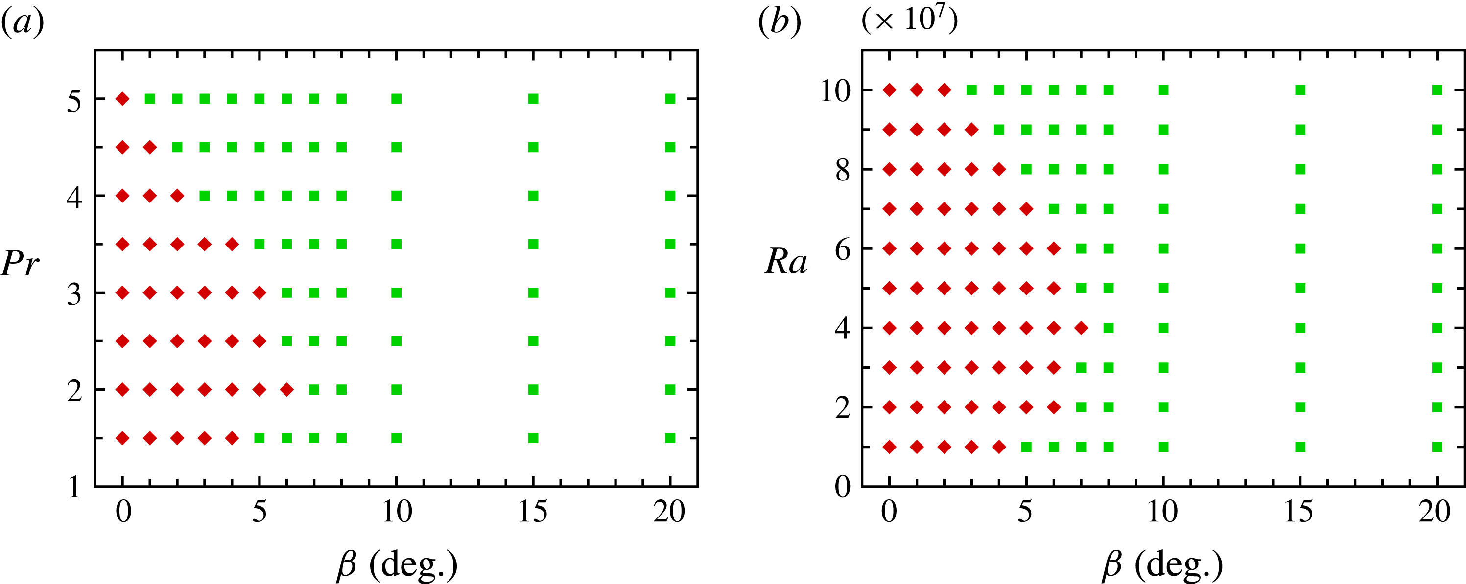
We then map out phase diagrams for
 $\unicode[STIX]{x1D6E4}=1$
over
 $\unicode[STIX]{x1D6FD}{-}Pr$
parameter space with
 $Ra=5\times 10^{7}$
and over
 $\unicode[STIX]{x1D6FD}{-}Ra$
parameter space with
 $Pr=2$
in figure 3. We run for at least 5000 large-eddy turnover times
 $t_{E}$
to detect whether flow reversals exist. Time
 $t_{E}$
is defined by
 $t_{E}:=4\unicode[STIX]{x03C0}/\langle |\unicode[STIX]{x1D714}_{c}(t)|\rangle$
, where
 $\unicode[STIX]{x1D714}_{c}$
denotes vorticity in the centre of the main roll. For some cases (for example,
 $Ra=10^{8},~Pr=2,~\unicode[STIX]{x1D6E4}=1,~\unicode[STIX]{x1D6FD}=3^{\circ }$
), we even calculate for more than
 $10\,000\,t_{E}$
to conclude there are indeed no reversals. As shown in figure 3(a), the critical angle
 $\unicode[STIX]{x1D6FD}_{c}$
displays a non-monotonic relation with
 $Pr$
. For larger
 $Pr$
, the
 $\unicode[STIX]{x1D6FD}_{c}$
value is smaller; for
 $Pr=5$
, a minor tilt of
 $1^{\circ }$
will completely suppress flow reversals due to the fact that the thickness of the thermal BL is much smaller than the thickness of the kinetic BL and thermal coupling between the corner roll and the thermal BL is weakened, as stated previously (Sugiyama et al.
Reference Sugiyama, Ni, Stevens, Chan, Zhou, Xi, Sun, Grossmann, Xia and Lohse2010). For small
 $Pr$
, thermal diffusion becomes dominant and suppresses the growth of the corner roll. Therefore, flow reversals in the tilted cell also occur more easily at intermediate
 $Pr$
, and the corresponding
 $\unicode[STIX]{x1D6FD}_{c}$
is also larger. In figure 3(b),
 $\unicode[STIX]{x1D6FD}_{c}$
also displays a non-monotonic relation with
 $Ra$
. For intermediate
 $Ra$
, the corresponding
 $\unicode[STIX]{x1D6FD}_{c}$
is larger. The reason lies in the non-monotonic dependence of the flow reversal frequency on
 $Ra$
. It can be seen in figure 3 of Sugiyama et al. (Reference Sugiyama, Ni, Stevens, Chan, Zhou, Xi, Sun, Grossmann, Xia and Lohse2010) that flow reversals are most frequent for intermediate
 $Ra$
(approximately
 $7\times 10^{7}$
for
 $Pr=4.3$
); any increase or decrease of
 $Ra$
will reduce the flow reversal frequency. For the
 $Pr=2$
considered in our work, the reversals are most frequent for
 $Ra\sim 4\times 10^{7}$
, thus the corresponding
 $\unicode[STIX]{x1D6FD}_{c}$
is larger, and any increase or decrease of
 $Ra$
will reduce
 $\unicode[STIX]{x1D6FD}_{c}$
. The reversals occur less and less frequently with increasing
 $Ra$
and reversals disappear when
 $Ra\geqslant 2\times 10^{8}$
for
 $Pr=2$
(Sugiyama et al.
Reference Sugiyama, Ni, Stevens, Chan, Zhou, Xi, Sun, Grossmann, Xia and Lohse2010). Thus the main roll here is more sensitive to tilt at larger
 $Ra$
, and a minor tilt of the cell will suppress flow reversals at relatively high
 $Ra$
.
(a) Phase diagram in the
 $\unicode[STIX]{x1D6FD}{-}Pr$
plane for
 $Ra=5\times 10^{7},~\unicode[STIX]{x1D6E4}=1$
. (b) Phase diagram in the
 $\unicode[STIX]{x1D6FD}{-}Ra$
plane for
 $Pr=2,~\unicode[STIX]{x1D6E4}=1$
. Red filled diamonds (♦) correspond to detected flow reversals, and green squares (▪) to a single-roll state without reversals.

Compared with
 $\unicode[STIX]{x1D6E4}=1$
, there have been fewer studies devoted to horizontally adjacent double-roll reversals in a
 $\unicode[STIX]{x1D6E4}=2$
cell (Chandra & Verma Reference Chandra and Verma2011; Verma et al.
Reference Verma, Ambhire and Pandey2015). Here, we first explore the flow reversals in a
 $\unicode[STIX]{x1D6E4}=2$
cell at a fixed
 $Ra=10^{7}$
, but varying
 $Pr$
and
 $\unicode[STIX]{x1D6FD}$
, as listed in table 1. The
 $Ra$
dependence for a fixed
 $Pr=0.3$
is also studied. Figure 4 shows flow reversal scenarios for a level case with
 $Ra=10^{7}$
,
 $Pr=0.71$
and
 $\unicode[STIX]{x1D6E4}=2$
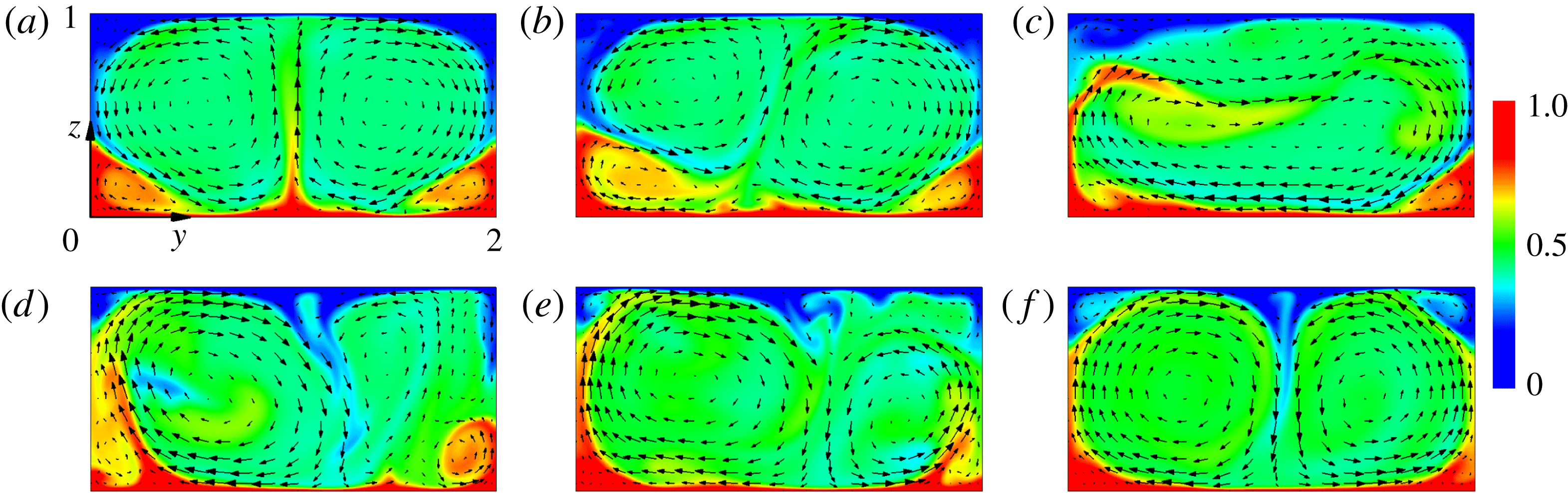
; it is seen that the single corner roll growth leads to a flow reversal, which is qualitatively the same as that of Verma et al. (Reference Verma, Ambhire and Pandey2015). Owing to the inherent symmetry of the system, the two bottom corner rolls in figure 4(a) and the two top corner rolls in figure 4(f) all have opportunities to grow and trigger flow reversals. However, when the symmetry of the system is broken by tilt, the two corner rolls will no longer play equivalent roles.
Six snapshots of the temperature field superimposed with velocity vectors during one of the flow reversals for
 $Ra=10^{7},~Pr=0.71,~\unicode[STIX]{x1D6FD}=0^{\circ }$
at different times: (a)
 $t=12\,283$
, (b)
 $t=12\,338$
, (c)
 $t=12\,349$
, (d)
 $t=12\,354$
, (e)
 $t=12\,361$
and (f)
 $t=12\,377$
.

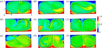
Nine snapshots of the temperature field superimposed with velocity vectors during two of the flow reversals for
 $Ra=10^{7},~Pr=0.71,~\unicode[STIX]{x1D6FD}=1^{\circ }$
at different times: (a)
 $t=1684.5$
, (b)
 $t=1701$
, (c)
 $t=1704$
, (d)
 $t=1710$
, (e)
 $t=1711.5$
, (f)
 $t=1725$
, (g)
 $t=2860.5$
, (h)
 $t=2869.5$
and (i)
 $t=2890.5$
.

Figure 5 shows snapshots for two successive flow reversals at
 $Ra=10^{7},~Pr=0.71$
and
 $\unicode[STIX]{x1D6FD}=1^{\circ }$
. As shown in figure 5(a), the flow field is characterized by two main rolls and two bottom corner rolls. Since tilt will introduce a horizontal buoyancy force along the
 $y$
direction, the hot plumes detached from the lower BL will bear a top-right buoyancy force and be apt to feed the bottom-right corner roll. This is favourable for the growth of the bottom-right corner roll as illustrated in figure 5(b). The bottom-left corner roll, however, almost remains unchanged. The subsequent reversal process shown in figure 5(c–f) is similar to that in a level case. Similarly, for the next reversal cycle, due to the
 $y$
direction buoyancy force introduced by tilting the cell, the cold plumes detached from the upper BL are more likely to enter the top-left corner roll. Thus the top-left corner roll growth will lead to a flow reversal, as shown in figure 5(g–i). It should also be noted that the horizontal buoyancy force induced by tilt near the top and bottom walls is always in the opposite direction to the flow velocity of one of the two main rolls. Thus the effect of tilt on the main rolls may always play some roles in flow reversals in a tilted
 $\unicode[STIX]{x1D6E4}=2$
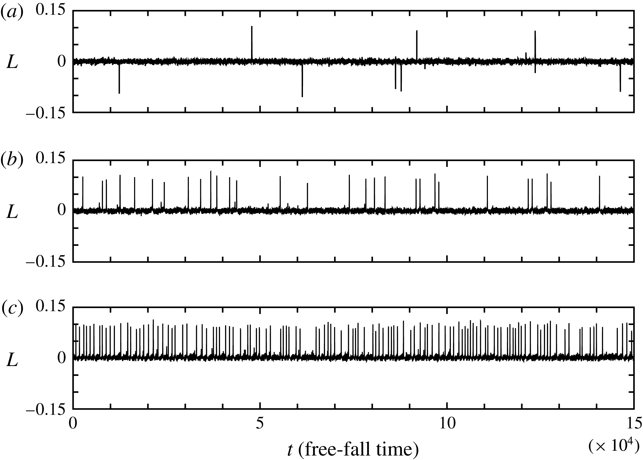
cell, and the unstable clockwise main roll will always first reverse its direction. Owing to the symmetry breaking, only the bottom-right corner roll in figure 5(a) and the top-left corner roll in figure 5(f) have opportunities to grow and lead to a flow reversal; this is different from a level case where the four corner rolls all have opportunities to grow and trigger a flow reversal. This argument can be quantitatively demonstrated by investigating the long-time evolution of
 $L$
as shown in figure 6. Note that
 $L$
is calculated with respect to the centre point
 $(1,0.5)$
here. The flow is dominated by the double-roll mode with
 $L\simeq 0$
most of the time due to compensation of two main rolls. When flow reversal occurs, the clockwise/anticlockwise intermediate single-roll mode appears (see figures 4
c and 5
c), and thus large negative/positive
 $L$
will appear, indicated by sharp spikes in figure 6. The large positive
 $L$
indicates that it is the growth of the bottom-right corner roll shown in figure 5(a) or the top-left corner roll shown in figure 5(f) that leads to flow reversals, while the large negative
 $L$
indicates that it is the growth of the bottom-left corner roll shown in figure 4(a) or the top-right corner roll shown in figure 4(f) that leads to a successful flow reversal. It is seen that both positive and negative spikes exist for the level case while only positive spikes exist for the tilted case. Thus only the growth of the bottom-right corner roll or the top-left corner roll will lead to a flow reversal in a tilted cell. From figure 6, we can also see that there are many more flow reversals in tilted cells, demonstrating that tilt will promote flow reversals for
 $\unicode[STIX]{x1D6E4}=2$
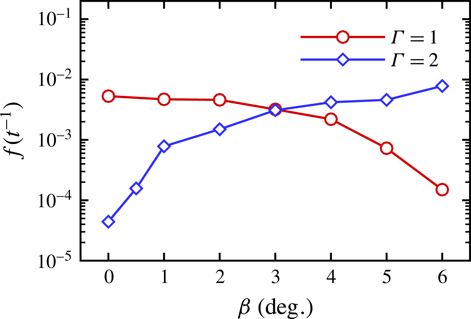
. To further quantify the promoting effect of cell tilt on the flow reversal, the reversal frequencies
 $f$
defined by reversal numbers per free-fall time unit are calculated, which are plotted in figure 7. Clearly, for
 $\unicode[STIX]{x1D6E4}=1$
,
 $f$
does not drop much for small
 $\unicode[STIX]{x1D6FD}\leqslant 2^{\circ }$
, while for
 $\unicode[STIX]{x1D6FD}>2^{\circ }$
,
 $f$
drops rapidly. In contrast,
 $f$
increases monotonically with
 $\unicode[STIX]{x1D6FD}$
for
 $\unicode[STIX]{x1D6E4}=2$
; it even increases more than an order from
 $\unicode[STIX]{x1D6FD}=0^{\circ }$
to
 $1^{\circ }$
. Thus a minor tilt will greatly promote flow reversals for
 $\unicode[STIX]{x1D6E4}=2$
.
Time evolution of angular momentum
 $L$
for
 $Ra=10^{7},~Pr=0.71$
and
 $\unicode[STIX]{x1D6E4}=2$
: (a)
 $\unicode[STIX]{x1D6FD}=0^{\circ }$
, (b)
 $\unicode[STIX]{x1D6FD}=0.5^{\circ }$
and (c)
 $\unicode[STIX]{x1D6FD}=1^{\circ }$
.

Flow reversal frequency
 $f$
as a function of
 $\unicode[STIX]{x1D6FD}$
. Red circles (○) for
 $Ra=5\times 10^{7},~Pr=2,~\unicode[STIX]{x1D6E4}=1$
; blue diamonds (♢) for
 $Ra=10^{7},~Pr=0.71,~\unicode[STIX]{x1D6E4}=2$
.

(a) Phase diagram in the
 $\unicode[STIX]{x1D6FD}{-}Pr$
plane for
 $Ra=10^{7},~\unicode[STIX]{x1D6E4}=2$
. (b) Phase diagram in the
 $\unicode[STIX]{x1D6FD}{-}Ra$
plane for
 $Pr=0.3,~\unicode[STIX]{x1D6E4}=2$
. Red filled diamonds (♦) correspond to detected flow reversals; blue filled circles (●) denote double-roll state without flow reversals; green squares (▪) represent single-roll state without flow reversals.

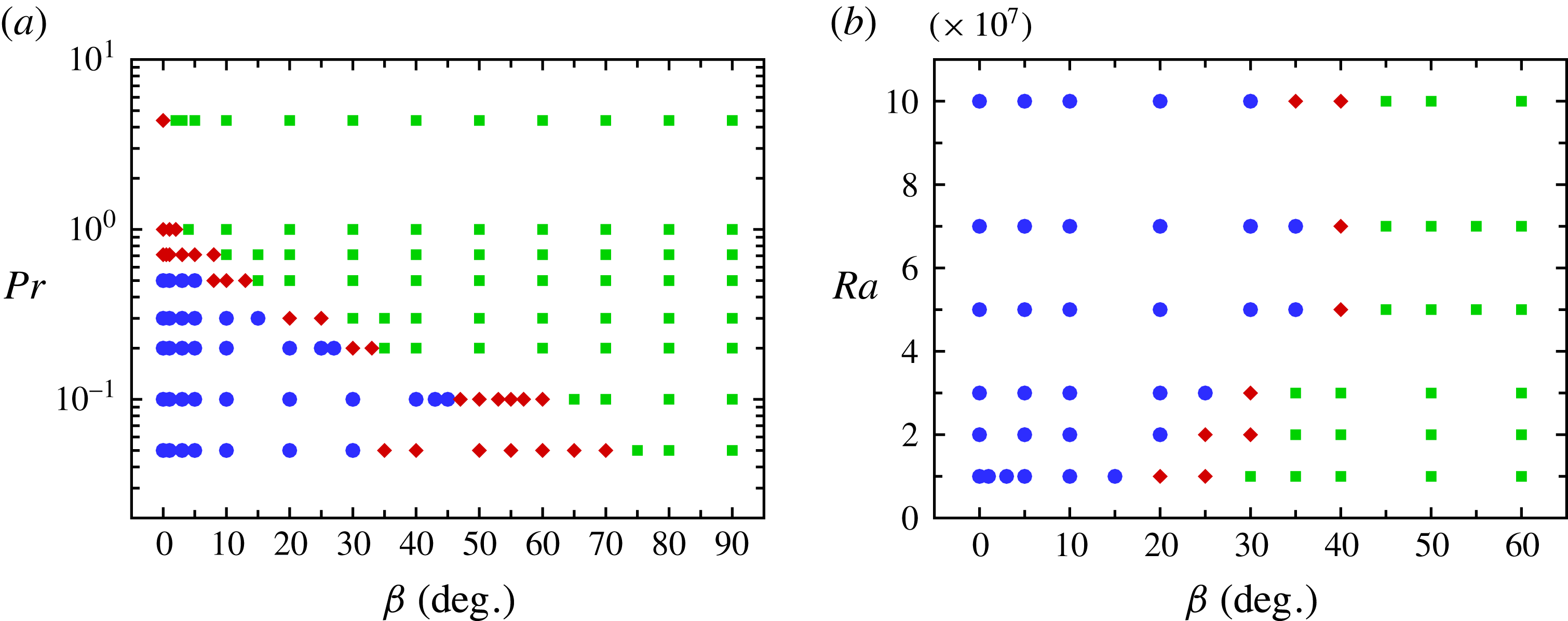
Again we map out flow states in
 $\unicode[STIX]{x1D6FD}{-}Pr$
space for
 $Ra=10^{7}$
and
 $\unicode[STIX]{x1D6E4}=2$
in figure 8(a). We run for at least
 $4000\,t_{E}$
to detect whether flow reversals exist. As the position of the centre of the main roll changes after reversals (this is especially evident for reversals with large
 $\unicode[STIX]{x1D6FD}$
), the large-eddy turnover time
 $t_{E}$
is better defined by
 $t_{E}:=(W+2H)/u_{LSC}$
, where
 $u_{LSC}$
is the typical velocity of the LSC measured at
 ${\sim}H/10$
from the sidewalls and plates (Zhou et al.
Reference Zhou, Sugiyama, Stevens, Grossmann, Lohse and Xia2011; Ni et al.
Reference Ni, Huang and Xia2015). Three different flow states are identified, which are the double-roll state without flow reversals, the double-roll state with flow reversals, and the single-roll state without flow reversals, respectively. One sees that, for
 $Pr\leqslant 0.5$
and small
 $\unicode[STIX]{x1D6FD}$
, the flow stays in the stable double-roll state without flow reversals. When
 $\unicode[STIX]{x1D6FD}$
is beyond a critical value, the double-roll state is no longer stable and flow reversals occur in the intermediate range of
 $\unicode[STIX]{x1D6FD}$
. However, when
 $\unicode[STIX]{x1D6FD}$
increases further, the flow becomes a stable one-roll state and no reversals can be observed any more. For
 $0.71\leqslant Pr\leqslant 4.38$
, the flow transits directly from reversal state to one-roll state. It is interesting that for relatively small
 $Pr\leqslant 0.5$
, flow reversals can only occur in tilted cells. It is worth mentioning that the reversals even occur at very small
 $Pr$
and large
 $\unicode[STIX]{x1D6FD}$
. For instance, there exist flow reversals for
 $Pr=0.05$
and
 $\unicode[STIX]{x1D6FD}=70^{\circ }$
, as seen in figure 8(a). This is in stark contrast to that in a
 $\unicode[STIX]{x1D6E4}=1$
cell where no reversals exist for
 $Pr\leqslant 0.71$
(Sugiyama et al.
Reference Sugiyama, Ni, Stevens, Chan, Zhou, Xi, Sun, Grossmann, Xia and Lohse2010). Because flow reversals in tilted cells with
 $\unicode[STIX]{x1D6E4}=2$
tend to occur for small
 $Pr$
, the
 $Ra$
dependence of flow reversals is studied for a representative small
 $Pr=0.3$
. Figure 8(b) maps out flow states over the
 $\unicode[STIX]{x1D6FD}{-}Ra$
parameter space for fixed
 $Pr=0.3$
. It is obvious that flow reversals can only be found in tilted cells, which even exist at
 $Ra=10^{8}$
. Based on the above findings, we show that the symmetry breaking of the system induced by tilt has considerably broadened the original
 $Ra{-}Pr$
parameter space of flow reversals for
 $\unicode[STIX]{x1D6E4}=2$
. However, the crucial question left in this section is why reversals only occur in a limited range of
 $\unicode[STIX]{x1D6FD}$
for
 $\unicode[STIX]{x1D6E4}=2$
.
3.2 Mode decomposition analysis
To find the answer to the question left in § 3.1, a mode decomposition method is employed. We project the velocity components
 $v$
and
 $w$
onto the following Fourier basis:
 $$\begin{eqnarray}\displaystyle & \displaystyle \hat{v}^{m,n}=\sqrt{2}\sin (m\unicode[STIX]{x03C0}y/2)\cos (n\unicode[STIX]{x03C0}z), & \displaystyle\end{eqnarray}$$
 $$\begin{eqnarray}\displaystyle & \displaystyle {\hat{w}}^{m,n}=-\sqrt{2}\cos (m\unicode[STIX]{x03C0}y/2)\sin (n\unicode[STIX]{x03C0}z). & \displaystyle\end{eqnarray}$$
The velocity can be recovered by
 $$\begin{eqnarray}\displaystyle & \displaystyle v(y,z,t)=\mathop{\sum }_{m,n}A_{y}^{m,n}(t)\hat{v}^{m,n}, & \displaystyle\end{eqnarray}$$
 $$\begin{eqnarray}\displaystyle & \displaystyle w(y,z,t)=\mathop{\sum }_{m,n}A_{z}^{m,n}(t){\hat{w}}^{m,n}. & \displaystyle\end{eqnarray}$$
The projection is done componentwise by a scalar product in the
 $L_{2}$
-space. The corresponding time series
 $A_{y}^{m,n}(t)$
and
 $A_{z}^{m,n}(t)$
can be obtained by
 $$\begin{eqnarray}\displaystyle & \displaystyle A_{y}^{m,n}(t)=\int _{0}^{y_{max}}\int _{0}^{z_{max}}v(y,z,t)\hat{v}^{m,n}\,\text{d}y\,\text{d}z, & \displaystyle\end{eqnarray}$$
 $$\begin{eqnarray}\displaystyle & \displaystyle A_{z}^{m,n}(t)=\int _{0}^{y_{max}}\int _{0}^{z_{max}}w(y,z,t){\hat{w}}^{m,n}\,\text{d}y\,\text{d}z. & \displaystyle\end{eqnarray}$$
A value
 $M^{m,n}(t)$
representing the contribution of different modes can be evaluated by
 $M^{m,n}(t)=\sqrt{A_{y}^{m,n}(t)^{2}+A_{z}^{m,n}(t)^{2}}$
. The mode
 $(m,n)$
corresponds to a flow structure with
 $m$
rolls in the
 $y$
direction and
 $n$
rolls in the
 $z$
direction. Although Fourier basis functions do not satisfy the no-slip boundary conditions, it has been shown that they capture the convective flow profiles well (Chandra & Verma Reference Chandra and Verma2011, Reference Chandra and Verma2013; Petschel et al.
Reference Petschel, Wilczek, Breuer, Friedrich and Hansen2011; Verma et al.
Reference Verma, Ambhire and Pandey2015). The Fourier mode decomposition method has been employed extensively to study 2D reversals (Chandra & Verma Reference Chandra and Verma2011, Reference Chandra and Verma2013; Petschel et al.
Reference Petschel, Wilczek, Breuer, Friedrich and Hansen2011; Verma et al.
Reference Verma, Ambhire and Pandey2015) and heat transfer in quasi-2D cells (Wagner & Shishkina Reference Wagner and Shishkina2013; Chong et al.
Reference Chong, Wagner, Kaczorowski, Shishkina and Xia2018).
We quantitatively analyse the flow mode competition for a representative case with
 $Ra=10^{7},~Pr=0.5$
and
 $\unicode[STIX]{x1D6E4}=2$
where flow reversals only happen in a limited
 $\unicode[STIX]{x1D6FD}$
range, i.e.
 $7^{\circ }\leqslant \unicode[STIX]{x1D6FD}\leqslant 13^{\circ }$
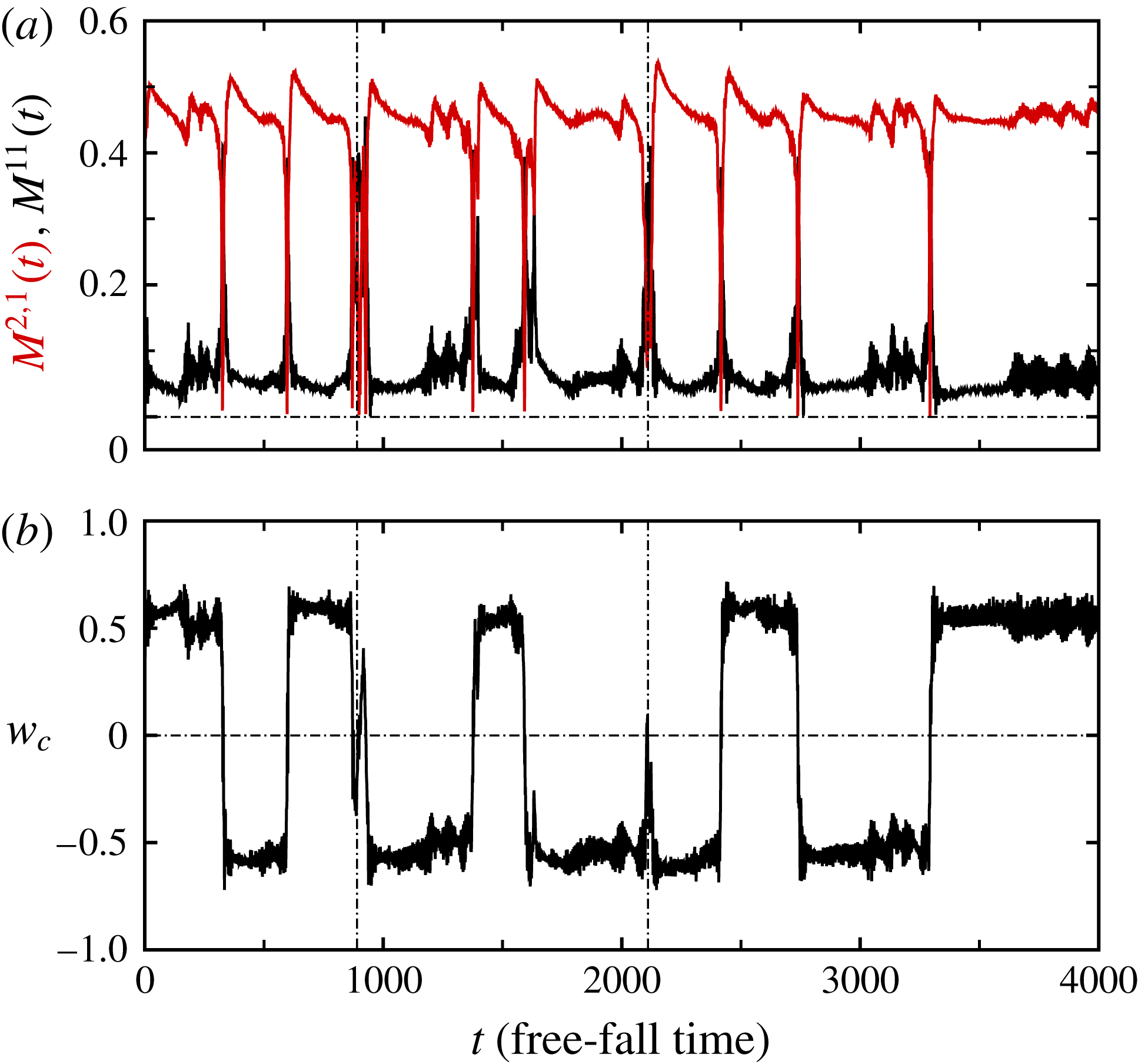
. Figure 9 shows the time evolution of the amplitudes of dominated modes
 $(2,1)$
and
 $(1,1)$
, and the vertical velocity at the centre of the cell
 $w_{c}$
for
 $\unicode[STIX]{x1D6FD}=8^{\circ }$
. A sign change of
 $w_{c}$
can nicely indicate a reversal. The flow near the times
 $t=890$
and
 $2110$
, which are denoted by vertical dash-dotted lines, can be viewed as cessations in a
 $\unicode[STIX]{x1D6E4}=2$
cell. The growth of corner rolls does not trigger successful reversals near these two moments. In figure 9, it is found that the transient
 $M^{2,1}(t)$
approaches zero during reversals, while
 $M^{1,1}(t)$
shows a spike. The vanishing of the
 $(2,1)$
mode and the appearance of the
 $(1,1)$
mode correspond to the appearance of the anticlockwise single-roll structures during the reversal. So we conclude that the appearance of single-roll mode
 $(1,1)$
plays a critical role in triggering a reversal, similar to that in a
 $\unicode[STIX]{x1D6E4}=1$
cell where the
 $(2,2)$
mode plays the dominant role.
For
 $Ra=10^{7},~Pr=0.5$
and
 $\unicode[STIX]{x1D6FD}=8^{\circ }$
, the time evolution of (a) flow mode amplitude of
 $M^{2,1}(t)$
(red line) and
 $M^{1,1}(t)$
(black line); and (b) vertical velocity component
 $w_{c}$
at the centre location
 $(1,0.5)$
.

To understand why the flow reversals occur in a limited range of
 $\unicode[STIX]{x1D6FD}$
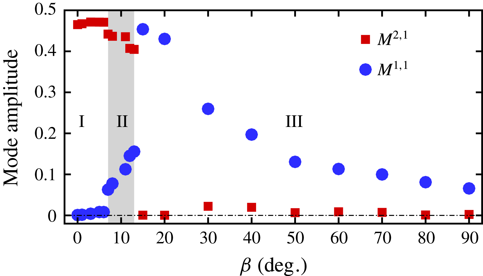
, the bifurcation diagram is further shown in figure 10. One sees that the flow is dominated by the
 $(2,1)$
mode for
 $0^{\circ }\leqslant \unicode[STIX]{x1D6FD}\leqslant 6^{\circ }$
and the amplitude of the
 $(1,1)$
mode approaches 0, which is referred to as regime I. The
 $M^{1,1}$
starts to grow rapidly beyond
 $\unicode[STIX]{x1D6FD}=7^{\circ }$
, then flow reversals occur for
 $7^{\circ }\leqslant \unicode[STIX]{x1D6FD}\leqslant 13^{\circ }$
, and we call this regime II. In this regime, the flow is still dominated by the
 $(2,1)$
mode, but the
 $M^{2,1}$
and
 $M^{1,1}$
are comparable. For
 $15^{\circ }\leqslant \unicode[STIX]{x1D6FD}\leqslant 90^{\circ }$
, the flow is dominated by the
 $(1,1)$
mode and the amplitude of the
 $(2,1)$
mode is close to 0, which is called regime III. It can be seen that the
 $M^{1,1}$
decreases monotonically with increasing
 $\unicode[STIX]{x1D6FD}$
in this regime; this is because the flow strength, which is denoted by the Reynolds number
 $Re$
, decreases monotonically with increasing
 $\unicode[STIX]{x1D6FD}$
in this regime (Guo et al.
Reference Guo, Zhou, Cen, Qu, Lu, Sun and Shang2015; Shishkina & Horn Reference Shishkina and Horn2016). It is clear that the reversals tend to happen in the intermediate
 $\unicode[STIX]{x1D6FD}$
range where the
 $(2,1)$
mode and
 $(1,1)$
mode have comparable strengths. Based on the mode decomposition analysis, we conclude that the flow reversals in tilted cells for
 $\unicode[STIX]{x1D6E4}=2$
can be viewed as a mode competition process between the
 $(2,1)$
mode and
 $(1,1)$
mode.
Time-averaged flow mode amplitudes
 $M^{1,1}$
and
 $M^{2,1}$
as a function of
 $\unicode[STIX]{x1D6FD}$
for
 $Ra=10^{7},~Pr=0.5$
and
 $\unicode[STIX]{x1D6E4}=2$
; the grey area denotes the angle at which flow reversals appear.

3.3 Heat transfer during flow reversals
Finally, we discuss the heat transfer properties during a flow reversal. It is well recognized that heat transfer is closely connected to the mean flow structures in both two dimensions (van der Poel et al.
Reference van der Poel, Stevens and Lohse2011) and three dimensions (Sun et al.
Reference Sun, Xi and Xia2005; Xi & Xia Reference Xi and Xia2008b
; Bailon-Cuba, Emran & Schumacher Reference Bailon-Cuba, Emran and Schumacher2010; Weiss & Ahlers Reference Weiss and Ahlers2011; Xia Reference Xia2011; Huang et al.
Reference Huang, Kaczorowski, Ni and Xia2013; Chong et al.
Reference Chong, Huang, Kaczorowski and Xia2015). As shown above, during a flow reversal, the flow structures change greatly, so a significant change of heat transfer is expected. The Nusselt number (
 $Nu$
), used to measure heat transport, is defined as
 $$\begin{eqnarray}\displaystyle Nu(t)=\frac{\hat{Q}}{\hat{k}\unicode[STIX]{x0394}\hat{T}/{\hat{H}}}=\frac{(\langle \hat{\unicode[STIX]{x1D70C}}{\hat{c}}_{p}{\hat{w}}\hat{T}\rangle _{A}+\langle \hat{k}\unicode[STIX]{x2202}_{z}\hat{T}\rangle _{A})}{\hat{k}\unicode[STIX]{x0394}\hat{T}/{\hat{H}}}, & & \displaystyle\end{eqnarray}$$
where
 $\hat{Q}$
is the heat flux across any horizontal plane (3D) or line (2D), and
 $\langle \cdot \rangle$
denotes averaging over any horizontal plane (3D) or line (2D). Here,
 $Nu$
averaged over the hot and cold plate are denoted as
 $Nu_{h}$
and
 $Nu_{c}$
, respectively.
Time evolution of (a) vertical velocity at the cell centre
 $w_{c}$
, (b) Nusselt number at the hot wall
 $Nu_{h}$
, and (c) Nusselt number at the cold wall
 $Nu_{c}$
, for
 $Ra=10^{7},~Pr=0.71$
and
 $\unicode[STIX]{x1D6FD}=1^{\circ }$
.

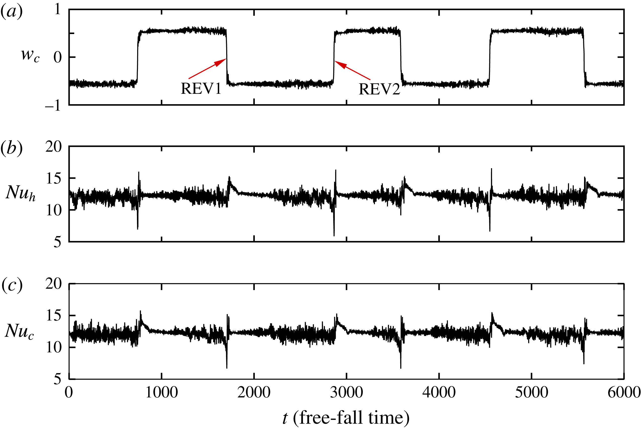
Figure 11 shows the time evolution of the vertical velocity component at the cell centre
 $w_{c}$
,
 $Nu_{h}$
and
 $Nu_{c}$
for
 $Ra=10^{7},~Pr=0.71,~\unicode[STIX]{x1D6E4}=2$
and
 $\unicode[STIX]{x1D6FD}=1^{\circ }$
. We distinguish the two kinds of reversals by the sign change of
 $w_{c}$
, referred to as REV1 and REV2. For REV1,
 $Nu_{h}$
experiences a minor decrease, and then an overshoot; after a relatively long time, it returns to its normal value;
 $Nu_{c}$
has a drastic decrease during the reversal; after an overshoot, it returns to its normal value quickly. For REV2, the behaviour of
 $Nu_{h}$
is similar to that of
 $Nu_{c}$
in REV1 and
 $Nu_{c}$
is similar to that of
 $Nu_{h}$
in REV1. These phenomena are similar to that in a level case. The most significant feature for
 $\unicode[STIX]{x1D6E4}=2$
is that
 $Nu_{h}$
and
 $Nu_{c}$
behave differently during a reversal.
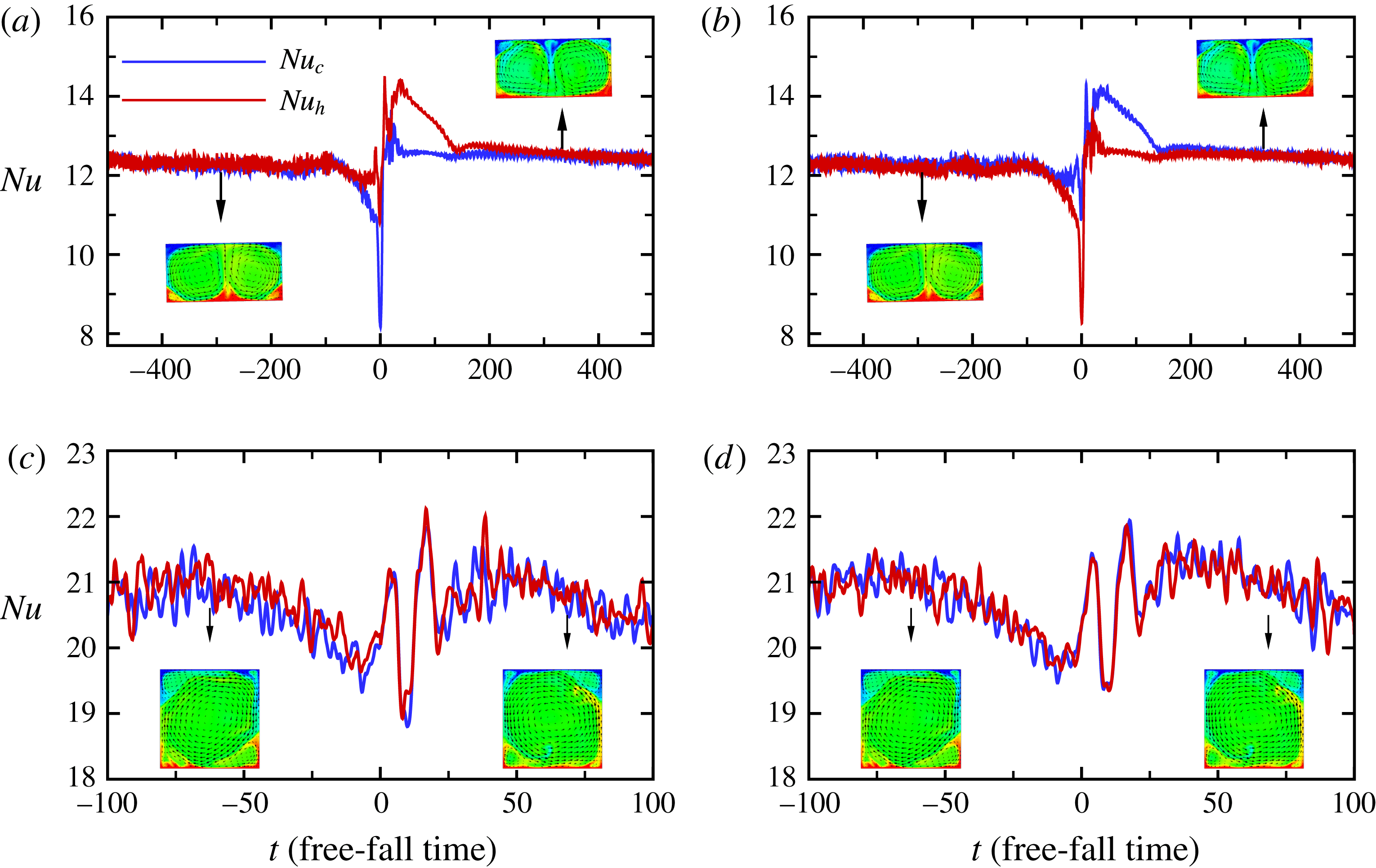
Time evolution of ensemble-averaged
 $Nu_{c}$
and
 $Nu_{h}$
during flow reversals for (a,b)
 $Ra=10^{7}$
,
 $Pr=0.71$
,
 $\unicode[STIX]{x1D6FD}=1^{\circ }$
and
 $\unicode[STIX]{x1D6E4}=2$
and (c,d)
 $Ra=5\times 10^{7}$
,
 $Pr=2$
,
 $\unicode[STIX]{x1D6FD}=0^{\circ }$
and
 $\unicode[STIX]{x1D6E4}=1$
. (a) REV1. (b) REV2. (c) The reversal from the clockwise single-roll mode to the anticlockwise single-roll mode. (d) The inverse process of (c).

To better illustrate this point, the time evolutions of ensemble-averaged
 $Nu_{h}$
and
 $Nu_{c}$
are shown in figure 12. For
 $\unicode[STIX]{x1D6E4}=2$
, we first locate the data point where
 $w_{c}$
becomes zero corresponding to the appearance of a single-roll mode during reversals. Then starting from this data point we go forward and backward for 500 free-fall time units. We averaged over 59/62 samples for REV1/REV2, and the results are plotted in figure 12(a) and (b). Similar procedures were also used before (Castillo-Castellanos et al.
Reference Castillo-Castellanos, Sergent and Rossi2016; Xi et al.
Reference Xi, Zhang, Hao and Xia2016) and in the study of statistical properties of geomagnetic field reversals (Valet et al.
Reference Valet, Fournier, Courtillot and Herrero-Bervera2012). One can see from figure 12(a) that both
 $Nu_{h}$
and
 $Nu_{c}$
drop to their minima at
 $t\approx 0$
corresponding to the appearance of a single-roll mode during REV1. The
 $Nu_{c}$
has a more drastic decrease than
 $Nu_{h}$
, due to apparent top-down asymmetric flow structures as shown in figure 5(c). There is also a small overshoot for
 $Nu_{h}$
before reaching its local minimum. After reaching their local minima, both
 $Nu_{h}$
and
 $Nu_{c}$
increase rapidly. The
 $Nu_{c}$
experiences some fluctuations around its local maximum, and then returns to its normal value. While for
 $Nu_{h}$
, two local maxima are found, and it takes more time for
 $Nu_{h}$
to return to its normal value. For REV2, the behaviours of
 $Nu_{h}$
and
 $Nu_{c}$
are reversed compared to REV1, as shown in figure 12(b). For comparison,
 $Nu_{h}$
and
 $Nu_{c}$
for
 $\unicode[STIX]{x1D6E4}=1$
during two kinds of flow reversals are also plotted in figures 12(c) and 12(d). The time
 $t=0$
is the time when the global angular momentum
 $L$
becomes 0, corresponding to the appearance of the
 $(2,2)$
mode during the reversal, which is top-down symmetric. It is clear that
 $Nu_{h}$
and
 $Nu_{c}$
always have the same trend. It is interesting that the overshoot phenomenon is observed, which is similar to that in a cylindrical cell (Xi et al.
Reference Xi, Zhang, Hao and Xia2016). In short, the heat transfer is directly connected with flow structures. The different trends of
 $Nu_{h}$
and
 $Nu_{c}$
during a reversal in a
 $\unicode[STIX]{x1D6E4}=2$
cell are due to the preference for single corner roll growth during a reversal; while for
 $\unicode[STIX]{x1D6E4}=1$
, two corner rolls grow simultaneously, and the flow structure is symmetrical about the horizontal centreline, thus
 $Nu_{c}$
and
 $Nu_{h}$
behave the same.
4 Summary
In this work, we investigate the effect of cell tilt on flow reversals in
 $\unicode[STIX]{x1D6E4}=1$
and
 $2$
cells by performing 2D DNS. It is found that flow reversals are suppressed by tilt for
 $\unicode[STIX]{x1D6E4}=1$
. However, flow reversals characterized by two main rolls are greatly promoted by tilt for
 $\unicode[STIX]{x1D6E4}=2$
. For
 $\unicode[STIX]{x1D6E4}=1$
, flow reversals in tilted cells are led by the simultaneous growth of two corner rolls, which is qualitatively the same as those in level cases. For
 $\unicode[STIX]{x1D6E4}=2$
, due to the introduction of a horizontal buoyancy force by tilt, flow reversals in a tilted cell are always led by the growth of the bottom-right or the top-left corner roll, which is different from those in a level case, where the four corner rolls all have opportunities to grow and trigger a reversal. Tilt is favourable for the thermal plumes to feed the bottom-right or the top-left corner roll, thus breaking the balance between the two main rolls and leading to a reversal. As a result, the reversals are promoted by tilt and are much more frequent than those in level cells. Moreover, flow reversals in tilted cells with
 $\unicode[STIX]{x1D6E4}=2$
tend to occur for small
 $Pr$
. Tilt broadens the
 $Ra$
–
 $Pr$
parameter space for flow reversals to happen in a
 $\unicode[STIX]{x1D6E4}=2$
cell. Our study expands the flow reversals in a canonical system to small
 $Pr$
, which is relevant to many geophysical and astrophysical flows (Schumacher, Götzfried & Scheel Reference Schumacher, Götzfried and Scheel2015; Scheel & Schumacher Reference Scheel and Schumacher2016). By exploiting the large-scale mode decomposition analysis, we demonstrate that flow reversals in a tilted cell with
 $\unicode[STIX]{x1D6E4}=2$
can be viewed as a mode competition process between the single-roll mode and horizontally adjacent double-roll mode. Reversals can only occur in an intermediate range of
 $\unicode[STIX]{x1D6FD}$
where
 $M^{1,1}$
and
 $M^{2,1}$
are comparable. Furthermore, we find that
 $Nu_{h}$
and
 $Nu_{c}$
behave the same during a reversal for
 $\unicode[STIX]{x1D6E4}=1$
, but they behave differently for
 $\unicode[STIX]{x1D6E4}=2$
due to preference for single corner roll growth during a reversal.
The present finding of more frequent flow reversals in a tilted
 $\unicode[STIX]{x1D6E4}=2$
cell demonstrates that the effects of symmetry breaking on flow reversals are system-dependent, which should still be explored in asymmetrical systems to gain more physical insights into the various reversal phenomena in nature.
Acknowledgements
This work is supported by the National Natural Science Foundation of China under grants 11572314, 11502137, 11772323 and 11621202, and by the Fundamental Research Funds for the Central Universities.