




No CrossRef data available.
BIAS REDUCTION IN NONPARAMETRIC DIFFUSION COEFFICIENT ESTIMATION
Published online by Cambridge University Press: 04 August 2003
Abstract
In this paper, we quantify the asymptotic bias of the Florens-Zmirou (1993, Journal of Applied Probability 30, 790–804) and Jiang and Knight (1997, Econometric Theory 13, 615–645) estimator for the diffusion coefficient when the step of discretization is fixed, and then we propose a bias adjustment that partially compensates for the distortion. Also, we show that our estimators have all the asymptotic properties of the Florens-Zmirou and Jiang and Knight estimator when the step of discretization goes to zero. We provide some examples.I thank the editor Peter C.B. Phillips and the two referees for comments and suggestions that led to considerable improvement of the paper. I am also grateful to Carlos Braumann and Tom Kundert for helpful comments. This research was supported by the Fundação para a Ciência e a Tecnologia (FCT) and by POCTI.
Information
- Type
- Research Article
- Information
- Copyright
- © 2003 Cambridge University Press
1. INTRODUCTION
Stochastic continuous-time processes, especially diffusion processes, have been widely used in physical and biological sciences and, more recently, in financial economics. In mathematical finance the success of the diffusion continuous-time approach can be attributed to its many attractive properties (see Merton, 1990).
However, all models involve unknown parameters or functions, which need to be estimated from observations of the process. The estimation of diffusion processes is therefore a crucial step in all applications, in particular, in applied finance. Nonparametric estimation based on continuous sampling observations has been considered in the literature for many years (see references in Rao, 1999). However, as has been stressed by various authors, the continuous sampling observations hypothesis is unreasonable because, in practice, it is obviously impossible to observe a process continuously over any given interval, as a result, for instance, of the limitations on the precision of the measuring instrument or of the unavailability of observations at every point in time (Rao, 1999). It is therefore natural that the most recent research in diffusion processes estimation has been concerned with discrete time observations, where some progress has been made, in both parametric and nonparametric estimation. In nonparametric estimation based on discrete-time observations Florens-Zmirou (1993) proposes an estimator for the diffusion coefficient using a uniform kernel, without imposing any restrictions on the drift coefficient. Aït-Sahalia (1996) proposes a semiparametric estimation procedure for the diffusion term based on a parametric drift coefficient. Stanton (1997) builds approximations to the infinitesimal coefficients. Jiang and Knight (1997) use the Florens-Zmirou estimator with a Gaussian kernel for the diffusion coefficient and propose a drift estimator based on the diffusion coefficient estimator and the stationary (or marginal) density. Hansen, Scheinkman, and Touzi (1998) propose spectral methods to recover the infinitesimal coefficients from the stationary density and an eigenvalue-eigenfunction pair of the conditional expectation operator. More recently, Bandi and Phillips (2003) have developed an asymptotic theory for nonparametric estimates of the drift and diffusion coefficients, under broad assumptions on the data generating process. In particular, they do not require the existence of a time-invariant marginal data density, and thus stationarity is not needed.
We consider the stochastic differential equation (1) subsequently with unknown coefficients a and b. The X process is observed at instants {ti = Δn, i = 0,1,…,n}, where Δn is the step of discretization. To estimate the diffusion coefficient b2(x) consistently it is well known that, in principle, it is not necessary that the time span tn go to infinity (see Bandi and Phillips, 2003). Nevertheless, a crucial but to some extent unrealistic assumption, in both cases of estimation (drift and diffusion coefficients), is that Δn → 0 as n increases. In fact, in most empirical applications the step of discretization is generally fixed, i.e., Δn = Δ as n increases. For example, the series could be daily, weekly, or monthly.
In this paper, we quantify the asymptotic bias of the Florens-Zmirou (1993) and Jiang and Knight (1997) estimator for the diffusion coefficient when the step of discretization is fixed (as tn = nΔ → +∞), and then we propose a bias adjustment that partially compensates for the distortion. This is done by including the drift coefficient or its nonparametric estimates in the diffusion estimator, which, as we will see, enables a reduction of the asymptotic bias. In addition, when Δn → 0 we will show that our estimators have all the asymptotic properties of the Florens-Zmirou and Jiang and Knight estimator. We conjecture that other bias adjustments can be entertained.
The rest of the paper is organized as follows. Section 2 defines the diffusion process and the main assumptions. Section 3 presents our principal results. Section 4 illustrates the proposed nonparametric estimator with some examples. Section 5 outlines some other possible developments and concludes.
2. THE DIFFUSION PROCESS
We assume that X = {Xt,t ≥ 0} is a diffusion process, with state space I = (l,r), governed by the stochastic differential equation

where {Wt,t ≥ 0} is a (standard) Wiener process, a and b are unknown coefficients or functions, and x is either a constant value or a random value

-measurable independent of Wt. We assume that a and b have continuous derivatives.
Let

be the scale density function (z0 is an arbitrary point inside I) and m(u) = (b2(u)s(u))−1 the speed density function. Let

where l < x1 < x < x2 < r. We now present a set of five assumptions that are used throughout the paper.

According to Arnold (1974, p. 114), if the infinitesimal coefficients a and b have continuous derivatives with respect to x, then there exists a unique continuous process that is defined up to a random explosion time η in the interval t0 < η ≤ +∞. The A1 condition assures that P[η = +∞|X0 = x] = 1 (Ikeda and Watanabe, 1981, pp. 362–363). Furthermore, the boundaries l and r are neither attracting nor attainable (see Karlin and Taylor, 1981, Ch. 15), and the process is recurrent, i.e., P[Ty < ∞|X0 = x] = 1 for every x,y ∈ I where Ty = inf{t ≥ 0,Xt = y} (Ikeda and Watanabe, 1981, Theorem 3.1, Ch. VI). Roughly speaking, the boundaries l and r are never attained although every finite point can be reached with probability one in finite time. Global Lipschitz and growth conditions, which fail to be satisfied for many interesting models in economics in finance (Aït-Sahalia, 1996), are not needed in the presence of the previous assumptions. The A1 condition is not very strong: e.g., the standard Brownian motion satisfies the A1 condition (Karlin and Taylor, 1981, p. 228). Actually, every process with zero drift a(x) = 0 (and b(x) > 0) satisfies the A1 condition.

The A1 and A2 conditions assure that X is ergodic and the invariant distribution P0 has density

with respect to the Lebesgue measure (Skorokhod, 1989, Theorem 16). The expression p(x) is usually denoted as stationary density.

Assumption A3 together with A1 and A2 implies that X is stationary (Arnold, 1974). Assumption A3 can, in some cases, be replaced by the following assumption: X0 is a random variable with mean μ and variance σ2 such that ∫ xp(x) dx = μ < +∞ and ∫(x − μ)2p(x) dx = σ2 < +∞. In this case, X is a covariance-stationary process. Even if the A3 condition does not hold, it is known that when t is sufficiently large, the distribution of the ergodic process Xt is well approximated by the distribution with density p(x). For simplicity, in our nonparametric estimation framework, we assume stationarity, although more broad assumptions can be considered (see Bandi and Phillips, 2003). As we will see, our estimators have important advantages over the Florens-Zmirou (1993) and Jiang and Knight (1997) estimator when the process exhibits strong reversion effects, which occurs typically in a stationary framework.

These conditions are discussed in Chen, Hansen, and Carrasco (1998) and are similar to ones proposed by Hansen and Scheinkman (1995). Under Assumption A4 the process is ρ-mixing (see Chen et al., 1998). Technically, for a Markov process, the notion of ρ-mixing requires the conditional expectations operator for any interval of time to be a strong contraction for all functions with zero mean and finite variance. As a consequence, the jth autocovariance of f (Xt) tends to zero at exponential rate as j → +∞, for all functions f such that ∫ f (x)p(x) dx = 0 and ∫ f2(x)p(x) dx < +∞ (see Hansen and Scheinkman, 1995, Proposition 8; Florens-Zmirou, 1989). We notice that even if the drift is zero or converges to zero, Assumption A4 can hold, provided that volatility grows at least linearly.
The kernel function K that we will use to define our estimators satisfies the following assumption.

3. BIAS REDUCTION IN NONPARAMETRIC ESTIMATION
Florens-Zmirou (1993) proposes the estimator

for b2(x) where K is the uniform kernel. Under some conditions, including Δn → 0, he proves that Sn(x) converges in mean square error (MSE) to b2(x) and that the asymptotic distribution of Sn(x) (suitably standardized) is normal. Jiang and Knight (1997) extend these results for the Gaussian kernel, and Bandi and Phillips (2003) consider a more general estimator under broad assumptions on the data generating process. Although Sn(x) requires only mild regularity conditions to be consistent—in particular the time span tn can be fixed—it is necessary that the step of discretization go to zero (see, e.g., Bandi and Phillips, 2003). However, in most applications the step of discretization is generally fixed (i.e., Δn = Δ as n increases). For example, the series could be daily, weekly, or monthly. Even when Δn decreases as n increases (which is possible if one passes, e.g., from weekly to daily observations), the condition Δn → 0 is too strong as it requires continuous sampling observations at the limit. When high frequency data are available (i.e., Δn is small), the advantages of using all the available information are not clear. In fact, high frequency data are replete with empirical anomalies, such as heteroskedasticity, heterokurtosis, nonsynchronous trading, and many other market microstructure “frictions,” which can obviously contaminate the estimates (see Sawyer, 1993; Andersen, Bollerslev, Diebold, and Labys, 2001).
3.1. Behavior of the Nonparametric Estimators When the Step of Discretization Is Fixed
In this section we quantify the bias of the Florens-Zmirou (1993) and Jiang and Knight (1997) estimator for the diffusion coefficient when the step of discretization is fixed and then we propose a bias adjustment that partially compensates for the distortion. We assume the A1–A5 conditions in all theorems.
THEOREM 1. If Δn = Δ (constant), tn → +∞, hn → 0, nhn → +∞ as n → +∞, and E [(XΔ − X0)4] < +∞ then

where f (x) = b2(x)a′(x) + a(x)b(x)b′(x) + ½b2(x)(b′(x))2 + ½b3(x)b′′(x).
It is clear that the consistency of Sn depends crucially on whether Δn goes to zero or not. When Δn = Δ is constant the bias is of order O(Δ). This bias can vary considerably in the state space I. In general, it is minimum at point x0 such that a(x0) = 0, because in this case several terms associated with the bias in the stochastic limit (3) vanish. On the contrary, the bias increases in those points x such that |a(x)| is high, which in stationary framework corresponds to the interval where the process exhibits stronger reversion effects.
Based on these results we propose a bias correction with the following estimator:

We have the following theorem.
THEOREM 2. If Δn = Δ (constant), tn → +∞, hn → 0, nhn → +∞ as n → +∞, and E [(XΔ − X0 − a(X0)Δ)4] < +∞ then

where f (x) is given in Theorem 1.
Therefore, with Δn = Δ constant, the Vn(x) estimator generally has smaller bias than the Sn estimator. The bias reduction occurs because of the elimination of the a2(x)Δ term in the stochastic limit in equation (3). Actually, when Δn is constant, the evaluation of the errors (Xti+1 − Xti − a(Xti)Δn)2/Δn enables a more accurate estimation of the infinitesimal conditional variance than the errors (Xti+1 − Xti)2/Δn. However, the Vn estimator is unfeasible because the function a(x) is unknown. As in Aït-Sahalia (1996), we can assume a(x) linear, i.e., of type a(x) = θ1 − θ2 x, θ1,θ2 > 0 where θ1 and θ2 can easily be estimated using semiparametric methods. However, if we do not want to rely on the parametric specification of the drift, we should use a nonparametric estimator for a(x). In this case, we propose

where Tn(x) is a nonparametric estimator of a(x). We consider

This estimator is a simpler version of a more general estimator proposed in Bandi and Phillips (2003). The Jiang and Knight (1997) estimator for a(x) cannot, in principle, be used here because it depends on the diffusion coefficient estimator (see however Section 5). The following theorem characterizes the bias of the Tn estimator.
THEOREM 3. If Δn = Δ (constant), tn → +∞, hn → 0, nhn → +∞ as n → +∞, and E [(XΔ − X0)2] < +∞ then1
I thank a referee for pointing this out.

Therefore, when Δ is fixed, the drift estimator Tn has a bias of order O(Δ). Because Vn* depends explicitly on Tn, it is important to identify the impact that the bias of the drift estimator has on the bias of the diffusion coefficient estimator. The following theorem addresses this question.
THEOREM 4. If Δn = Δ (constant), tn → +∞, hn → 0, nhn → +∞ as n → +∞, and E [(XΔ − X0 − a(X0)Δ)4] < +∞ then

where f (x) is given in Theorem 1.
Theorem 4 shows that the impact of the bias of the Tn estimator on the bias of the Vn* estimator is negligible. In fact, equation (6) is basically the same expression obtained with the Vn estimator (see expression (4)). With the Vn* estimator we obtain a bias adjustment gain that is similar to that of the Vn(x) estimator (ignoring the terms higher than O(Δ2)). A simple justification for this result is the following. Although the bias of the a(x) estimation is of order O(Δ) (by Theorem 3), the bias involving the estimation of the a2(x)Δ function, which is the term we correct and eliminate in equation (3), is of order O(Δ3) (see the proof of Theorem 4 in Appendix B). Thus, the bias in estimating the a(x) coefficient only appears in the stochastic limit of Vn* in the terms of order O(Δ3).
The advantages of using the Vn*(x) (and Vn(x)) estimator over Sn(x) are more evident when x belongs to the interval where |a(x)| is high, which in a stationary framework (with a nonzero drift) corresponds to the interval where the process exhibits stronger reversion effects. This is clear from equations (3) and (6). Obviously, if stationarity is volatility-induced with zero drift then there are no advantages of using the proposed estimators.
3.2. Limiting Properties as the Frequency of Observations Increases
We now address the limiting properties of Vn and Vn* estimators as Δn → 0.
THEOREM 5.
(a) If Δn → 0, hn → 0, nhn → +∞ as n → +∞, and E [(XΔn − X0 − a(X0)Δn)4] < +∞ then

Let

.
(b) If, in addition to the previous conditions, nhn3 → 0 and

as n → +∞
2Let us assume tn = O(nγ), hn = O(nβ), and consequently Δn = tn /n = O(nγ−1). To assure the conditions Δn → 0, hn → 0, nhn → +∞, nhn3 → 0, and

as n → +∞ it is necessary and sufficient that β and γ be such that −1 < β < −1/3 and 0 ≤ γ < ½ − β/2.

where

.
Theorem 5 shows that our asymptotic results are essentially equal to those of Florens-Zmirou (1993) and Jiang and Knight (1997). In fact, we get

, and, if we use the uniform kernel (K(u) = 1/2 if |u| < 1 and K(u) = 0 if |u| ≥ 1), as in Florens-Zmirou (1993), we conclude that, by the asymptotic equivalence theorem,

and

have the same asymptotic distribution.
3 Thus, in asymptotic framework with Δn → 0, Vn and Sn are equivalent estimators. Our claim, however, is that our estimator is preferable when Δn = Δ is constant, as we have pointed out.We observe that in Theorem 5 it is not necessary that the observation period go to infinity, i.e., tn can be constant
4From note 2 we can conclude that γ can be zero where γ is defined in tn = O(nγ). That is, consistency can be obtained with tn constant. In this case, the condition

is redundant.

is redundant). In fact, it is known that every finite interval of continuous observations contains all the information needed about the diffusion coefficient b2(x) to estimate it with probability one, provided that x is visited by X (see Brown and Hewitt, 1975; Bandi and Phillips, 2003).
The next theorem analyzes the asymptotic behavior of the Vn* estimator.
THEOREM 6. Let the assumptions of the previous theorem hold. In addition suppose that tn hn → +∞ (thereby tn → +∞).5
To assure the conditions Δn → 0, hn → 0, nhn → +∞, nhn3 → 0,

, and tn hn → +∞ as n → +∞ it is necessary and sufficient that −1 < β < −1/3, −β < γ < ½ − β/2 (see notations in note 2), which defines a nonempty convex open set in

. Obviously, the condition γ > −β means that the time span cannot be fixed, i.e., we must have γ > 0.

In Theorem 6 one has the additional condition tn hn → +∞. Because hn → 0 must hold, we have to impose tn → +∞. This is an obvious consequence of the fact that we use the Tn drift estimator in the expression of Vn* and direct identification of the drift coefficient based on this kernel estimator is impossible over a fixed sampling period. Several authors (e.g., Bandi and Phillips, 2003; Phillips and Yu, 2000; Jiang and Knight, 1997) have stressed that the estimation of the drift is usually empirically and theoretically more difficult than the estimation of the diffusion coefficient. Therefore, there is no benefit in using the Vn* estimator (or even the Vn estimator) when the step of discretization tend to zero. In fact, Sn and Vn* are asymptotically equivalent estimators. Furthermore, unlike the Sn estimator, Vn* requires that the time span tend to infinity. Nevertheless, when Δn = Δ is fixed, the estimator Vn* is preferable because it reduces the bias of the Sn estimator, as we have stressed.
4. EVALUATION OF THE BIAS USING A PARAMETRIC INTEREST RATE MODEL
In this section, we compare the bias of the Sn and Vn* estimators from some specified (parametric) models in the framework n → +∞. Given a(x) and b2(x) it is easy, from equations (3) and (6), to evaluate the bias of the Sn and Vn* estimators as n → +∞ for a fixed step of discretization Δ (thereby tn = nΔ → +∞). In fact, assuming that O(Δ2) is negligible, the biases are given by the expressions

where f (x) = b2(x)a′(x) + a(x)b(x)b′(x) + ½b2(x)(b′(x))2 + ½b3(x)b′′(x) (note that we suppress the subscript n associated with the estimators because we are dealing with the case n → +∞). It follows that S(x) = b2(x) + a2(x)Δ + f (x)Δ and V*(x) = b2(x) + f (x)Δ (assuming n → +∞). We start by selecting the coefficients a(x) and b2(x) based on some estimated models by Aït-Sahalia (1999) using monthly Fed funds data from January 1963 through December 1998. From Table VI of Aït-Sahalia (1999) we select two models:

where the parameters (expressed in annualized form) were estimated by the maximum likelihood method and the asymptotic standard errors are shown below the parameters. From these models we evaluate the functions Bias1(x), Bias2(x), S(x) = b2(x) + a2(x)Δ + f (x)Δ, and V*(x) = b2(x) + f (x)Δ running x (interest rate expressed in annualized form) in the interval]0,0.22] (the maximum value observed in the period was 0.2236). The constant Δ is equal to

. Before we present the results, it is worth mentioning that this simulation seemingly does not best serve our purposes because, in the interest rate estimation framework, the drift coefficient is numerically close to zero. As we have pointed out, this is the case where Vn* and Sn present similar results. However, we will see, even in this situation, that the Vn* estimator seems to be better. Then to appreciate how Vn* can improve the Sn estimates, we slightly increase the parameters associated with the reversion effects.
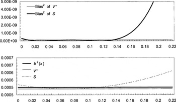
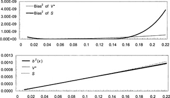
From Figures 1 and 2 one can conclude that in low/moderate values of interest rate both nonparametric estimators produce similar and good estimates whereas in high/very high values, the Sn estimates are generally worse than the Vn* estimates. We give a short explanation for these results. Coherently with most empirical studies of interest rate series, we observe the following pattern. In the interval of moderate/low values not only is the volatility very low but also the process displays martingale behavior, in the sense that a(x) ≈ 0 for x belonging to the interval of moderate/low values. In this interval, the asymptotic bias of Sn (and also of Vn*) is in general very low. By contrast, in the interval of high/very high values of interest rates, the volatility increases significantly and the process exhibits stronger reversion effects. It is in this interval, where |a(x)| is higher, that Sn produces greater bias and, simultaneously, that Vn* shows significant improvement over Sn.

Behavior of the S and V* estimators (as n → +∞) when and the model is dXt = 0.261(0.0717 − Xt) dt + 0.02237dWt.

Behavior of the S and V* estimators (as n → +∞) when and the model is .
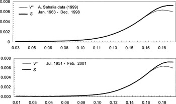
It is now interesting to compare the Sn and Vn* estimates for the diffusion coefficient using the Fed fund data referred to previously.
From Figure 3 it seems that the volatility at high values of interest rate, although considerable, is not as great as the Sn estimator suggests. However, no definitive conclusions can be made because in the areas where the drift coefficient is substantially negative (high in absolute value) there are not sufficient observations to draw precise statistical inference (for a discussion on this topic, see Bandi, 2002).

Nonparametric diffusion estimation—Fed fund data.
Let us consider a slight increase in the parameters of the preceding models associated with the reversion effects (everything else remains unchanged):

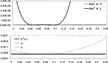
(in both cases, the parameter β defined in the drift function a(x) = β(μ − x) has changed to 0.9). Although these models certainly no longer reflect the behavior of the interest rate process, they allow us to appreciate the advantages of the proposed estimator when stronger reversion effects characterize the dynamics of the conditional mean. In fact, as can be seen from Figures 4 and 5, greater improvement is achieved by the Vn* estimates over the Sn estimates.

Behavior of the S and V* estimators (as n → +∞) when and the model is dXt = 0.9(0.0717 − Xt)dt + 0.02237dWt.

Behavior of the S and V* estimators (as n → +∞) when and the model is .
5. CONCLUSIONS AND OTHER EXTENSIONS
In this paper, we quantified the asymptotic bias of the Florens-Zmirou (1993) and Jiang and Knight (1997) estimator for the diffusion coefficient when the step of discretization is fixed, and subsequently we proposed a bias adjustment that partially compensates for the distortion. Also, we showed that our estimators have all the asymptotic properties of the Florens-Zmirou and Jiang and Knight estimator when the step of discretization goes to zero. There are some improvements that can be considered. First, more general assumptions on the data generator process as in Bandi and Phillips (2003) can in principle be applied. Second, other drift estimators can be considered, instead of Tn. For instance, the Jiang and Knight (1997) drift estimator can be used once one has a preliminary estimate of the diffusion estimator. Subsequently, an iterative procedure can be applied. I conjecture that the asymptotic properties of the Jiang and Knight drift estimator, with Δ fixed, can be improved if one uses the Vn* estimates instead of the Sn estimates. Third, a more accurate estimator for b2(x) can, in principle, be designed through the identification of the f (x) function using standard methods for derivative estimation, albeit at a natural cost of a reduction in the rates of convergence. Fourth, as in the case of the diffusion estimator, similar bias adjustments can be designed for the usual drift estimator Tn. Fifth, an evaluation of the bias produced by other nonparametric estimators (in the case Δn = Δ constant) such as the local linear or local quadratic regression can be analyzed (see Fan and Yao, 1998).
APPENDIX A: PRELIMINARY RESULTS
LEMMA 7 (Florens-Zmirou, 1989). Assume that

(

is the space of k times continuously differentiable functions). Then,

where L = a(d/dx) + ½b2(d2/dx2) and

See Hansen and Scheinkman (1995) for additional discussion. We assume in all applications involving Lemma 7 that

For example, if |Ls+1f (x)| ≤ k1(1 + x2r) holds for k1 > 0 and if, for some integer r > 0, we have E [Xt2r|Xs] ≤ (1 + |Xs2r|)eA(t−s) for A > 0, then E [|Ls+1f (Xti−1+us+1)||Xti−1] < +∞ (these conditions are generally easy to satisfy). It is worth mentioning that R depends on Xti−1 and Δs+1. We denote R by R = O(Δs+1).
The next lemmas deal with a central limit theorem version for discrete time processes {Xti, i ≥ 0} extracted from the diffusion process {Xt; t ≥ 0}.
LEMMA 8 (Florens-Zmirou, 1989). Let A1–A4 hold. Let

such that E [f (X)] = 0 and E [f2(X)] < +∞ where the expected values are evaluated with respect to the invariant distribution P0. Then

where

.
(We note that our A4 condition implies the H* condition defined in Florens-Zmirou, 1989.)
LEMMA 9 (Florens-Zmirou, 1989). Let

such that E [g(Xti−1,Xti)] = 0 and E [g2(Xti−1,Xti)] < +∞ where the expected values are evaluated with respect to the invariant distribution P0. Then

where

.
Note that

where y [map ] p(Δ,x,y) is the transition (or conditional) density of Xt+Δ given Xt = x and p is the stationary density. The following result is well known (see, e.g., Rao, 1983).
LEMMA 10. Let A1–A5 hold and hn → 0 and nhn → +∞ as n → +∞. Then

where

(

denotes convergence in MSE).
We discuss subsequently two distinct cases involving the estimator Bn. They are as follows: Δn → 0 and Δn = Δ constant as n → +∞. In both cases, Bn(x) is consistent in quadratic mean for p(x) provided that the other conditions in Lemma 10 are satisfied. We stress that the convergence of the density estimator in the presence of a constant Δ requires an increasing span tn.
APPENDIX B: PROOFS
The arguments we use to prove theorems in this Appendix differ from those of Florens-Zmirou (1993) and Jiang and Knight (1997) in that we do not consider an expansion of transition density.
Proof of Theorem 1. Let Sn(x) = An(x)/Bn(x) where

Given Lemma 10, it is enough to prove that

. To simplify we write An instead of An(x). We have (with Δn = Δ)

(with the change of variable z = x − hnu). Using Lemma 7 (with Δn = Δ)

equation (B.1) can be written as

Considering hn → 0, ∫K(u) du = 1, and the fact that a, b, f, and p are continuous functions (these sort of arguments will be used throughout the proofs), one has

It is now necessary to prove Var[An] → 0. We have

where f*(Xti,Xti+1) = f (Xti,Xti+1) − E [f (Xti,Xti+1)] and

Note that E [(f*(Xti,Xti+1))2] = E [f2(Xti,Xti+1)] − (E [f (Xti,Xti+1)])2 and

By Lemma 7 it is possible to check that

In this way,

This expression is clearly finite. On the other hand,

is finite and tends to zero.
In conclusion, E [(f*(Xti,Xti+1))2] is finite because E [f2(Xti,Xti+1)] is finite and E [f (Xti,Xti+1)] tends to zero. Then, by Lemma 9,

, and so

. Therefore,

and

because

by Lemma 10. █
The proofs of Theorems 2 and 3 are similar to the proof of Theorem 1 and thus are omitted.
Proof of Theorem 4. Let Vn*(x) = An*(x)/Bn(x) where

To simplify we write An* instead of An*(x). We first note that (with Δn = Δ)

To simplify we write D1,n and D2,n instead of D1,n(x) and D2,n(x), respectively. We now need the following result:

. Pointwise convergence,

(Theorem 3), does not imply

(see Davidson, 1994, Ch. 21). From Theorem 21.6 of Davidson (1994), suitably adapted to our problem, if Tn(x) converges in probability to a(x) + O(Δ) uniformly on an open set containing all the possible values of Xt, then it follows that

. In principle, the uniform convergence must hold in

although, in practice, because X is stationary, it is enough to take an open set V contained in some compact set V such that P(X ∈ V) = 1. Following Davidson (1994), Theorem 21.9, Tn(x) converges in probability to a(x) uniformly on a set V if and only if

for each x ∈ V and Tn(x) is stochastically equicontinuous. To guarantee this last condition, it is sufficient that supx∈V|dTn(x)/dx| be bounded in probability (Davidson, 1994, Theorem 21.10). Under the conditions established (note that we imposed that the kernel function and the infinitesimal coefficients are continuously differentiable) it follows that

, i.e., Tn(Xt) = a(Xt) + O(Δ) + εn, where εn = op(1). Thus,

We have (with Δn = Δ)

Using Lemma 7 (with Δn = Δ),

and the hypothesis hn → 0, one has lim E [D1,n] = O(Δ3). To prove Var[D1,n] → 0 we follow the same arguments we used in previous proofs; i.e., we define

where f*(Xti,Xti+1) = f (Xti,Xti+1) − E [f (Xti,Xti+1)] and

Using Lemma 7 one concludes

and using Lemma 9 and Assumption A5 we have lim Var[D1,n] = 0 and thus

.
Also, it is easy to see that

converges in probability to O(Δ3) (note that by Slutsky's theorem

. It follows from

, Theorem 2, and Lemma 10 that

. █
Proof of Theorem 5.
(a) Let Vn(x) = An#(x)/Bn(x) where

Given Lemma 10, it is enough to prove that

. From the proof of Theorem 1 it is straightforward to verify that

as Δn → 0, hn → 0, and nhn → +∞. Therefore,

. Let us see the second part of the theorem.
(b) To simplify we use the notation Ei [·] = E [·|Xti], and we write Σ instead of

. We note that

First, we show the following:

In effect,
(b1) applying Lemma 7 we have

Thus,

and

(using the change of variable, z = x − hnu, and Taylor's formula, b2(x − hnu) − b2(x) = O(hn)(b2(x − θhnu))′, with 0 < θ < 1). Therefore,

under the conditions of the theorem.
(b2) By Lemma 7,

Thus

and

With n → +∞, hn → 0, and Δn → 0 we have

(b3) We first show lim E [g(Xt0,Xt1)g(Xt1,Xt2)] = 0. Given

we have by Lemma 7

and, finally,

Hence, with hn → 0 and Δn → 0 (as n → +∞), we get

We now show lim E [g(Xt0,Xt1)g(Xtj,Xtj+1)] = 0 for j ≥ 1. By Assumption A4, the jth autocovariance of any function (square P0-integrable) tends to zero at exponential rate as j → +∞; thus, for j ≥ 1,

Given (B.3) and (B.4) we get (b3).
According to Lemma 9 (also see Florens-Zmirou, 1989, Theorem 3) we have

and thus (after standardization)

. Using the asymptotic equivalence theorem,

and

have the same asymptotic distribution, and thus the result is proved. █
Proof of Theorem 6.
(a) Let Vn*(x) = An*(x)/Bn(x) where

In the proof of Theorem 4 we saw that An*(x) can be written as An* = An# + D1,n + D2,n. A crucial step in this proof is that

as Δn → 0 and n → +∞. The estimator Tn(x) does not converge to a(x) as Δn → 0 unless we assume tn hn → +∞, thereby tn → +∞ (see also Bandi and Phillips, 2003). With the conditions stated one has

and even

, i.e., Tn(Xt) = a(Xt) + εΔn,n, where plimΔn→0,n→+∞ εΔn,n = 0 (see the proof of Theorem 4). Hence,

It is straightforward to conclude that

because

and

under the assumptions stated (in fact, each term of the summation in (B.5) is of order op(1)). Using the same arguments, it is easy to verify that

converges in probability to zero (note that by Slutsky's theorem

.
(b) First, note that

Now

because

(by hypothesis) and

These results are obvious and their proofs are omitted. It remains to observe that b−2(x)(2K2 Bn(x))−1/2 converge in probability to b−2(x)(2K2 p(x))−1/2. Therefore, the result (b) follows from Theorem 5. █
References
REFERENCES
Aït-Sahalia, Y.
(1996)
Nonparametric pricing of interest rate derivative securities.
Econometrica
64,
527–560.Google Scholar
Aït-Sahalia, Y.
(1999)
Transition densities for interest rate and other nonlinear
diffusions.
Journal of Finance
54,
1361–1395.Google Scholar
Andersen, T.,
T. Bollerslev,
F. Diebold, &
P. Labys
(2001)
The distribution of realized exchange rate volatility.
Journal of the American Statistical Association
96,
42–51.Google Scholar
Arnold, L.
(1974)
Stochastic Differential Equations: Theory and Application.
New York:
Wiley.
Bandi, F.
(2002)
Short-time interest rate dynamics: A spatial approach.
Journal of Financial Economics
65,
73–110.Google Scholar
Bandi, F. &
P. Phillips
(2003)
Fully nonparametric estimation of scalar diffusion models.
Econometrica
71,
241–283.Google Scholar
Brown, B. &
J. Hewitt
(1975)
Asymptotic likelihood theory for diffusion processes.
Journal of Applied Probability
12,
228–238.Google Scholar
Chen, X.,
L. Hansen, &
M. Carrasco
(1998)
Nonlinearity and Temporal Dependence.
Working paper.
Davidson, J.
(1994)
Stochastic Limit Theory.
Oxford, UK:
Oxford University Press.
Fan, J. &
Q. Yao
(1998)
Efficient estimation of conditional variance functions in
stochastic regression.
Biometrika
85,
645–660.Google Scholar
Florens-Zmirou, D.
(1989)
Approximate discrete-time schemes for statistics of diffusion
processes.
Statistics
4,
547–557.Google Scholar
Florens-Zmirou, D.
(1993)
On estimating the diffusion coefficient from discrete observation.
Journal of Applied Probability
30,
790–804.Google Scholar
Hansen, L. &
J. Scheinkman
(1995)
Back to the future: Generating moment implications for
continuous-time Markov processes.
Econometrica
63,
767–804.Google Scholar
Hansen, L.,
J. Scheinkman, &
N. Touzi
(1998)
Spectral methods for identifying scalar diffusions.
Journal of Econometrics
86,
1–32.Google Scholar
Ikeda, N. &
S. Watanabe
(1981)
Stochastic Differential Equations and Diffusion Processes.
North-Holland Mathematical Library.
Amsterdam: North-Holland.
Jiang, G. &
J. Knight
(1997)
A nonparametric approach to the estimation of diffusion processes,
with an application to a short-term interest rate model.
Econometric Theory
13,
615–645.Google Scholar
Karlin, S. &
H. Taylor
(1981)
A Second Course in Stochastic Processes.
New York:
Academic Press.
Merton, R.
(1990)
Continuous-Time Finance.
Oxford, UK:
Blackwell.
Phillips, P. &
J. Yu
(2000)
Exact Gaussian Estimation of Continuous Time Models of the Term
Structure of Interest Rates.
Working paper,
Yale University.
Rao, B.
(1983)
Nonparametrical Functional Estimation.
New York:
Academic Press.
Rao, B.
(1999)
Statistical Inference for Diffusion Type Processes.
New York:
Oxford University Press.
Sawyer, K.
(1993)
Continuous Time Financial Models: Statistical Applications of
Stochastic Processes. In
G. Maddala,
C. Rao,
H. Vinod (eds.),
Handbook of Statistics, pp.
573–610.
Amsterdam:
Elsevier Science Publishers.
Skorokhod, A.
(1989)
Asymptotic Methods in the Theory of Stochastic Differential
Equations,
Translation of Mathematical Monographs 78.
Providence, RI:
American Mathematical Society.
Stanton, R.
(1997)
A nonparametric model of term structure dynamics and the market
price of interest rate risk.
Journal of Finance
52,
1973–2000.Google Scholar
Behavior of the S and V* estimators (as n → +∞) when and the model is dXt = 0.261(0.0717 − Xt) dt + 0.02237dWt.
Behavior of the S and V* estimators (as n → +∞) when and the model is .
Nonparametric diffusion estimation—Fed fund data.
Behavior of the S and V* estimators (as n → +∞) when and the model is dXt = 0.9(0.0717 − Xt)dt + 0.02237dWt.
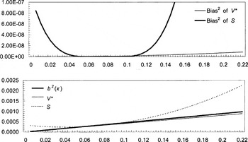
Behavior of the S and V* estimators (as n → +∞) when and the model is .
 You have
Access
- 31
- Cited by