1 Introduction
When examined at a nano- or microscopic scale, material surfaces cannot be considered perfectly smooth. Asperities and irregularities at various scales actually participate in conferring specific properties on such surfaces, as proved by examples taken from the vegetal or animal kingdom, e.g. the superhydrophobic properties of Salvinia molesta leaves (Tricinci et al.
Reference Tricinci, Terencio, Mazzolai, Pugno, Greco and Mattoli2015), the effect of dermal denticles on the swimming properties of sharks (Oeffner & Lauder Reference Oeffner and Lauder2012), the role of comb- and fringe-like feathers in the silent flight of owls (Lilley Reference Lilley1998) or that of scales of butterfly wings upon their flying efficiency (Slegers et al.
Reference Slegers, Heilman, Cranford, Lang, Yoder and Hebegger2017). The detailed study of non-smooth surfaces is a subject of growing importance that has given rise to several reviews, e.g. Rothstein (Reference Rothstein2010) and Bhushan & Jung (Reference Bhushan and Jung2011). An important branch of this topic emerged over the last two decades as a consequence of the background accumulated on hydro- and aerodynamical drag reduction via the use of the so-called riblets (Walsh Reference Walsh1983; Bechert & Bartenwerfer Reference Bechert and Bartenwerfer1989; Luchini, Manzo & Pozzi Reference Luchini, Manzo and Pozzi1991). Because of the separation of scales between the size of the riblets and the flow structures which appear above them, direct numerical simulations (DNS) can be prohibitively expensive in such configurations. Consequently, the Navier slip condition (Navier Reference Navier1823) has been widely used to simulate fluid flows over micro-structured walls. Actually, this boundary condition was not initially designed to deal with rough surfaces. In his 1823 seminal paper, Navier proposed the slip condition to close the flow governing equations on the sole basis of experimental considerations about the interaction between fluid particles and a generic solid wall. This condition involves a constant,
 $\unicode[STIX]{x1D706}$
, today called the slip length, which depends on the physical properties of the fluid and the wall. No further considerations about
 $\unicode[STIX]{x1D706}$
were made by Navier, for whom it was clear that only physical measurements could unveil additional information. In the last two decades, the Navier slip condition has been widely used in applications connected primarily with superhydrophobic surfaces (Ybert, Barentin & Cottin-Bizonne Reference Ybert, Barentin and Cottin-Bizonne2007; Cottin-Bizonne, Barentin & Bocquet Reference Cottin-Bizonne, Barentin and Bocquet2012). Surface roughness is one of the main ingredients of superhydrophobicity through the gas plastron which remains trapped within the rough layer, producing a decrease of the frictional stress acting on the fluid (Onda et al.
Reference Onda, Shibuichi, Satoh and Tsujii1996). Without the micro-roughnesses, the gas would not adhere to the surface and the hydrophobic effect would be significantly reduced. Much effort has been devoted to the theoretical characterization of
 $\unicode[STIX]{x1D706}$
, both with and without a gas plastron (Luchini et al.
Reference Luchini, Manzo and Pozzi1991; Lauga & Stone Reference Lauga and Stone2003; Lauga, Brenner & Stone Reference Lauga, Brenner, Stone, Foss, Tropea and Yarin2005; Davis & Lauga Reference Davis and Lauga2010).
Besides these classical applications related to external flows, there is a rapidly growing interest for fluid flows at the nanoscale, driven by the technological evolutions that render the fabrication of nano-devices possible. Some applications of carbon nanotubes, which exhibit exceptional and tuneable hydrodynamical (Majumder et al. Reference Majumder, Chopra, Andrews and Hinds2005), optical and electrical properties (De Nicola et al. Reference De Nicola, Castrucci, Scarselli, Nanni, Cacciotti and De Crescenzi2015) are found in water desalination (Goh, Ismail & Ng Reference Goh, Ismail and Ng2009) and drug delivery, aimed at killing cancer cells (Bhirde et al. Reference Bhirde, Patel, Gavard, Zhang, Sousa, Masedunskas, Leapman, Weigert, Gutkind and Rusling2009).
The above context suggests that reconsidering the Navier slip condition to develop a model capable of predicting consistently the microscopic slip for a generic micro-structured surface is in order. A recent step towards this direction was performed by Jiménez Bolaños & Vernescu (Reference Jiménez Bolaños and Vernescu2017) who re-derived the Navier relation by using a homogenization technique in the small roughness case, as defined by Luchini (Reference Luchini2013). Small roughness means that the rough surface has the form
 $\hat{x}_{3}=\unicode[STIX]{x1D716}h(\hat{x}_{1}/\unicode[STIX]{x1D716},\hat{x}_{2}/\unicode[STIX]{x1D716})$
(cf. figure 1), i.e. the surface remains geometrically similar to itself when
 $\unicode[STIX]{x1D716}\rightarrow 0$
. The other significant limit discussed by Luchini (Reference Luchini2013) is the shallow roughness case,
 $\hat{x}_{3}=\unicode[STIX]{x1D716}h(\hat{x}_{1},\hat{x}_{2})$
, for which the surface becomes flatter and flatter as
 $\unicode[STIX]{x1D716}\rightarrow 0$
. In both instances, the tangential velocity components at a virtual wall can be cast in the form of a Navier slip condition with a slip length provided either by the solution of microscopic closure problems (Jiménez Bolaños & Vernescu Reference Jiménez Bolaños and Vernescu2017) or by the direct boundary integral solution of the Stokes equation (Luchini Reference Luchini2013). In the latter case, also a proximity coefficient was defined and computed, to be used whenever interactions among densely spaced wall protuberances become important (for an earlier analysis see Sarkar & Prosperetti Reference Sarkar and Prosperetti1996). The shallow limit was also considered by Kamrin, Bazant & Stone (Reference Kamrin, Bazant and Stone2010) by a perturbative expansion in
 $\unicode[STIX]{x1D716}$
carried out to second order; the result is an approximate mobility tensor which relates the slip velocity to the mean surface traction. A mobility tensor, which in the present paper will be called the Navier slip tensor or simply the slip tensor and, in the study of riblets, was named the protrusion tensor, see Bechert & Bartenwerfer (Reference Bechert and Bartenwerfer1989) and Luchini et al. (Reference Luchini, Manzo and Pozzi1991), had been previously introduced by Bazant & Vinogradova (Reference Bazant and Vinogradova2008) and justified also on the basis of molecular arguments; the main scope of their paper was to illustrate the power of the tensorial formalism in capturing complex effects related to the presence of anisotropic textured surfaces. Effective boundary conditions for momentum and heat transfer at rough walls, where the microscopic properties of the surfaces are transferred to an effective condition by solving closure problems at a microscopic level, have also been developed in the framework of the volume averaging method (Veran, Aspa & Quintard Reference Veran, Aspa and Quintard2009; Introïni, Quintard & Duval Reference Introïni, Quintard and Duval2011; Guo, Veran-Tissoires & Quintard Reference Guo, Veran-Tissoires and Quintard2016; Pasquier, Quintard & Davit Reference Pasquier, Quintard and Davit2017).
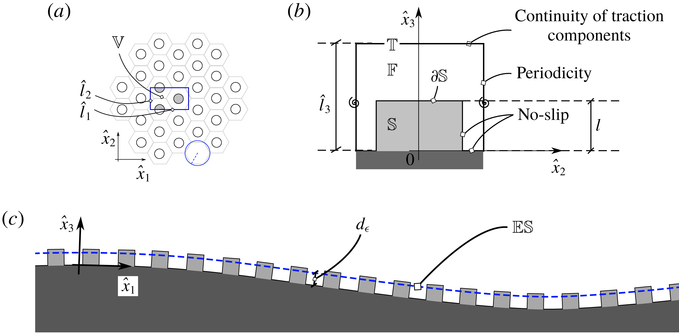
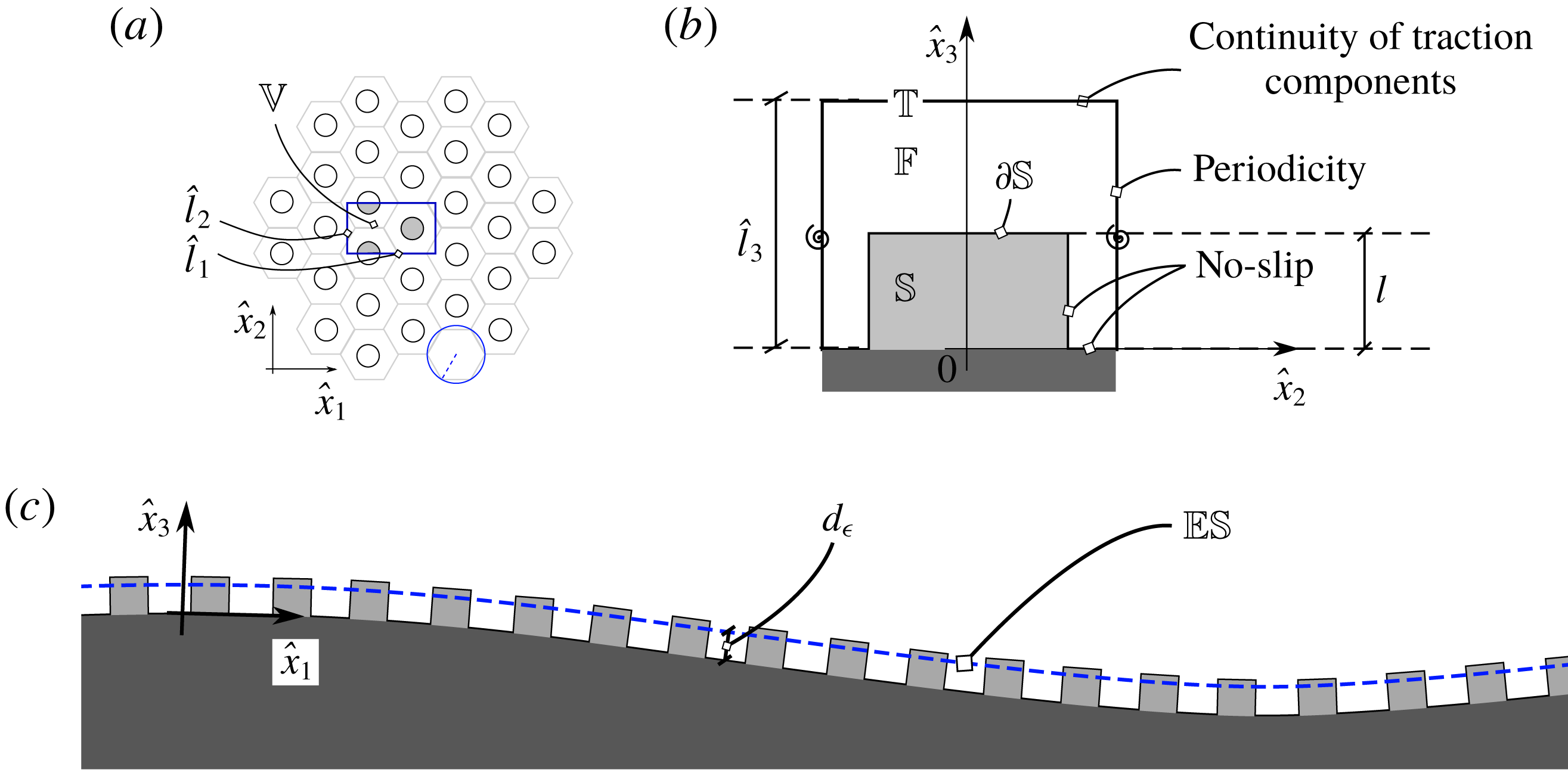
Views of the rough surface under investigation. (a) Top view of a hexagonal periodic lattice on a surface. The microscopic unit cell
 $\mathbb{V}$
(blue rectangle online), formed by a fluid region
 $\mathbb{F}$
and a solid region
 $\mathbb{S}$
, the common boundary of which is
 $\unicode[STIX]{x2202}\mathbb{S}$
, as seen in (b), has tangential dimensions equal to
 $\hat{l}_{1}$
and
 $\hat{l}_{2}$
, respectively, both of order
 $l$
. The position of the top of the cell,
 $\mathbb{T}$
, defines the height of the latter,
 $\hat{l}_{3}$
, which must also be of order
 $l$
(this corresponds to the so-called small roughness limit of Luchini (Reference Luchini2013)). (b) Cut of the microscopic cell, at a fixed
 $\hat{x}_{1}$
through the centre of the protrusion. (c) Cut of the macroscopic rough surface at a fixed
 $\hat{x}_{2}$
. The fictitious equivalent surface
 $\mathbb{ES}$
is represented by a dashed line (blue online).
As mentioned above, developing an accurate macroscopic framework remains fully relevant nowadays, given the computational costs required to simulate microscale flow phenomena and the huge separation of scales encountered in many applications. A considerable amount of computational resources can be saved if a proper macroscopic condition is imposed on an equivalent smooth surface to simulate the influence of roughness on the large-scale flow, provided that only local fluid motions of minor significance are not captured. In the present work, a multiscale homogenization technique, similar to that used by Jiménez Bolaños & Vernescu (Reference Jiménez Bolaños and Vernescu2017), is employed to link the macroscopic and microscopic viewpoints. Since the phenomena under investigation are inhomogeneous in the direction normal to the surface, the standard homogenization technique needs to be adapted through a procedure similar to that followed by Lācis & Bagheri (Reference Lācis and Bagheri2017) and Lācis, Zampogna & Bagheri (Reference Lācis, Zampogna and Bagheri2017). The outcome of this approach is a boundary condition which extends the Navier slip concept and contains in itself the formulation and boundary conditions of the microscopic problems to determine the general relationship between the outer flow characteristics (more specifically the various components of the strain rate) and the geometry of the rough layer. Jiménez Bolaños & Vernescu (Reference Jiménez Bolaños and Vernescu2017) mention than their approach can be extended to three-dimensional flows. However, only two-dimensional configurations are actually considered throughout their paper. Here this extension is carried out and applied to a fully three-dimensional configuration. Hence, the boundary condition derived below is directly applicable to an arbitrarily shaped macroscopic surface.
Section 2 presents the derivation of the generalized Navier boundary condition, highlighting the main steps of the homogenization approach together with the underlying assumptions. The generalized boundary condition, initially developed in local surface-dependent coordinates in § 2, is extended to global Cartesian coordinates in appendix A. The condition is developed under the hypothesis that the local (roughness-based) Reynolds number is small. The components of the slip tensor are computed and discussed in § 3. In § 4, we describe the configuration chosen to validate the homogenized model, consisting of a sphere coated with a hexagonal lattice of cylinders. We have paid special attention to the coating design in order to obtain a quasi-isotropic coverage. The results of the fully resolved simulations used later to validate the developed model are presented in this section. In § 5 we apply the generalized boundary condition to compute the flow in the chosen configuration at regimes of moderate-to-large Reynolds numbers. We then compare the solutions provided by the macroscopic approach with those of the fully resolved simulations, in laminar and turbulent regimes. This allows us to highlight the pros and cons of the boundary condition in terms of the flow regime. A summary of the main findings of the paper and avenues for future research directions are provided in § 6.
2 An effective boundary condition for rough surfaces
We consider an incompressible Newtonian fluid of constant density
 $\unicode[STIX]{x1D70C}$
and viscosity
 $\unicode[STIX]{x1D707}$
, flowing above a rough surface
 $\mathbb{S}$
as sketched in figure 1. The velocity and pressure fields in the fluid domain
 $\mathbb{F}$
are governed by the Navier–Stokes equations
 $$\begin{eqnarray}\displaystyle & \displaystyle \unicode[STIX]{x1D70C}\frac{\unicode[STIX]{x2202}\hat{u} _{i}}{\unicode[STIX]{x2202}\hat{t}}+\unicode[STIX]{x1D70C}\hat{u} _{j}\frac{\unicode[STIX]{x2202}\hat{u} _{i}}{\unicode[STIX]{x2202}\hat{x}_{j}}=-\frac{\unicode[STIX]{x2202}\hat{p}}{\unicode[STIX]{x2202}\hat{x}_{i}}+\unicode[STIX]{x1D707}\hat{\unicode[STIX]{x1D6FB}}^{2}\hat{u} _{i}, & \displaystyle\end{eqnarray}$$
 $$\begin{eqnarray}\displaystyle & \displaystyle \frac{\unicode[STIX]{x2202}\hat{u} _{i}}{\unicode[STIX]{x2202}\hat{x}_{i}}=0, & \displaystyle\end{eqnarray}$$
with
 $\hat{u} _{i}=0$
on the solid–fluid boundary
 $\unicode[STIX]{x2202}\mathbb{S}$
. The roughness of the surface is provided by the presence of small protrusions distributed on a smooth surface; they are such that the surface geometry is characterized by a large separation of scales between the size
 $L$
of the large-scale flow structures and the size
 $l$
of the protrusions. In other words, the parameter
 $\unicode[STIX]{x1D716}$
satisfies the typical relation
 $$\begin{eqnarray}\unicode[STIX]{x1D716}=\frac{l}{L}\ll 1.\end{eqnarray}$$
The particular arrangement of the protrusions (which are assumed to have a fixed shape) forms a periodic tessellation of the surface. Due to the large separation of scales, the effect of the macroscopic curvature is negligible from a microscopic point of view and the flow can thus be assumed to be periodic over the cell
 $\mathbb{V}=\mathbb{F}\cup \mathbb{S}$
.
As we explain below, using (2.3) makes it possible to approximate the rough surface by an equivalent smooth surface
 $\mathbb{ES}$
, located a certain distance
 $d_{\unicode[STIX]{x1D716}}$
from the smooth, possibly curved, surface over which the protrusions are placed (the smooth surface bounds the dark grey region shown in figure 1
c);
 $d_{\unicode[STIX]{x1D716}}$
is of
 $O(l)$
and is unspecified a priori. We define the inner region (or rough layer) as the portion of space located between the surface and
 $\mathbb{T}$
, and the outer region as the portion of space standing beyond
 $\mathbb{T}$
. Note that
 $\mathbb{ES}$
does not necessarily separate the inner and outer regions, i.e. it does not in general coincide with
 $\mathbb{T}$
. From the point of view of homogenization,
 $\mathbb{ES}$
represents the homogeneous surface (i.e. a region without any distinction of phases) where macroscopic conditions can be applied. In this case, the resulting interface relation is a slip condition for the velocity field.
We proceed to develop the boundary condition by applying a homogenization technique to the flow in the inner region, and then imposing the continuity of velocity and traction with the outer region at
 $\mathbb{T}$
. This procedure is similar to that employed by Lācis & Bagheri (Reference Lācis and Bagheri2017) to develop a condition to be imposed at the interface between a free fluid region and a homogeneous porous region, but it yields different results because of differences in the relevant scales, as explained later on. We consider only the fluid region within the unit cell (
 $\mathbb{F}$
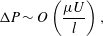
). To normalize the equations in this region, we assume that the pressure variation within the inner region is such that
 $$\begin{eqnarray}\unicode[STIX]{x0394}P\sim O\left(\frac{\unicode[STIX]{x1D707}U}{l}\right),\end{eqnarray}$$
i.e.
 $\unicode[STIX]{x0394}P$
is of the order of the stress imposed at the upper microscopic boundary
 $\mathbb{T}$
of the unit cell, as in Kamrin et al. (Reference Kamrin, Bazant and Stone2010). The scaled dimensionless variables are related to the dimensional ones through
 $$\begin{eqnarray}\hat{t}=\frac{l}{U}t=\frac{\unicode[STIX]{x1D707}}{\unicode[STIX]{x0394}P}t,\quad \hat{\boldsymbol{x}}=l\boldsymbol{x},\quad \hat{p}=\unicode[STIX]{x0394}Pp,\quad \hat{\boldsymbol{u}}=U\boldsymbol{u}=\frac{l\unicode[STIX]{x0394}P}{\unicode[STIX]{x1D707}}\boldsymbol{u}.\end{eqnarray}$$
The governing equations in
 $\mathbb{F}$
thus become
 $$\begin{eqnarray}\displaystyle & \displaystyle \frac{\unicode[STIX]{x2202}u_{i}}{\unicode[STIX]{x2202}x_{i}}=0, & \displaystyle\end{eqnarray}$$
 $$\begin{eqnarray}\displaystyle & \displaystyle Re\left(\frac{\unicode[STIX]{x2202}u_{i}}{\unicode[STIX]{x2202}t}+u_{j}\frac{\unicode[STIX]{x2202}u_{i}}{\unicode[STIX]{x2202}x_{j}}\right)=-\frac{\unicode[STIX]{x2202}p}{\unicode[STIX]{x2202}x_{i}}+\unicode[STIX]{x1D6FB}^{2}u_{i}, & \displaystyle\end{eqnarray}$$
where
 $Re$
is the microscale Reynolds number, defined as
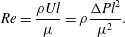 $$\begin{eqnarray}Re=\frac{\unicode[STIX]{x1D70C}Ul}{\unicode[STIX]{x1D707}}=\unicode[STIX]{x1D70C}\frac{\unicode[STIX]{x0394}Pl^{2}}{\unicode[STIX]{x1D707}^{2}}.\end{eqnarray}$$
Since our goal is to develop macroscopic boundary conditions that account for the presence of the protrusions, we need to consider also the flow outside the rough layer. In this outer region, the relevant length scale is the macroscopic one,
 $L$
. Denoting non-dimensional quantities in this external region (located beyond the top
 $\mathbb{T}$
of each cell) with the superscript
 $^{out}$
, we have
 $$\begin{eqnarray}\hat{t}=\frac{L}{U^{out}}t^{out}=\unicode[STIX]{x1D716}\frac{L}{U}t^{out}=\frac{l}{U}t,\quad \hat{\boldsymbol{x}}=L\boldsymbol{x}^{out},\quad \hat{p}=\unicode[STIX]{x0394}Pp^{out},\quad \hat{\boldsymbol{u}}=\frac{U}{\unicode[STIX]{x1D716}}\boldsymbol{u}^{out}=\frac{L\unicode[STIX]{x0394}P}{\unicode[STIX]{x1D707}}\boldsymbol{u}^{out},\end{eqnarray}$$
where lengths are normalized with the macroscopic scale
 $L$
. We have assumed that the velocity scale in the outer region,
 $U^{out}$
, is
 $1/\unicode[STIX]{x1D716}$
times larger than the velocity scale
 $U$
within the rough layer; this is consistent with the fact that the inner–outer problem is coupled through a unique time scale,
 $l/U$
. These normalizations will be used later to infer boundary conditions for the microscale problem.
For the sake of simplicity, we develop the model in local coordinates for surfaces covered by a lattice of hexagonal periodic cells. In this case, the pattern is periodic along the directions
 $\hat{x}_{1}$
and
 $\hat{x}_{2}$
tangential to the plane. Figure 1 indicates that the flow characteristics only experience slow variations in these directions, but may vary much faster in the
 $\hat{x}_{3}$
direction normal to the plane. For this reason, within the rough layer, we can use the multiscale homogenization approach described by Mei & Vernescu (Reference Mei and Vernescu2010); we introduce the fast (microscopic) and slow (macroscopic) variables,
 $\boldsymbol{x}=(x_{1},x_{2},x_{3})$
and
 $\boldsymbol{x}^{\prime }=\unicode[STIX]{x1D716}(x_{1},x_{2})$
, and the expansions
 $$\begin{eqnarray}\boldsymbol{u}=\boldsymbol{u}^{(0)}+\unicode[STIX]{x1D716}\boldsymbol{u}^{(1)}+\cdots \,,\quad p=p^{(0)}+\unicode[STIX]{x1D716}p^{(1)}+\cdots \,,\end{eqnarray}$$
where
 $\boldsymbol{u}^{(i)}$
and
 $\boldsymbol{p}^{(i)}$
are functions of
 $(\boldsymbol{x},\boldsymbol{x}^{\prime },t)$
. Noting that
 $$\begin{eqnarray}\frac{\unicode[STIX]{x2202}}{\unicode[STIX]{x2202}x_{i}}\rightarrow \frac{\unicode[STIX]{x2202}}{\unicode[STIX]{x2202}x_{i}}+\unicode[STIX]{x1D716}\frac{\unicode[STIX]{x2202}}{\unicode[STIX]{x2202}x_{i}^{\prime }}\quad \text{for }i=1,2,\end{eqnarray}$$
substituting (2.10) into the Navier–Stokes equations and collecting terms at every order in
 $\unicode[STIX]{x1D716}$
, we obtain at leading order
 $$\begin{eqnarray}\displaystyle & \displaystyle \frac{\unicode[STIX]{x2202}u_{i}^{(0)}}{\unicode[STIX]{x2202}x_{i}}=0\quad \forall i, & \displaystyle\end{eqnarray}$$
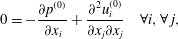 $$\begin{eqnarray}\displaystyle & \displaystyle 0=-\frac{\unicode[STIX]{x2202}p^{(0)}}{\unicode[STIX]{x2202}x_{i}}+\frac{\unicode[STIX]{x2202}^{2}u_{i}^{(0)}}{\unicode[STIX]{x2202}x_{j}\unicode[STIX]{x2202}x_{j}}\quad \forall i,\forall \,j, & \displaystyle\end{eqnarray}$$
under the hypothesis that
 $Re$
is at most
 $O(\unicode[STIX]{x1D716})$
. With the chosen scalings, one can in principle define an outer Reynolds number
 $Re^{out}$
as
 $U^{out}L/\unicode[STIX]{x1D708}$
, a parameter which can formally be as large as
 $\unicode[STIX]{x1D716}^{-1}$
. It is however incorrect for the outer Reynolds number to depend on
 $\unicode[STIX]{x1D716}$
since, in applications, once the macroscopic geometry, the fluid viscosity and the pressure gradient are set, the flow speed to be used in the definition of
 $Re^{out}$
ensues. The point is that, in the theory,
 $Re$
and
 $Re^{out}$
are chained together by the need to take a distinguished limit, chosen here as
 $\unicode[STIX]{x1D716}\overset{\underset{\mathit{def}}{}}{=}l/L=O(Re)$
. However, once the boundary condition is derived, its validity is set by the value of
 $Re$
only. Should the actual value of
 $Re^{out}$
(based on some relevant macroscopic speed) be so large as to render the flow turbulent, we might end up in the so-called low range transitionally rough regime (Thakkar, Busse & Sandham Reference Thakkar, Busse and Sandham2018). Normalizing the roughness height,
 $k_{s}$
, by the friction velocity,
 $u_{\unicode[STIX]{x1D70F}}$
, and the kinematic viscosity,
 $\unicode[STIX]{x1D708}=\unicode[STIX]{x1D707}/\unicode[STIX]{x1D70C}$
, this regime corresponds to a dimensionless roughness height
 $k_{s}^{+}=k_{s}u_{\unicode[STIX]{x1D70F}}/\unicode[STIX]{x1D708}\lesssim 13$
. At variance with earlier beliefs (Schlichting Reference Schlichting1979), it is now established that within this range of
 $k_{s}^{+}$
, the logarithmic velocity profile in pipes or boundary layers experiences a non-zero shift,
 $\unicode[STIX]{x0394}U^{+}$
, in the form of a power law
 $\unicode[STIX]{x0394}U^{+}\sim {k_{s}^{+}}^{\unicode[STIX]{x1D6FC}}$
down to the smooth-wall limit,
 $k_{s}^{+}=0$
. Although Bradshaw (Reference Bradshaw2000) suggested
 $\unicode[STIX]{x1D6FC}=2$
on the basis of an analogy with the Oseen flow past a lattice of spheres, the recent DNS results by Thakkar et al. (Reference Thakkar, Busse and Sandham2018) obtained over a grit-blasted wall indicate
 $\unicode[STIX]{x1D6FC}\approx 1.37$
. Being based on Stokes’ approximation within the rough layer, the present theory cannot reproduce this small shift resulting from small inertial effects.
In contrast, this theory is well suited to approximate
 $\unicode[STIX]{x0394}U^{+}$
in the limit
 $Re\rightarrow 0$
when the individual roughness elements or the lattice they form are anisotropic (e.g. the riblets considered by Bechert & Bartenwerfer (Reference Bechert and Bartenwerfer1989) and Luchini et al. (Reference Luchini, Manzo and Pozzi1991)), a configuration in which
 $\unicode[STIX]{x0394}U^{+}$
results from a linear mechanism and is, to leading order, directly proportional to the difference between longitudinal and transverse protrusion heights (Luchini Reference Luchini, Choi, Prasad and Truong1992; García-Mayoral & Jiménez Reference García-Mayoral and Jiménez2011). However, in the specific case treated later in §§ 3 and 4, the selected lattice is isotropic and so is the resulting slip tensor; this translates into a normal shift of the whole equivalent mean surface
 $\mathbb{ES}$
and, because of the single virtual origin for all velocity components,
 $\unicode[STIX]{x0394}U^{+}$
vanishes at leading order.
In order to formally write the solution of (2.12) and (2.13), we need to consider the conditions imposed on the boundaries of
 $\mathbb{F}$
. As indicated in figure 1, periodicity holds along the tangential directions,
 $x_{1}$
and
 $x_{2}$
, whereas the no-slip condition
 $$\begin{eqnarray}\hat{u} _{i}^{(0)}=0\end{eqnarray}$$
holds at the common boundary,
 $\unicode[STIX]{x2202}\mathbb{S}$
, between
 $\mathbb{F}$
and
 $\mathbb{S}$
. At the top surface
 $\mathbb{T}$
of the microscopic cell (
 $x_{3}=l_{3}=\hat{l}_{3}/l$
), the continuity of tractions implies
 $$\begin{eqnarray}\hat{\unicode[STIX]{x1D61B}}_{jk}n_{k}|_{in}=\hat{\unicode[STIX]{x1D61B}}_{jk}n_{k}|_{out},\end{eqnarray}$$
where
 $\hat{\unicode[STIX]{x1D61B}}_{jk}=-\hat{p}\unicode[STIX]{x1D6FF}_{jk}+\unicode[STIX]{x1D707}(\unicode[STIX]{x2202}\hat{u} _{j}/\unicode[STIX]{x2202}\hat{x}_{k}+\unicode[STIX]{x2202}\hat{u} _{k}/\unicode[STIX]{x2202}\hat{x}_{j})$
is the dimensional stress tensor (calculated in the inner,
 $|_{in}$
, or outer,
 $|_{out}$
, region) and
 $n_{k}$
denotes the unit normal vector which, in the present case, corresponds to
 $\boldsymbol{e}_{3}$
. In outer scales, the fictitious surface
 $\mathbb{ES}$
corresponds to
 $x_{3}^{out}\rightarrow d_{\unicode[STIX]{x1D716}}/L$
. The dimensional outer spatial variable scales with
 $L$
, as the macroscopic variable in the inner region (thus
 $x_{i}^{out}=x_{i}^{\prime }$
for
 $i=1,2$
), but it is extended also along the third direction. Because of this, we are allowed to differentiate from the top towards the surface. Then, using (2.5) and (2.9) and considering only the leading-order terms, equation (2.15) implies
 $$\begin{eqnarray}\frac{\unicode[STIX]{x2202}u_{i}^{(0)}}{\unicode[STIX]{x2202}x_{3}}+\frac{\unicode[STIX]{x2202}u_{3}^{(0)}}{\unicode[STIX]{x2202}x_{i}}=\frac{\unicode[STIX]{x2202}u_{i}^{out}}{\unicode[STIX]{x2202}x_{3}^{out}}+\frac{\unicode[STIX]{x2202}u_{3}^{out}}{\unicode[STIX]{x2202}x_{i}^{\prime }}\quad i=1,2\end{eqnarray}$$
and
 $$\begin{eqnarray}-p^{(0)}+2\frac{\unicode[STIX]{x2202}u_{3}^{(0)}}{\unicode[STIX]{x2202}x_{3}}=-p^{out}+2\frac{\unicode[STIX]{x2202}u_{3}^{out}}{\unicode[STIX]{x2202}x_{3}^{out}}.\end{eqnarray}$$
Condition (2.16) is used later on to seek an appropriate form of
 $u_{i}^{(0)}$
; condition (2.17) can be employed to set the reference value for the pressure (see (2.20)). Continuity of velocities on
 $\mathbb{T}$
imposes
 $$\begin{eqnarray}\hat{u} _{i}^{(0)}=\hat{u} _{i}^{out},\end{eqnarray}$$
which, in dimensionless form, reads
 $\unicode[STIX]{x1D716}u_{i}^{(0)}=u_{i}^{out}$
. This condition simply states that the outer velocity vanishes at leading order. Owing to linearity, the solution of (2.12) and (2.13) may be written in the form
 $$\begin{eqnarray}\displaystyle & \displaystyle u_{i}^{(0)}=\unicode[STIX]{x1D613}_{il3}\left.\left(\frac{\unicode[STIX]{x2202}u_{l}^{out}}{\unicode[STIX]{x2202}x_{3}^{out}}+\frac{\unicode[STIX]{x2202}u_{3}^{out}}{\unicode[STIX]{x2202}x_{l}^{\prime }}\right)\right|_{x_{3}=l_{3}},\quad l=1,2,\,\,\forall \,i, & \displaystyle\end{eqnarray}$$
 $$\begin{eqnarray}\displaystyle & \displaystyle p^{(0)}-p_{0}(\boldsymbol{x}^{\prime })=\unicode[STIX]{x1D609}_{l3}\left.\left(\frac{\unicode[STIX]{x2202}u_{l}^{out}}{\unicode[STIX]{x2202}x_{3}^{out}}+\frac{\unicode[STIX]{x2202}u_{3}^{out}}{\unicode[STIX]{x2202}x_{l}^{\prime }}\right)\right|_{x_{3}=l_{3}}\quad l=1,2, & \displaystyle\end{eqnarray}$$
where
 $\unicode[STIX]{x1D613}_{il3}$
and
 $\unicode[STIX]{x1D609}_{l3}$
are unknown tensors and
 $p_{0}(\boldsymbol{x}^{\prime })$
is the reference pressure imposed by the outer flow through (2.17). Given the previous assumptions and boundary conditions, only a subset of the tensors’ components can be different from zero, namely
 $\unicode[STIX]{x1D613}_{113}$
,
 $\unicode[STIX]{x1D613}_{213}$
,
 $\unicode[STIX]{x1D613}_{313}$
,
 $\unicode[STIX]{x1D613}_{123}$
,
 $\unicode[STIX]{x1D613}_{223}$
,
 $\unicode[STIX]{x1D613}_{323}$
and
 $\unicode[STIX]{x1D609}_{13}$
,
 $\unicode[STIX]{x1D609}_{23}$
. Substituting (2.19) and (2.20) into (2.12) and (2.13), it is readily found that the non-zero components satisfy the problem
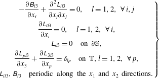 $$\begin{eqnarray}\left.\begin{array}{@{}c@{}}-{\displaystyle \frac{\unicode[STIX]{x2202}\unicode[STIX]{x1D609}_{l3}}{\unicode[STIX]{x2202}x_{i}}}+{\displaystyle \frac{\unicode[STIX]{x2202}^{2}\unicode[STIX]{x1D613}_{il3}}{\unicode[STIX]{x2202}x_{j}\unicode[STIX]{x2202}x_{j}}}=0,\quad l=1,2,\,\,\forall \,i,j\\ {\displaystyle \frac{\unicode[STIX]{x2202}\unicode[STIX]{x1D613}_{il3}}{\unicode[STIX]{x2202}x_{i}}}=0,\quad l=1,2,\,\,\forall \,i,\\ \unicode[STIX]{x1D613}_{il3}=0\quad \text{on }\unicode[STIX]{x2202}\mathbb{S},\\ {\displaystyle \frac{\unicode[STIX]{x2202}\unicode[STIX]{x1D613}_{pl3}}{\unicode[STIX]{x2202}x_{3}}}+{\displaystyle \frac{\unicode[STIX]{x2202}\unicode[STIX]{x1D613}_{3l3}}{\unicode[STIX]{x2202}x_{p}}}=\unicode[STIX]{x1D6FF}_{lp}\quad \text{on }\mathbb{T},l=1,2,\,\,\forall \,p,\\ \unicode[STIX]{x1D613}_{il3},\unicode[STIX]{x1D609}_{l3}\quad \text{periodic along the }x_{1}\text{ and }x_{2}\text{ directions.}\end{array}\right\}\end{eqnarray}$$
To ensure uniqueness of the solution of (2.21), we also impose
 $$\begin{eqnarray}\langle \unicode[STIX]{x1D609}_{j3}\rangle =0\end{eqnarray}$$
for
 $j=1,2$
, where the volume average over a unit cell,
 $\langle \cdot \rangle$
, is defined as
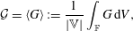 $$\begin{eqnarray}{\mathcal{G}}=\langle G\rangle :=\frac{1}{|\mathbb{V}|}\int _{\mathbb{F}}G\,\text{d}V,\end{eqnarray}$$
and
 $|\mathbb{V}|$
denotes the volume of
 $\mathbb{V}$
. Taking the volume average of (2.19), noting that
 $\boldsymbol{u}^{out}$
and
 $p_{0}$
do not depend on the fast variable
 $\boldsymbol{x}$
and making use of (2.22), we obtain
 $$\begin{eqnarray}\langle u_{i}^{(0)}\rangle ={\mathcal{L}}_{il3}\left.\left(\frac{\unicode[STIX]{x2202}u_{l}^{out}}{\unicode[STIX]{x2202}x_{3}^{out}}+\frac{\unicode[STIX]{x2202}u_{3}^{out}}{\unicode[STIX]{x2202}x_{l}^{\prime }}\right)\right|_{x_{3}^{out}\rightarrow d_{\unicode[STIX]{x1D716}}/L},\quad j,l=1,2,\,\,\forall \,i,\end{eqnarray}$$
with
 $$\begin{eqnarray}{\mathcal{L}}_{ij3}=\langle \unicode[STIX]{x1D613}_{ij3}\rangle .\end{eqnarray}$$
Furthermore, on averaging (2.20), we have
 $$\begin{eqnarray}\langle p^{(0)}\rangle =\frac{|\mathbb{F}|}{|\mathbb{V}|}p_{0}.\end{eqnarray}$$
It is important to notice that, after averaging (2.19), the microscopic domain has shrunk to a single point along the normal-to-the-surface direction, i.e.
 $x_{3}=l_{3}$
in (2.19) and (2.20) has become
 $x_{3}^{out}\rightarrow d_{\unicode[STIX]{x1D716}}/L$
. In fact, equation (2.24) is a homogeneous equation that does not depend on
 $\boldsymbol{x}$
anymore and applies only at the surface
 $\mathbb{ES}$
. Formally we can write
 $\langle u_{i}^{(0)}(x_{1},x_{2},x_{3},x_{1}^{\prime },x_{2}^{\prime };d_{\unicode[STIX]{x1D716}}/L)\rangle =\langle u_{i}^{(0)}\rangle (x_{1}^{\prime },x_{2}^{\prime };d_{\unicode[STIX]{x1D716}}/L)$
by the definition of the average. In other words,
 $\langle u_{i}^{(0)}\rangle$
is a function of the set of points
 $(x_{1}^{\prime },x_{2}^{\prime };d_{\unicode[STIX]{x1D716}}/L)$
which is a subset of dimension 2 in
 $\mathbb{R}^{3}$
, i.e. a surface.
To better appreciate (2.24) which is actually an equivalent boundary condition for the outer flow to be imposed on a fictitious wall, it is convenient to rewrite it with the help of a pressure normalized with an inertial scale, i.e.
 $\unicode[STIX]{x1D70C}(U^{out})^{2}$
(velocity and position maintain their scales, i.e.
 $U^{out}=U/\unicode[STIX]{x1D716}$
and
 $L$
, cf. (2.9)). In dimensionless form, dropping the primes and the ‘out’ superscripts from the macroscopic coordinates, the boundary condition for the velocity to be imposed at the fictitious wall becomes
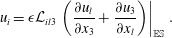 $$\begin{eqnarray}u_{i}=\unicode[STIX]{x1D716}{\mathcal{L}}_{il3}\left.\left(\frac{\unicode[STIX]{x2202}u_{l}}{\unicode[STIX]{x2202}x_{3}}+\frac{\unicode[STIX]{x2202}u_{3}}{\unicode[STIX]{x2202}x_{l}}\right)\right|_{\mathbb{ES}}.\end{eqnarray}$$
Equation (2.27) is valid for planar surfaces parallel to the plane
 $x_{3}=0$
. For such surfaces,
 ${\mathcal{L}}_{3l3}$
is zero, owing to the antisymmetry of the microscopic non-diagonal components
 $\unicode[STIX]{x1D613}_{3l3}$
in (2.21) (see § 3). Hence, according to (2.27), the wall-normal velocity,
 $u_{3}$
, is zero on
 $\mathbb{ES}$
. For an arbitrarily shaped surface, (2.27) may be generalized as
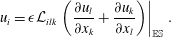 $$\begin{eqnarray}u_{i}=\unicode[STIX]{x1D716}{\mathcal{L}}_{ilk}\left.\left(\frac{\unicode[STIX]{x2202}u_{l}}{\unicode[STIX]{x2202}x_{k}}+\frac{\unicode[STIX]{x2202}u_{k}}{\unicode[STIX]{x2202}x_{l}}\right)\right|_{\mathbb{ES}}.\end{eqnarray}$$
In (2.28), the components of the slip tensor
 ${\mathcal{L}}_{ilk}$
are obtained by applying to their counterparts in (2.27) the transformation mapping the Cartesian coordinates onto the local system of reference of the surface under consideration. This implies that we implicitly assume that the unit cell remains a rectangular cuboid in the case of curved surfaces. This is a good approximation if the separation of scales is sufficiently large, i.e. the radius of curvature of the surface at the microscale is negligible with respect to its macroscopic counterpart. With the notation used in (2.28), it is not obvious that the wall-normal velocity remains zero on a curved surface; this will however be shown to be the case in appendix A.
Equation (2.28) represents the general tensorial form of the Navier slip condition (Navier Reference Navier1823), with the classical slip length changed into the slip tensor
 ${\mathcal{L}}_{ijk}$
. The procedure used to determine this tensor is the natural extension to three dimensions of the approach initiated by Jiménez Bolaños & Vernescu (Reference Jiménez Bolaños and Vernescu2017). It must be observed that when the surface is smooth, the no-slip condition is recovered with (2.28) by considering the limit
 $\unicode[STIX]{x1D716}\rightarrow 0$
. Thus, (2.28) is a generic boundary condition that applies to any surface exhibiting small roughness (Luchini Reference Luchini2013), the amplitude of which is measured by
 $\unicode[STIX]{x1D716}$
.
3 Solution of the microscopic problem for a hexagonal lattice of cylinders
The slip tensor
 ${\mathcal{L}}_{ijk}$
is the crucial ingredient for the applicability of (2.28). Physically, it represents the macroscopic counterpart of the microscopic structure and contains information on the geometry of the protrusions and their distribution. As already observed, it is defined as the volume average of the tensor obtained by solving the microscopic problem (2.21). Here we analyse the values of this tensor’s components first microscopically and then from an effective point of view. Even though (2.21) involves in principle eight equations and eight unknowns (six values for
 $\unicode[STIX]{x1D613}_{il3}$
, two for
 $\unicode[STIX]{x1D609}_{l3}$
), it can be split into two uncoupled Stokes problems with a surface forcing on
 $\mathbb{T}$
, one for
 $(\unicode[STIX]{x1D613}_{i13},\unicode[STIX]{x1D609}_{13})$
and one for
 $(\unicode[STIX]{x1D613}_{i23},\unicode[STIX]{x1D609}_{23})$
. We refer to appendix B for details about the numerical resolution of this system. The sizes
 $l_{1}$
,
 $l_{2}$
and
 $l_{3}$
of the microscopic cell,
 $\mathbb{V}$
, are sketched in figure 1. When the geometry of the lattice is established,
 $l_{1}$
and
 $l_{2}$
are fixed, while
 $l_{3}$
is still a free parameter with the only constraint that it must be of the same order of magnitude as
 $l_{1}$
and
 $l_{2}$
, so that the ‘small roughness’ constraint (Luchini Reference Luchini2013) is satisfied. Assuming that each hexagon of the lattice has a side length equal to 1 (normalizing lengths with
 $l$
) implies that
 $l_{1}=3$
and
 $l_{2}=\sqrt{3}$
, as sketched in figure 1. By construction, the protrusions have a height
 ${\hat{h}}$
equal to
 $l$
(
 $h={\hat{h}}/l=1$
). The dimensional radius of the protrusions is denoted with
 $\hat{r}$
, and
 $r=\hat{r}/l$
.
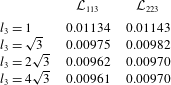
Components
 ${\mathcal{L}}_{ijk}$
of the volume-averaged slip tensor evaluated with different heights of the microscopic cell (
 $r=0.5751$
).
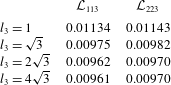
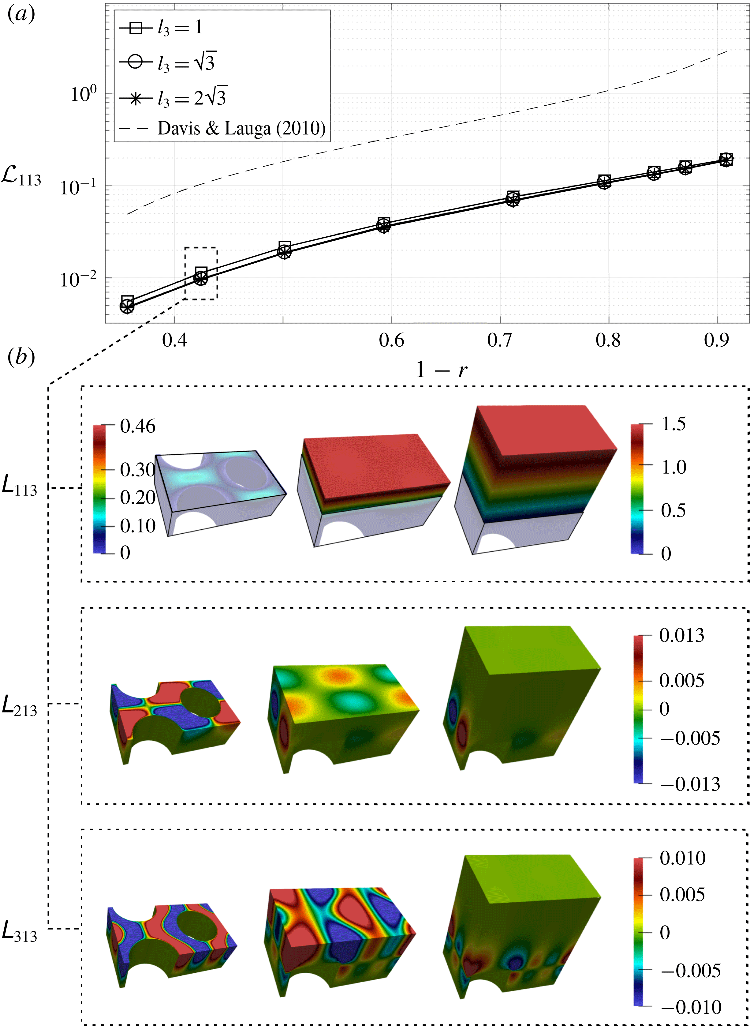
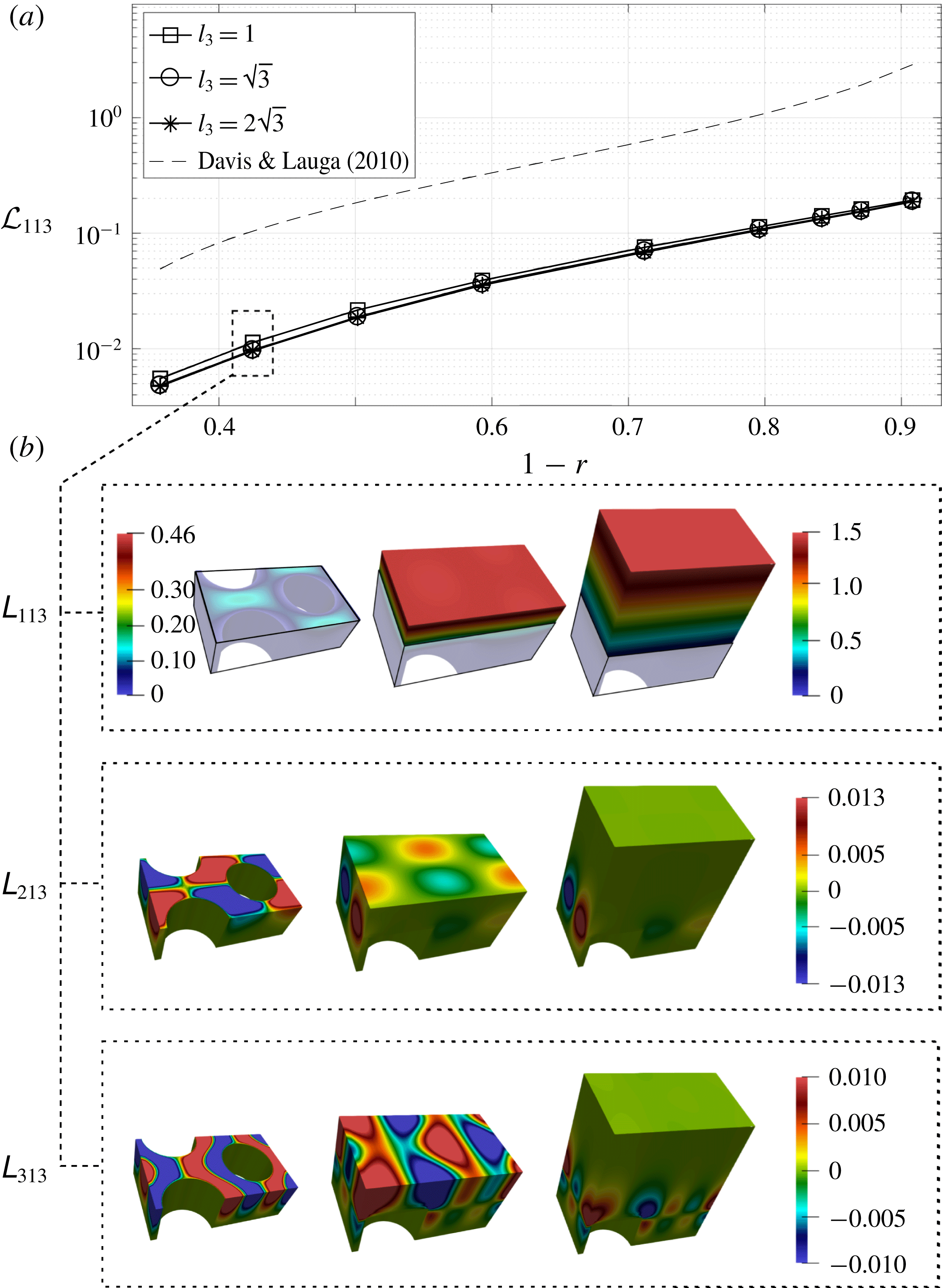
Figure 2 is representative of the microscopic behaviour of
 $\unicode[STIX]{x1D613}_{i13}$
(
 $\unicode[STIX]{x1D609}_{l3}$
is not shown because it does not play any role in the macroscopic equation since
 $\langle \unicode[STIX]{x1D609}_{l3}\rangle =0$
). The insets in figure 2 display the components of the vector
 $\unicode[STIX]{x1D613}_{i13}$
,
 $i=1,2,3$
, within
 $\mathbb{V}$
. Microscopically, the solution exhibits an analogous behaviour for each value of
 $l_{3}$
. A dominant component is found in the direction along which the flow is forced. The other components are antisymmetric with respect to
 $x_{2}=0$
(
 $\unicode[STIX]{x1D613}_{213}$
) or
 $x_{1}=0$
(
 $\unicode[STIX]{x1D613}_{313}$
). This implies that the corresponding components of the effective tensor are equal to zero. These symmetry properties are characteristic of orthotropic geometries, inherited from the cylindrical shape of the protrusions. In the same figure, the variation of
 ${\mathcal{L}}_{113}$
with the radius
 $r$
is described for several prescribed values of
 $l_{3}$
: increasing
 $l_{3}$
, the computed component of the slip tensor reaches an asymptotic value for each
 $r$
. For a given
 $l_{3}$
, the maximum slip is reached when the fluid-to-solid ratio within the unit cell is high, i.e. when the cylindrical protrusions become more slender. The same happens for
 ${\mathcal{L}}_{223}$
, the microscopic distribution of which is not shown since it can be deduced by symmetry because the selected hexagonal lattice exhibits
 $\mathbb{C}_{3}$
rotational symmetry. Table 1 details the typical behaviour of
 ${\mathcal{L}}_{ijk}$
when
 $l_{3}$
increases. The small differences that can be noticed between
 ${\mathcal{L}}_{113}$
and
 ${\mathcal{L}}_{223}$
are related to the anisotropy of the cuboid-shaped unit cell chosen to define the microscopic problem. For the sake of a qualitative comparison, it is interesting to confront the components of the slip tensor
 ${\mathcal{L}}_{ijk}$
found here with the results presented by Davis & Lauga (Reference Davis and Lauga2010), which refer to an ordered distribution of cylinders at a flat, no-shear gas–liquid interface corresponding to a Cassie–Baxter fluid–solid contact state (De Gennes, Brochart-Wyart & Quéré Reference De Gennes, Brochart-Wyart and Quéré2003). Clearly, this case, which corresponds to a ‘superhydrophobic’ behaviour, cannot be achieved with the Wenzel-like fluid–solid contact considered here. Hence the components of the slip tensor found by Davis & Lauga (Reference Davis and Lauga2010) are necessarily larger than those calculated here. However, figure 2 reveals an important analogy with their results: apart from a multiplicative constant, the dependency of
 ${\mathcal{L}}_{113}$
with respect to
 $r$
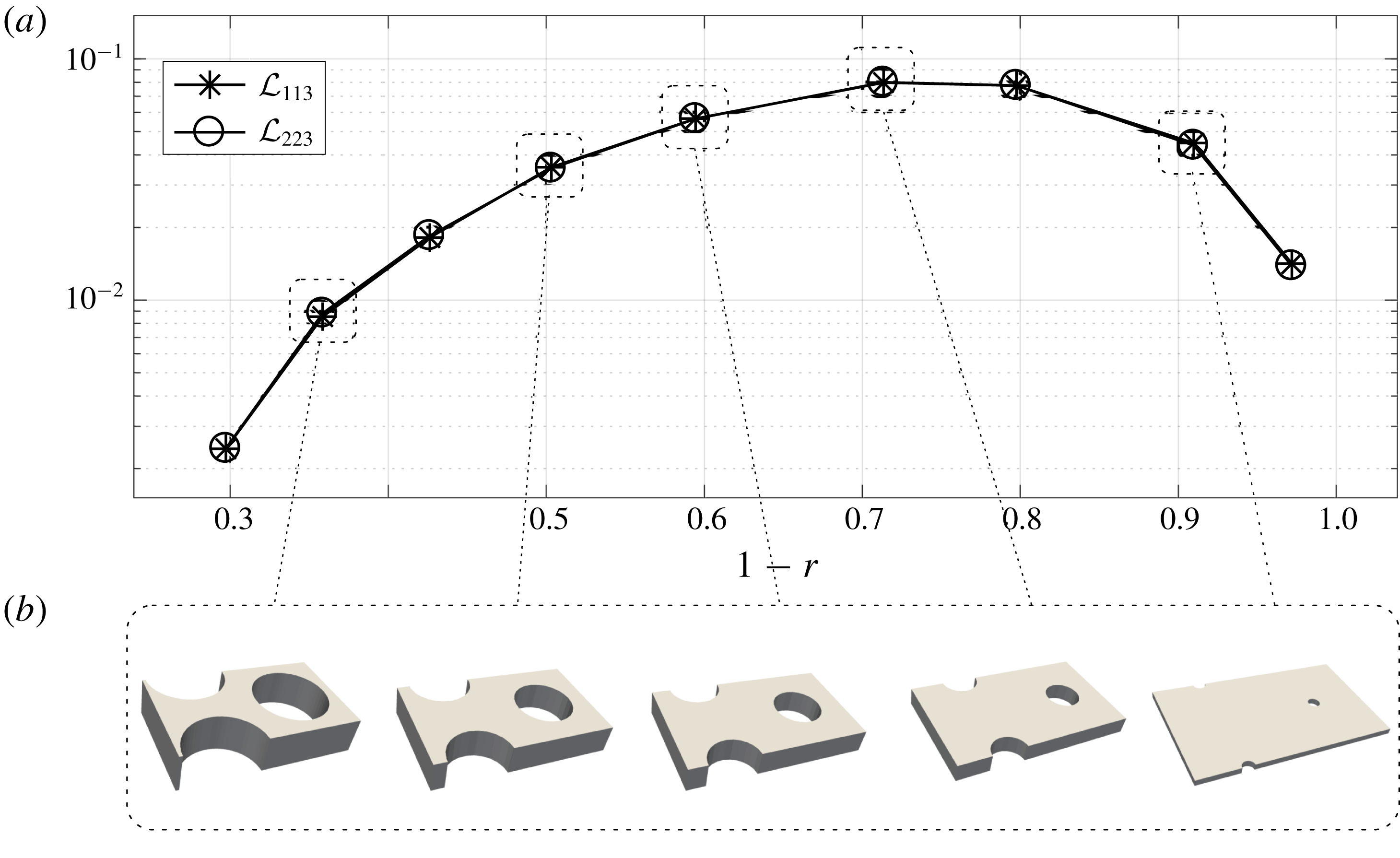
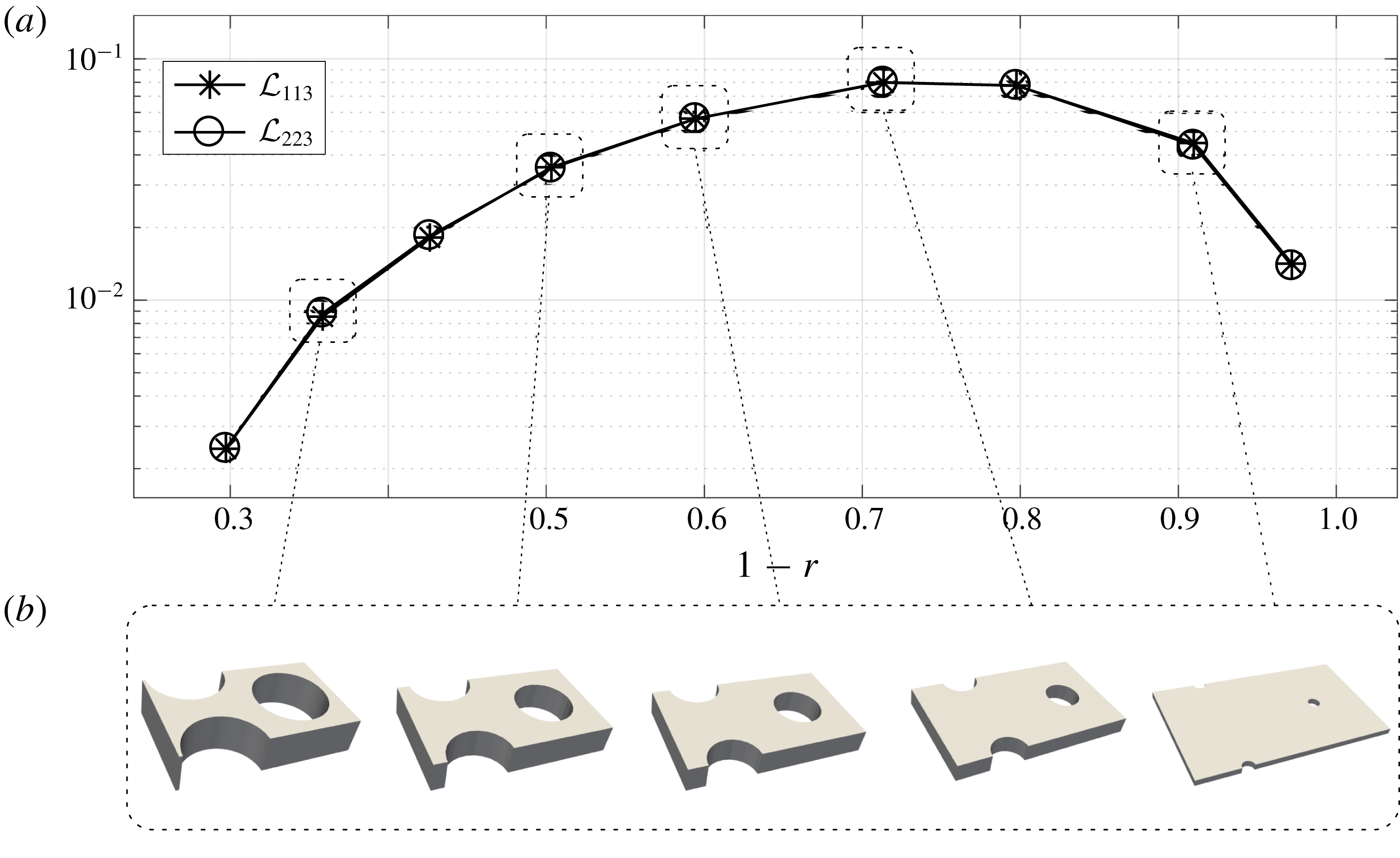
is similar in the two cases. Finally, it is of interest to show that the present homogenization approach, which provides a rigorous strategy to compute the microscopic slip tensors, is a flexible tool. Let us assume that for some reason, the design of the protrusions has to be modified, maintaining the geometrical constraint
 $h=r$
. This implies that we are considering cells such that
 $l_{3}=l_{3}(h(r))$
is an increasing function of
 $r$
. Computing the values of the slip tensor in this case yields the curve plotted in figure 3. This curve allows the value of
 $r$
(close to 0.2876 in this case) which maximizes
 ${\mathcal{L}}_{ijk}$
, and hence the modulus of the macroscopic slip velocity on the surface, to be readily selected. This can be of practical use to design surfaces in view of optimal drag reduction.
Variation of the slip tensor components with the fluid-to-solid ratio and cell height. (a) Variation of the volume-averaged component,
 ${\mathcal{L}}_{113}$
, with
 $r$
, for different cell heights. As
 $l_{3}$
is increased,
 ${\mathcal{L}}_{113}$
reaches an asymptotic value; the superhydrophobic results of Davis & Lauga (Reference Davis and Lauga2010) are also shown. (b) Microscopic components,
 $\unicode[STIX]{x1D613}_{i13}$
, for each
 $l_{3}$
when
 $r=0.5751$
and
 $h=1$
. In the image displaying
 $\unicode[STIX]{x1D613}_{113}$
, the scale on the left (respectively right) refers to the solutions for
 $l_{3}=1$
and
 $l_{3}=\sqrt{3}$
(respectively
 $l_{3}=2\sqrt{3}$
). As the microscopic solution shows, the off-diagonal component
 $\unicode[STIX]{x1D613}_{213}$
is antisymmetric, which results in a zero average once (2.23) is applied. Each value in (a) corresponds to the average over the shadowed region shown in the microscopic visualization of
 $\unicode[STIX]{x1D613}_{113}$
.
(a) Effective slip for protrusions designed in different ways. (b) Sample geometries for varying
 $r$
.
4 A rough sphere in a uniform stream
Condition (2.28) holds over arbitrary surfaces with small roughness, provided that the periodicity condition holds along
 $x_{1}$
and
 $x_{2}$
, so that the effective slip tensor can be computed for the associated microscopic geometry. In this section we define a test configuration which consists of the flow past a rough spherical particle (RSP). This configuration is used on the one hand to validate the homogenized model in the laminar regime, and on the other hand to discuss its validity in the turbulent regime. To validate (2.28), a fully three-dimensional case, such as the flow past a sphere, is of fundamental interest because the novelty of the model resides in the fact that it is valid for generically shaped surfaces. Moreover, rough spherical particles are involved in many flows of engineering or environmental relevance, from fluidized beds to hailstones showers to mention just two examples. As described later in this section, we carried out fully resolved DNS of the flow past a RSP. The computation and properties of the microscopic solution associated with the lattice built on the sphere have been already discussed in § 3, while the macroscopic solution for this particular configuration is presented in § 5.
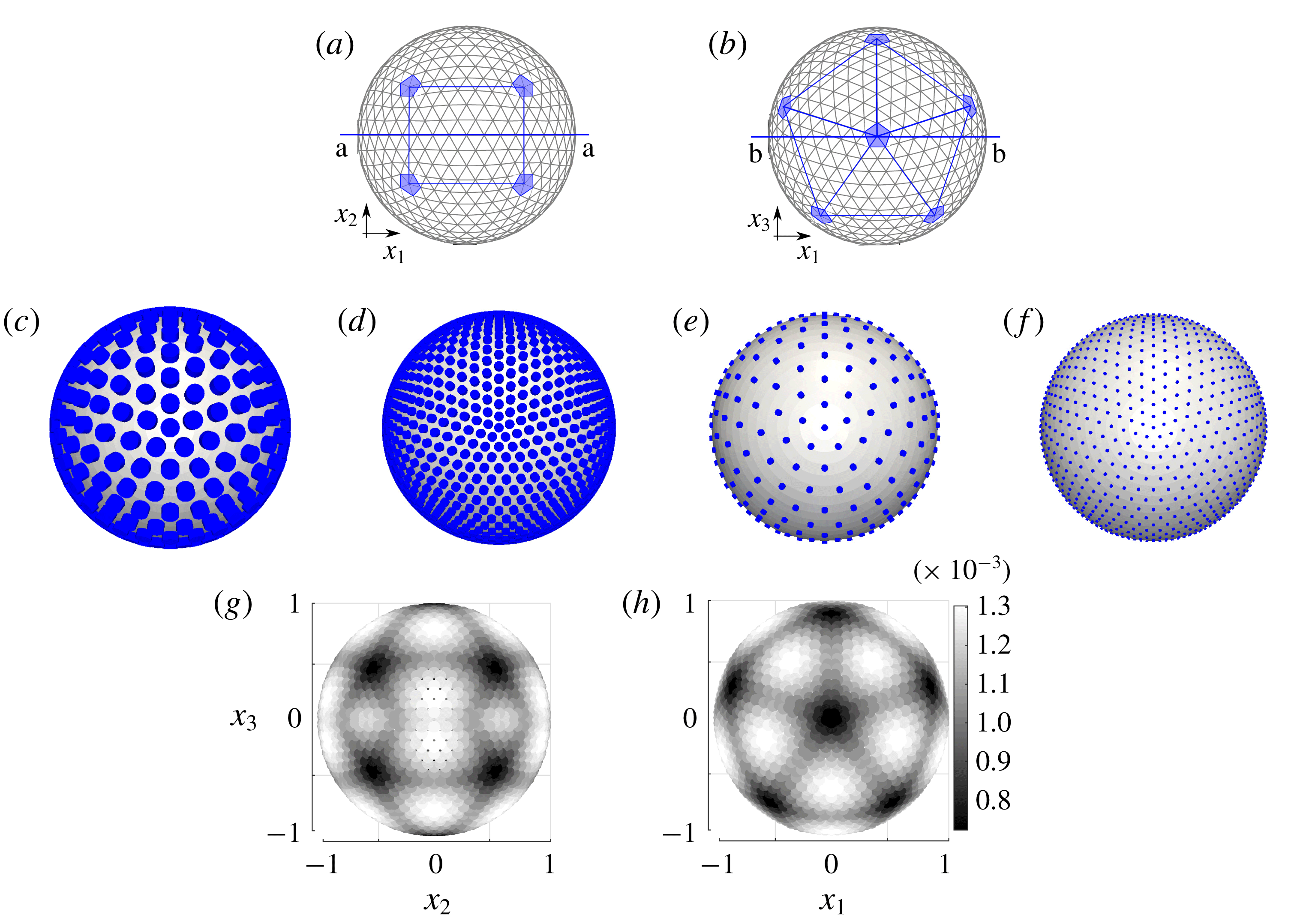
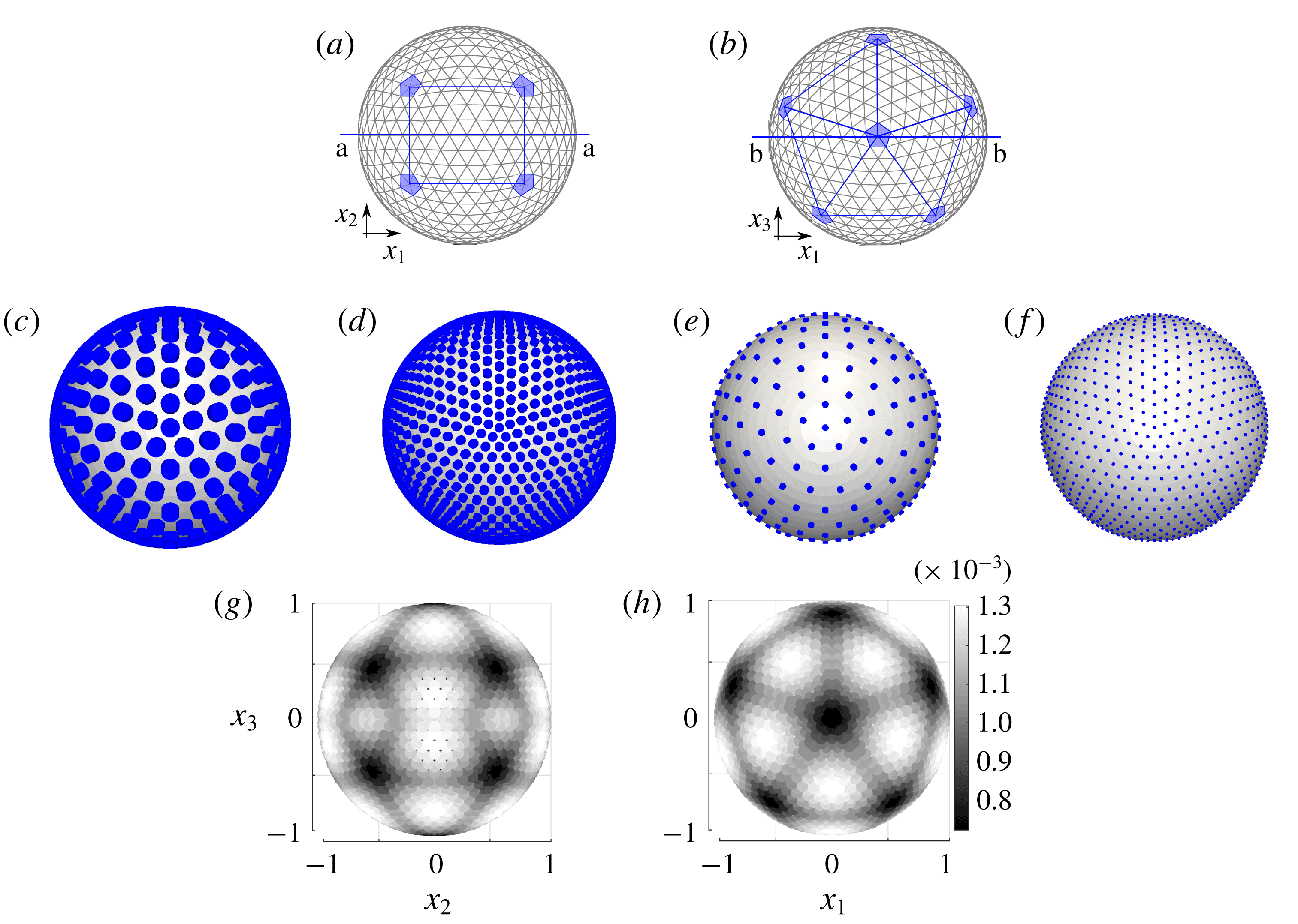
(a,b) Icosahedral discretization of a sphere (
 $\unicode[STIX]{x1D709}=8$
); front (a) and top (b) view. A protrusion is placed at each vertex of the icosahedron. (c–f) Examples of macroscopic spheres covered by cylindrical protrusions for the following values of the parameters:
 $\hat{r}/R^{inn}=0.5751\unicode[STIX]{x1D716}$
(c,d),
 $\hat{r}/R^{inn}=0.2023\unicode[STIX]{x1D716}$
(e,f), with
 $\unicode[STIX]{x1D709}=6$
(c,e) and
 $\unicode[STIX]{x1D709}=12$
(d,f). For the four cases shown,
 ${\hat{h}}/R^{inn}=\unicode[STIX]{x1D716}$
. (g,h) Distribution of the non-homogeneity in the coverage of the icosahedron surface for
 $\unicode[STIX]{x1D709}=12$
(front and top views, respectively). The grey scale indicates the area of each face of the icosahedron; this area decreases as the poles are approached.
4.1 Designing a rough sphere
The RSP is built by covering the sphere with a hexagonal lattice of cylinders (cf. figure 1). Unfortunately, neither this lattice, nor any other planar lattice, obtained through the periodic repetition of a single planar figure can cover a sphere, due to the fact that its curvature prevents the existence of a bijective mapping with a plane, able to preserve at the same time areas, lengths and angles. For this reason, we seek a distribution of protrusions which is as isotropic as possible and as close as possible to that introduced in figure 1, so that the global dynamics of the RSP may be compared with that of a smooth spherical particle (SSP). A quasi-isotropic distribution is achieved by discretizing the sphere as a quasi-regular icosahedron. This is a polyhedron characterized by twelve special points, the poles, that divide the sphere into fifteen portions (ten of them triangular and the other five rectangular), and by a frequency,
 $\unicode[STIX]{x1D709}$
, representing the number of sides between two consecutive poles belonging to a triangular portion (see figure 4
a,b).
The residual non-homogeneity of the distribution at the surface of the icosahedron arises from the presence of the twelve poles (figure 4
g,h). Despite this imperfect distribution, it will be shown later that the homogenization approach may be applied successfully. Different examples of coatings are shown in the central row of figure 4, for different values of
 $\unicode[STIX]{x1D709}$
,
 $\hat{r}/L$
and
 ${\hat{h}}/L$
. These parameters univocally define the coating of the sphere. The macroscopic scale
 $L$
is set to
 $R^{inn}$
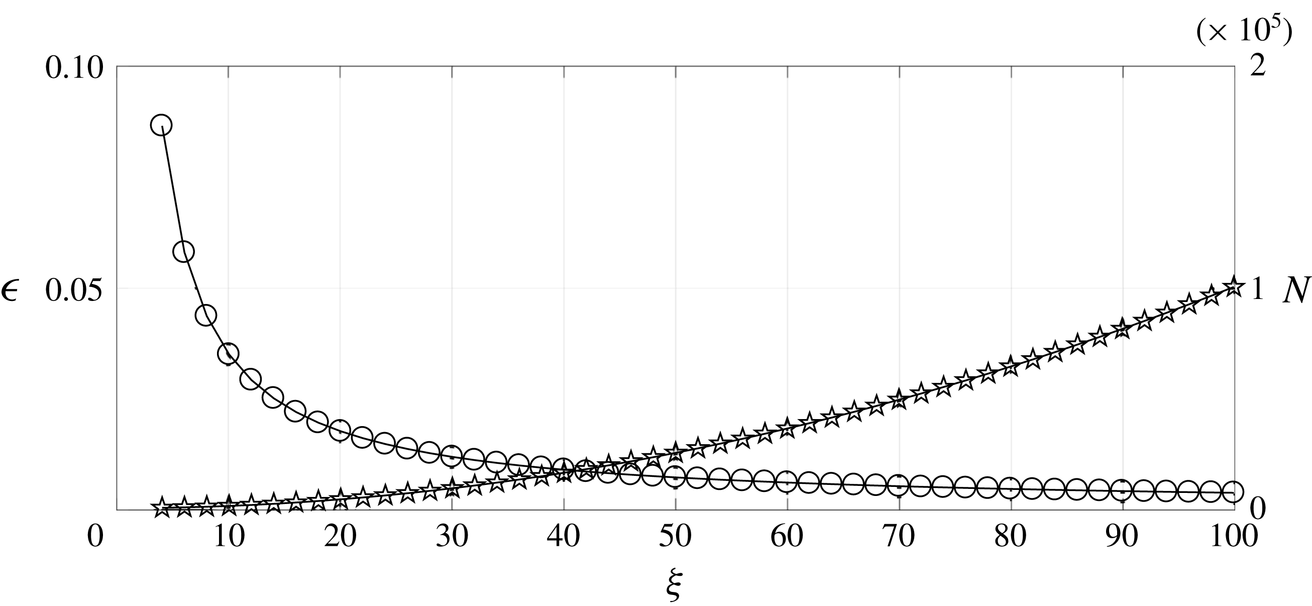
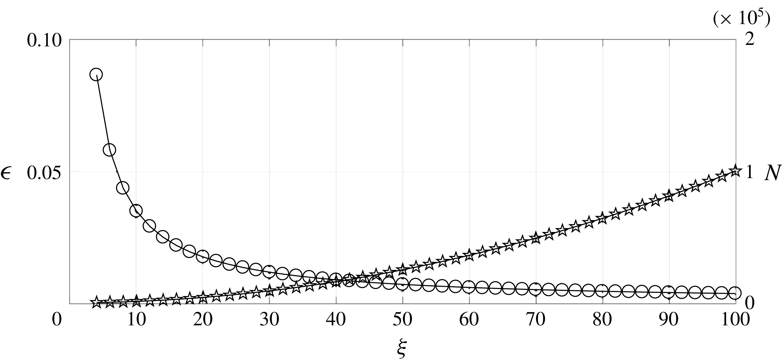
, the radius of the smooth sphere at the surface of which the protrusions are placed. Figure 5 shows how the parameter
 $\unicode[STIX]{x1D716}=l/L={\hat{h}}/R^{inn}$
and the total number of protrusions,
 $N$
, depend on
 $\unicode[STIX]{x1D709}$
. A small decrease in
 $\unicode[STIX]{x1D716}$
is seen to correspond to a large increase in
 $\unicode[STIX]{x1D709}$
, hence in the number of protrusions. This means that performing a direct numerical simulation of the RSP with a small
 $\unicode[STIX]{x1D716}$
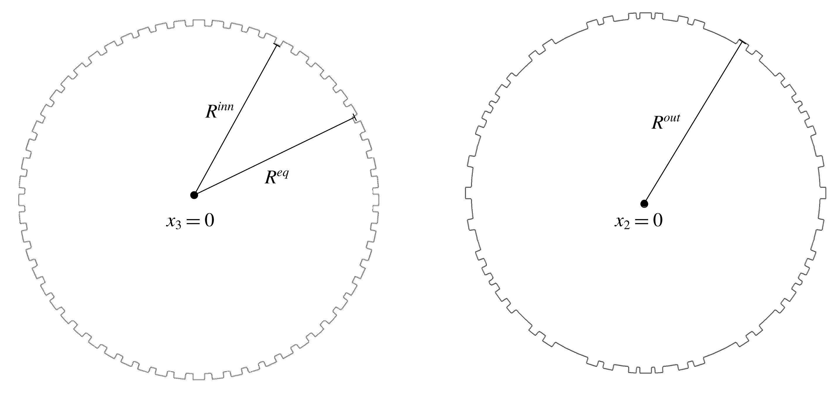
(i.e. in the limit of homogeneous roughness) would imply a large computational cost. Clearly, the macroscopic analogy becomes very useful in this limit. In this analogy, two related but distinct objects play a role. The first of them is the RSP, characterized by
 $R^{inn}$
and
 $R^{out}=R^{inn}(1+\unicode[STIX]{x1D716})$
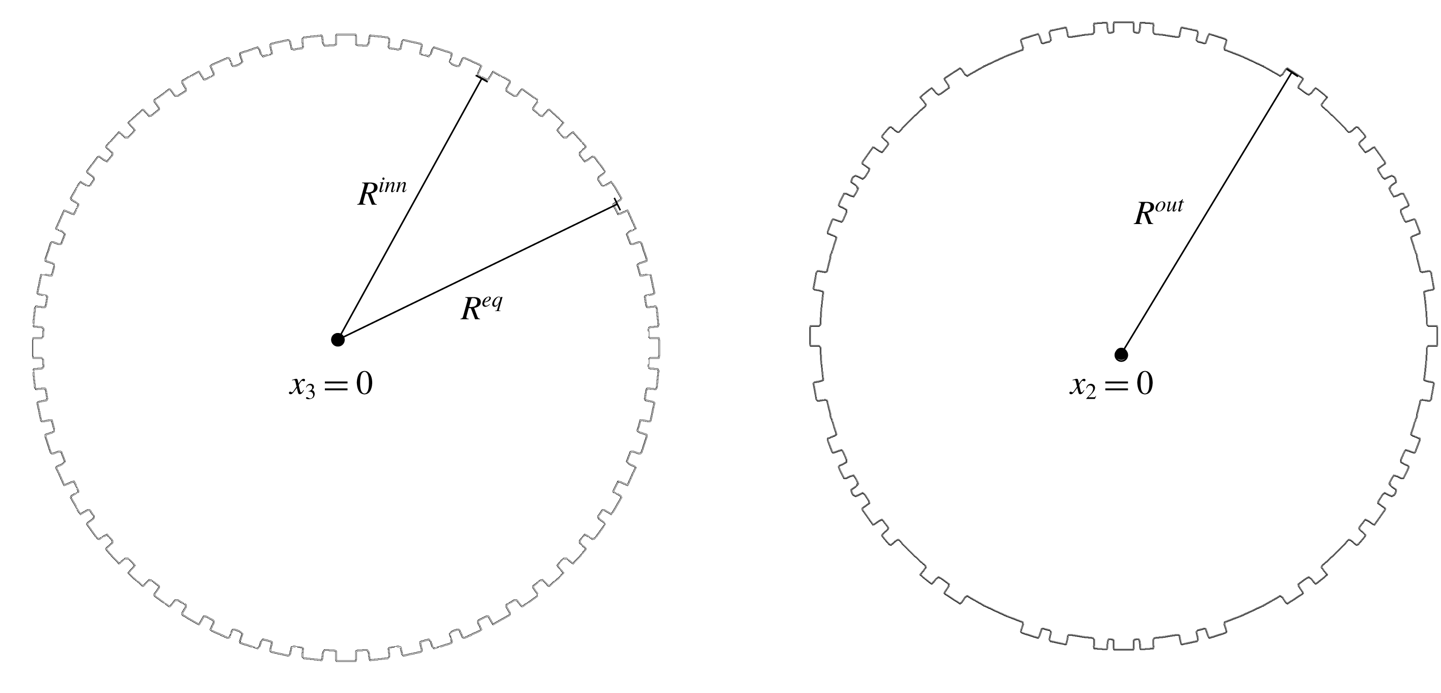
, the radius of the outer spherical particle defined as the smooth sphere tangent to the crests of the roughness elements. The second is the equivalent spherical particle (ESP), the characteristic radius of which is
 $R^{eq}$
(see figure 6). The ESP has the same macroscopic physical properties as the corresponding RSP and is expected to behave in the same manner, provided that the condition (2.28) is imposed over its surface. The equivalent radius depends in principle on the shape of the protrusions (in the case of cylinders defined by
 $\hat{r}/R^{inn}$
and
 ${\hat{h}}/R^{inn}$
) and on the parameter
 $\unicode[STIX]{x1D709}$
. One expects
 $R^{eq}$
to lie in between
 $R^{inn}$
and
 $R^{out}$
, which will be confirmed later on a selected example.
Variation of
 $\unicode[STIX]{x1D716}$
(circles, scale on the left vertical axis) and the number of protrusions
 $N$
(stars, scale on the right vertical axis) with respect to the frequency
 $\unicode[STIX]{x1D709}$
of the icosahedron.
Cut of the simulated RSP across two orthogonal planes. The non-homogeneity in the distribution of the protrusions can be observed;
 $R^{inn}$
,
 $R^{eq}$
and
 $R^{out}$
denote the inner, equivalent and outer radius, respectively.
4.2 The reference DNS
To perform direct numerical simulations of a uniform flow past the RSP we have just designed, we employ the OpenFOAM software with a computational domain of rectangular cuboid shape of size
 $200\times 80\times 80$
, in
 $R^{inn}$
-units. A zero velocity gradient boundary condition is imposed at the outlet (Versteeg & Malalasekera Reference Versteeg and Malalasekera2007). Thanks to this domain size, the physical quantities relevant to the sphere-induced disturbance are not influenced by the outer boundaries in the considered range of Reynolds number (see appendix B). A constant inlet velocity
 $(1,0,0)$
is imposed at
 $x_{1}=0$
, while symmetry conditions are imposed on the
 $(x_{1},x_{2})$
and
 $(x_{1},x_{3})$
outer planes, to simulate an unbounded domain.
Before comparing macroscopic simulations and DNS results, we analyse the latter in the case of a rough sphere with
 $Re^{out}=100$
(based on the sphere inner diameter and the incoming, uniform speed),
 $\hat{r}/R^{inn}=0.017$
,
 ${\hat{h}}/R^{inn}=\unicode[STIX]{x1D716}=0.029$
and
 $\unicode[STIX]{x1D709}=12$
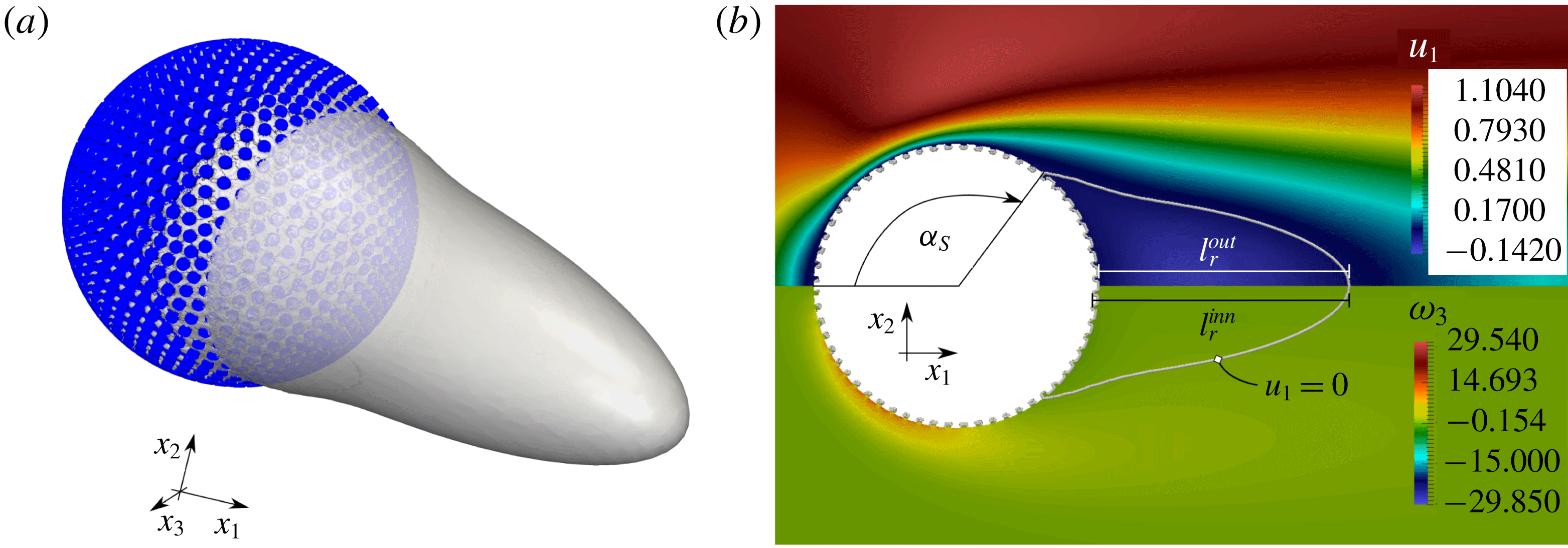
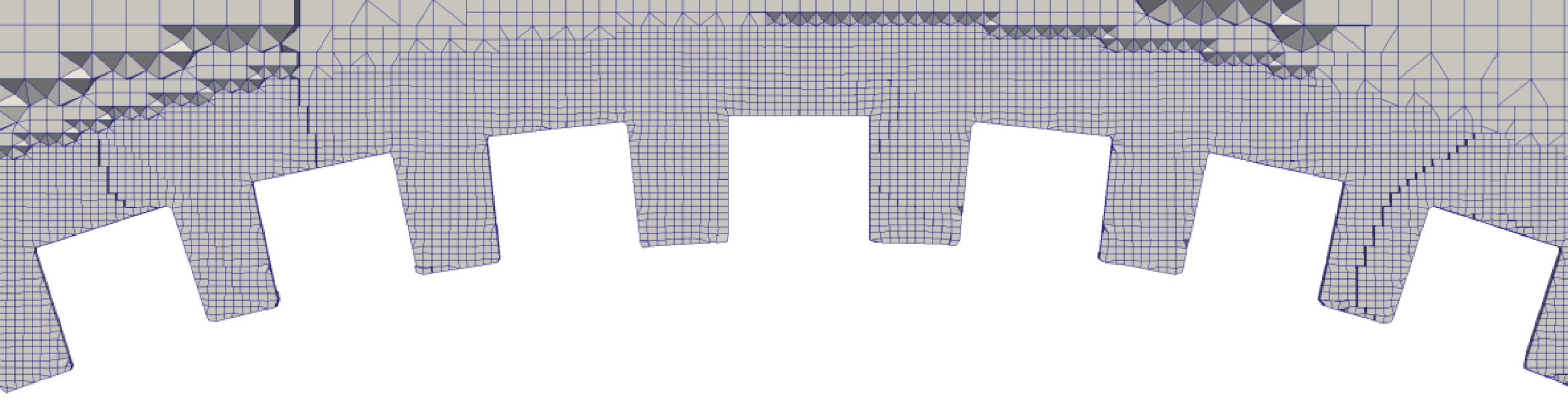
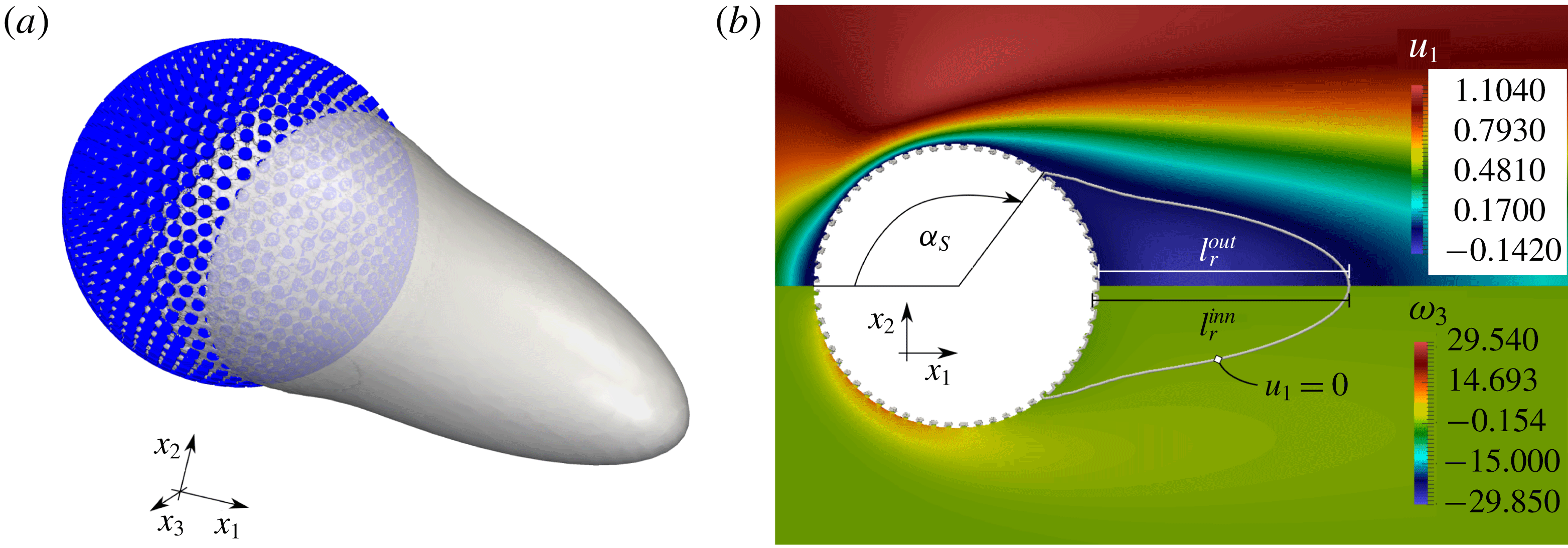
(a zoom of the grid used to discretize the flow close to the sphere surface is provided in figure 17). Figure 7 shows the geometry of the corresponding sphere surface, together with the streamwise velocity iso-surface
 $u_{1}=0$
(a). In (b), the iso-contours of
 $u_{1}$
and
 $\unicode[STIX]{x1D714}_{3}$
are represented, together with the separation angle,
 $\unicode[STIX]{x1D6FC}_{S}$
, and the recirculation lengths
 $l_{r}^{inn}$
and
 $l_{r}^{out}$
measured with respect to the inner and outer sphere radii, respectively. Figure 8 displays some iso-contours of the two velocity components
 $u_{1}$
and
 $u_{3}$
in the cross-sectional plane
 $x_{2}=0$
, in the case of a SSP with
 $R=1$
(red online) and
 $R=R^{out}/R^{inn}$
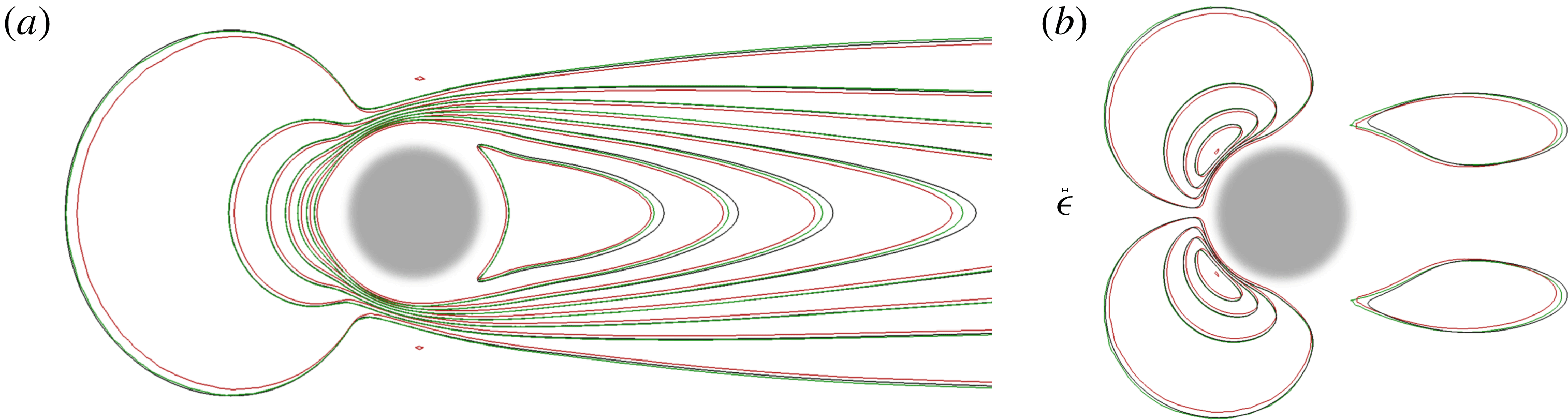
(green online), and the actual RSP (black). Differences between the three fields are of order
 $\unicode[STIX]{x1D716}$
, as predicted by Amirat et al. (Reference Amirat, Bresch, Lemoine and Simon2001). While the fields computed for the case of the RSP and the SSP with
 $R=R^{out}/R^{inn}$
are very similar in the region close to the sphere, more significant changes arising from the presence of the rough layer can be observed in the wake.
Several characteristics of the flow past a SSP and a RSP at
 $Re^{out}=100$
(the fluid density, upstream velocity and sphere inner radius are set to unity). The drag force,
 $F_{D}$
, is split into viscous,
 $F_{V}$
, and pressure,
 $F_{P}$
, components. The separation angle and recirculation length are defined in figure 7. The value of
 $\unicode[STIX]{x1D6FC}_{S}$
for the RSP shown in this table is a macroscopically averaged value which does not reflect the complex pointwise behaviour of the flow within the rough layer.

Flow past a RSP. (a) Iso-surface corresponding to
 $u_{1}=0$
(in grey). (b) Iso-contours of
 $u_{1}$
(top) and the third (azimuthal) component of the vorticity field,
 $\unicode[STIX]{x1D714}_{3}$
, (bottom) represented with colours. The thin grey line corresponds to the iso-contour
 $u_{1}=0$
. The recirculation length
 $l_{r}^{inn}$
(respectively
 $l_{r}^{out}$
) is defined with respect to the RSP inner (respectively outer) radius. The separation angle
 $\unicode[STIX]{x1D6FC}_{S}$
is measured clockwise, using the locally averaged fields calculated from the DNS, in the way explained in appendix B (§ B.4).
Iso-contours of
 $u_{1}$
(a) and
 $u_{3}$
(b) at
 $x_{2}=0$
(
 $u_{2}=0$
in this plane). Values of the
 $u_{1}$
(respectively
 $u_{3}$
) velocity component in the left (right) frame are equally spaced from
 $-0.132$
to
 $+1.105$
(respectively, from
 $-0.475$
to 0.475). The red and green (online) contours correspond to a SSP with a no-slip condition at
 $R=1$
and
 $R=R^{out}/R^{inn}$
, respectively, and the black lines to a RSP with
 $\hat{r}/R^{inn}=0.017$
,
 ${\hat{h}}/R^{inn}=0.029$
and
 $\unicode[STIX]{x1D709}=12$
. The reference size
 $\unicode[STIX]{x1D716}$
is shown to scale at the centre of the figure.
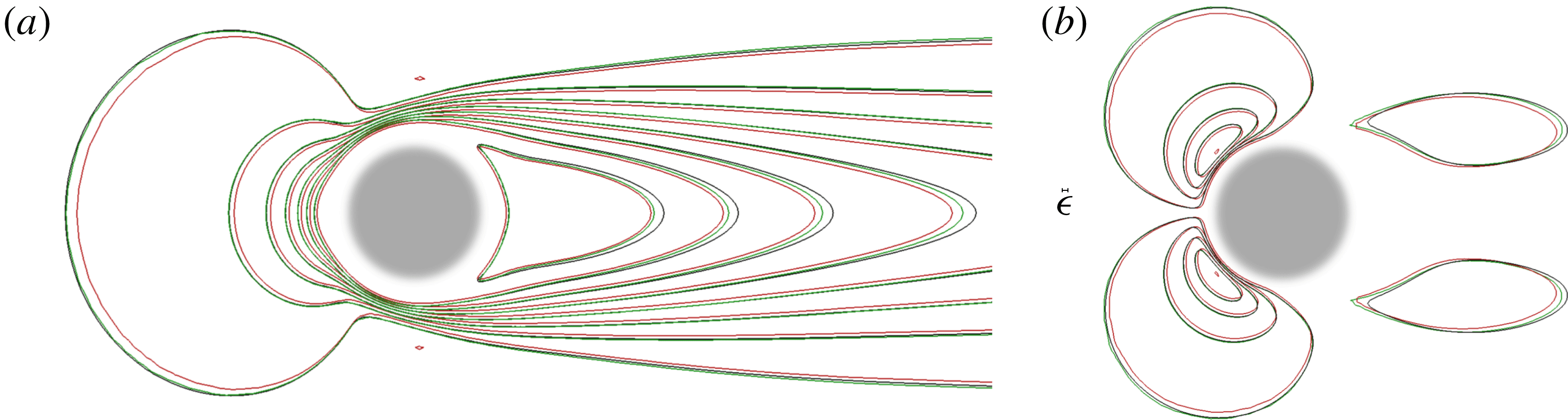
Table 2 reports the values of several quantities characterizing the flow past the sphere, especially the normalized drag force,
 $F_{D}$
, split into its viscous,
 $F_{V}$
, and pressure,
 $F_{P}$
, components. As the comparison with the SSP reveals, introducing the rough surface significantly increases the pressure drag (by nearly 30 %) and decreases its viscous counterpart (by 19 %). The changes in the total drag force are smaller due to the compensation between the variations of its two components. Note that, due to the weakly anisotropic distribution of the protrusions, the
 $x_{2}$
- and
 $x_{3}$
-components of the force acting on the RSP (not shown) are not strictly zero. However the corresponding values are very small and rapidly tend to zero as
 $\unicode[STIX]{x1D709}$
increases. Values of
 $\unicode[STIX]{x1D6FC}_{S}$
and
 $l_{r}^{out}$
given in the table indicate that the rough surface slightly delays separation and increases the recirculation length.
5 The macroscopic model: pros and cons
In this section, we apply the condition (2.28) on the equivalent fluid–solid surface to study the dynamics of the flow past the RSP described in the previous section. Our overall objective is to discuss and compare the results obtained through the pointwise description previously presented (i.e. the full DNS approach) with those provided by the macroscopic approach, in order to assess the applicability and accuracy of the homogenization framework. We first validate the boundary condition (2.28) in a laminar case. Then we consider a turbulent situation, in order to better identify its capabilities and shortcomings, by inspecting both the mean flow and the fluctuating field.
5.1 Laminar regime
Comparison of the streamwise velocity component,
 $u_{1}$
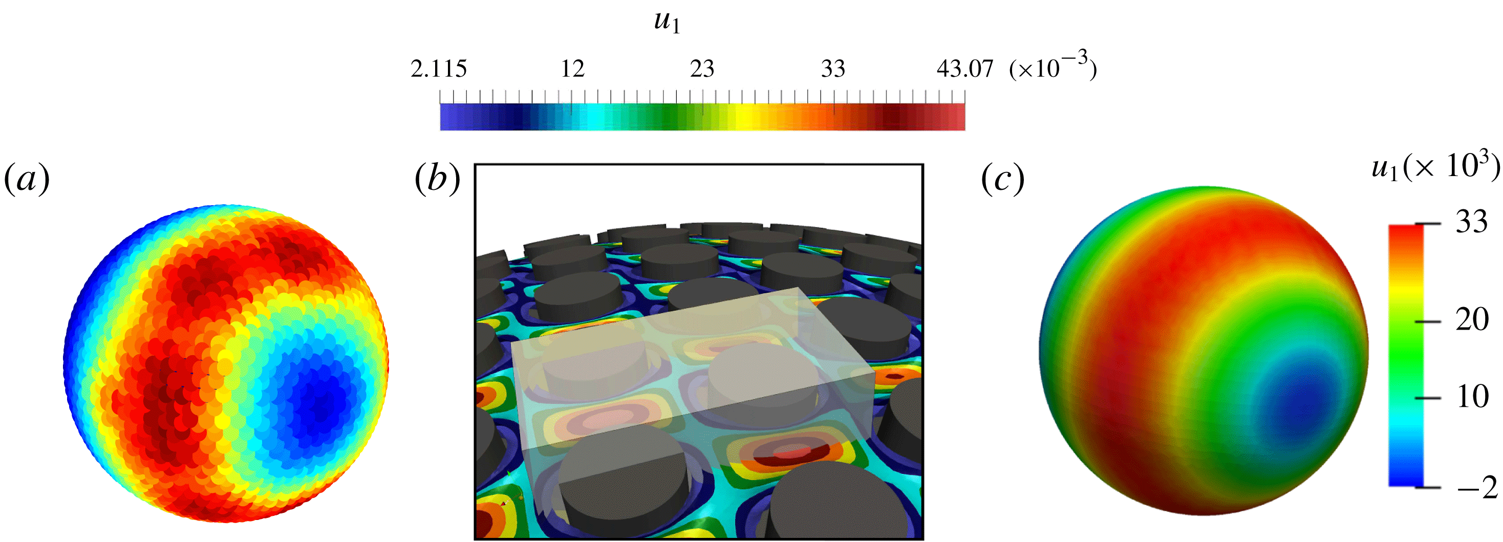
, on the sphere, computed with the macroscopic model (2.28) (c), and extracted from the reference DNS (a). The procedure used to pass from one approach to the other is detailed in the text. (b) The microscopic cell,
 $\mathbb{V}$
, (in grey), with the microscopic distribution of the
 $u_{1}$
iso-contours on a surface located slightly above
 $R=1$
.
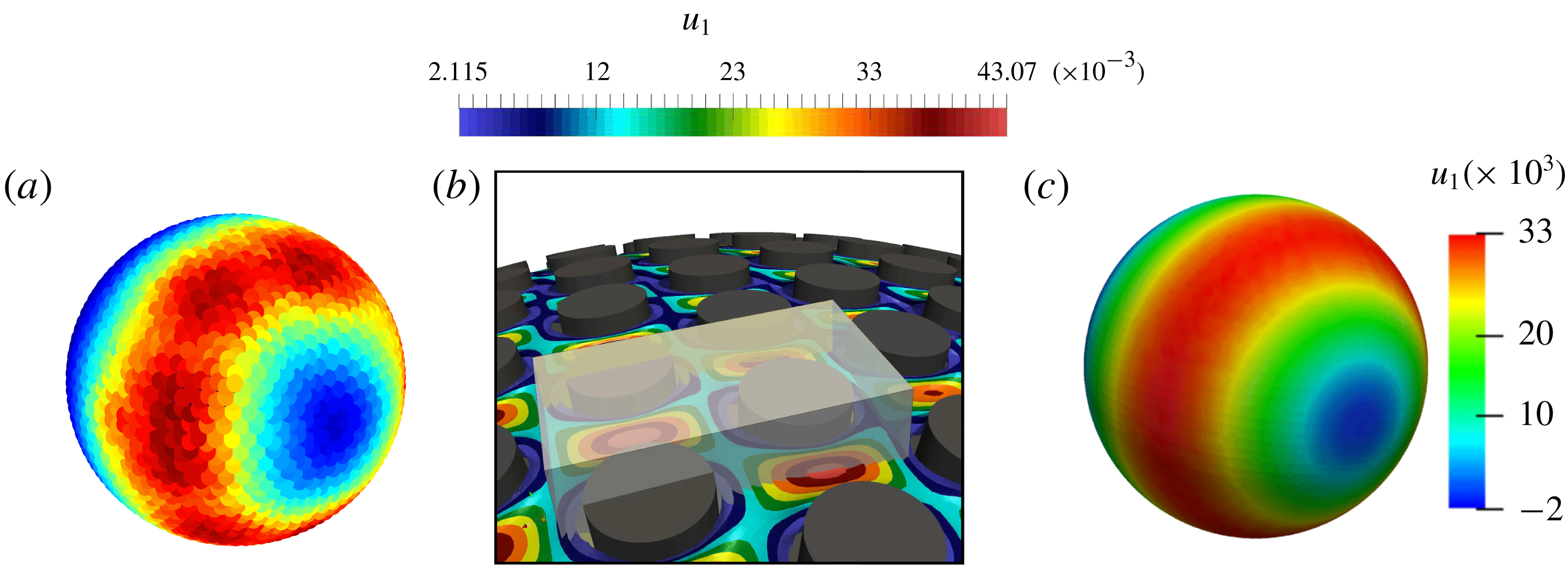
In § 4, the flow dynamics past the RSP was analysed microscopically using a complete DNS. To make the comparison between these results and those obtained with the ESP, we make use of the macroscopic analogy briefly mentioned at the end of § 4.1. To establish a one-to-one link between the macroscopic fields and those resolved at each scale in the DNS, it is sufficient to divide the rough layer in the latter into microscopic cells such as the transparent one shown in figure 9(b) and, for each field, calculate the average defined in (2.23). Each microscopic elementary cell corresponds to a macroscopic point on the ESP surface, identified by the centre of the cell’s face belonging to the sphere. Once the averaged fields have been extracted from the DNS, comparisons can be performed within two different orthogonal half-planes intersecting the sphere (e.g. those denoted as aa and bb in figure 4). Condition (2.28) is imposed at either
 $R=1$
or
 $R=R^{out}/R^{inn}=1+\unicode[STIX]{x1D716}$
, and we find the results to be indistinguishable to graphical accuracy. In the situation to be described below, the values of the relevant slip components are
 ${\mathcal{L}}_{113}=0.00975$
and
 ${\mathcal{L}}_{223}=0.00982$
. These values were computed as described in appendix B, using a microscopic cell with
 $\hat{l}_{3}=\sqrt{3}l$
.
A first qualitative comparison of the prediction provided by the two approaches for the main (streamwise) component of the velocity over the sphere may be inferred from figure 9(a,b).
In figure 9(a), one may notice a weak angular inhomogeneity in the
 $u_{1}$
-distribution, due to the non-homogeneity of the lattice covering the RSP. This inhomogeneity does not happen with the equivalent model in figure 9(c), since we assumed a perfectly periodic lattice to carry out the microscopic computations, which yields constant components
 ${\mathcal{L}}_{ijk}$
in the local reference frame of the sphere.
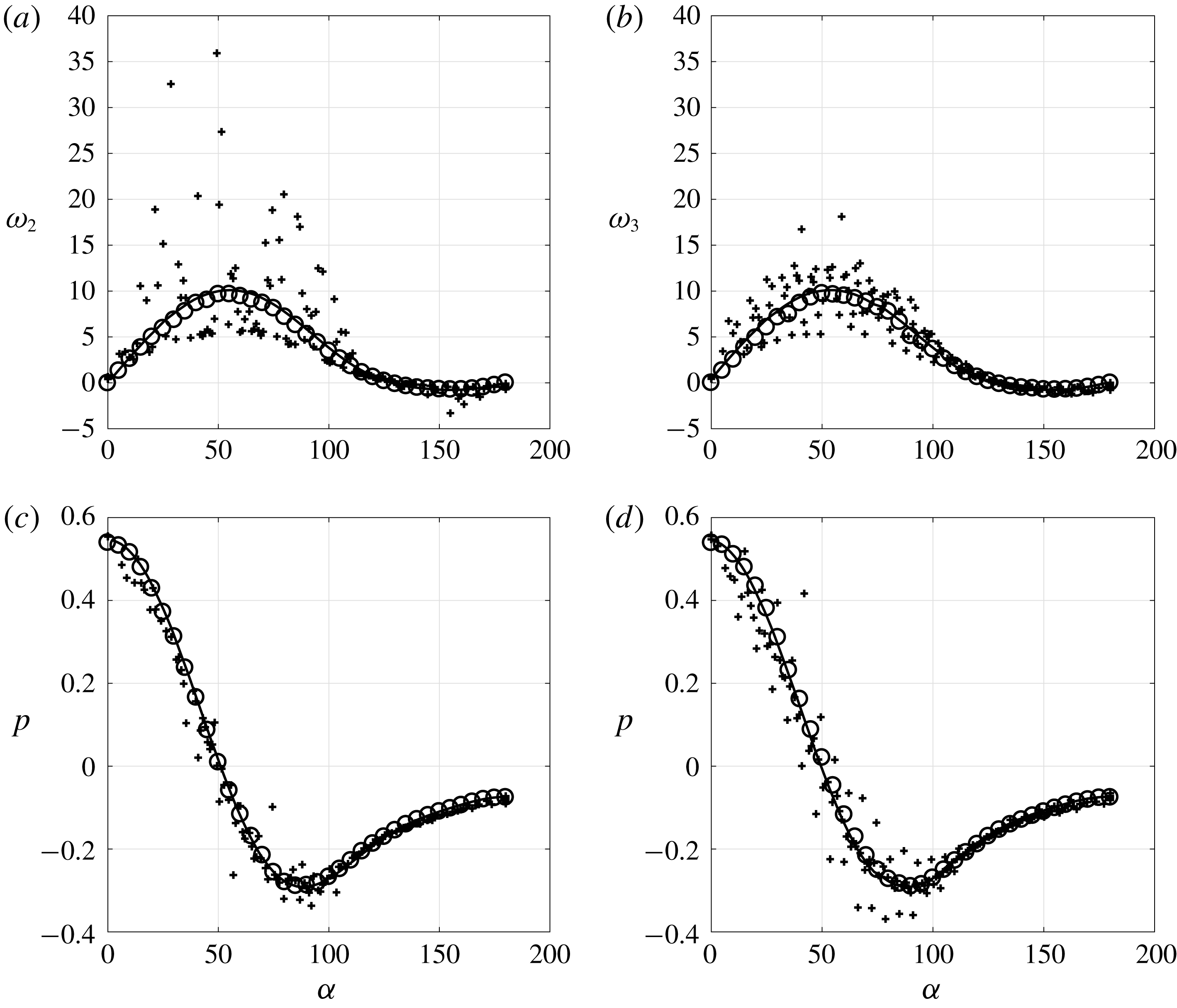
Surface distribution of the non-zero components of the surface vorticity,
 $\unicode[STIX]{x1D714}_{j}$
, and pressure,
 $p$
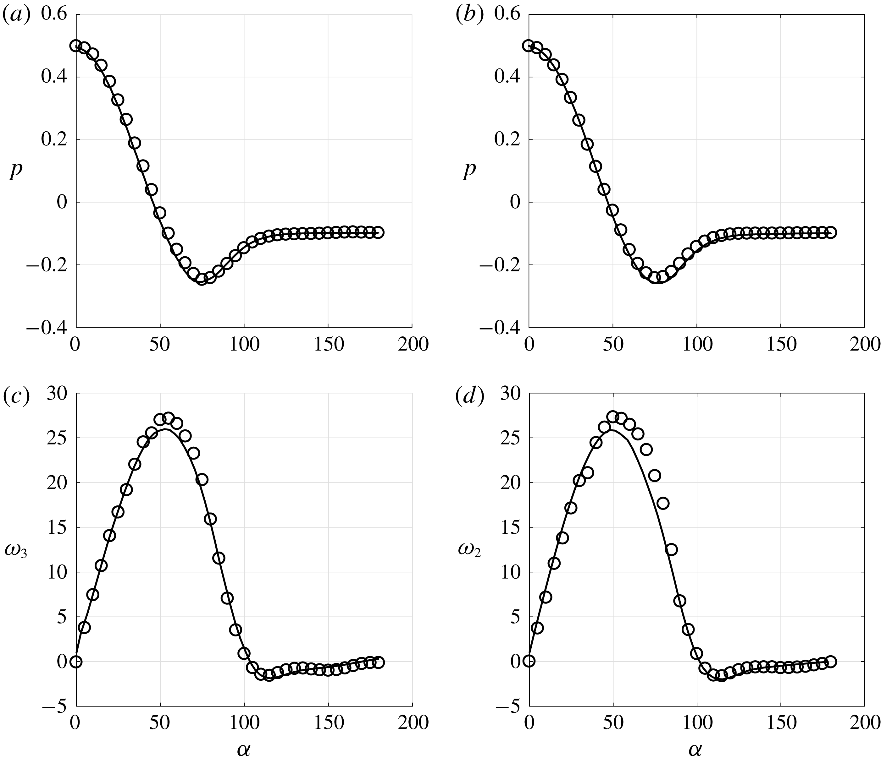
, along aa (a,c) and bb (b,d). Open circles: results extracted from the DNS upon averaging over the near-wall unit cell;
 $+$
symbols: pointwise DNS results; solid line: solution computed using (2.28) on the ESP.
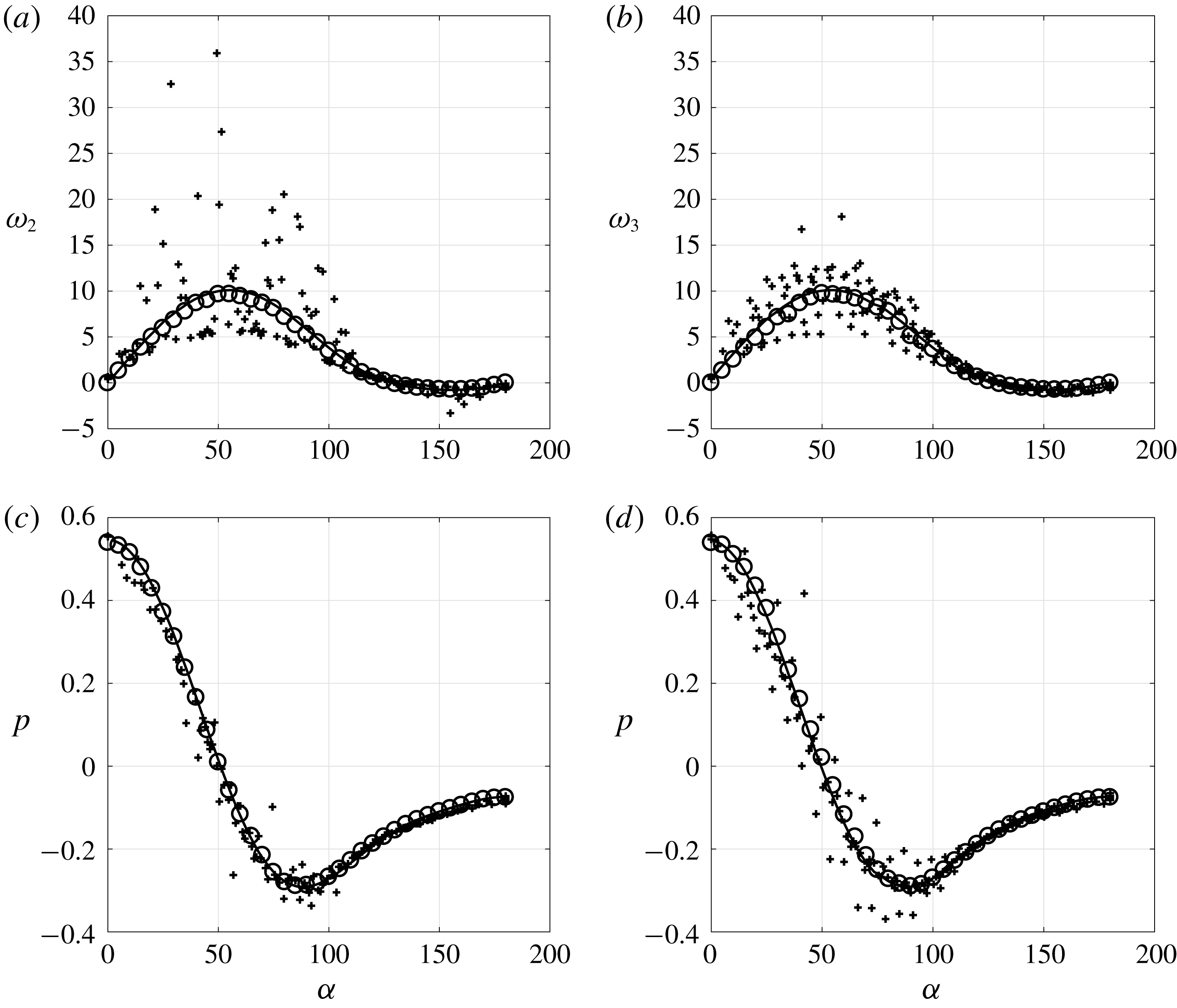
Figure 10 shows the distributions of the surface vorticity and pressure in the cross-sectional planes corresponding to the lines aa and bb in figure 4. A good agreement between the prediction based on condition (2.28) and the locally averaged distribution extracted from the DNS is observed. For completeness, the pointwise DNS results at
 $R=R^{out}/R^{inn}$
, in which no local averaging over the near-wall unit cells has been performed, are also shown. The oscillations displayed by these results are directly related to the presence of the roughness. They are of large amplitude, especially in the surface vorticity which has a direct link to the wall shear stress, and may reach local values 2 to 4 times larger than the maximum of their locally averaged counterpart. Given these strong oscillations, it is remarkable that the generalized Navier condition yields solutions which agree so well with the locally averaged DNS results.
Global quantities characterizing the flow past the sphere, evaluated with the macroscopic approach described in § B.4 (the value of
 $l_{r}$
with the asterisk is computed by considering the average between
 $l_{r}^{inn}$
and
 $l_{r}^{out}$
; in the macroscopic framework, deviations of
 $O(\unicode[STIX]{x1D716})$
from this value are allowed).

Table 3 summarizes some flow characteristics obtained using the DNS and the macroscopic model. The values in the first row of tables 2 and 3 refer to the same simulation. The two series of values for the force are different because they are computed using the pointwise approach in the former case, while the locally averaged fields are used in the latter (see § B.4 in appendix B). The presence of large oscillations in figure 10 explains why
 $F_{P}$
and
 $F_{V}$
differ in the two cases, whereas the two values of
 $F_{D}=F_{P}+F_{V}$
agree to within 5 %. From a global point of view, the model is again seen to approximate the locally averaged DNS results well, as differences between the various sets of normalized results are all less than
 $\unicode[STIX]{x1D716}$
. The results of two distinct simulations carried out past the ESP are also included in table 3; they help to appreciate the effect of the exact definition of the sphere radius (
 $R=1$
or
 $R=R^{out}/R^{inn}$
) where (2.28) is imposed. The differences obtained by imposing the ESP radius either at
 $R=1$
or at
 $R=R^{out}/R^{inn}$
are very small and nothing can be concluded regarding the ‘exact’ position of the equivalent surface. This is in agreement with the level of accuracy of the theory: since we are computing an
 $O(\unicode[STIX]{x1D716})$
approximation of the flow, we can only conclude that the relative difference between the radius of the ESP and that of the SSP is also of
 $O(\unicode[STIX]{x1D716})$
. Determining the position of the interface with more accuracy would require a higher-order approximation of the solution, which can only be obtained by carrying out the homogenization procedure up to
 $O(\unicode[STIX]{x1D716}^{2})$
.
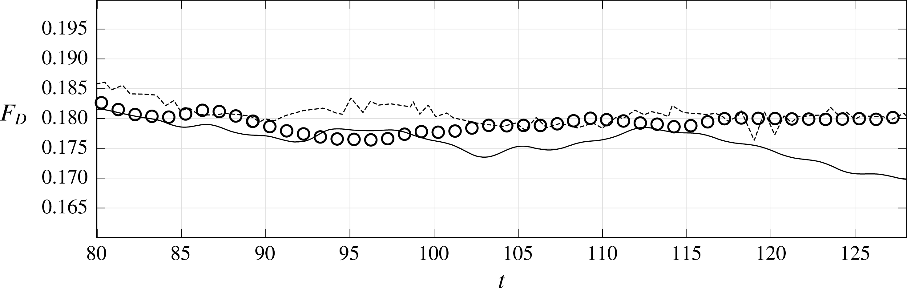
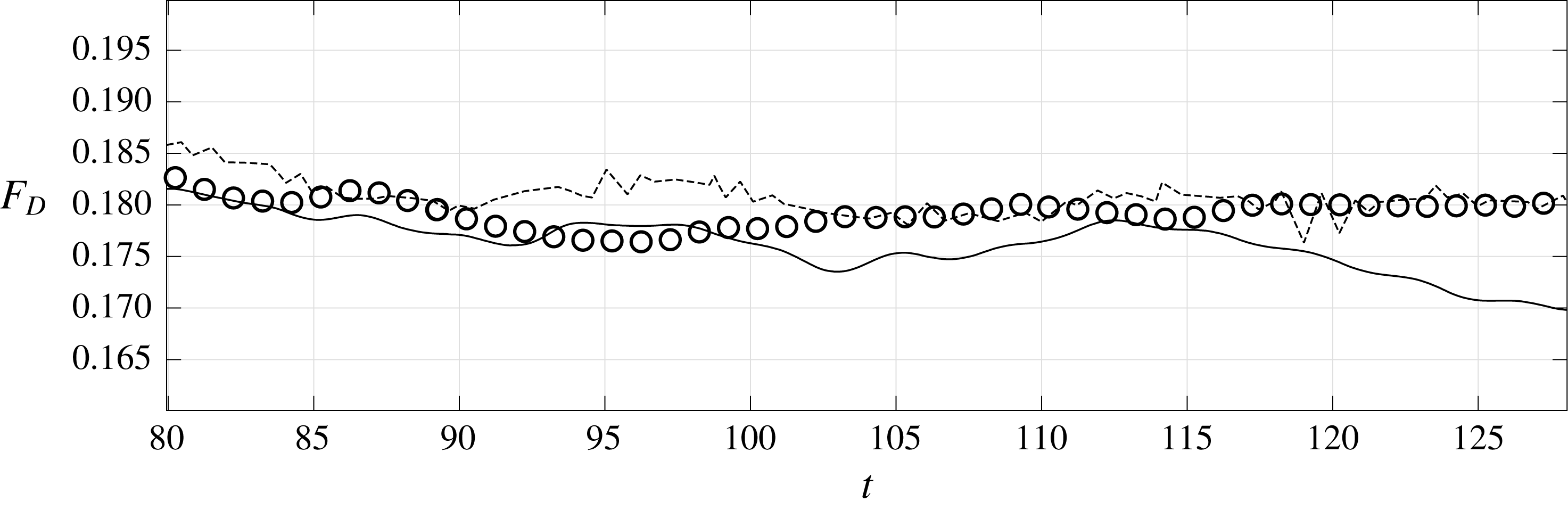
Evolution of the drag force acting on the sphere during a sample time interval, for different simulations at
 $Re^{out}=10^{3}$
. Circles: DNS around the RSP; solid line: simulation with (2.28) around the ESP; dashed line: DNS of Orr et al. (Reference Orr, Domaradzki, Spedding and Constantinescu2015) around a smooth sphere.
5.2 Turbulent regime
The condition (2.28) was developed under the assumption that the microscopic Reynolds number is not larger than
 $O(\unicode[STIX]{x1D716})$
. Many natural phenomena or engineering applications involving flows over rough surfaces take place in regimes such that
 $Re$
is larger than imposed by this theoretical restriction. To assess the limitations of the present approach, we decided to consider a case in which
 $Re^{out}$
is sufficiently large for the microscopic Reynolds number to exceed a value of order
 $\unicode[STIX]{x1D716}$
. A DNS of the flow past the RSP (still with
 $\hat{r}/R^{inn}=0.017$
,
 ${\hat{h}}/R^{inn}=\unicode[STIX]{x1D716}=0.029$
and
 $\unicode[STIX]{x1D709}=12$
) was thus set-up with
 $Re^{out}=10^{3}$
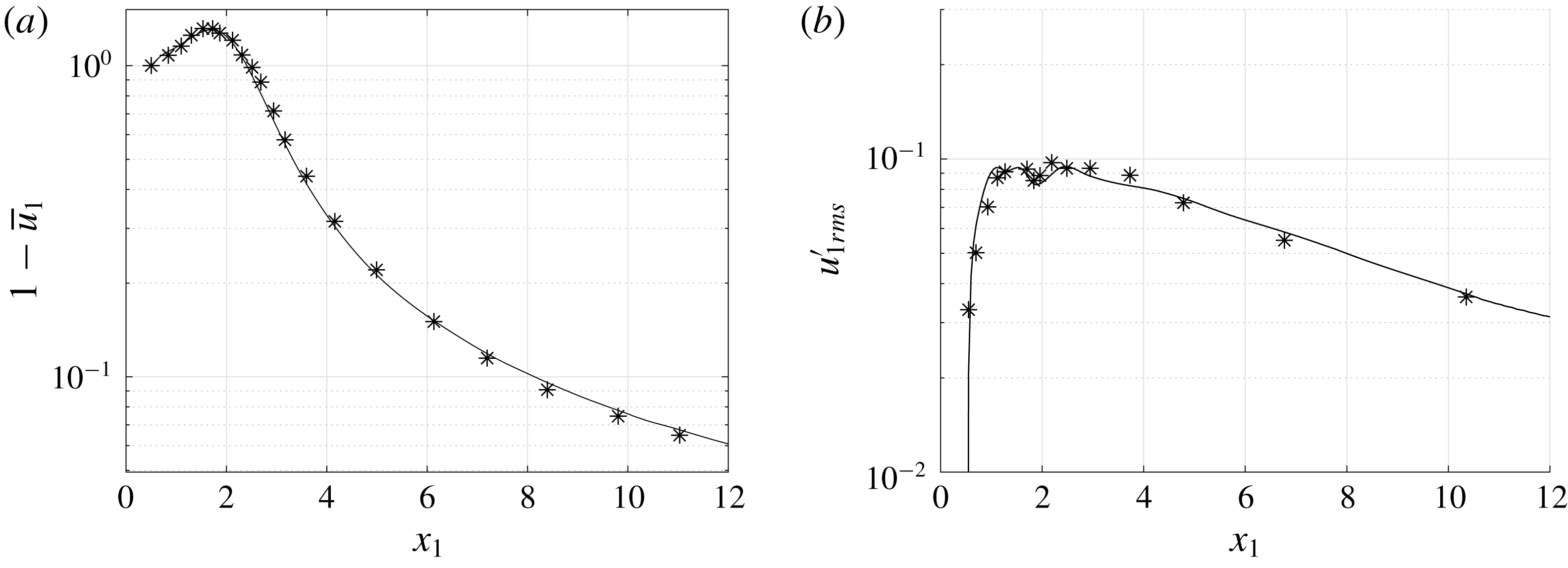
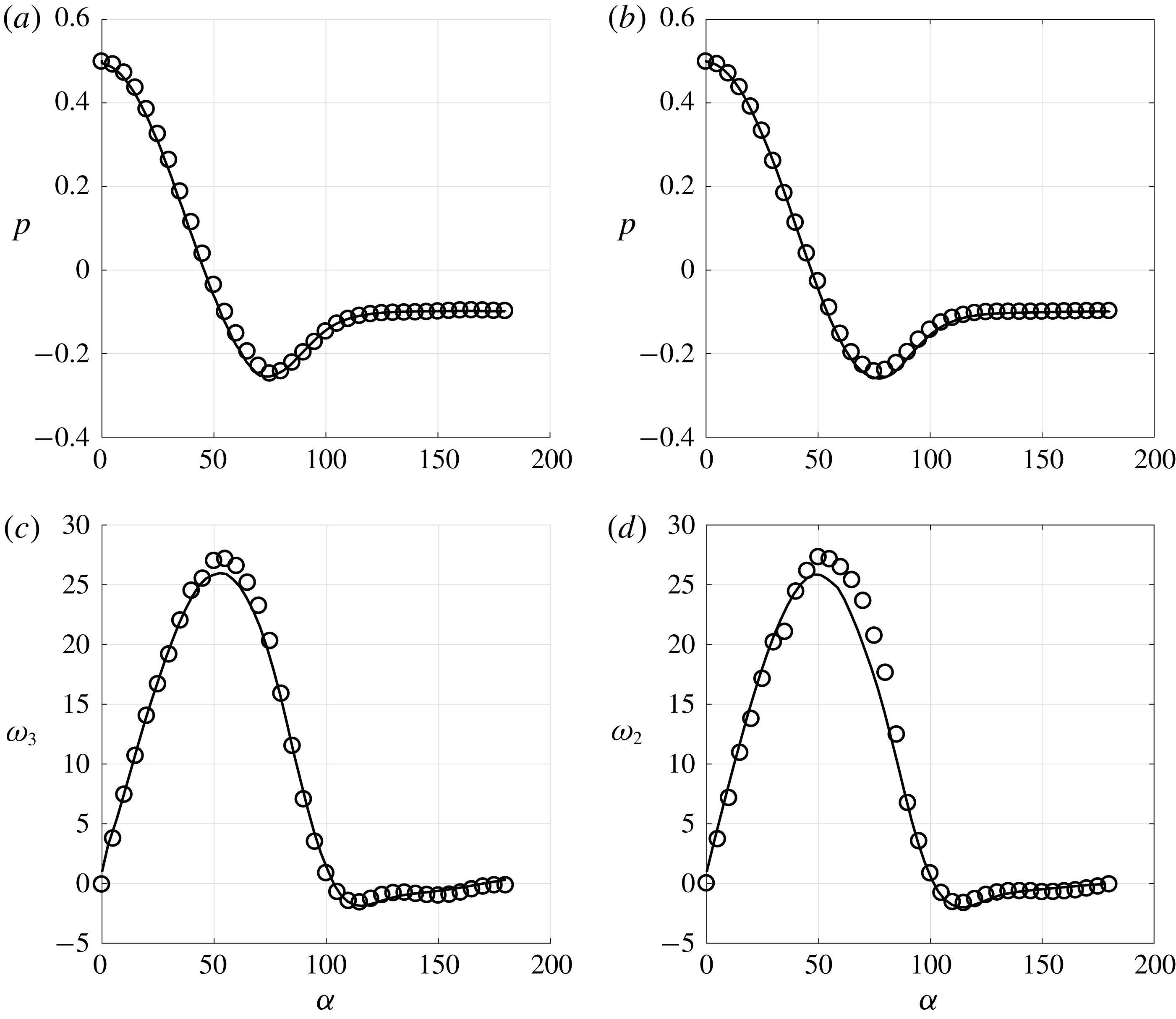
. With the chosen parameters, the flow is fully unsteady and turbulence takes place in the wake. Validations of the simulations in this regime in the case of a smooth sphere are discussed in appendix B. In particular, the longitudinal profiles of the time-averaged velocity defect and of the root-mean-square streamwise velocity fluctuation along the wake centreline are compared with the results of Orr et al. (Reference Orr, Domaradzki, Spedding and Constantinescu2015) in figure 16, revealing an excellent agreement. Figure 11 displays the evolution of the drag force acting on the RSP over a sample time interval, together with the prediction provided by the macroscopic approach based on (2.28). The evolution predicted by the DNS of Orr et al. (Reference Orr, Domaradzki, Spedding and Constantinescu2015) with a smooth sphere is also shown as a reference. The DNS and macroscopic distributions of the time-averaged surface vorticity and pressure in the cross-sectional planes aa and bb are compared in figure 12. While differences found in the pressure distributions remain small, those observed in the equatorial region on the surface vorticity are significant. Clearly (2.28) underpredicts the surface vorticity in that region, hence the viscous drag force, as was already discernible from figure 11. The poor prediction of the macroscopic approach in this case may be understood by noting that the microscale Reynolds number,
 $Re=\unicode[STIX]{x1D70C}Ul/\unicode[STIX]{x1D707}$
, characterizing the flow within each cavity embedded in the rough layer is of order one, hence much larger than
 $\unicode[STIX]{x1D716}=0.029$
. For this reason, the values of the microscopic tensor components,
 $\unicode[STIX]{x1D613}_{ijk}$
, computed on the basis of a local flow within the rough layer governed by Stokes equations, are in principle no longer valid. This limitation was already considered by Zampogna & Bottaro (Reference Zampogna and Bottaro2016) who modified the microscopic problems by incorporating Oseen’s correction to compute the permeability tensor in the case of inertia-dominated flows through rigid porous media.
Surface pressure and non-zero components of the surface vorticity within the aa (a,c) and bb (b,d) cross-sectional planes for
 $Re^{out}=10^{3}$
. Circles: DNS; solid line: macroscopic result based on (2.28).
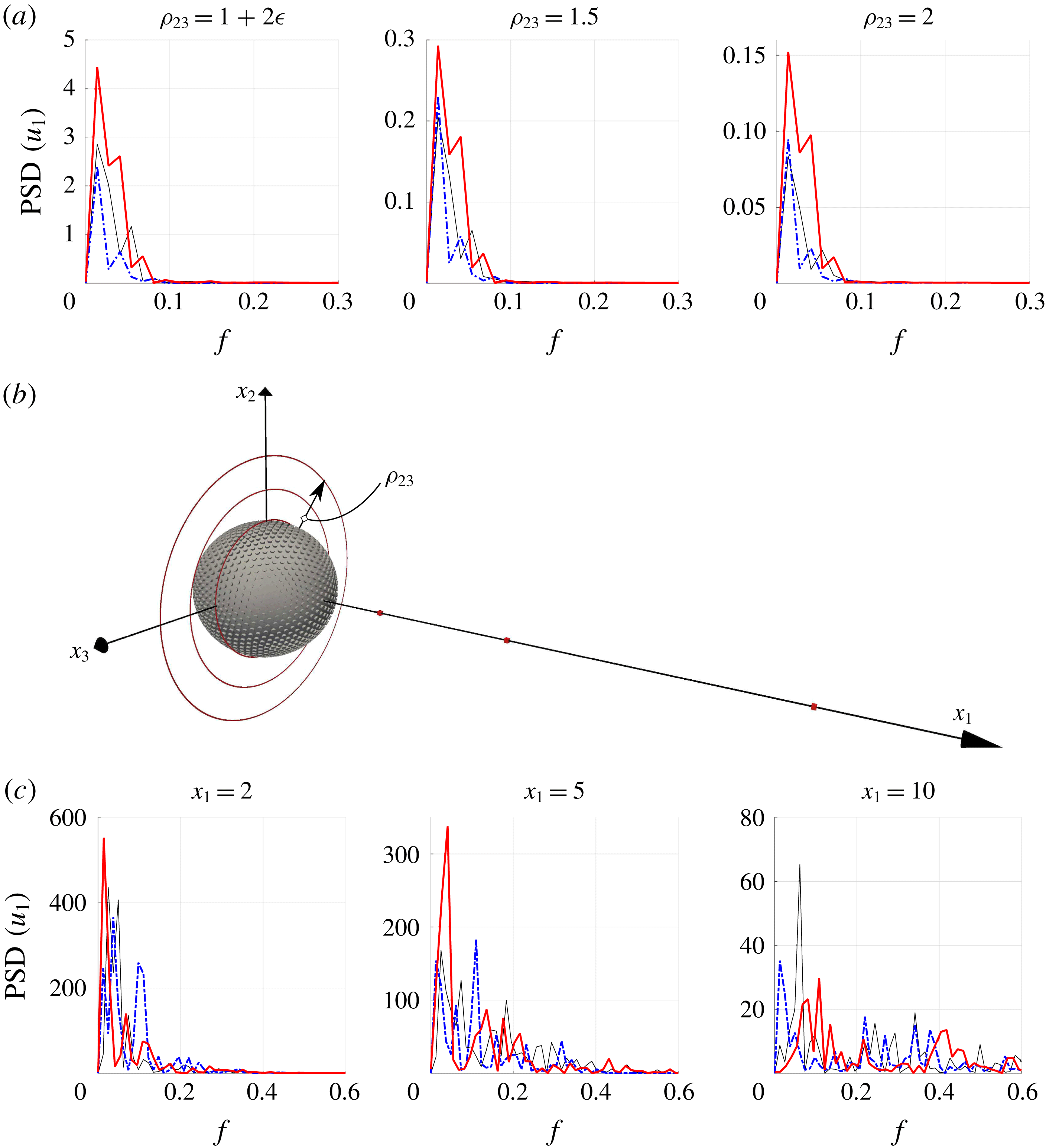
Comparison of the power spectral density (PSD) of the streamwise velocity fluctuation computed through DNS in case of a SSP (thin solid black line) or RSP (thick solid red line), and using condition (2.28) on the ESP (dash-dotted blue line). The three circles with radii
 $\unicode[STIX]{x1D70C}_{23}=(x_{2}^{2}+x_{3}^{2})^{1/2}=1+2\unicode[STIX]{x1D716}$
, 1.5 and 2 (a) and the three positions
 $x_{1}=2$
, 5 and 10 on the wake centreline at which the six spectra are evaluated (c) are indicated in red (online) in (b); frequencies are normalized with
 $U^{out}/2R$
, where
 $U^{out}$
stands for the incoming velocity.
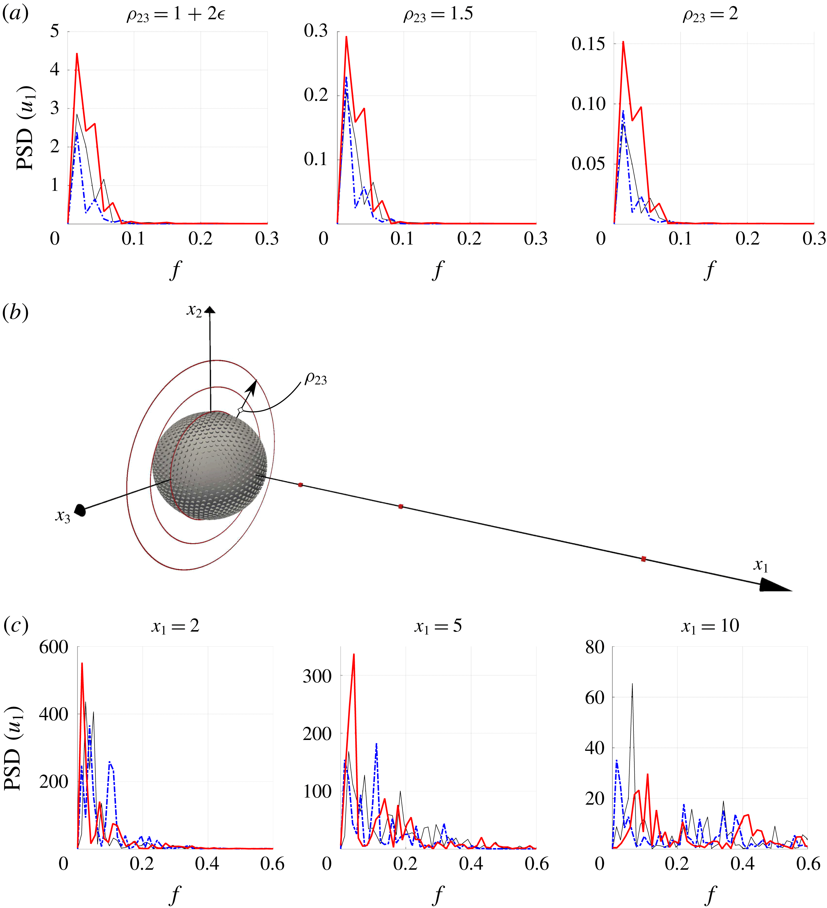
To better understand why the macroscopic model (2.28) does not faithfully predict the local characteristics of the near-surface flow in this regime, it is revealing to also examine the fluctuating field. For this purpose, we recorded the streamwise velocity,
 $u_{1}(t)$
, sampled on three circles of radii
 $\unicode[STIX]{x1D70C}_{23}=1+2\unicode[STIX]{x1D716}$
,
 $3/2$
and 2 (figure 13
a) within the equatorial plane
 $x_{1}=0$
, and on three cubic cells of volume
 $\unicode[STIX]{x1D716}^{3}$
along the wake axis, at positions
 $x_{1}=2,5$
and 10 downstream of the sphere (figure 13
c); the corresponding locations are shown in figure 13(b) (red online). To improve the statistical convergence, we averaged
 $u_{1}$
at all azimuthal positions on each circle in the equatorial plane, and at all eight vertices of each cell on the wake centreline. The streamwise velocity fluctuation,
 $u_{1}^{\prime }(t)$
, was then obtained by removing the time-average value,
 $\overline{u}_{1}$
, from
 $u_{1}(t)$
at each position. The frequency spectra of the resulting
 $u_{1}^{\prime }(t)$
signals computed at the six different locations over sampling intervals of 74 time units are displayed in figure 13. Not surprisingly, the turbulent energy is found to be a decreasing function of the distance between the sample location and the sphere, both on the equatorial plane and on the wake centreline. Moreover, it is much more intense (by more than one order of magnitude) in the wake than within the equatorial plane, i.e. within the boundary layer. For each
 $\unicode[STIX]{x1D70C}_{23}$
and simulation we can identify some dominant frequencies (Strouhal numbers) associated with energy peaks, which in the case of the flow past the SSP correspond to
 $f=0.0135$
and
 $f=0.0541$
. While the first peak is the same for the SSP and the ESP, the presence of a slip velocity on the surface of the sphere shifts the second peak backward in the latter. In the case of the flow past the RSP, three peaks are present, the dominant one corresponding to
 $f=0.0135$
, associated with a larger value of the PSD compared to those of the SSP and ESP. The energy spectrum in the wake is much richer since turbulence is developing in that region, making a clear comparison between the curves more difficult. Nevertheless it may be seen that the previously noticed mild shifting apart of blue and black curves is maintained (consider e.g. the PSD at
 $x_{1}=5$
). At
 $x_{1}=5$
, the dominant frequencies are
 $f=0.0405$
and
 $f=0.1099$
for the RSP and the ESP, respectively. In the case of the SSP, three peaks emerge at
 $f=0.0244$
,
 $f=0.0732$
and
 $f=0.1830$
. For comparison, Orr et al. (Reference Orr, Domaradzki, Spedding and Constantinescu2015) identified one dominant frequency at
 $f=0.191$
; the difference with our solution may be ascribed to the lower temporal interval sampled in this reference.
Total energy of the six PSD shown in figure 13.

More can be deduced by looking at the values of the total energy in table 4, obtained by integrating the profiles of the PSD shown in figure 13. The total energy associated with the three different boundary conditions is ordered similarly: the RSP exhibits the largest energy, followed by the SSP, then by the ESP (except at the first position,
 $x_{1}=2$
, in the wake). Compared to the reference smooth sphere, the increase of the turbulent energy found with the RSP is no surprise, since small-size protrusions are known to act as turbulence promoters. In contrast, the fact that condition (2.28) results in a decrease of the turbulent energy, even with respect to the SSP case, reveals a clear limitation of the present ‘equivalent’ boundary condition. To understand this behaviour, it must be kept in mind that if a pure shear-free condition is applied at the surface of a sphere (which in this limit is equivalent to a spherical gas bubble), no instability of the wake (hence no transition to turbulence) takes place, however large the Reynolds number might be (Magnaudet & Mougin Reference Magnaudet and Mougin2007). Increasing the slip length from zero to infinity is equivalent to gradually changing the boundary condition from no slip to shear free. If one does so while maintaining the Reynolds number fixed, the fluctuating energy is decreased until it is totally suppressed (see e.g. Legendre, Lauga & Magnaudet (Reference Legendre, Lauga and Magnaudet2009) in the case of the flow past a circular cylinder). Here, (2.28) results in a boundary condition which is intermediate between the no-slip and free-shear ones. Hence, it is no surprise that the spectra displayed in figure 13 indicate that there is less turbulence in the flow past the ESP than in those past the other two types of sphere.
The main weakness of the present theoretical model is probably that it assumes the microscopic problem to be independent of the dynamics of the external flow field. This implies in particular that the microscopic and macroscopic equations governing the equivalent boundary condition are time-independent. Obviously, this makes (2.28) unable to mimic the complex nonlinear dynamics through which wall roughnesses play an active role in the turbulence generation process. A time-dependent boundary condition in which the flow within the rough layer is coupled to the external flow field is required to lift the limitations pointed out in the above example. For this purpose, first-order inertial corrections must be taken into account in the governing equations of the microscopic problem, including the time rate-of-change term which may be large over a significant range of frequencies.
6 Concluding remarks
The main result of the present paper consists in the macroscopic boundary condition (2.28) which is applicable to general incompressible flows over microscopically rough surfaces. This condition states that the velocity components tangent to the equivalent smooth wall depend on the strain-rate tensor characterizing the outer flow at the upper limit of the rough layer. A third-order slip tensor that depends directly on the local geometry of the rough layer is associated with the strain rate of the outer flow. Within the homogenization-based framework used here, this generalized slip condition appears as the first-order correction to the usual no-slip condition. We assessed its validity via the use of DNS in a non-trivial, fully three-dimensional configuration in the presence of strong inertia effects. Macroscopic simulations based on this new boundary condition, in which the volume-averaged slip tensor is computed by solving the microscopic problem (2.21), show good agreement with the DNS results in the laminar regime. The set of equations governing this problem arise from the development of the boundary condition without further assumptions, thanks to the rational framework provided by the homogenization approach.
While the homogenization approach is most often employed to analyse problems in which time dependency and inertia are both negligible (Barenblatt, Zheltov & Kochina Reference Barenblatt, Zheltov and Kochina1960; Allaire Reference Allaire1989), it turns out to be more flexible in the present case. Indeed, the formal developments presented in § 2 and the comparisons carried out for the flow past a rough sphere in § 5.1 demonstrate that the resulting boundary condition works well, even in situations characterized by moderate-to-large Reynolds numbers. This macroscopic approach is very efficient to save computational effort and time: it greatly simplifies the building of grids aimed at computing flows involving complex surface micro-geometries, and drastically reduces the number of grid cells required to describe the flow structure close to such surfaces. To set ideas, 192 h on 500 cores at 2.8 GHz are needed to reach a converged solution of the DNS on the RSP at
 $Re^{out}=100$
, with a grid composed of
 $2.7\times 10^{7}$
elements, while the corresponding macroscopic simulation around the ESP with a comparable final resolution requires less than 4 h of computational time with a grid of less than 5 million cells. Hence, the wall approximation introduced here is particularly useful if one needs a fast feedback on global quantities such as the drag force.
However, it must be reiterated that this condition is only an
 $O(\unicode[STIX]{x1D716})$
approximation of the real microscopic behaviour. In particular, it does not allow the complex behaviour of the flow field at the microscale to be captured, as can easily be concluded by considering the fully resolved flow within the rough layer displayed in figure 9. This is also reflected in the inaccuracy with which the slip model distinguishes between pressure and viscous contributions to the force acting on the body. Two further limitations were encountered in the course of this investigation. First, the
 $O(\unicode[STIX]{x1D716})$
accuracy of the present homogenization approach does not permit to identify unambiguously the position of the equivalent surface over which (2.28) is to be applied. For instance, in the case of the flow over a sphere considered in § 5.1, the tests carried out with the two limit values of the equivalent radius,
 $R^{inn}$
and
 $R^{out}$
, yielded similar results. This indicates that seeking the exact position of the equivalent smooth surface within the interval
 $[R^{inn},R^{out}]$
is irrelevant at this level of approximation. A higher-order theory is required if a higher accuracy is needed. A second limitation is the following: since the equivalent boundary condition was developed under the assumption
 $Re\lesssim O(\unicode[STIX]{x1D716})$
, it was no surprise to observe that the accuracy of the predictions decreases severely as larger outer Reynolds numbers are considered. We have found that the equivalent boundary condition is still able to capture correctly the overall behaviour of the outer flow, but significantly underestimates the surface vorticity (hence the shear stress) near the sphere’s equator, resulting in an underestimate of the overall drag force. Moreover, the analysis of the turbulent fluctuations carried out in § 5.2 revealed that, instead of predicting an increase of the turbulence level in the case of the RSP, the first-order macroscopic approach predicts that the fluctuating energy is less than in the reference SSP case. Clearly, inertia effects cannot be ignored any longer in the calculation of the microscopic tensors in this regime. An inertial coupling with the dynamic properties of the external macroscopic flow must be included in the microscopic problems, in order for the modified slip condition to mimic properly the role of the rough layer as turbulence promoter.
With the roughness distribution and the flow regimes considered here, only small variations of the global forces acting on a rough spherical particle were noticed, compared to a smooth sphere of the same size. Nonetheless, the boundary condition (2.28) provides a powerful and versatile tool to modify – at least as a first approximation – the shape and distribution of the protrusions, for example to optimize the forces acting on a given rough body. More complex and realistic surfaces in which the assumption of periodicity at the microscopic level is relaxed may be considered in the future by extending the derivation of the slip tensor in the framework of stochastic homogenization theory (Cottereau Reference Cottereau2012; Bella et al. Reference Bella, Ferhman, Fischer and Otto2016). Another possibility to be explored is that of a modification of the microscopic behaviour of the rough boundary through the introduction of a local hydrophobic treatment capable of trapping air nanobubbles within the cavities of the rough wall.
Acknowledgements
The authors thank the anonymous referees for their many valuable suggestions, and the IDEX Foundation of the University of Toulouse for the financial support granted to the last author under the project ‘Attractivity Chairs’. This work was granted access to the HPC resources of the CALMIP supercomputing centre under the allocation 2017-P17021.
Appendix A. Extension of the boundary condition to generic surfaces
Equation (2.28) is a general relation without any limitation on the geometry of the surface to which it is applied. However, the computed slip tensors considered in § 2 referred only to planar surfaces, since we assumed the tangential and normal-to-the-surface directions
 $(\boldsymbol{t}_{1},\boldsymbol{t}_{2},\boldsymbol{n})$
vectors to be constant and identical to the Cartesian unit vectors
 $(\boldsymbol{e}_{1},\boldsymbol{e}_{2},\boldsymbol{e}_{3})$
. For a non-planar surface
 $\mathbb{E}\mathbb{S}$
, equation (2.21) may still be used provided that (i)
 $\mathbb{S}$
is covered by a periodic lattice, and (ii) the separation of scales is sufficiently large for the curvature of the surface at the microscopic level to be negligible. Thanks to (i),
 ${\mathcal{L}}_{ijk}$
is constant if expressed in terms of the local frame built on the tangent and normal unit vectors
 $(\boldsymbol{t}_{1},\boldsymbol{t}_{2},\boldsymbol{n})$
, but this is no longer the case if the coordinate system is changed to an arbitrary one. Thanks to (ii), the problem (2.21) yields
 $$\begin{eqnarray}\boldsymbol{{\mathcal{L}}}={\mathcal{L}}_{113}\boldsymbol{t}_{1}\wedge \boldsymbol{t}_{1}\wedge \boldsymbol{n}+{\mathcal{L}}_{223}\boldsymbol{t}_{2}\wedge \boldsymbol{t}_{2}\wedge \boldsymbol{n},\end{eqnarray}$$
where
 $\wedge$
denotes the tensor product (
 $\boldsymbol{a}\wedge \boldsymbol{b}:=a_{i}b_{j}$
). To express
 ${\mathcal{L}}_{ijk}$
in Cartesian coordinates, as in (2.28), we need to define the mapping
 $$\begin{eqnarray}\unicode[STIX]{x1D6EF}:\mathbb{R}^{3}\rightarrow \mathbb{S}\quad \text{such that }(\boldsymbol{e}_{1},\boldsymbol{e}_{2},\boldsymbol{e}_{3})\rightarrow (\boldsymbol{t}_{1},\boldsymbol{t}_{2},\boldsymbol{n}).\end{eqnarray}$$
Applying
 $\unicode[STIX]{x1D6EF}$
to (A 1), we find the Cartesian expression of the tensor components. In particular, by virtue of the definition of the
 $\wedge$
product, the symmetry properties remain unaltered. In the present case, these symmetries imply
 $$\begin{eqnarray}{\mathcal{L}}_{ijk}={\mathcal{L}}_{jik}={\mathcal{L}}_{ikj}.\end{eqnarray}$$
In § 4 we used (2.28) to impose a non-zero slip over a sphere. In this case, the mapping
 $\unicode[STIX]{x1D6EF}$
is defined as
 $$\begin{eqnarray}\displaystyle & \displaystyle \boldsymbol{t}_{1}(\boldsymbol{e}_{1},\boldsymbol{e}_{2},\boldsymbol{e}_{3})=-\text{sin}\unicode[STIX]{x1D703}\,\boldsymbol{e}_{1}+\cos \unicode[STIX]{x1D703}\,\boldsymbol{e}_{2}, & \displaystyle\end{eqnarray}$$
 $$\begin{eqnarray}\displaystyle & \displaystyle \boldsymbol{t}_{2}(\boldsymbol{e}_{1},\boldsymbol{e}_{2},\boldsymbol{e}_{3})=\cos \unicode[STIX]{x1D703}\cos \unicode[STIX]{x1D719}\boldsymbol{e}_{1}+\sin \unicode[STIX]{x1D703}\cos \unicode[STIX]{x1D719}\boldsymbol{e}_{2}-\sin \unicode[STIX]{x1D719}\boldsymbol{e}_{3}, & \displaystyle\end{eqnarray}$$
 $$\begin{eqnarray}\displaystyle & \displaystyle \boldsymbol{n}(\boldsymbol{e}_{1},\boldsymbol{e}_{2},\boldsymbol{e}_{3})=\cos \unicode[STIX]{x1D703}\sin \unicode[STIX]{x1D719}\boldsymbol{e}_{1}+\sin \unicode[STIX]{x1D703}\sin \unicode[STIX]{x1D719}\boldsymbol{e}_{2}+\cos \unicode[STIX]{x1D719}\boldsymbol{e}_{3}, & \displaystyle\end{eqnarray}$$
where the angles
 $\unicode[STIX]{x1D703}$
and
 $\unicode[STIX]{x1D719}$
identify the local position on the sphere surface. In Cartesian coordinates:
 $\unicode[STIX]{x1D703}=\text{tan}^{-1}(x_{2}/x_{1})$
for
 $x_{1}\geqslant 0$
,
 $\unicode[STIX]{x1D703}=\unicode[STIX]{x03C0}+\tan ^{-1}(x_{2}/x_{1})$
for
 $x_{1}<0$
and
 $\unicode[STIX]{x1D719}=\cos ^{-1}(x_{3}/R)$
. Substituting (A 4)–(A 6) in (A 1), we obtain
 $\boldsymbol{{\mathcal{L}}}$
for a spherical surface.
In § 2, we noticed that the wall-normal velocity is zero in (2.27) if the no-slip condition applies. This behaviour is valid also after a change of coordinates. This is easily verified by noting that
 $\boldsymbol{t}_{1}\boldsymbol{\cdot }\boldsymbol{n}=\boldsymbol{t}_{2}\boldsymbol{\cdot }\boldsymbol{n}=0$
and, consequently,
 $$\begin{eqnarray}\boldsymbol{n}\boldsymbol{\cdot }\boldsymbol{t}_{1}\wedge \boldsymbol{t}_{1}\wedge \boldsymbol{n}=\boldsymbol{n}\boldsymbol{\cdot }\boldsymbol{t}_{2}\wedge \boldsymbol{t}_{2}\wedge \boldsymbol{n}=0.\end{eqnarray}$$
Projecting (2.28) along
 $\boldsymbol{n}$
and using (A 7), the normal velocity component is then seen to vanish.
Appendix B. Technical aspects of the computations
The numerical solutions discussed in this paper were obtained using the finite volume open source software OpenFOAM (http://www.openfoam.org). In this appendix we summarize the issues related to the numerical solution of the microscopic and macroscopic problems.
B.1 Implementation of the condition (2.28)
To compute the flow past the ESP, the boundary condition (2.28) was transformed into a non-homogeneous Neumann condition by implementing it in the explicit iterative form
 $$\begin{eqnarray}\frac{\unicode[STIX]{x2202}u_{i}^{(m)}}{\unicode[STIX]{x2202}x_{j}}n_{j}=\frac{\unicode[STIX]{x2202}u_{i}^{(m-1)}}{\unicode[STIX]{x2202}x_{j}}n_{j}-u_{i}^{(m-1)}+\unicode[STIX]{x1D716}{\mathcal{L}}_{ilk}\left.\left(\frac{\unicode[STIX]{x2202}u_{l}^{(m-1)}}{\unicode[STIX]{x2202}x_{k}}+\frac{\unicode[STIX]{x2202}u_{k}^{(m-1)}}{\unicode[STIX]{x2202}x_{l}}\right)\right|_{\mathbb{ES}},\end{eqnarray}$$
where
 $m$
denotes the temporal index and
 $n_{j}$
is the outer unit normal to the
 $\mathbb{E}\mathbb{S}$
surface.
B.2 Convergence of the microscopic results
The spatial convergence of the steady solution of problem (2.21) was checked. Figure 14 displays three different spatial discretizations of the microscopic cell for the case
 $r=0.5751$
and
 $h=1$
. The grids were built with the routine snappyHexMesh, using
 $n=25$
, 50 and 100 cells per unit length, respectively. The values of
 ${\mathcal{L}}_{113}$
reported in table 5 are computed with a cell such that
 $l_{3}=2\sqrt{3}$
and indicate convergence for
 $n=50$
.
Cut of the microscopic elementary cell at
 $x_{3}=0.5$
. The three different grids used to test the spatial convergence are displayed. They involve 25, 50 and 100 cells per unit length, respectively.
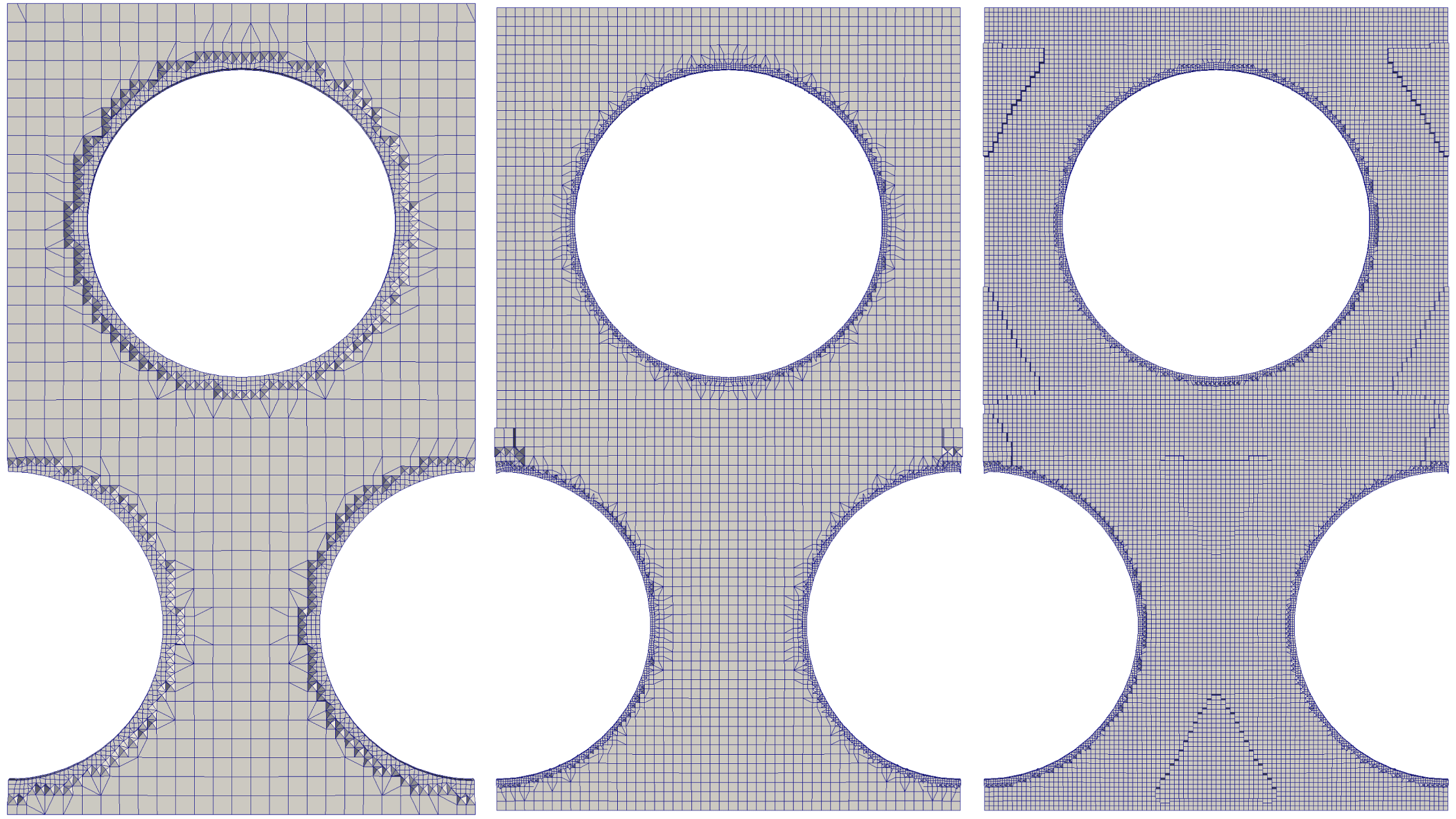
Drag force on a SSP in the case of the small (S) and large (B) computational domains (
 $Re^{out}=100$
). The numbers on the horizontal axis refer to different grid resolutions: from
 $1.8\times 10^{4}$
cells (S1) to
 $6.2\times 10^{6}$
cells (S4 and B4).
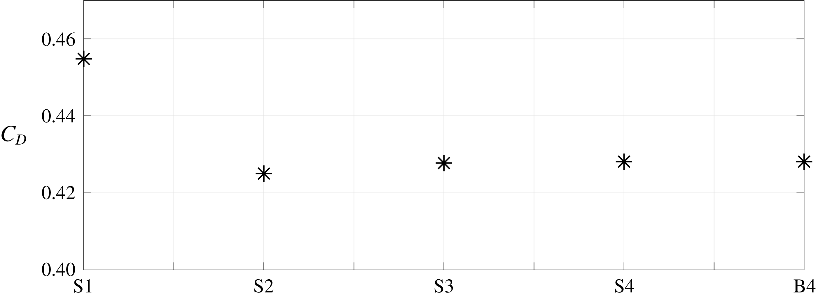
Spatial convergence of
 ${\mathcal{L}}_{113}$
with respect to the grids shown in figure 14 and
 $l_{3}=2\sqrt{3}$
. The number
 $n$
denotes the number of cells per unit length.

B.3 Validation of the macroscopic configuration and convergence of the results
To validate the solver used to compute the flow past both the RSP and ESP, we considered the flow past a SSP, with a no-slip condition at its surface and
 $Re^{out}=100$
. Figure 15 shows the total drag force (
 $F_{D}$
) acting on a SSP with unit radius, when the resolution and the size of the computational domain are varied. The configurations denoted with ‘S’ refer to a small domain with size
 $100\times 40\times 40$
, while ‘B’ stands for a bigger domain with size
 $200\times 80\times 80$
. The numbers refer to different grid resolutions. After having confirmed grid convergence for the S configuration, we checked the influence of the domain size by switching to the B configuration. As can be inferred from figure 15, the S3 configuration already estimates well the drag force acting on the SSP. Computing flow statistics in the turbulent flow past a SSP at
 $Re^{out}=1000$
required a large sampling time. More precisely, the statistics were carried out using a time window of 74 units with 100 samples per unit. Figure 16 shows the longitudinal profiles along the wake centreline of two quantities of primary interest to assess the quality of the computation, namely the mean velocity defect and the root-mean-square value of the streamwise velocity fluctuation. Both profiles are found to agree well with the results of Orr et al. (Reference Orr, Domaradzki, Spedding and Constantinescu2015) up to
 $x_{1}\gtrsim 10$
.
Statistical properties of the turbulent flow in the wake past a SSP at
 $Re^{out}=1000$
. Longitudinal profiles of (a) the mean velocity defect,
 $1-\overline{u}_{1}$
(the incoming velocity is set to unity), and (b) the root-mean-square value of the streamwise velocity fluctuation,
 $u_{1}^{\prime }$
. The solid line corresponds to the DNS results of Orr et al. (Reference Orr, Domaradzki, Spedding and Constantinescu2015).
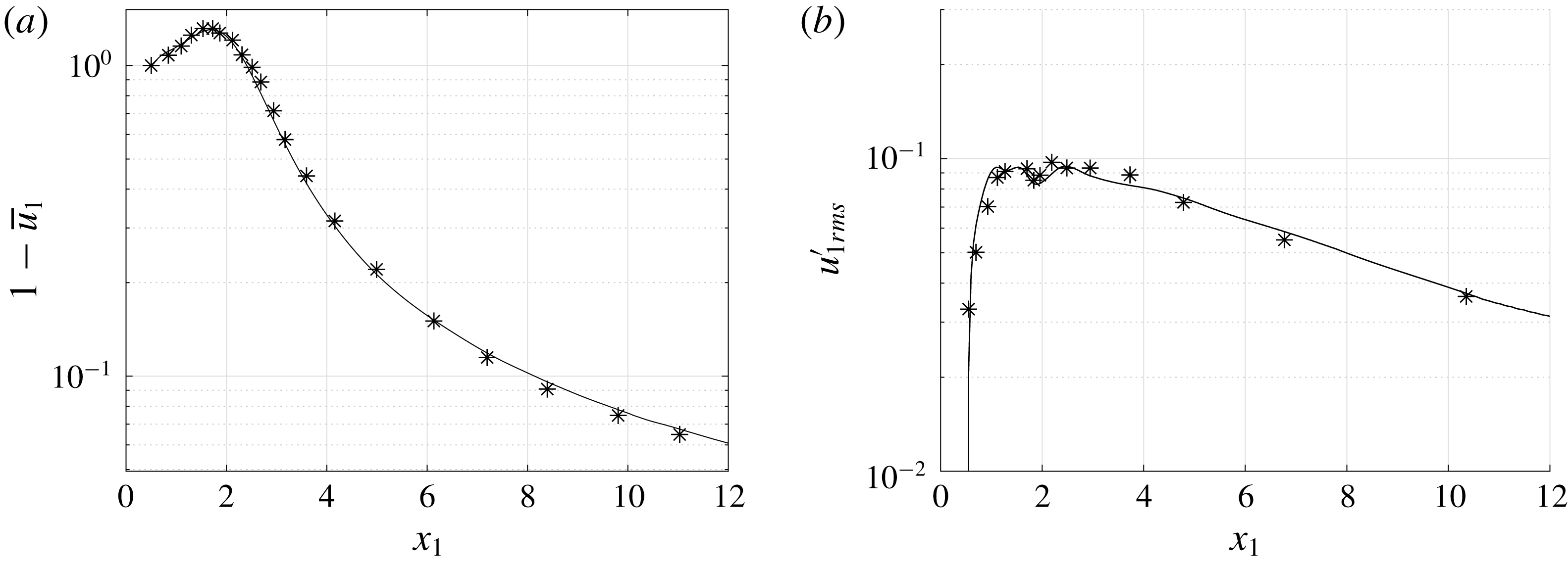
Zoom of the computational grid around a RSP, composed of
 $2.7\times 10^{7}$
cells.
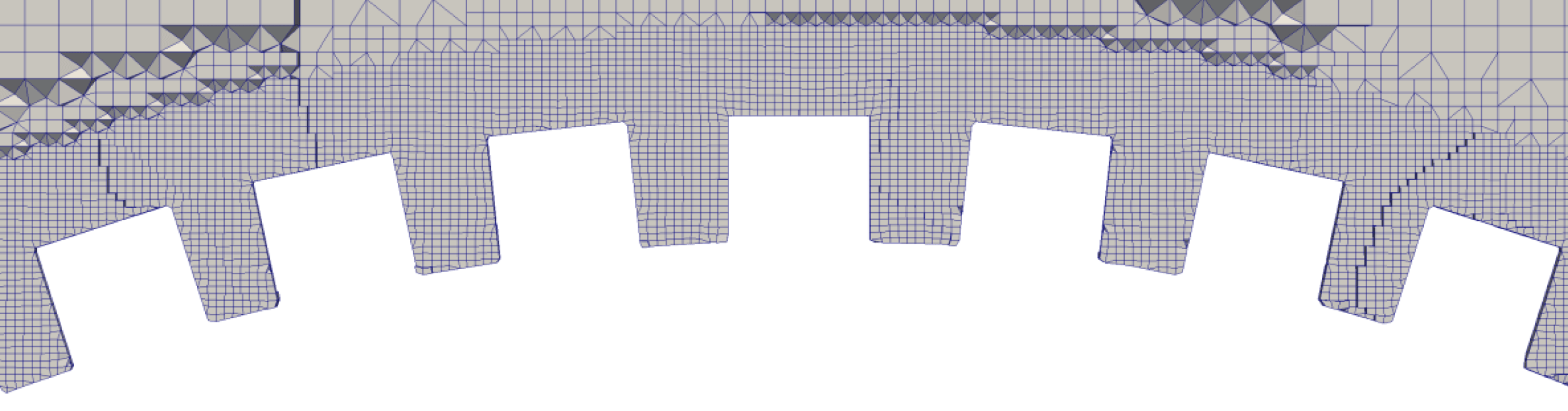
B.4 Evaluation of the forces on the RSP
To compute the flow past a RSP, two domains were employed, made of approximately
 $1.5\times 10^{7}$
and
 $2.7\times 10^{7}$
cells, respectively. No significant change in the local and global forces acting on the sphere was noticed. A large number of computational cells is required to properly solve the fluid flow at the scale of the protrusions. A zoom of the grid close to the sphere surface is provided in figure 17. In this case, the grid is made of
 $2.7\times 10^{7}$
cells and the code is run using 500 cores in parallel.
To determine the forces at the particle surface, two methods were used. The first of them is characteristic of a pointwise approach, with pressure and viscous forces evaluated over each cell of the computational grid used to discretize the surface, then integrated over the whole RSP. The corresponding values (shown in table 2) are meaningful in a pointwise sense, aside from the value of
 $\unicode[STIX]{x1D6FC}_{S}$
for the RSP which is an average value because of the lack of rotational symmetry of the rough layer with respect to the
 $x_{1}$
-axis.
The second method is the macroscopic counterpart of the above approach. It consists of the following steps:
(i) The rough layer is divided into elementary microscopic cells.
(ii) Pressure and viscous stresses are integrated over each cell, providing locally averaged forces.
(iii) Since the ensemble of the microscopic cells covers the whole surface of the spherical particle, each cell is univocally identified with a portion of the smooth sphere underlying the rough layer (which ideally corresponds to a macroscopic point). This allows an accurate mapping between the RSP and the ESP to be established.
(iv) The locally averaged forces are projected onto the portions of the ESP identified at the previous step.
(v) The values obtained through this projection are integrated over the ESP surface.
This procedure, the results of which are shown in table 3, makes it possible to compute ‘macroscopic’ forces acting on a RSP comparable with those obtained by imposing (2.28) on the surface of the ESP.