2.1 Base-flow Rankine–Hugoniot equations

Consider a planar detonation front whose relative speed with respect to the upstream flow is $u_{o}^{\prime }>a_{o}^{\prime }$ , where the speed of sound $a_{o}^{\prime }$ is modelled with the perfect-gas assumption $a_{o}^{\prime 2}=\unicode[STIX]{x1D6FE}p_{o}^{\prime }/\unicode[STIX]{x1D70C}_{o}^{\prime }$ . The changes in the flow variables across the front are obtained by integrating the conservation equations in the streamwise direction, yielding

(2.1a ) $$\begin{eqnarray}\displaystyle & \displaystyle \unicode[STIX]{x1D70C}_{o}^{\prime }u_{o}^{\prime }=\unicode[STIX]{x1D70C}_{d}^{\prime }u_{d}^{\prime }, & \displaystyle\end{eqnarray}$$

(2.1b ) $$\begin{eqnarray}\displaystyle & \displaystyle p_{o}^{\prime }+\unicode[STIX]{x1D70C}_{o}^{\prime }u_{o}^{\prime 2}=p_{d}^{\prime }+\unicode[STIX]{x1D70C}_{d}^{\prime }u_{d}^{\prime 2}, & \displaystyle\end{eqnarray}$$

(2.1c ) $$\begin{eqnarray}\displaystyle & \displaystyle h_{o}^{\prime }+{\textstyle \frac{1}{2}}u_{o}^{\prime 2}=h_{d}^{\prime }+{\textstyle \frac{1}{2}}u_{d}^{\prime 2}, & \displaystyle\end{eqnarray}$$

$o$

$d$

$u^{\prime }$

$\unicode[STIX]{x1D70C}^{\prime }$

$p^{\prime }$

$h^{\prime }$

$\unicode[STIX]{x1D6FE}$

(2.2) $$\begin{eqnarray}h_{d}^{\prime }-h_{o}^{\prime }=\frac{\unicode[STIX]{x1D6FE}}{\unicode[STIX]{x1D6FE}-1}\frac{p_{d}^{\prime }}{\unicode[STIX]{x1D70C}_{d}^{\prime }}-\frac{\unicode[STIX]{x1D6FE}}{\unicode[STIX]{x1D6FE}-1}\frac{p_{o}^{\prime }}{\unicode[STIX]{x1D70C}_{o}^{\prime }}+\unicode[STIX]{x0394}h_{f}^{o},\end{eqnarray}$$

provided that exothermic effects occur within a thin layer right behind the shock wave. Ideally, the total energy per unit mass delivered to the fluid particles is given by the difference between the formation enthalpies of the products and reactants $\unicode[STIX]{x0394}h_{f}^{o}$ .

Although the heat release rate is strongly affected by local properties behind the precursor shock wave, mainly the temperature, the overall heat released is slightly affected by the thermodynamic conditions in the reaction layer. Nonetheless, sufficiently strong changes in pressure or temperature could promote the formation of different radicals, in which case the global thermodynamic equilibrium involving a combination of different species could affect the overall amount of heat released. One example is nitrogen in air, which cannot be considered inert when the temperature is sufficiently high. Direct computations of one-dimensional detonations for stoichiometric methane–air mixtures, performed independently with models (McBride, Zehe & Gordon Reference McBride, Zehe and Gordon2002; Browne, Ziegler & Shepherd Reference Browne, Ziegler and Shepherd2008), show that temperature tends to reduce global heat release while pressure contributes with an opposite effect. Other phenomena beyond chemical reactions may affect the overall heat released, such as the final state (liquid or gas) of the H $_{2}$ O, or radiation losses that depend on the temperature. In particular, phase changes can affect the heat released when the fuel is a diluted spray (Williams Reference Williams1961, Reference Williams1985; Smolders & van Dongen Reference Smolders and van Dongen1992; Guha Reference Guha1994; Martínez-Ruiz et al. Reference Martínez-Ruiz, Urzay, Sánchez, Liñan and Williams2013; Smirnov et al. Reference Smirnov, Betelin, Kushnirenko, Nikitin, Dushin and Nerchenko2013; Vimercati, Gori & Guardone Reference Vimercati, Gori and Guardone2018). Along with these applications, the astrophysical context opens a wide range of possibilities for non-adiabatic waveforms, such as the thermonuclear detonations formed in Type Ia supernovae whose potential nuclear fuel depends on the density, which peaks just behind the precursor shock (Khokhlov Reference Khokhlov1989; Khokhlov, Oran & Wheeler Reference Khokhlov, Oran and Wheeler1997; Gamezo et al. Reference Gamezo, Khokhlov and Oran2004; Wright et al. Reference Wright, Nagaraj, Kneller, Scholberg and Seitenzahl2016; Ami Glasner et al. Reference Ami Glasner, Livne, Steinberg, Yalinewich and Truran2018; Röpke & Sim Reference Röpke and Sim2018).

When the detonation is driven by reactions that depend on local thermodynamic functions, the heat released depends on the shock strength. Certainly, any particular case would call for a specific model to compute the variations in the global heat released with the shock intensity. Because this dependence is presumably small, a linear perturbation analysis could be employed to write

(2.3) $$\begin{eqnarray}\unicode[STIX]{x0394}h_{f}^{o}=\unicode[STIX]{x0394}h_{f}^{o}|_{o}+\left.{\displaystyle \frac{\unicode[STIX]{x2202}\unicode[STIX]{x0394}h_{f}^{o}}{\unicode[STIX]{x2202}T}}\right|_{o}\unicode[STIX]{x1D6FF}T+\left.{\displaystyle \frac{\unicode[STIX]{x2202}\unicode[STIX]{x0394}h_{f}^{o}}{\unicode[STIX]{x2202}p}}\right|_{o}\unicode[STIX]{x1D6FF}p,\end{eqnarray}$$

as the variable heat of reaction delivered to the fluid particles. Reactions that can depend on the bulk density, such as those involved in thermonuclear detonations, can be easily incorporated into (2.3) with the corresponding equation of state.

The heat released is conveniently scaled with the fresh-gas properties. Therefore, ${\mathcal{H}}_{0}=(\unicode[STIX]{x1D6FE}^{2}-1)\unicode[STIX]{x0394}h_{f}^{o}/(2a_{o}^{\prime 2})$ defines the dimensionless order-of-unity heat released. Because the pressure and temperature scale with the shock strength squared for sufficiently strong shocks, such as those expected in detonations, variations of the global heat released with the thermodynamic variables can be collected in the small term $\unicode[STIX]{x1D716}$ , where

(2.4) $$\begin{eqnarray}{\mathcal{H}}_{0}=q(1+\unicode[STIX]{x1D716}{\mathcal{M}}_{o}^{2})\end{eqnarray}$$

defines the shock-dependent dimensionless heat released. The ratio ${\mathcal{M}}_{o}=u_{o}^{\prime }/a_{o}^{\prime }$ defines the Mach number of the detonation wave, and $q$ is the constant heat released contribution, i.e. when it does not depend on the shock strength. Note that the factor $\unicode[STIX]{x1D716}\ll 1$ can be either positive, when the heat released is positively correlated with the shock strength, or negative, when it is negatively correlated.

Simple manipulation of (2.1a )–(2.1c ) provides the jump equations across the reaction front, namely,

(2.5) $$\begin{eqnarray}\displaystyle & \displaystyle {\mathcal{R}}_{d}=\frac{\unicode[STIX]{x1D70C}_{d}^{\prime }}{\unicode[STIX]{x1D70C}_{o}^{\prime }}=\frac{u_{o}^{\prime }}{u_{d}^{\prime }}=\frac{(\unicode[STIX]{x1D6FE}+1){\mathcal{M}}_{o}^{2}}{(\unicode[STIX]{x1D6FE}-\unicode[STIX]{x1D705}){\mathcal{M}}_{o}^{2}+1}, & \displaystyle\end{eqnarray}$$

(2.6) $$\begin{eqnarray}\displaystyle & \displaystyle {\mathcal{P}}_{d}=\frac{p_{d}^{\prime }}{p_{o}^{\prime }}=1-\unicode[STIX]{x1D6FE}{\mathcal{M}}_{o}^{2}{\displaystyle \frac{{\mathcal{R}}_{d}-1}{{\mathcal{R}}_{d}}}=\frac{\unicode[STIX]{x1D6FE}{\mathcal{M}}_{o}^{2}(1+\unicode[STIX]{x1D705})+1}{\unicode[STIX]{x1D6FE}+1}, & \displaystyle\end{eqnarray}$$

for density and pressure, respectively. The Mach number of the burnt-gas flow is

(2.7) $$\begin{eqnarray}{\mathcal{M}}_{d}=\frac{u_{d}^{\prime }}{a_{d}^{\prime }}={\displaystyle \frac{1}{\sqrt{\unicode[STIX]{x1D6FE}{\mathcal{R}}_{d}{\mathcal{P}}_{d}}}}=\left[\frac{(\unicode[STIX]{x1D6FE}-\unicode[STIX]{x1D705}){\mathcal{M}}_{o}^{2}+1}{\unicode[STIX]{x1D6FE}{\mathcal{M}}_{o}^{2}(1+\unicode[STIX]{x1D705})+1}\right]^{1/2},\end{eqnarray}$$

with the function

(2.8) $$\begin{eqnarray}\unicode[STIX]{x1D705}=[(1-{\mathcal{M}}_{o}^{-2})^{2}-4{\mathcal{H}}_{0}{\mathcal{M}}_{o}^{-2}]^{1/2},\end{eqnarray}$$

accounting for the dimensionless non-adiabatic parameter ${\mathcal{H}}_{0}$ . For non-reacting shock waves, $\unicode[STIX]{x1D705}=1-{\mathcal{M}}_{o}^{-2}$ , which simplifies (2.5)–(2.7) to the well-known adiabatic RH relationships. Note that the form of (2.5)–(2.8) is similar to those found in any classical reference on combustion (see Williams Reference Williams1985; Clavin & Searby Reference Clavin and Searby2016); the only difference here is the way the function ${\mathcal{H}}_{0}$ is modelled in (2.4).

The so-called Chapman–Jouguet (CJ) regime defines the minimum detonation strength associated with a given energy release, namely,

(2.9) $$\begin{eqnarray}{\mathcal{M}}_{cj}=\sqrt{{\displaystyle \frac{1}{1+2q-2\sqrt{q(1+q+\unicode[STIX]{x1D716})}}}}\sim {\mathcal{M}}_{cj}^{\unicode[STIX]{x1D716}=0}\left[1+\unicode[STIX]{x1D716}{\displaystyle \frac{(\sqrt{1+q}+\sqrt{q})^{2}}{2\sqrt{q+1}}}\right],\end{eqnarray}$$

where ${\mathcal{M}}_{cj}^{\unicode[STIX]{x1D716}=0}=\sqrt{1+q}+\sqrt{q}$ is the CJ propagation Mach number when the heat released does not depend on the shock intensity, $\unicode[STIX]{x1D716}=0$ . In this regime, the flow behind the reacting shock is sonic, ${\mathcal{M}}_{d}=1$ , and the detonation front decouples from the downstream condition; thereby, its motion is self-sustained by the expansion of the products resulting from the exothermic transformation. As expected, a positive correlation of the heat release with the shock intensity increases the self-propagating velocity ${\mathcal{M}}_{cj}$ , while the contrary occurs for $\unicode[STIX]{x1D716}<0$ .

The RH curve relates the pressure jump to the mass compression ratio (or specific volume) across the detonation wave. This function,

(2.10) $$\begin{eqnarray}{\mathcal{P}}_{d}={\displaystyle \frac{(\unicode[STIX]{x1D6FE}-1)({\mathcal{R}}_{d}-1)[\unicode[STIX]{x1D6FE}+1-(\unicode[STIX]{x1D6FE}-1){\mathcal{R}}_{d}]+4{\mathcal{R}}_{d}q[\unicode[STIX]{x1D6FE}({\mathcal{R}}_{d}-1)-{\mathcal{R}}_{d}\unicode[STIX]{x1D716}]}{(\unicode[STIX]{x1D6FE}-1)({\mathcal{R}}_{d}-1)[(\unicode[STIX]{x1D6FE}+1){\mathcal{R}}_{d}-\unicode[STIX]{x1D6FE}+1]-4{\mathcal{R}}_{d}^{2}q\unicode[STIX]{x1D716}}},\end{eqnarray}$$

is explicitly written for convenience in defining the auxiliary function (1.2) when it is written in terms of dimensionless variables; see (2.16).

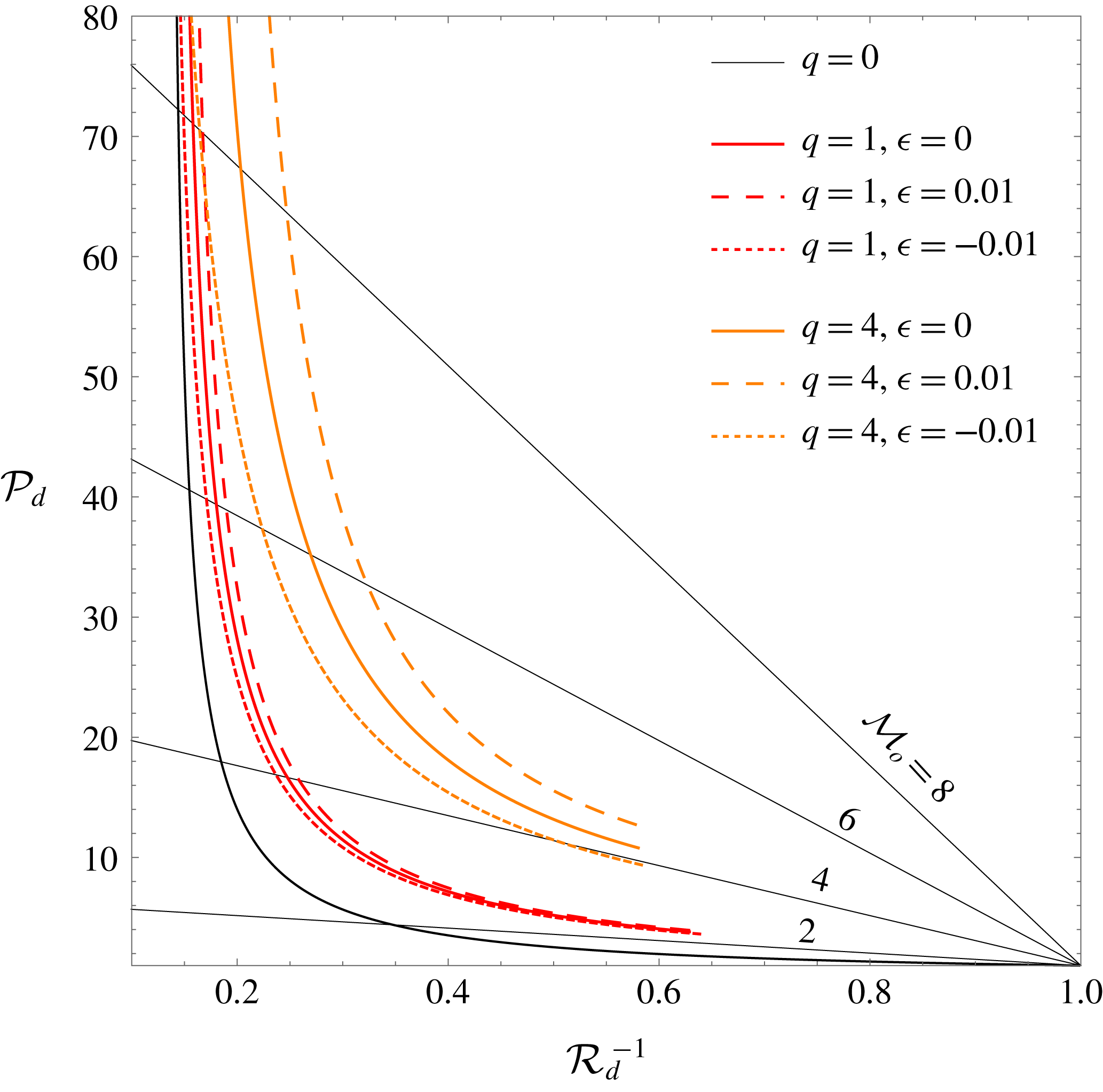
The RH curves are plotted in figure 1. The intersection of the (straight and thin) Rayleigh–Mickelson lines with the RH curves provides the final state after the detonation front. For sufficiently strong waves under constant-heat conditions, $\unicode[STIX]{x1D716}=0$ , the exothermic effect is negligible, and the corresponding curves approach the adiabatic RH curve. For $\unicode[STIX]{x1D716}\neq 0$ , however, as the energy released to the fluid particles scales with the shock strength squared, the effect is always noticeable for strong shocks. It is readily seen that positively correlated heat releases shift the curves upwards, whereas the opposite applies for negative values of $\unicode[STIX]{x1D716}$ . Although the shape of the curve is not significantly affected, this minor change induced by $\unicode[STIX]{x1D716}$ may have a pivotal impact on the perturbation dynamics, as will be shown in § 3.

Figure 1.

Rankine–Hugoniot curves for exothermic (coloured lines) and adiabatic (black line) shocks. Positive and negative correlations are represented by dashed and dotted lines, respectively. The straight narrow black lines are Rayleigh–Mickelson lines.

2.2 Linear perturbation analysis

Assuming that the background-flow variables are constant, which restricts the analysis to the stable detonation fronts commonly associated with overdriven detonations and/or low activation energies, regular perturbation analyses can be performed for the detonation front and the burnt-gas flow. Then, an initial ripple of the form $\unicode[STIX]{x1D713}_{d}(t=0)=\unicode[STIX]{x1D713}_{d0}\cos (k^{\prime }y^{\prime })$ is considered, where $\unicode[STIX]{x1D713}_{d0}$ is the initial amplitude and $k^{\prime }=2\unicode[STIX]{x03C0}/\unicode[STIX]{x1D706}$ is the associated wavenumber. 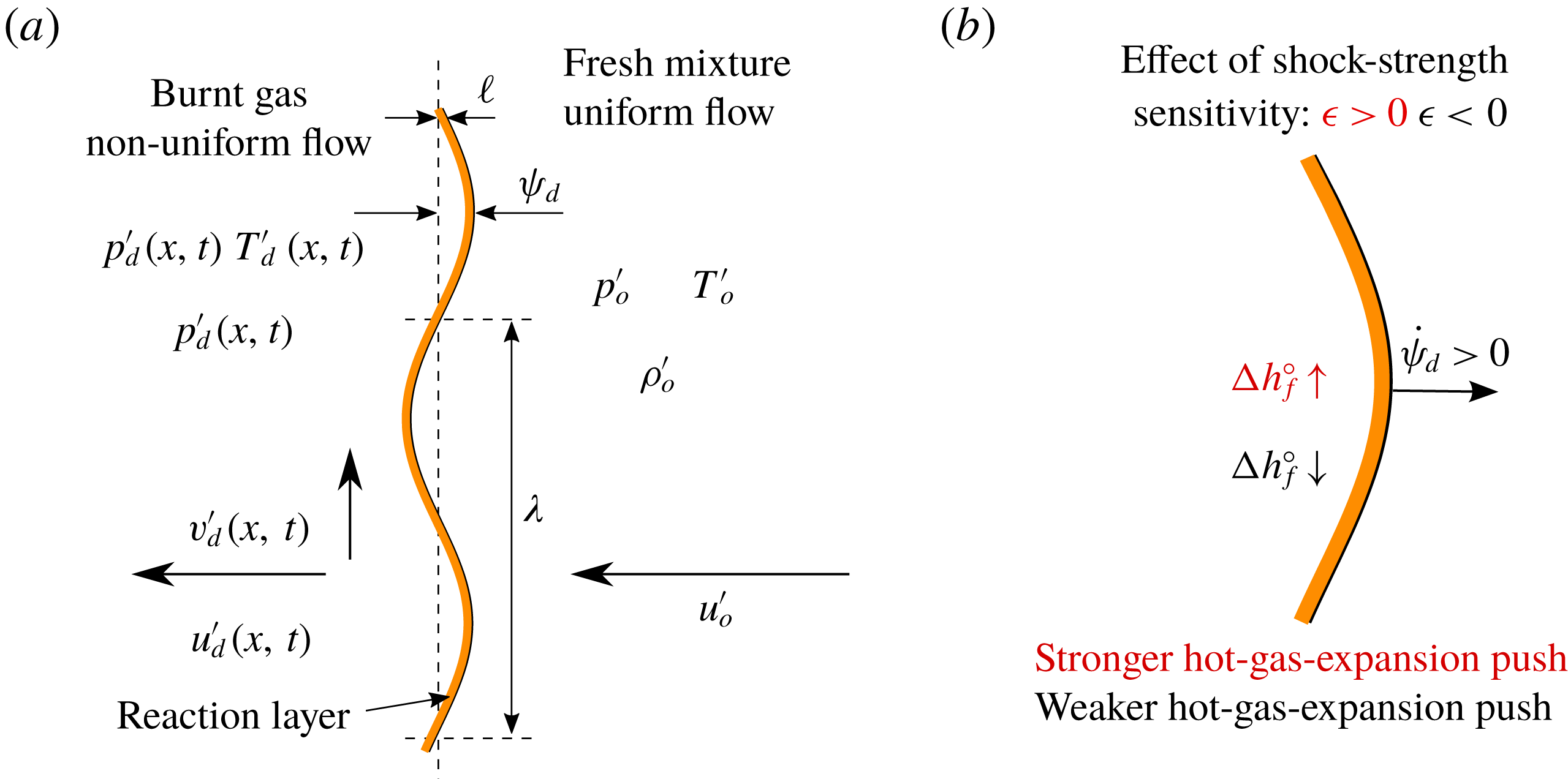Together with the stability prerequisite in the base-flow variables, linear theory and the fast-reaction-limit assumptions set the following limits on validity: $\ell \ll \unicode[STIX]{x1D713}_{d0}\ll \unicode[STIX]{x1D706}$ , with the corresponding lengths sketched in figure 2.

Figure 2.

Sketch of the corrugated detonation front and the representative lengths (a), with $\ell \ll \unicode[STIX]{x1D713}_{d0}\ll \unicode[STIX]{x1D706}$ . Qualitative description of the shock-strength sensitivity effect (b).

The wavenumber is employed to scale the spatial variables, $x=k^{\prime }x^{\prime }$ and $y=k^{\prime }y^{\prime }$ , and time is measured by the downstream speed of sound, $\unicode[STIX]{x1D70F}=a_{d}^{\prime }k^{\prime }t$ . The dimensionless order-of-unity detonation ripple is defined as $\unicode[STIX]{x1D709}_{d}=\unicode[STIX]{x1D713}_{d}/\unicode[STIX]{x1D713}_{d0}$ . The functions of interest are perturbed, and the small factor $\unicode[STIX]{x1D713}_{d0}k^{\prime }$ is used to scale the amplitude of the perturbations, namely,

(2.11a ) $$\begin{eqnarray}\displaystyle & \displaystyle p^{\prime }(x,y,\unicode[STIX]{x1D70F})=\unicode[STIX]{x1D70C}_{d}^{\prime }a_{d}^{\prime 2}[1+\unicode[STIX]{x1D713}_{d0}k^{\prime }\hat{p}(x,y,\unicode[STIX]{x1D70F})], & \displaystyle\end{eqnarray}$$

(2.11b ) $$\begin{eqnarray}\displaystyle & \displaystyle \unicode[STIX]{x1D70C}^{\prime }(x,y,\unicode[STIX]{x1D70F})=\unicode[STIX]{x1D70C}_{d}^{\prime }[1+\unicode[STIX]{x1D713}_{d0}k^{\prime }\hat{\unicode[STIX]{x1D70C}}(x,y,\unicode[STIX]{x1D70F})], & \displaystyle\end{eqnarray}$$

(2.11c ) $$\begin{eqnarray}\displaystyle & \displaystyle u^{\prime }(x,y,\unicode[STIX]{x1D70F})=a_{d}^{\prime }[1+\unicode[STIX]{x1D713}_{d0}k^{\prime }\hat{u} (x,y,\unicode[STIX]{x1D70F})], & \displaystyle\end{eqnarray}$$

(2.11d ) $$\begin{eqnarray}\displaystyle & \displaystyle v^{\prime }(x,y,\unicode[STIX]{x1D70F})=a_{d}^{\prime }[1+\unicode[STIX]{x1D713}_{d0}k^{\prime }\hat{v}(x,y,\unicode[STIX]{x1D70F})], & \displaystyle\end{eqnarray}$$

(2.12a ) $$\begin{eqnarray}\displaystyle & \displaystyle \frac{\unicode[STIX]{x2202}\hat{\unicode[STIX]{x1D70C}}}{\unicode[STIX]{x2202}\unicode[STIX]{x1D70F}}+\frac{\unicode[STIX]{x2202}\hat{u} }{\unicode[STIX]{x2202}x}+\hat{v}=0, & \displaystyle\end{eqnarray}$$

(2.12b ) $$\begin{eqnarray}\displaystyle & \displaystyle \frac{\unicode[STIX]{x2202}\hat{u} }{\unicode[STIX]{x2202}\unicode[STIX]{x1D70F}}+\frac{\unicode[STIX]{x2202}\hat{p}}{\unicode[STIX]{x2202}x}=0, & \displaystyle\end{eqnarray}$$

(2.12c ) $$\begin{eqnarray}\displaystyle & \displaystyle \frac{\unicode[STIX]{x2202}\hat{v}}{\unicode[STIX]{x2202}\unicode[STIX]{x1D70F}}-\hat{p}=0, & \displaystyle\end{eqnarray}$$

(2.12d ) $$\begin{eqnarray}\displaystyle & \displaystyle \frac{\unicode[STIX]{x2202}\hat{p}}{\unicode[STIX]{x2202}\unicode[STIX]{x1D70F}}-\frac{\unicode[STIX]{x2202}\hat{\unicode[STIX]{x1D70C}}}{\unicode[STIX]{x2202}\unicode[STIX]{x1D70F}}=0, & \displaystyle\end{eqnarray}$$

$x$

$y$

$\hat{p}$

$\hat{v}$

$\cos (y)$

$\sin (y)$

(2.13) $$\begin{eqnarray}\frac{\unicode[STIX]{x2202}^{2}\hat{p}}{\unicode[STIX]{x2202}\unicode[STIX]{x1D70F}^{2}}=\frac{\unicode[STIX]{x2202}^{2}\hat{p}}{\unicode[STIX]{x2202}x^{2}}-\hat{p}.\end{eqnarray}$$

Figure 3.

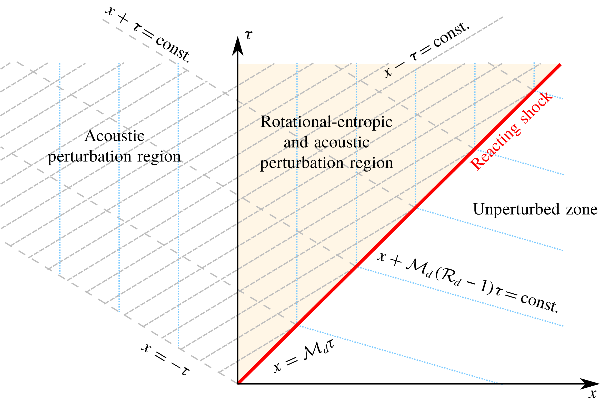
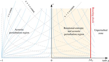
Integration domain and distinguished regions. Blue dotted lines refer to the particle paths, grey dashed lines indicate the positive and negative characteristic paths, respectively, and the red solid line defines the detonation trajectory.

The problem reduces to that of integrating the linearized Euler equations or, equivalently, the wave equation (2.13) for $\unicode[STIX]{x1D70F}\geqslant 0$ over the domain delimited by the leading reflected sonic wave travelling backwards, $x=-\unicode[STIX]{x1D70F}$ , and the reaction front moving forwards, $x={\mathcal{M}}_{d}\unicode[STIX]{x1D70F}$ , as sketched in figure 3. One boundary condition is provided by the isolation assumption, which translates into neglect of the effect of the acoustic waves reaching the detonation from behind; this is detailed mathematically in the discussion after (A 7) in appendix A. Note that this condition does not restrict the existence of right-travelling waves in the burnt gas, i.e. waves propagating in the detonation propagation direction, but it impedes their ability to reach the detonation front from behind because they are all generated at the detonation front and there is no reflecting boundary downstream. The other boundary condition is given by the flow properties at the detonation front,

(2.14) $$\begin{eqnarray}\frac{\hat{p}(x={\mathcal{M}}_{d}\unicode[STIX]{x1D70F})}{\hat{p}_{d}}=\frac{\hat{\unicode[STIX]{x1D70C}}(x={\mathcal{M}}_{d}\unicode[STIX]{x1D70F})}{\hat{\unicode[STIX]{x1D70C}}_{d}}=\frac{\hat{u} (x={\mathcal{M}}_{d}\unicode[STIX]{x1D70F})}{\hat{u} _{d}}=\frac{\hat{v}(x={\mathcal{M}}_{d}\unicode[STIX]{x1D70F})}{\hat{v}_{d}}=1,\end{eqnarray}$$

for the pressure, density and velocity perturbations, respectively, which are given by the linearized reactive RH equations, namely,

(2.15a ) $$\begin{eqnarray}\displaystyle & \displaystyle \frac{\text{d}\unicode[STIX]{x1D709}_{d}}{\text{d}\unicode[STIX]{x1D70F}}(\unicode[STIX]{x1D70F})={\displaystyle \frac{{\mathcal{R}}_{d}}{{\mathcal{R}}_{d}-1}}{\displaystyle \frac{1-\unicode[STIX]{x1D6E4}_{d}}{2{\mathcal{M}}_{d}}}\hat{p}_{d}(\unicode[STIX]{x1D70F}), & \displaystyle\end{eqnarray}$$

(2.15b ) $$\begin{eqnarray}\displaystyle & \displaystyle \hat{u} _{d}(\unicode[STIX]{x1D70F})={\displaystyle \frac{1+\unicode[STIX]{x1D6E4}_{d}}{2{\mathcal{M}}_{d}}}\hat{p}_{d}(\unicode[STIX]{x1D70F}), & \displaystyle\end{eqnarray}$$

(2.15c ) $$\begin{eqnarray}\displaystyle & \displaystyle \hat{\unicode[STIX]{x1D70C}}_{d}(\unicode[STIX]{x1D70F})={\displaystyle \frac{\unicode[STIX]{x1D6E4}_{d}}{{\mathcal{M}}_{d}^{2}}}\hat{p}_{d}(\unicode[STIX]{x1D70F}), & \displaystyle\end{eqnarray}$$

(2.15d ) $$\begin{eqnarray}\displaystyle & \displaystyle \hat{v}_{d}(\unicode[STIX]{x1D70F})={\mathcal{M}}_{d}({\mathcal{R}}_{d}-1){\displaystyle \frac{\unicode[STIX]{x2202}\unicode[STIX]{x1D709}_{d}}{\unicode[STIX]{x2202}y}}(\unicode[STIX]{x1D70F}). & \displaystyle\end{eqnarray}$$

Note that, unlike the one-dimensional RH equations, the detonation ripple function, which is to be determined, calls for an extra independent equation: the momentum conservation equation in the transverse direction, which ultimately translates into the conservation of the tangential velocity.

The mass compression factor ${\mathcal{R}}_{d}$ and the post-detonation Mach number ${\mathcal{M}}_{d}$ are given in (2.5) and (2.7) as functions of the gas polytropic index $\unicode[STIX]{x1D6FE}$ , the upstream Mach number ${\mathcal{M}}_{o}$ and the non-adiabatic contribution ${\mathcal{H}}_{0}$ . The factor that accounts for the RH slope downstream, (1.2), which is found to govern the stability of the reactive shock, is

(2.16) $$\begin{eqnarray}\unicode[STIX]{x1D6E4}_{d}=u_{d}^{\prime 2}\left({\displaystyle \frac{\unicode[STIX]{x2202}p_{d}^{\prime }}{\unicode[STIX]{x2202}\unicode[STIX]{x1D70C}_{d}^{\prime }}}\right)^{-1}={\displaystyle \frac{\unicode[STIX]{x1D6FE}{\mathcal{M}}_{o}^{2}}{{\mathcal{R}}_{d}^{2}}}\left({\displaystyle \frac{\unicode[STIX]{x2202}{\mathcal{P}}_{d}}{\unicode[STIX]{x2202}{\mathcal{R}}_{d}}}\right)^{-1},\end{eqnarray}$$

and relates to the so-called DK parameter through $h=-\unicode[STIX]{x1D6E4}_{d}$ (see D’Yakov Reference D’Yakov1954; Kontorovich Reference Kontorovich1957). It is readily seen that this factor tends to ${\mathcal{M}}_{o}^{-2}$ in the adiabatic limit, $q\ll 1$ , to yield a perfect-gas equation of state.

Manipulation of the linearized RH equations leads to the following system of equations for the detonation boundary conditions:

(2.17) $$\begin{eqnarray}{\displaystyle \frac{\text{d}\unicode[STIX]{x1D709}_{d}}{\text{d}\unicode[STIX]{x1D70F}}}=\unicode[STIX]{x1D70E}_{a}\hat{p}_{d}\end{eqnarray}$$

and

(2.18) $$\begin{eqnarray}(\unicode[STIX]{x1D70E}_{b}+{\mathcal{M}}_{d})\frac{\unicode[STIX]{x2202}\hat{p}_{d}}{\unicode[STIX]{x2202}\unicode[STIX]{x1D70F}}+(\unicode[STIX]{x1D70E}_{b}{\mathcal{M}}_{d}+1)\left.\frac{\unicode[STIX]{x2202}\hat{p}}{\unicode[STIX]{x2202}x}\right|_{x={\mathcal{M}}_{d}\unicode[STIX]{x1D70F}}=-{\mathcal{M}}_{d}^{2}({\mathcal{R}}_{d}-1)\unicode[STIX]{x1D709}_{d},\end{eqnarray}$$

to be employed when integrating the Euler equations for the burnt gas. The factors accompanying the pressure perturbation in (2.17) and (2.18) are conveniently expressed it terms of the functions

(2.19a,b ) $$\begin{eqnarray}\unicode[STIX]{x1D70E}_{a}={\displaystyle \frac{{\mathcal{R}}_{d}}{{\mathcal{R}}_{d}-1}}{\displaystyle \frac{1-\unicode[STIX]{x1D6E4}_{d}}{2{\mathcal{M}}_{d}}}\quad \text{and}\quad \unicode[STIX]{x1D70E}_{b}={\displaystyle \frac{1+\unicode[STIX]{x1D6E4}_{d}}{2{\mathcal{M}}_{d}}}.\end{eqnarray}$$

3.1 General asymptotic theory

The qualitative response of the detonation front can be inferred with the aid of figure 2, where the shock-strength dependence of the heat released is depicted for positive and negative values of $\unicode[STIX]{x1D716}$ . Positive correlations with the shock strength, which, in the linear regime, scales with the growth of the detonation shape as $\unicode[STIX]{x1D6FF}{\mathcal{M}}_{o}=\dot{\unicode[STIX]{x1D709}}_{d}{\mathcal{M}}_{o}/({\mathcal{R}}_{d}{\mathcal{M}}_{d})$ , translate into amplified expansion of the hot products within the reaction zone when the detonation accelerates, $\dot{\unicode[STIX]{x1D709}}_{d}>0$ , and a diminished expansion-driven push when it decelerates, $\dot{\unicode[STIX]{x1D709}}_{d}<0$ . Generally, for very small values of $\unicode[STIX]{x1D716}$ , this positive feedback decreases the damping of the oscillation amplitude towards a planar shape. It is shown later that, for sufficiently large values of $\unicode[STIX]{x1D716}$ , yet still much smaller than unity, $\unicode[STIX]{x1D716}\sim {\mathcal{M}}_{o}^{-2}\ll 1$ , the detonation oscillates with constant amplitude in the long term. This positive feedback that heat release may exert on the detonation dynamics resembles the Rayleigh criterion for the thermoacoustic instability. The opposite case, $\unicode[STIX]{x1D716}<0$ , has a stabilizing counter-effect, with the endothermic perturbation decreasing the detonation ripple’s growth, thereby promoting faster decay towards the final planar shape.

The quantitative response that sets the limits of the distinguished asymptotic regimes is less straightforward. For the detonation to spontaneously and constantly radiate acoustic waves downstream, two conditions must be fulfilled simultaneously: the reactive shock must oscillate with a non-decaying amplitude, and the frequency of the oscillations must be sufficiently high. The latter condition is equivalent to saying that the acoustic wavenumber vector in the detonation reference frame points backwards. This condition is easily deduced by anticipating that sonic waves travelling in the burnt-gas region are functions of $(\unicode[STIX]{x1D701}_{a}\unicode[STIX]{x1D70F}-k_{a}x)$ . The dimensionless frequency $\unicode[STIX]{x1D701}_{a}$ and wavenumber $k_{a}$ are obtained from the adiabatic dispersion relation $\unicode[STIX]{x1D701}_{a}^{2}=k_{a}^{2}+1$ , as derived from (2.13), along with the compatibility condition at the reaction front, $\unicode[STIX]{x1D714}=\unicode[STIX]{x1D701}_{a}-{\mathcal{M}}_{d}k_{a}$ , which provides

(3.1) $$\begin{eqnarray}k_{a}=\frac{\unicode[STIX]{x1D714}{\mathcal{M}}_{d}-\sqrt{\unicode[STIX]{x1D714}^{2}-1+{\mathcal{M}}_{d}^{2}}}{1-{\mathcal{M}}_{d}^{2}}\end{eqnarray}$$

and

(3.2) $$\begin{eqnarray}\unicode[STIX]{x1D701}_{a}=\frac{\unicode[STIX]{x1D714}-{\mathcal{M}}_{d}\sqrt{\unicode[STIX]{x1D714}^{2}-1+{\mathcal{M}}_{d}^{2}}}{1-{\mathcal{M}}_{d}^{2}}.\end{eqnarray}$$

Acoustic perturbations become evanescent when the radicand in (3.1) and (3.2) becomes negative, i.e. when the detonation frequency satisfies $\unicode[STIX]{x1D714}<\sqrt{1-{\mathcal{M}}_{d}^{2}}$ . In contrast, constant-amplitude waves occur when $\unicode[STIX]{x1D714}\geqslant \sqrt{1-{\mathcal{M}}_{d}^{2}}$ , with the sign of $k_{a}$ determining the propagation direction of the travelling waves. Positive values of $k_{a}$ , or $\sqrt{1-{\mathcal{M}}_{d}^{2}}<\unicode[STIX]{x1D714}<1$ , refer to waves travelling to the right, whereas the opposite describes waves travelling to the left, $\unicode[STIX]{x1D714}>1$ . Then, the singular case $\unicode[STIX]{x1D714}=1$ corresponds to standing acoustic waves in the longitudinal direction.

The Laplace transforms of the detonation ripple and pressure disturbances, given in (A 10) and (A 11), respectively, provide the following dispersion relationship:

(3.3) $$\begin{eqnarray}s\sqrt{s^{2}+1}+\unicode[STIX]{x1D70E}_{b}s^{2}+\unicode[STIX]{x1D70E}_{c}=0,\end{eqnarray}$$

with the nature of the poles describing the long-term response (Clavin & Williams Reference Clavin and Williams2012; Clavin & Searby Reference Clavin and Searby2016).

The value of $\unicode[STIX]{x1D70E}_{b}$ relative to $\unicode[STIX]{x1D70E}_{c}$ , which is shown in (A 12), defines the distinguished limits. The acoustic nature of the burnt-gas perturbation field is responsible for the term $\sqrt{s^{2}+1}$ in (3.3), which introduces a branch cut in the complex plane of the Laplace variable $s$ . As a direct consequence, not all purely imaginary poles that are roots of this equation are translated into undamped oscillations on the long time scale (Clavin & Searby Reference Clavin and Searby2016).

The condition that sets the limits for stable oscillations is $s=\pm \text{i}$ , which occurs when $\unicode[STIX]{x1D70E}_{b}=\unicode[STIX]{x1D70E}_{c}$ , as easily verified from (3.3). The dispersion relation is then recast as $\sqrt{s^{2}+1}(s+\unicode[STIX]{x1D70E}_{b}\sqrt{s^{2}+1})=0$ , which, in the temporal domain, translates into damped oscillations whose asymptotic decay rate is proportional to $\unicode[STIX]{x1D70F}^{-1/2}$ . For adiabatic shocks in perfect gases, this singular condition is only met in the strong-shock limit (Fraley Reference Fraley1986). Permanent oscillations at the reaction front occur when $\unicode[STIX]{x1D70E}_{b}<\unicode[STIX]{x1D70E}_{c}$ , that is, when the imaginary poles in (3.3) lie outside the branch cut. The asymptotic detonation-oscillation frequency is $\unicode[STIX]{x1D714}=\unicode[STIX]{x1D701}_{-}\sqrt{1-{\mathcal{M}}_{d}^{2}}$ , where

(3.4) $$\begin{eqnarray}\unicode[STIX]{x1D701}_{\pm }^{2}={\displaystyle \frac{2\unicode[STIX]{x1D70E}_{b}\unicode[STIX]{x1D70E}_{c}-1}{2(\unicode[STIX]{x1D70E}_{b}^{2}-1)}}\left[1\pm {\displaystyle \frac{\sqrt{4\unicode[STIX]{x1D70E}_{c}(\unicode[STIX]{x1D70E}_{c}-\unicode[STIX]{x1D70E}_{b})+1}}{2\unicode[STIX]{x1D70E}_{b}\unicode[STIX]{x1D70E}_{c}-1}}\right]\end{eqnarray}$$

tends to unity in the limit $\unicode[STIX]{x1D70E}_{b}-\unicode[STIX]{x1D70E}_{c}\ll 1$ .

The DK stability limit depends on the local slope of the RH curve in the burnt-gas state, as noted in § 1. This is commonly presented as a function of the parameter

(3.5) $$\begin{eqnarray}\unicode[STIX]{x1D711}_{rad}={\displaystyle \frac{{\mathcal{M}}_{d}^{2}({\mathcal{R}}_{d}+1)-1}{{\mathcal{M}}_{d}^{2}({\mathcal{R}}_{d}-1)+1}},\end{eqnarray}$$

which separates the acoustically radiating regime from the non-radiating regime. The equation $\unicode[STIX]{x1D6E4}_{d}=\unicode[STIX]{x1D711}_{rad}$ is equivalent to $\unicode[STIX]{x1D70E}_{b}=\unicode[STIX]{x1D70E}_{c}$ , which is derived above.

When $\unicode[STIX]{x1D70E}_{b}>\unicode[STIX]{x1D70E}_{c}$ , the detonation front oscillates towards the asymptotic planar solution with an amplitude that decays in time in accordance with the power law $\unicode[STIX]{x1D70F}^{-3/2}$ . However, two distinguished scenarios exist: when $\unicode[STIX]{x1D70E}_{b}>\unicode[STIX]{x1D70E}_{c}+1/(4\unicode[STIX]{x1D70E}_{c})$ (or $\unicode[STIX]{x1D6EC}<0$ , as defined in Bates (Reference Bates2004)), the approach towards the asymptotic decay rate occurs faster than it does under regular conditions, namely, $\unicode[STIX]{x1D70E}_{c}+1/(4\unicode[STIX]{x1D70E}_{c})>\unicode[STIX]{x1D70E}_{b}>\unicode[STIX]{x1D70E}_{c}$ . Regular conditions are associated with finite-strength shocks moving adiabatically in perfect gases. The limit that distinguishes fast or regular damping can also be expressed as $\unicode[STIX]{x1D6E4}_{d}=\unicode[STIX]{x1D711}_{dam}$ , where

(3.6) $$\begin{eqnarray}\unicode[STIX]{x1D711}_{dam}={\displaystyle \frac{{\mathcal{R}}_{d}{\mathcal{M}}_{d}^{2}-(1-{\mathcal{M}}_{d}^{2})^{3/2}\sqrt{1-{\mathcal{R}}_{d}^{-1}}}{{\mathcal{R}}_{d}{\mathcal{M}}_{d}^{2}+1-{\mathcal{M}}_{d}^{2}}}.\end{eqnarray}$$

A supersonic front becomes unstable when $\unicode[STIX]{x1D6E4}_{d}<-(1+2{\mathcal{M}}_{d})$ or $\unicode[STIX]{x1D70E}_{b}<-1$ . For this condition to be met, the RH slope must reverse, which does not occur in detonations moving through perfect gases. 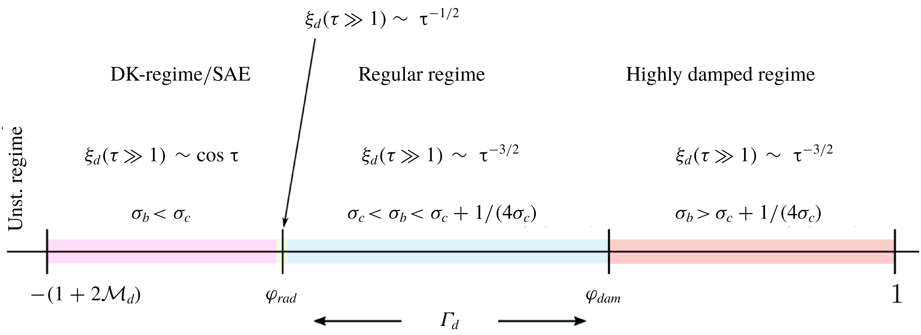Within the parametric domain that defines strength-sensitive detonation, ${\mathcal{M}}_{o}\sim \sqrt{q}$ , $q\sim 1{-}10$ , and $|\unicode[STIX]{x1D716}|\ll 1$ , four regimes are identified and delimited in figure 4. The colour code used here is the same as that used in the computations of the asymptotic temporal evolution in figure 9.

Figure 4.

General stability limits for detonation waves (Clavin & Williams Reference Clavin and Williams2012; Clavin & Searby Reference Clavin and Searby2016).

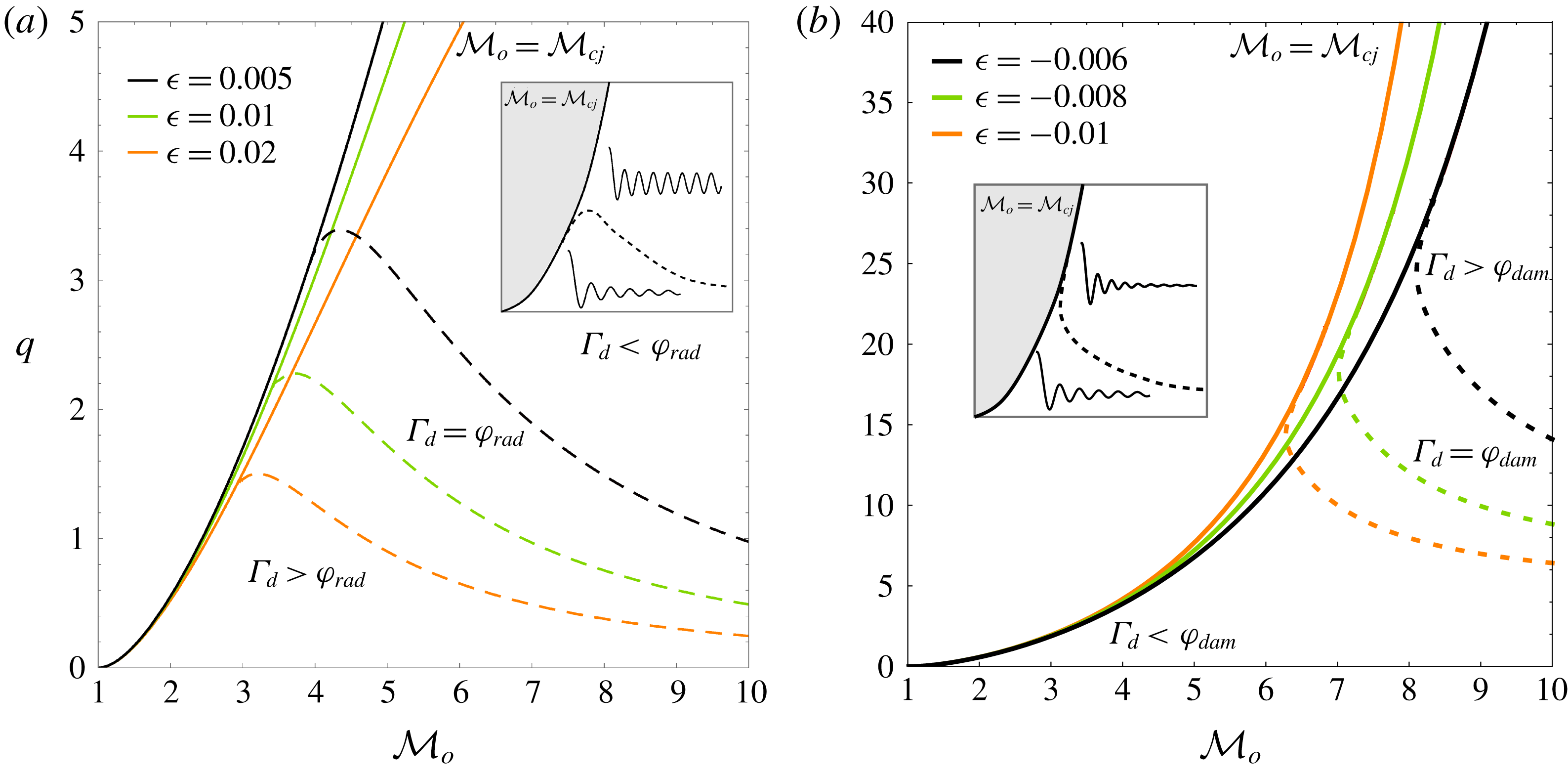
The above-mentioned parameters are computed in figure 5 for $\unicode[STIX]{x1D716}>0$ (a) and $\unicode[STIX]{x1D716}<0$ (b) as functions of ${\mathcal{M}}_{o}$ and $q$ . Solid lines correspond to ${\mathcal{M}}_{o}={\mathcal{M}}_{cj}$ , dashed lines to the limit $\unicode[STIX]{x1D6E4}_{d}=\unicode[STIX]{x1D711}_{rad}$ and dotted lines to $\unicode[STIX]{x1D6E4}_{d}=\unicode[STIX]{x1D711}_{dam}$ . The region above the solid lines is discarded because it corresponds to ${\mathcal{M}}_{o}<{\mathcal{M}}_{cj}$ . The region below the dashed/dotted lines corresponds to the regular oscillating regime, which is similar to that found in adiabatic shock waves. It is found that only positively correlated shock-strength sensitivities ( $\unicode[STIX]{x1D716}>0$ ) lead to constant-amplitude oscillations, which correspond to the region enclosed by the lines ${\mathcal{M}}_{o}={\mathcal{M}}_{cj}$ and $\unicode[STIX]{x1D6E4}_{d}=\unicode[STIX]{x1D711}_{rad}$ . In contrast, strongly damped oscillations are restricted to negative shock-strength sensitivities ( $\unicode[STIX]{x1D716}<0$ ), with the region bounded by the curves ${\mathcal{M}}_{o}={\mathcal{M}}_{cj}$ and $\unicode[STIX]{x1D6E4}_{d}=\unicode[STIX]{x1D711}_{dam}$ being the parameter space associated with this regime. For positively correlated shock-strength sensitivities (figure 5 a), it is found that the point of detachment occurs before order-of-unity energy variations, as observed for $\unicode[STIX]{x1D716}=0.005$ and ${\mathcal{M}}_{o}\sim 4$ , which corresponds to energy changes of less than 10 % of the global heat released. For sufficiently weak detonations, the energy change induced by the shock strength is negligible; therefore, the curves $\unicode[STIX]{x1D6E4}_{d}=\unicode[STIX]{x1D711}_{rad}$ and $\unicode[STIX]{x1D6E4}_{d}=\unicode[STIX]{x1D711}_{dam}$ approach the boundary ${\mathcal{M}}_{o}={\mathcal{M}}_{cj}$ . For finite shock strengths, however, the shock-strength sensitivity is no longer negligible, and the curves detach from their respective boundaries, enabling the possibility of permanent and strongly damped oscillation regimes for $\unicode[STIX]{x1D716}>0$ and $\unicode[STIX]{x1D716}<0$ , respectively. For negatively correlated cases, the shock strength needed to switch to strongly damped oscillations is higher, making this condition harder to meet. Results agree with previous analysis developed for stable detonations, i.e. characterized by a sufficiently low activation energy, in the long-wavelength limit (Bourlioux et al. Reference Bourlioux, Majda and Royburd1992; Clavin & Williams Reference Clavin and Williams2012; Clavin & Searby Reference Clavin and Searby2016).

Figure 5.

Dynamic detonation regimes for positively (a) and negatively (b) correlated shock-strength sensitivities as functions of ${\mathcal{M}}_{o}$ and $q$ . Solid lines correspond to values of ${\mathcal{M}}_{o}={\mathcal{M}}_{cj}$ . The curves have been computed with $\unicode[STIX]{x1D6FE}=1.3$ .

The foregoing stability limits could have been obtained omitting the previous analysis on the poles in the complex plane. Direct inspection of (1.1) and (1.3) presented in the introduction, with the function $\unicode[STIX]{x1D6E4}_{d}$ being already given in (2.16) and (2.10), provides the stability limits of the planar reacting front. Besides, previous works have been devoted to investigate the stability limits of planar reactive shocks and they offer a comprehensive and exhaustive analysis on the topic, including the extension to nonlinear perturbations (Majda & Rosales Reference Majda and Rosales1983; Clavin & Searby Reference Clavin and Searby2016). It is, however, convenient to repeat them here in the terms presented above, since part of the analysis is useful to describe the transient evolution of the reactive front and the properties of the burnt-gas variables. Moreover, the position of the poles in the complex plane is paramount to determine the perturbation decay rates and to obtain the corresponding strongly and weakly overdriven limits addressed below.

3.2 Strongly and weakly overdriven detonation limits for $\unicode[STIX]{x1D6E4}_{d}=\unicode[STIX]{x1D711}_{rad}$

The transition to acoustically radiating detonations can be investigated in the limits of strongly, ${\mathcal{M}}_{o}/{\mathcal{M}}_{cj}\gg 1$ , and weakly, ${\mathcal{M}}_{o}/{\mathcal{M}}_{cj}-1\ll 1$ , overdriven detonations. As inferred from figure 5(a), the iso-curve $\unicode[STIX]{x1D6E4}_{d}=\unicode[STIX]{x1D711}_{rad}$ shows that the value of $q$ required to switch to the oscillatory mode decreases when the Mach number is sufficiently large and increases.

Performing a regular expansion for large Mach numbers, ${\mathcal{M}}_{o}/{\mathcal{M}}_{cj}\gg 1$ , and small sensitivity parameters, $\unicode[STIX]{x1D716}\ll 1$ , yields the following expression for the iso-curve $\unicode[STIX]{x1D6E4}_{d}=\unicode[STIX]{x1D711}_{rad}$ :

(3.7) $$\begin{eqnarray}{\mathcal{M}}_{o}^{2}={\displaystyle \frac{1-2q\unicode[STIX]{x1D716}(2+3q)+(1-2q\unicode[STIX]{x1D716})\sqrt{1-4q\unicode[STIX]{x1D716}}}{2q\unicode[STIX]{x1D716}\sqrt{1-4q\unicode[STIX]{x1D716}}\left(1+\sqrt{1-4q\unicode[STIX]{x1D716}}\right)}}\sim {\displaystyle \frac{1}{2q\unicode[STIX]{x1D716}}}-(1+q)-\unicode[STIX]{x1D716}q(2+3q)+O(\unicode[STIX]{x1D716}^{2}),\end{eqnarray}$$

which shows that the limiting Mach number increases as $q$ and $\unicode[STIX]{x1D716}$ decrease. It is also found that the curve $\unicode[STIX]{x1D6E4}_{d}=\unicode[STIX]{x1D711}_{rad}$ approaches the asymptote $q=0$ for any $\unicode[STIX]{x1D716}>0$ . For the singular case of $\unicode[STIX]{x1D716}=0$ , the condition $\unicode[STIX]{x1D6E4}_{d}=\unicode[STIX]{x1D711}_{rad}$ is only met for ${\mathcal{M}}_{o}\gg 1$ , as found for adiabatic shocks in the strong-shock limit (Fraley Reference Fraley1986), which leaves no room for stable oscillations.

Weakly overdriven conditions are evaluated by the functions $\unicode[STIX]{x1D70E}_{b}$ and $\unicode[STIX]{x1D70E}_{c}$ . Regular expansions in the limit ${\mathcal{M}}_{o}/{\mathcal{M}}_{cj}-1\ll 1$ reveal that $\unicode[STIX]{x1D70E}_{b}$ approaches unity in the form $1+O(\sqrt{{\mathcal{M}}_{o}/{\mathcal{M}}_{cj}-1})$ , whereas the function $\unicode[STIX]{x1D70E}_{c}$ converges to a finite value $\unicode[STIX]{x1D70E}_{c}^{\ast }+O(\sqrt{{\mathcal{M}}_{o}/{\mathcal{M}}_{cj}-1})$ , where

(3.8) $$\begin{eqnarray}\unicode[STIX]{x1D70E}_{c}^{\ast }=\unicode[STIX]{x1D70E}_{c}({\mathcal{M}}_{o}={\mathcal{M}}_{cj})={\displaystyle \frac{\sqrt{1+q+\unicode[STIX]{x1D716}}+(1+2\unicode[STIX]{x1D716})\sqrt{q}}{2(1-4q\unicode[STIX]{x1D716})\sqrt{1+q+\unicode[STIX]{x1D716}}}}.\end{eqnarray}$$

The limiting condition that separates stable and decaying oscillations $\unicode[STIX]{x1D70E}_{b}=\unicode[STIX]{x1D70E}_{c}$ provides

(3.9) $$\begin{eqnarray}q={\displaystyle \frac{\sqrt{1+\unicode[STIX]{x1D716}}}{8\unicode[STIX]{x1D716}\sqrt{1+\unicode[STIX]{x1D716}}+4(1+2\unicode[STIX]{x1D716})\sqrt{\unicode[STIX]{x1D716}}}}\sim \frac{1}{4\sqrt{\unicode[STIX]{x1D716}}}-{\displaystyle \frac{1}{2}}+{\displaystyle \frac{5\sqrt{\unicode[STIX]{x1D716}}}{8}}-{\displaystyle \frac{\unicode[STIX]{x1D716}}{2}}+O(\unicode[STIX]{x1D716}^{3/2}),\end{eqnarray}$$

as the value above which the reacting shock undergoes stable oscillations in the CJ regime. As before, the small sensitivity parameter in (3.9) appears as a singularity in the leading-order term. Then, for reactive shocks whose sensitivity to the heat released is strictly null, $\unicode[STIX]{x1D716}=0$ , the oscillatory mode is infeasible.

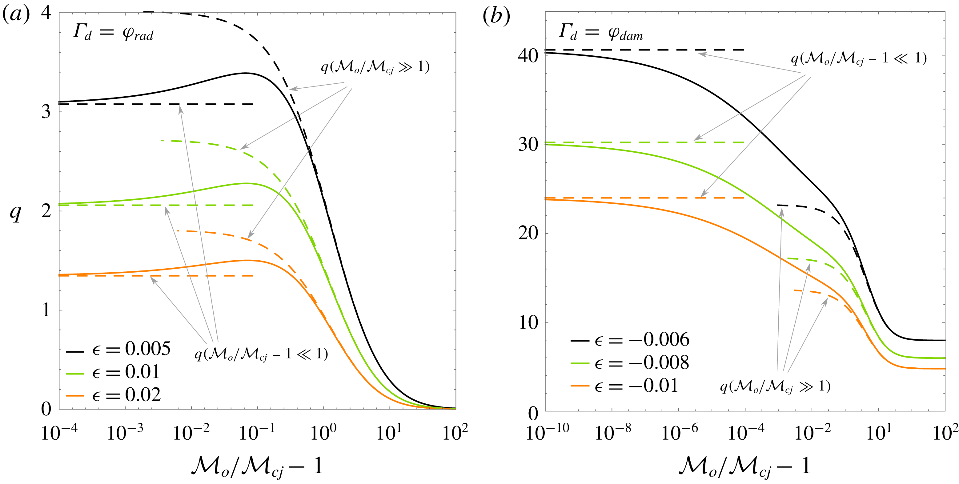
The strongly and weakly overdriven limits, which are found to be independent of the adiabatic index $\unicode[STIX]{x1D6FE}$ , are computed in figure 6(a) as a function of ${\mathcal{M}}_{o}/{\mathcal{M}}_{cj}-1$ for the conditions in figure 5(a). Figure 6(a) shows that weakly overdriven detonations call for a minimum amount of heat to be released to achieve the stable oscillatory mode; this critical value is inversely proportional to $\sqrt{\unicode[STIX]{x1D716}}$ . Similarly, strongly overdriven detonations have critical Mach numbers that are inversely proportional to $\unicode[STIX]{x1D716}$ .

3.3 Strongly and weakly overdriven detonation limits for $\unicode[STIX]{x1D6E4}_{d}=\unicode[STIX]{x1D711}_{dam}$

The strongly overdriven limit ${\mathcal{M}}_{o}/{\mathcal{M}}_{cj}\gg 1$ corresponding to the condition $\unicode[STIX]{x1D6E4}_{d}=\unicode[STIX]{x1D711}_{dam}$ is

(3.10) $$\begin{eqnarray}{\mathcal{M}}_{o}^{2}\sim {\displaystyle \frac{2}{3}}{\displaystyle \frac{2\unicode[STIX]{x1D6FE}-1-2\unicode[STIX]{x1D6FE}^{1/3}(1+3q)+\unicode[STIX]{x1D6FE}^{2/3}(1+4q)}{\unicode[STIX]{x1D6FE}^{1/3}(4q\unicode[STIX]{x1D716}+\unicode[STIX]{x1D6FE}^{2/3}-1)}}+O(\unicode[STIX]{x1D716}^{1/2})\end{eqnarray}$$

to leading order, which presents a pole at $q=(1-\unicode[STIX]{x1D6FE}^{2/3})/(4\unicode[STIX]{x1D716})$ . Unlike the radiating condition shown in (3.7), the iso-curve $\unicode[STIX]{x1D6E4}_{d}=\unicode[STIX]{x1D711}_{dam}$ approaches a constant corresponding to the minimum heat of reaction needed to enter the strongly damped oscillation regime.

Figure 6.

Weakly and strongly overdriven limits for $\unicode[STIX]{x1D6E4}_{d}=\unicode[STIX]{x1D711}_{rad}$ and  $\unicode[STIX]{x1D6E4}_{d}=\unicode[STIX]{x1D711}_{dam}$ for $\unicode[STIX]{x1D6FE}=1.3$ .

The opposite weakly overdriven limit for low sensitivities is

(3.11) $$\begin{eqnarray}q\sim -\left({\displaystyle \frac{1}{4\unicode[STIX]{x1D716}}}+1+\unicode[STIX]{x1D716}\right)+O(\unicode[STIX]{x1D716}^{2}),\end{eqnarray}$$

provided that $1=\unicode[STIX]{x1D70E}_{c}^{\ast }+1/(4\unicode[STIX]{x1D70E}_{c}^{\ast })$ in the CJ regime, with $\unicode[STIX]{x1D70E}_{c}^{\ast }$ being given in (3.8). Because $\unicode[STIX]{x1D6E4}_{d}=\unicode[STIX]{x1D711}_{dam}$ is a monotonically decreasing function of ${\mathcal{M}}_{o}/{\mathcal{M}}_{cj}-1$ , any amount of dimensionless heat released greater than that in (3.11) makes the detonation oscillations attenuate quickly. Unlike the value obtained in (3.9), the factor $q\sim 1/\unicode[STIX]{x1D716}$ , which demands that much more heat be released to reach the strongly damped regime under CJ conditions.

Both limits are computed in figure 6(b) for the conditions in figure 5(b). It is found that small deviations in the overdrive with respect to the CJ regime quickly decrease the critical heat release required to enter the strongly damped oscillatory mode. Convergence to the limiting value (3.11) is very slow. When ${\mathcal{M}}_{o}={\mathcal{M}}_{cj}$ , linear perturbation theory in the fast-reaction limit predicts that $\unicode[STIX]{x1D6E4}_{d}=\unicode[STIX]{x1D711}_{rad}$ is unconditionally satisfied for any value of $q$ , which makes the front oscillations decay with $\unicode[STIX]{x1D70F}^{-1/2}$ .

Note that the case ${\mathcal{M}}_{o}={\mathcal{M}}_{cj}$ is singular, i.e. any positive deviation of the velocity field with respect to the base flow may generate a locally supersonic zone, and the same applies to negative temperature perturbations. In principle, the detonation travelling is restricted to an asymmetric propagation condition: the detonation can move faster than the CJ velocity but not slower. When analysed in the strong-shock limit, both post-detonation gas velocity and hot-gas speed of sound scale linearly with the shock intensity, $u_{d,cj}\sim a_{d,cj}\sim u_{o,cj}\unicode[STIX]{x1D6FE}/(\unicode[STIX]{x1D6FE}-1)$ , thereby allowing both positive and negative small variations of the propagating velocity, with the governing constraint on the sonic condition downstream ( $M_{d}=1$ ) unaltered. However, this adds a restriction to the perturbation amplitudes in the weakly overdriven limit, as the reacting flow cannot be expanded supersonically downwards. A proper bound on the fluctuation amplitudes in the weakly overdriven limit calls for a nonlinear treatment of the perturbation analysis, such as the one developed by Majda & Rosales (Reference Majda and Rosales1983). It must also be noted that the speed of sound is taken as an average property of the burnt gas; different values of the speed of sound may coexist in gas mixtures.

4.1 Transient evolution of the detonation front

There exist various analytical techniques to compute the temporal evolution of the reactive shock in the linear perturbation regime. Once the Laplace transform of the perturbations at the detonation front is explicitly determined, as shown in (A 10) and (A 11), with use made of Cauchy’s integral theorem and anticipating the presence of poles that lead to constant-amplitude detonation oscillations, the inverse Laplace transform can be employed to obtain the temporal evolution of the detonation front. Some examples of this type can be found in Wouchuk, Huete Ruiz de Lira & Velikovich (Reference Wouchuk, Huete Ruiz de Lira and Velikovich2009), Huete, Wouchuk & Velikovich (Reference Huete, Wouchuk and Velikovich2011, Reference Huete, Wouchuk and Velikovich2012) and Huete et al. (Reference Huete, Sánchez and Williams2013, Reference Huete, Jin, Martínez and Luo2017) for the evolution of adiabatic and detonation fronts moving through non-uniform flows, respectively. An alternative technique is the use of Bessel functions, which naturally appear as solutions of the hyperbolic sound wave equation (2.13).

By choosing the latter technique, the temporal evolution of the pressure disturbances at the reacting shock and the amplitude of the front corrugation are written as

(4.1) $$\begin{eqnarray}\hat{p}_{d}(\unicode[STIX]{x1D70F})=\mathop{\sum }_{\unicode[STIX]{x1D708}=0}^{\infty }N_{\unicode[STIX]{x1D708}}\text{J}_{\unicode[STIX]{x1D708}}\left(r=\unicode[STIX]{x1D70F}\sqrt{1-{\mathcal{M}}_{d}^{2}}\right)\end{eqnarray}$$

and

(4.2) $$\begin{eqnarray}\unicode[STIX]{x1D709}_{d}(\unicode[STIX]{x1D70F})=\mathop{\sum }_{\unicode[STIX]{x1D708}=0}^{\infty }D_{\unicode[STIX]{x1D708}}\text{J}_{\unicode[STIX]{x1D708}}\left(r=\unicode[STIX]{x1D70F}\sqrt{1-{\mathcal{M}}_{d}^{2}}\right),\end{eqnarray}$$

respectively, where the values $N_{\unicode[STIX]{x1D708}}$ and $D_{\unicode[STIX]{x1D708}}$ are provided in (A 15) and (A 18).

Although the methods of the inverse Laplace transform and the series of Bessel functions are equivalent, from the point of view of their limits of validity, the latter presents an advantage: the recurrence expression that provides the coefficients accompanying the Bessel functions in (4.1) and (4.2) – see appendix A – does not depend on the type of asymptotic regime. We refer to Bates (Reference Bates2004) for a complete description of the family of solutions found in isolated shocks when the inverse Laplace transform method is employed.

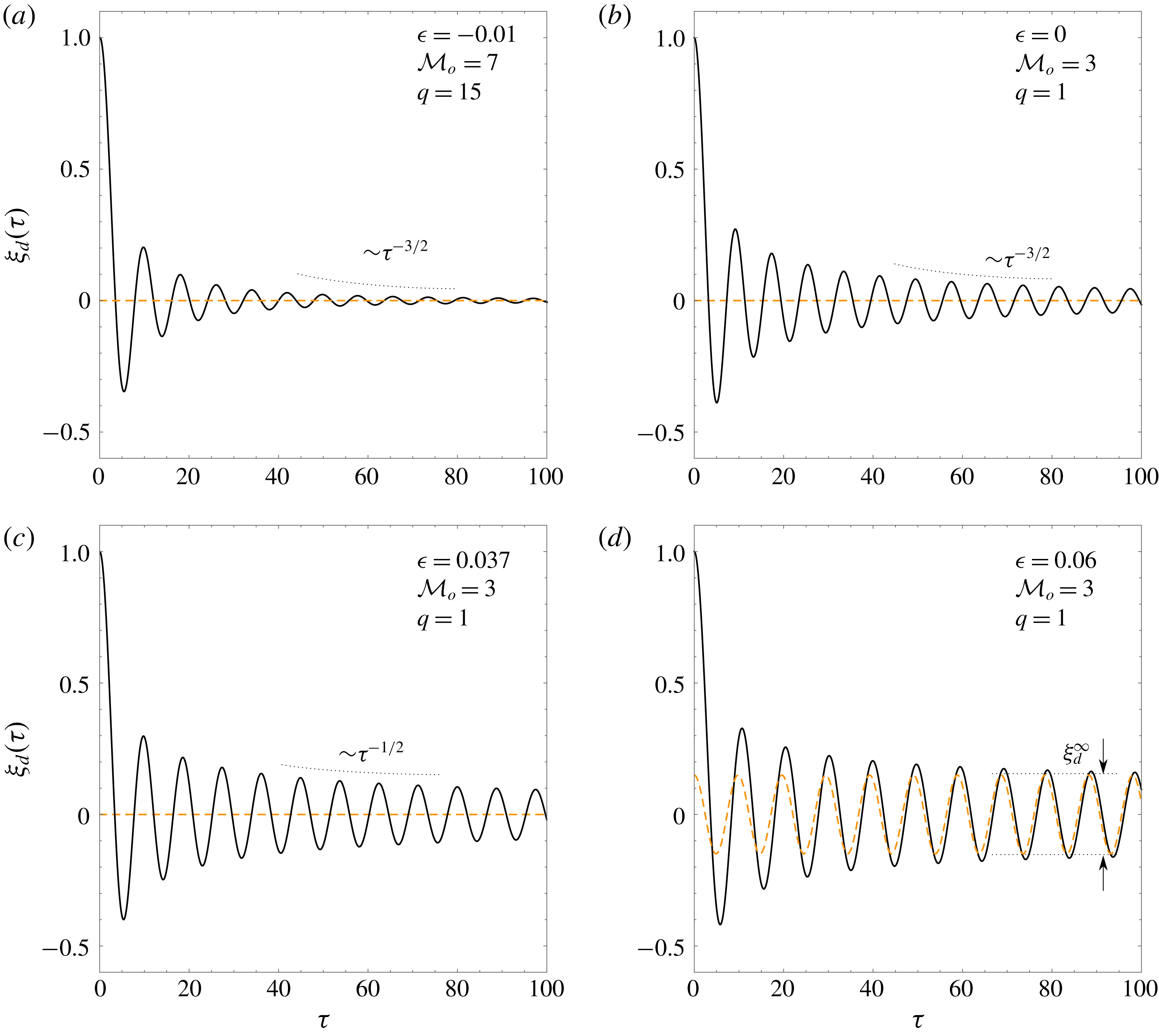
Computations for corrugation amplitude $\unicode[STIX]{x1D709}_{d}(\unicode[STIX]{x1D70F})$ are displayed in figure 7 for ${\mathcal{M}}_{o}=7$ , $q=15$ , $\unicode[STIX]{x1D6FE}=1.3$ and a negative correlation parameter $\unicode[STIX]{x1D716}=-0.01$ (figure 7 a), and for ${\mathcal{M}}_{o}=3$ , $q=1$ , $\unicode[STIX]{x1D6FE}=1.3$ and positive correlation parameters $\unicode[STIX]{x1D716}=0.06$ (figure 7 b), $\unicode[STIX]{x1D716}=0.037$ (figure 7 c) and $\unicode[STIX]{x1D716}=0$ (figure 7 d). It is found that the highly damped oscillating regime, $\unicode[STIX]{x1D70E}_{b}>\unicode[STIX]{x1D70E}_{c}+1/(4\unicode[STIX]{x1D70E}_{c})$ , is obtained in figure 7(a). The case of regular detonations, which is found to lie within the domain $\unicode[STIX]{x1D70E}_{c}>\unicode[STIX]{x1D70E}_{b}<\unicode[STIX]{x1D70E}_{c}+1/(4\unicode[STIX]{x1D70E}_{c})$ , is displayed in figure 7(b). In these two regimes, the amplitude of the detonation ripple oscillations decays with time with the power law $\unicode[STIX]{x1D70F}^{-3/2}$ . The strong attenuation of the detonation-front vibrations in figure 7(a) is associated with the negative correlation with the shock intensity. The higher the shock perturbation towards the fresh mixture, the stronger is the mechanical energy subtracted from the bulk and the weaker is the overall heat release.

Figure 7.

Temporal evolution of the detonation-front ripple amplitude $\unicode[STIX]{x1D709}_{d}(\unicode[STIX]{x1D70F})$ computed for ${\mathcal{M}}_{o}=7$ , $q=15$ , $\unicode[STIX]{x1D6FE}=1.3$ ( $\unicode[STIX]{x1D716}=-0.01$ ), and for ${\mathcal{M}}_{o}=3$ , $q=1$ , $\unicode[STIX]{x1D6FE}=1.3$ ( $\unicode[STIX]{x1D716}=0$ , $0.037$ , $0.06$ ).

Note that the asymptotic decay rate of an isolated Bessel function is $\text{J}_{\unicode[STIX]{x1D708}}(\unicode[STIX]{x1D70F}\gg 1)\sim \unicode[STIX]{x1D70F}^{-1/2}$ , not the power law $\unicode[STIX]{x1D70F}^{-3/2}$ that the complete series in (4.2) displays for adiabatic shocks. For $\unicode[STIX]{x1D70E}_{c}>\unicode[STIX]{x1D70E}_{b}$ , a condition that applies for the two first cases (figures 7 a and 7 b), the leading terms cancel and the remaining leading order dominates the asymptotic expansion (Fraley Reference Fraley1986). When the condition $\unicode[STIX]{x1D70E}_{b}=\unicode[STIX]{x1D70E}_{c}$ is satisfied, a case computed in figure 7(c), the leading terms do not vanish, which renders a decay rate with the power law $\unicode[STIX]{x1D70F}^{-1/2}$ for $\unicode[STIX]{x1D70F}\gg 1$ . For $\unicode[STIX]{x1D70E}_{b}<\unicode[STIX]{x1D70E}_{c}$ , there exists a constant-amplitude contribution added to the time-decaying function. This is readily observed in figure 7(d), where the oscillations at the front reach a non-decaying regime for sufficiently long times, i.e. the DK regime.

A clear distinction of the family of solutions distinguished in figure 4 is also provided in Bates (Reference Bates2004), where the inverse Laplace transform technique renders different late-time asymptotic functions for $\unicode[STIX]{x1D709}_{d}(\unicode[STIX]{x1D70F})$ depending on the equations of state. The highly damped oscillating regime is found to present an exponential contribution that decays faster, and a power-law contribution of the form $\unicode[STIX]{x1D70F}^{-3/2}$ that dominates the long-time state. In particular, we refer to equations (57)–(60) in Bates (Reference Bates2004), which were contrasted against FAST2D hydrodynamical simulations and that have been employed here to check the results given by (4.2). To the best of the authors’ knowledge, similar computations of the type considered here have not been performed.

The expressions that describe the long-time evolution of the detonation front in the DK regime can be obtained by direct inspection of the residues in (A 10) and (A 11), which yields

(4.3) $$\begin{eqnarray}\unicode[STIX]{x1D709}_{d}(\unicode[STIX]{x1D70F}\gg 1)=\unicode[STIX]{x1D709}_{d}^{\infty }\cos (\unicode[STIX]{x1D714}\unicode[STIX]{x1D70F})\end{eqnarray}$$

and

(4.4) $$\begin{eqnarray}\hat{p}_{d}(\unicode[STIX]{x1D70F}\gg 1)=\hat{p}_{d}^{\infty }\sin (\unicode[STIX]{x1D714}\unicode[STIX]{x1D70F})=-\unicode[STIX]{x1D709}_{d}^{\infty }{\displaystyle \frac{\unicode[STIX]{x1D714}}{\unicode[STIX]{x1D70E}_{a}}}\sin (\unicode[STIX]{x1D714}\unicode[STIX]{x1D70F})\end{eqnarray}$$

for the detonation ripple and pressure perturbations, respectively, with the asymptotic amplitude of the detonation shape deviations with respect to the planar shape being

(4.5) $$\begin{eqnarray}\unicode[STIX]{x1D709}_{d}^{\infty }={\displaystyle \frac{\unicode[STIX]{x1D701}_{+}^{2}(\unicode[STIX]{x1D70E}_{b}^{2}-1)+1-\unicode[STIX]{x1D70E}_{b}\unicode[STIX]{x1D70E}_{c}-\unicode[STIX]{x1D70E}_{c}\sqrt{\unicode[STIX]{x1D701}_{+}^{2}-1}}{(\unicode[STIX]{x1D701}_{+}^{2}+\unicode[STIX]{x1D701}_{-}^{2})}}.\end{eqnarray}$$

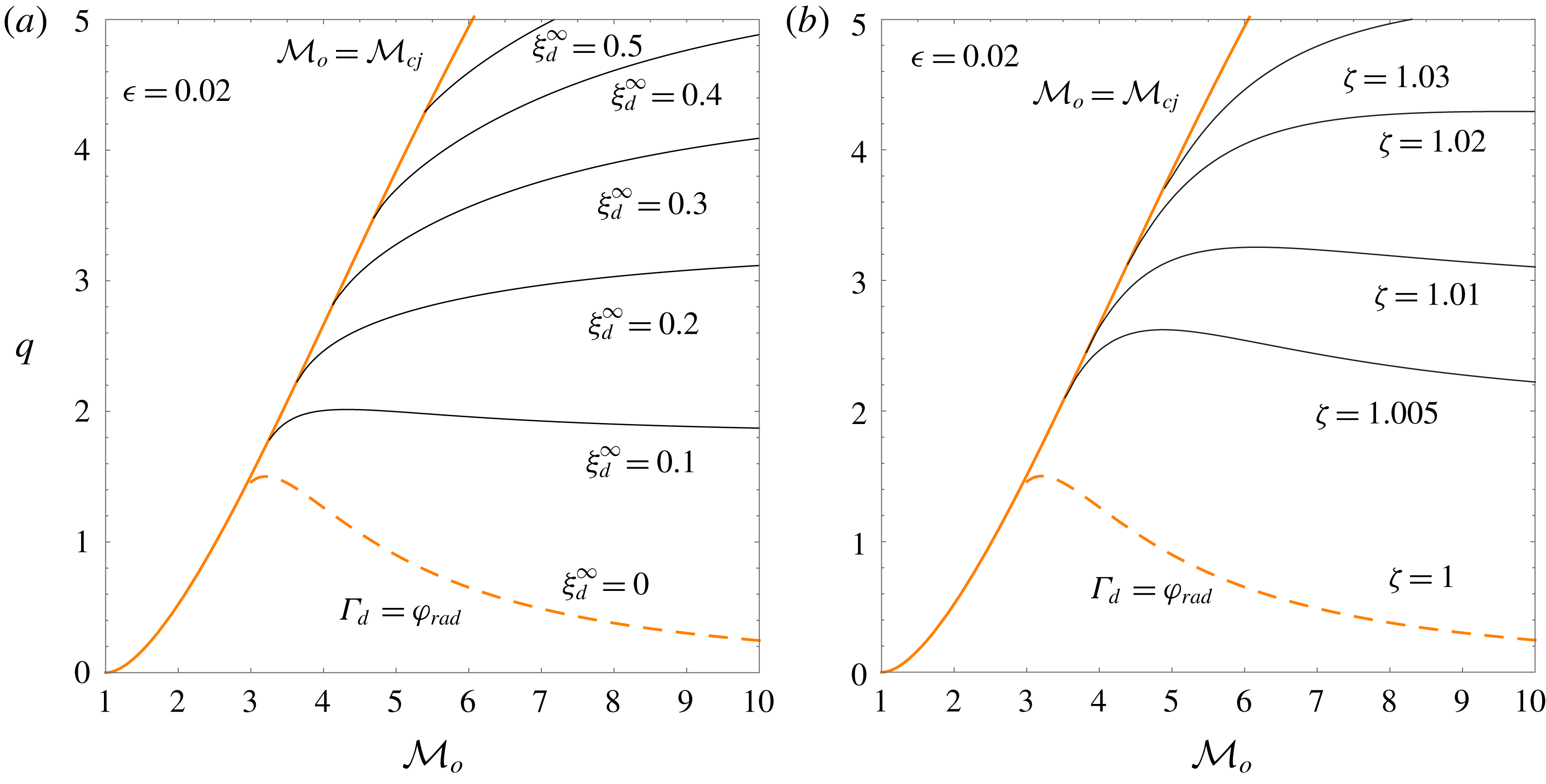
The natural oscillation frequency in the temporal variable $\unicode[STIX]{x1D70F}$ is $\unicode[STIX]{x1D714}=\unicode[STIX]{x1D701}_{-}\sqrt{1-{\mathcal{M}}_{d}^{2}}$ , where the value of $\unicode[STIX]{x1D701}_{-}$ is provided in (3.4). The asymptotic long-time oscillation amplitude $\unicode[STIX]{x1D709}_{d}^{\infty }$ and frequency $\unicode[STIX]{x1D701}_{-}$ are computed in figures 8(a) and 8(b), respectively, for $\unicode[STIX]{x1D6FE}=1.3$ and $\unicode[STIX]{x1D716}=0.02$ . It is seen that $\unicode[STIX]{x1D70E}_{b}=\unicode[STIX]{x1D70E}_{c}$ yields $\unicode[STIX]{x1D701}_{-}=1$ or $\unicode[STIX]{x1D714}=\sqrt{1-{\mathcal{M}}_{d}^{2}}$ corresponding to sound waves running parallel to the detonation surface. It is also observed that, although the amplitude grows with the heat release, the oscillation frequency barely changes since $\unicode[STIX]{x1D701}_{-}$ is found to be roughly unity within the domain $\unicode[STIX]{x1D70E}_{b}<\unicode[STIX]{x1D70E}_{c}$ explored in figure 8. Employing other values of the same order for $\unicode[STIX]{x1D716}$ does not produce any qualitative change in the results.

Figure 8.

Asymptotic detonation ripple amplitude (a) and oscillation frequency (b) as a function of ${\mathcal{M}}_{o}$ and $q$ . The curves have been computed with $\unicode[STIX]{x1D6FE}=1.3$ and $\unicode[STIX]{x1D716}=0.02$ .

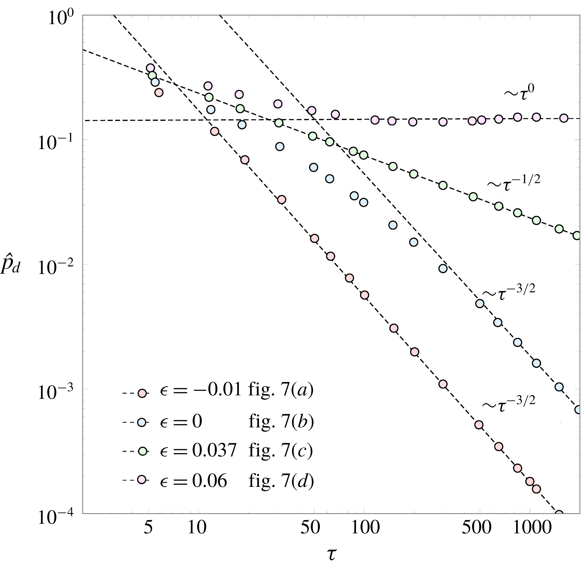
A simple form to inspect the power law that describes the long-time asymptotic decay is to display the peak values of the pressure function in a log–log scale for a sufficiently long temporal domain, and then to compute the corresponding regression lines. This analysis is performed in figure 9 with the same input parameters as those employed in figure 7. The results confirm the previous discussion on the asymptotic long-time limit. It is, however, instructive to check that some configurations, such as that found for $\unicode[STIX]{x1D716}=0$ , demand very long times to fit on the asymptotic trend. In some conditions, the shock must cover distances of the order of 100 perturbation wavelengths. This fact limits the reproducibility of the asymptotic analysis in real configurations, where base-flow changes may occur in the formation and propagation of the reactive front. Besides, the long-time dynamics computed here is based on the isolated-front assumption. It is known, however, that piston coupling effects can effectively modify the stability limits obtained in figure 5, as shown in Freeman (Reference Freeman1955) and Bates (Reference Bates2012, Reference Bates2015). Although the isolated assumption is certainly non-physical for a non-reactive steady shock, detonations can propagate with a high degree of self-sustainability, or can even be totally self-sustained in the CJ regime. The closer to this regime the front is, the weaker are the influences from the downstream boundary conditions, as the coupling is determined by the acoustic field that becomes sonic in CJ conditions.

Figure 9.

Long-time pressure perturbation peaks computed for ${\mathcal{M}}_{o}=3$ , $q=1$ , $\unicode[STIX]{x1D6FE}=1.3$ ( $\unicode[STIX]{x1D716}=0.06$ , $0.037$ , $0$ ), and for ${\mathcal{M}}_{o}=7$ , $q=15$ , $\unicode[STIX]{x1D6FE}=1.3$ ( $\unicode[STIX]{x1D716}=-0.01$ ).

Note that the scaling chosen to define the dimensionless spatial and temporal variables is not appropriate to reproduce CJ conditions, where the downstream flow is strictly sonic, ${\mathcal{M}}_{d}=1$ . Since the oscillation frequency factor in (4.4) is $\sin (\unicode[STIX]{x1D701}_{-}r)=\sin (\unicode[STIX]{x1D714}\unicode[STIX]{x1D70F})$ in the CJ regime, the value $\unicode[STIX]{x1D714}$ approaches zero as $\unicode[STIX]{x1D714}\sim 1-{\mathcal{M}}_{d}^{-2}$ . In other words, pressure perturbations cannot travel in the streamwise direction in sonic conditions, so the acoustic coupling of the pressure field at different positions along the moving detonation front is impossible. It is therefore convenient to derive an asymptotic theory for weakly overdriven detonations such as that provided in § 3.2.

4.2 Burnt-gas flow variables

The pressure field in the burnt-gas flow can be derived with the aid of (A 13) and undoing the hyperbolic variable change carried out in (A 1), namely $\unicode[STIX]{x1D712}=\tanh ^{-1}(x/\unicode[STIX]{x1D70F})$ and $r=\sqrt{\unicode[STIX]{x1D70F}^{2}-x^{2}}$ , to give

(4.6) $$\begin{eqnarray}\hat{p}(x,y,\unicode[STIX]{x1D70F})=\mathop{\sum }_{\unicode[STIX]{x1D708}=0}^{\infty }N_{\unicode[STIX]{x1D708}}\left[{\displaystyle \frac{(1+{\mathcal{M}}_{d})(\unicode[STIX]{x1D70F}-x)}{(1-{\mathcal{M}}_{d})(\unicode[STIX]{x1D70F}+x)}}\right]^{-\unicode[STIX]{x1D708}/2}\text{J}_{\unicode[STIX]{x1D708}}\left(\sqrt{\unicode[STIX]{x1D70F}^{2}-x^{2}}\right)\cos (y).\end{eqnarray}$$

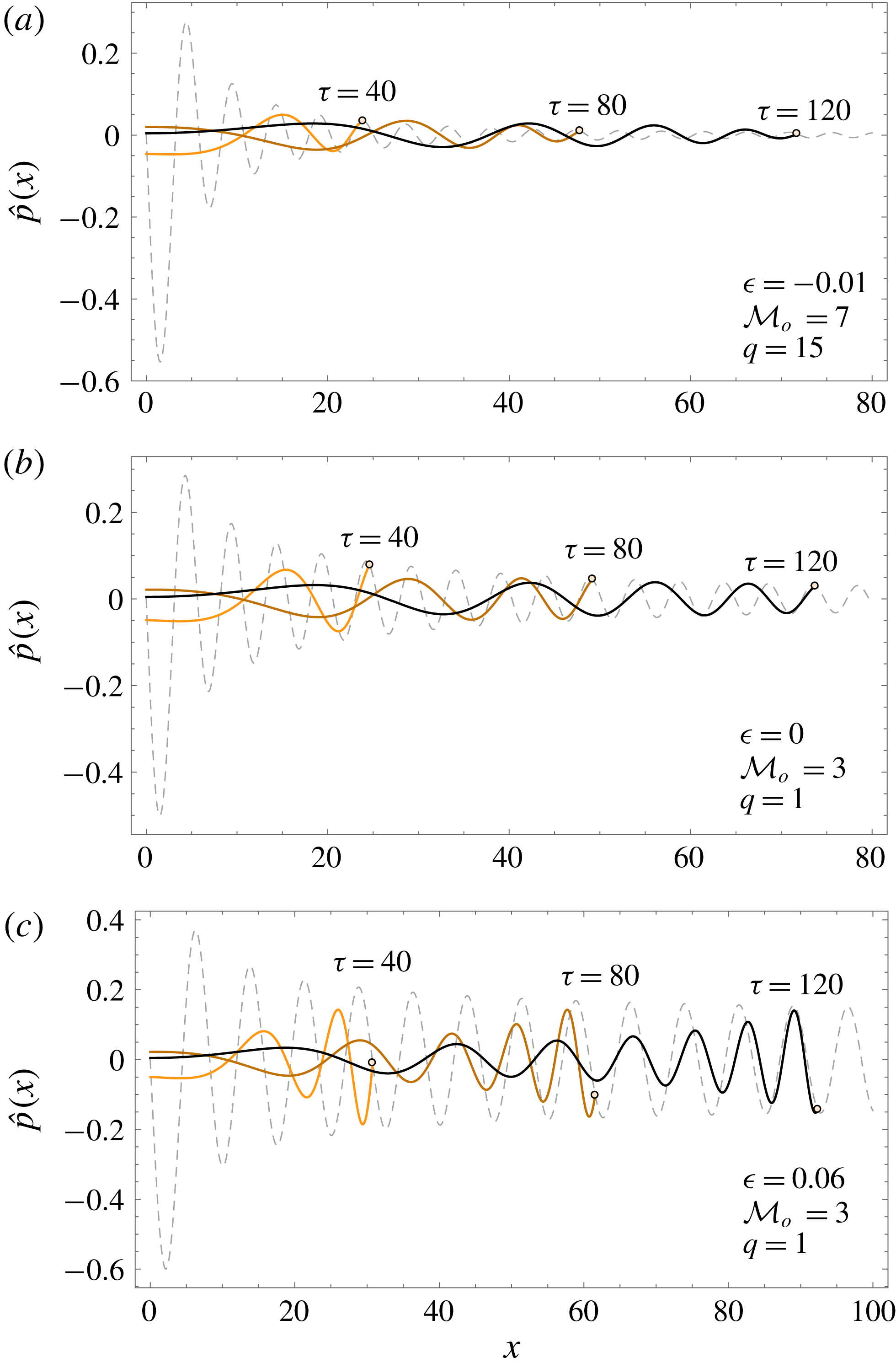
The spatial distribution of the pressure field is computed in figure 10 for the same conditions as in figure 7 for $\unicode[STIX]{x1D70F}=40$ (orange), $\unicode[STIX]{x1D70F}=80$ (brown) and $\unicode[STIX]{x1D70F}=120$  (black). Two regimes are well distinguished: acoustically radiating and non-radiating conditions. The SAE condition is determined by the condition $\unicode[STIX]{x1D701}_{-}>1$ , or equivalently $\unicode[STIX]{x1D714}>(1-{\mathcal{M}}_{d})^{1/2}$ , a condition that is always satisfied in the stable oscillatory mode $\unicode[STIX]{x1D70E}_{b}<\unicode[STIX]{x1D70E}_{c}$ . As previously mentioned, the case $k_{a}<0$ represents acoustic waves travelling in the direction of the post-shock flow, while the waves moving in the opposite direction correspond to $k_{a}>0$ . The solution corresponding to shock oscillation frequency $\unicode[STIX]{x1D714}=1$ is associated with standing acoustic waves that separate the solution travelling to the left, $\unicode[STIX]{x1D714}>1$ , from the one travelling to the right, $(1-{\mathcal{M}}_{d}^{2})^{1/2}<\unicode[STIX]{x1D714}<1$ , in the reference frame comoving with the burnt-gas fluid.

Figure 10.

Spatial vorticity field $\hat{p}$ for $\unicode[STIX]{x1D70F}=40$ (orange), $\unicode[STIX]{x1D70F}=80$ (brown) and $\unicode[STIX]{x1D70F}=120$ (black) for ${\mathcal{M}}_{o}=7$ , $q=15$ , $\unicode[STIX]{x1D716}=-0.01$  (a), for ${\mathcal{M}}_{o}=3$ , $q=1$ , $\unicode[STIX]{x1D716}=0$  (b), and for ${\mathcal{M}}_{o}=3$ , $q=1$ , $\unicode[STIX]{x1D716}=0.06$  (c). The grey dashed line shows the pressure-detonation history.

Sufficiently far from the shock in the burnt gas, i.e. at a distance much longer than the perturbation wavelength, the asymptotic pressure perturbations when the reactive shock oscillates with constant amplitude are given by

(4.7) $$\begin{eqnarray}\hat{p}(x,y,\unicode[STIX]{x1D70F}\gg 1)=\hat{p}_{d}^{\infty }\sin (\unicode[STIX]{x1D701}_{a}\unicode[STIX]{x1D70F}-k_{a}x)\cos (y),\end{eqnarray}$$

where $\hat{p}_{d}^{\infty }$ is the amplitude of the pressure perturbations at the detonation front. Besides the initial-value problem resolved in this work, normal-mode analysis can also be conducted to obtain the asymptotic flow-field variables in the burnt gas.

Associated with the SAE, there exists a sound energy radiation flux that reads  $\boldsymbol{j}=\unicode[STIX]{x1D70C}_{d}^{\prime }a_{d}^{\prime 2}|\hat{p}|^{2}\boldsymbol{v}_{a}^{\prime }$ in the burnt-gas reference frame. The acoustic wavenumber vector that points in the sound compression direction, $\boldsymbol{v}_{a}^{\prime }=a_{d}^{\prime }\boldsymbol{k}_{a}$ , is

(4.8) $$\begin{eqnarray}\boldsymbol{k}_{a}=(\cos \unicode[STIX]{x1D703}_{a},\sin \unicode[STIX]{x1D703}_{a})=\left(\frac{\unicode[STIX]{x1D714}{\mathcal{M}}_{d}-\sqrt{\unicode[STIX]{x1D714}^{2}-1+{\mathcal{M}}_{d}^{2}}}{\unicode[STIX]{x1D714}-{\mathcal{M}}_{d}\sqrt{\unicode[STIX]{x1D714}^{2}-1+{\mathcal{M}}_{d}^{2}}},\frac{1-{\mathcal{M}}_{d}^{2}}{\unicode[STIX]{x1D714}-{\mathcal{M}}_{d}\sqrt{\unicode[STIX]{x1D714}^{2}-1+{\mathcal{M}}_{d}^{2}}}\right),\end{eqnarray}$$

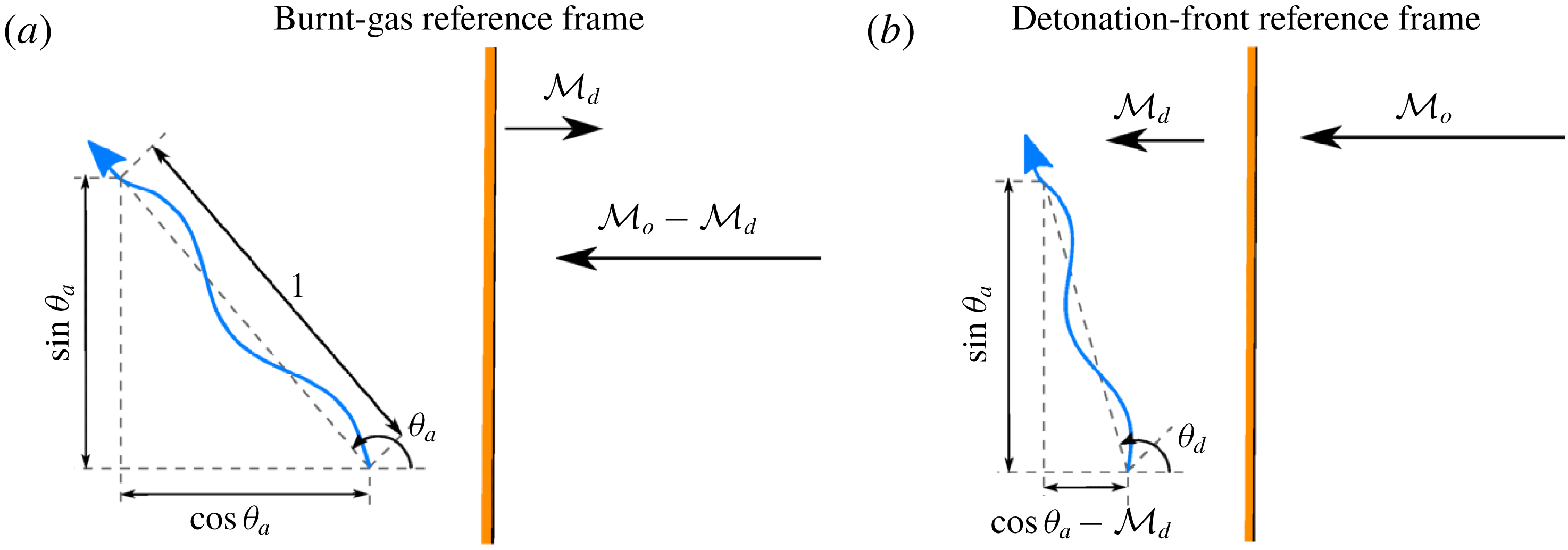
with the characteristic angle $\unicode[STIX]{x1D703}_{a}$ being sketched in figure 11(a).

Computations of the acoustic energy flux can be employed to characterize the noise associated with the unsteadiness of the detonation, as done for regular shocks (Ribner Reference Ribner1969). In applications where the detonation wave remains anchored to the domain boundaries, as they are for supersonic combustors that employ detonations as a way of burning, the analysis is conveniently done in the detonation wave reference frame (see figure 11 b). For that case, the sound energy flux is given by $\boldsymbol{v}_{ad}^{\prime }=a_{d}^{\prime }\boldsymbol{k}_{a}-u_{d}^{\prime }\hat{\boldsymbol{e}}_{x}$ .

Focused on the result of the most interest, the longitudinal projection is calculated scaled with the zero-order energy flux $\unicode[STIX]{x1D70C}_{d}^{\prime }a_{d}^{\prime 3}$ , thereby yielding

(4.9) $$\begin{eqnarray}J_{d}=(1-{\mathcal{M}}_{d}\cos \unicode[STIX]{x1D703}_{a})({\mathcal{M}}_{d}-\cos \unicode[STIX]{x1D703}_{a})|\hat{p}_{d}|^{2},\end{eqnarray}$$

as the dimensionless acoustic radiation, where the corresponding emission angle

(4.10) $$\begin{eqnarray}\cos \unicode[STIX]{x1D703}_{d}={\displaystyle \frac{\cos \unicode[STIX]{x1D703}_{a}-{\mathcal{M}}_{d}}{\sqrt{1+{\mathcal{M}}_{d}^{2}-2{\mathcal{M}}_{d}\cos \unicode[STIX]{x1D703}_{a}}}}\end{eqnarray}$$

is determined by the vectors $\hat{\boldsymbol{e}}_{x}$ and $\boldsymbol{v}_{ad}^{\prime }/|\boldsymbol{v}_{ad}^{\prime }|$ . The acoustic energy flux adds second-order corrections to the density, velocity and pressure behind the detonation wave, as well as mass, momentum and energy fluxes. Such deviations affect the overall velocity propagation, since the RH relations get modified by these second-order corrections (Velikovich, Huete & Wouchuk Reference Velikovich, Huete and Wouchuk2012).

Figure 11.

Sketch of the sound-wave emission angle when measured in the burnt-gas reference frame (a) and detonation-front reference frame (b).

It is immediate to see that $\unicode[STIX]{x1D701}_{-}\gtrsim 1$ implies $\cos \unicode[STIX]{x1D703}_{a}\sim {\mathcal{M}}_{d}$ and $\unicode[STIX]{x1D703}_{d}\sim \unicode[STIX]{x03C0}/2$ . In view of the computations displayed in figure 8, this is a representative condition within the oscillatory mode, $\unicode[STIX]{x1D70E}_{b}<\unicode[STIX]{x1D70E}_{c}$ . Therefore, for scenarios where the rippled detonation oscillates with a non-decaying amplitude, i.e. when the overdrive is sufficiently low and $\unicode[STIX]{x1D716}>0$ , the pressure field is dominated by transverse waves moving parallel to the detonation surface. Longitudinal acoustic radiation $\unicode[STIX]{x1D703}_{a}\sim \unicode[STIX]{x1D703}_{d}\sim \unicode[STIX]{x03C0}$ would occur when the detonation front experiences high-frequency oscillations $\unicode[STIX]{x1D701}_{-}\gg 1$ , such as those occurring in forced-oscillating conditions imposed by external excitation (Huete et al. Reference Huete, Sánchez and Williams2013, Reference Huete, Jin, Martínez and Luo2017).

The isentropic density and temperature variations induced by the acoustic radiation are simply given by $\hat{\unicode[STIX]{x1D70C}}_{a}(x,y,\unicode[STIX]{x1D70F})=\hat{p}(x,y,\unicode[STIX]{x1D70F})$ and $\hat{T}_{a}(x,y,\unicode[STIX]{x1D70F})=(\unicode[STIX]{x1D6FE}-1)\hat{p}(x,y,\unicode[STIX]{x1D70F})$ , respectively, with the pressure function $\hat{p}$ being previously given in (4.6) and displayed in figure 10.

The breakdown of the velocity field into acoustic and rotational contributions, namely $\hat{u} (x,y,t)=\hat{u} _{a}(x,y,t)+\hat{u} _{r}(x,y)$ and $\hat{v}(x,y,t)=\hat{v}_{a}(x,y,t)+\hat{v}_{r}(x,y)$ for the streamwise and lateral components, respectively, facilitates the problem resolution. As readily seen from the Euler equations, the acoustic contribution of the velocity fluctuations obeys

(4.11a,b ) $$\begin{eqnarray}\frac{\unicode[STIX]{x2202}^{2}\hat{u} _{a}}{\unicode[STIX]{x2202}\unicode[STIX]{x1D70F}^{2}}=\frac{\unicode[STIX]{x2202}^{2}\hat{u} _{a}}{\unicode[STIX]{x2202}x^{2}}\quad \text{and}\quad \frac{\unicode[STIX]{x2202}^{2}\hat{v}_{a}}{\unicode[STIX]{x2202}\unicode[STIX]{x1D70F}^{2}}=-\hat{v}_{a},\end{eqnarray}$$

for the longitudinal and transverse components, respectively. It is, however, simpler to withdraw the acoustic velocity perturbations from the momentum conservation equations in (2.12d ). On the other hand, the steady-rotational perturbations, which are isobaric in the linear limit, are governed by

(4.12a,b ) $$\begin{eqnarray}\frac{\unicode[STIX]{x2202}^{2}\hat{u} _{r}}{\unicode[STIX]{x2202}x^{2}}-\hat{u} _{r}=\unicode[STIX]{x1D6FA}\quad \text{and}\quad \frac{\unicode[STIX]{x2202}^{2}\hat{v}_{r}}{\unicode[STIX]{x2202}x^{2}}-\hat{v}_{r}=-\frac{\unicode[STIX]{x2202}\unicode[STIX]{x1D6FA}}{\unicode[STIX]{x2202}x},\end{eqnarray}$$

where the function

(4.13) $$\begin{eqnarray}\unicode[STIX]{x1D6FA}(x,y)=\frac{\unicode[STIX]{x2202}\hat{v}}{\unicode[STIX]{x2202}x}-\frac{\unicode[STIX]{x2202}\hat{u} }{\unicode[STIX]{x2202}y}=\frac{(1-\unicode[STIX]{x1D6E4}_{d})({\mathcal{R}}_{d}^{2}-1)}{2{\mathcal{M}}_{d}}\hat{p}_{d}\left(\unicode[STIX]{x1D70F}=\frac{\sqrt{1-{\mathcal{M}}_{d}^{2}}}{{\mathcal{M}}_{d}}x\right)\sin (y)\end{eqnarray}$$

represents the dimensionless vorticity field. In the absence of diffusive effects, the vorticity–entropy perturbations in the burnt gas can only be generated at the detonation front.

In many applications, the upstream gas is not uniform and contains density and velocity disturbances (Huete et al. Reference Huete, Sánchez and Williams2013, Reference Huete, Jin, Martínez and Luo2017). For such cases, the vorticity deposited in the burnt gas is affected by other contributions, as the amplification of the vorticity ahead of the front might be as a direct result of the overall compression ratio and the baroclinic generation. The latter occurs when there are density and/or pressure gradients in the direction transverse to the detonation propagation direction.

Similar to the velocity perturbations, the total density field comprises acoustic and entropic contributions, $\hat{\unicode[STIX]{x1D70C}}(x,y,t)=\hat{\unicode[STIX]{x1D70C}}_{a}(x,y,t)+\hat{\unicode[STIX]{x1D70C}}_{e}(x,y)$ . The latter can be readily obtained from the linearized RH equation (2.15c ) after subtracting the acoustic part, yielding

(4.14) $$\begin{eqnarray}\hat{\unicode[STIX]{x1D70C}}_{e}(x,y)=\frac{\unicode[STIX]{x1D6E4}_{d}-{\mathcal{M}}_{d}^{2}}{{\mathcal{M}}_{d}^{2}}\hat{p}_{d}\left(\unicode[STIX]{x1D70F}=\frac{\sqrt{1-{\mathcal{M}}_{d}^{2}}}{{\mathcal{M}}_{d}}x\right)\cos (y).\end{eqnarray}$$

The vorticity and entropy perturbations generated in the far field can be determined by the asymptotic detonation evolution. While the planar detonation does not generate any vorticity–entropy perturbation in the long-time regime for $\unicode[STIX]{x1D70E}_{b}>\unicode[STIX]{x1D70E}_{c}$ , there exist vortical and entropic disturbances in the burnt gas for $\unicode[STIX]{x1D70E}_{b}<\unicode[STIX]{x1D70E}_{c}$ , which take the following form:

(4.15) $$\begin{eqnarray}\unicode[STIX]{x1D6FA}(x\gg 1,y)=\frac{(1-\unicode[STIX]{x1D6E4}_{d})({\mathcal{R}}_{d}^{2}-1)}{2{\mathcal{M}}_{d}}\hat{p}_{d}^{\infty }\sin \left(\unicode[STIX]{x1D70F}=\frac{\sqrt{1-{\mathcal{M}}_{d}^{2}}}{{\mathcal{M}}_{d}}x\right)\sin (y)\end{eqnarray}$$

and

(4.16) $$\begin{eqnarray}\hat{\unicode[STIX]{x1D70C}}_{e}(x\gg 1,y)=\frac{\unicode[STIX]{x1D6E4}_{d}-{\mathcal{M}}_{d}^{2}}{{\mathcal{M}}_{d}^{2}}\hat{p}_{d}^{\infty }\sin \left(\unicode[STIX]{x1D70F}=\frac{\sqrt{1-{\mathcal{M}}_{d}^{2}}}{{\mathcal{M}}_{d}}x\right)\cos (y),\end{eqnarray}$$

respectively.

Figure 12.

Isocontours of the vorticity field $\unicode[STIX]{x1D6FA}$ for ${\mathcal{M}}_{o}=7$ , $q=15$ , $\unicode[STIX]{x1D716}=-0.01$  (a), for ${\mathcal{M}}_{o}=3$ , $q=1$ , $\unicode[STIX]{x1D716}=0$  (b), and for ${\mathcal{M}}_{o}=3$ , $q=1$ , $\unicode[STIX]{x1D716}=0.06$  (c).

The spatial distribution of the vorticity left in the burnt-gas particles is computed in figure 12 for ${\mathcal{M}}_{o}=7$ , $q=15$ , $\unicode[STIX]{x1D716}=-0.01$ (a), and for ${\mathcal{M}}_{o}=3$ , $q=1$ , $0$ (b) and $\unicode[STIX]{x1D716}=0.06$ (c). Figure 12(a,b) displays a vorticity field that decays with the distance $x$ , as the detonation pressure decays with time as shown in figure 10. Figure 12(c), corresponding to DK conditions, $\unicode[STIX]{x1D70E}_{b}<\unicode[STIX]{x1D70E}_{c}$ , shows a vorticity field that renders order-of-unity values of $\unicode[STIX]{x1D6FA}(x\gg 1)$ , in consonance with figure 10. The maximum and minimum values are located at $y=\pm \unicode[STIX]{x03C0}/2$  ( $\sin y=\pm 1$ ) for $-\unicode[STIX]{x03C0}<y<\unicode[STIX]{x03C0}$ , as they correspond to positions where the tangential velocity is the highest. The qualitative picture of the steady-density field is similar to that represented in figure 12 for the vorticity field, but shifted $\unicode[STIX]{x03C0}/2$ in the transverse direction (see the dependence on the transverse coordinate) and with the iso-curve scaling being modified according to the factors accompanying the function $\hat{p}_{d}$ in (4.13) and (4.14).