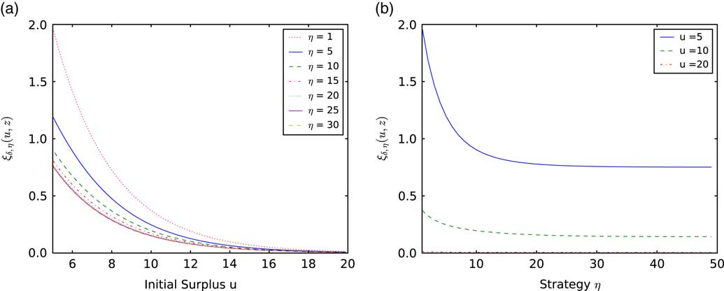
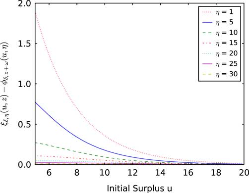
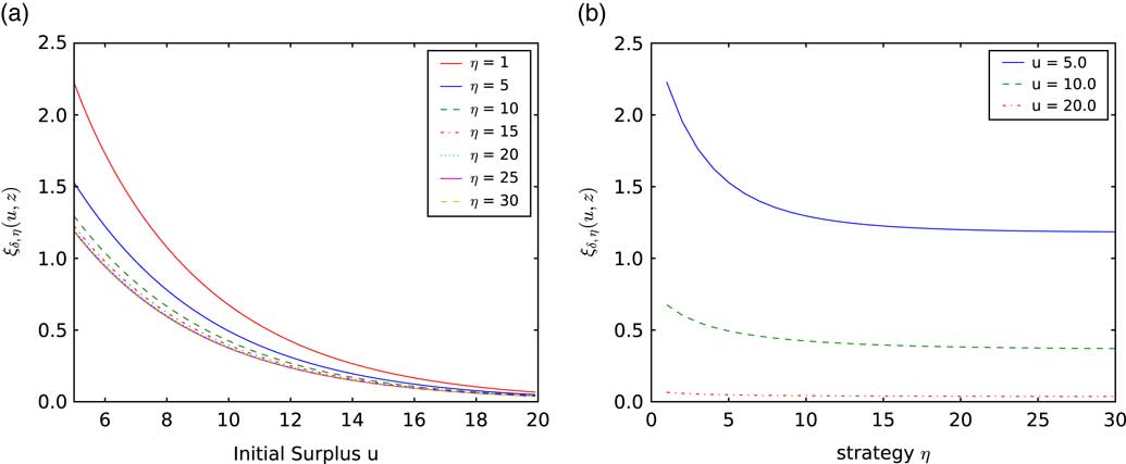
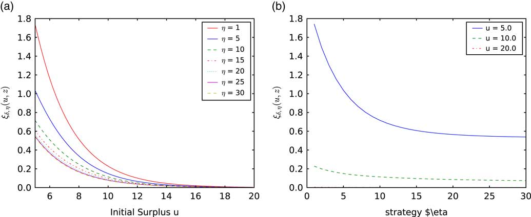
1 Introduction and background

Many researchers have discussed various risk models with different capital injection strategies. The problem of capital injection usually arises from two directions: one is related to insolvency reinsurance contract, where the capital injections keep the insurer alive forever (e.g. Pafumi, Reference Pafumi1998) or away from insolvency (e.g. Nie et al., Reference Nie, Dickson and Li2011; Nie et al., Reference Nie, Dickson and Li2015). In particular, Nie et al. (Reference Nie, Dickson and Li2011) assumed that capital injections only protect against insolvency (which is defined as the surplus falling below a certain level between its initial surplus and zero), and ruin (i.e. dropping below zero) is still possible. In this case, under the assumption of a fixed amount of funds, the optimal retention level in the reinsurance contract which minimises ruin probability was studied. Another direction is related to a by-product of optimal dividend problems, for which the capital injections are regarded as the reinvestment of the shareholders. In the dividend strategy problem considered by de Finetti, the optimal strategy usually leads the insurer's surplus process to ruin with probability one. To avoid such an event, Dickson & Waters (Reference Dickson and Waters2004) introduced a particular type of capital injections which are made by shareholders whenever the surplus drops below zero. We also refer interested readers to Kulenko & Schmidli (Reference Kulenko and Schmidli2008), Eisenberg & Schmidli (Reference Eisenberg and Schmidli2011a, Reference Eisenberg and Schmidli2011b), Avanzi et al. (Reference Avanzi, Shen and Wong2011), Yao et al. (Reference Yao, Yang and Wang2011), Zhou & Yuen (Reference Zhou and Yuen2012) and Zhao et al. (Reference Zhao, Wang, Yao and Chen2015) for the study of different optimal dividend and reinsurance problems in the presence of capital injections in similar risk models. We point out that capital injection is usually a background setting for the study of optimal dividend or reinsurance problems in the papers mentioned above. In other words, capital injection is not the main quantity of interest, but instead the injections are made passively to prevent a ruin event or to reduce the ruin probability. In this paper, we are interested in some alternative capital injection plans set by insurance managers to assist risk management for insurance companies. Instead of the usual capital injection strategy (injecting capital whenever the surplus drops below a certain level), we propose that capital injection plan is scheduled at a predetermined time which is set based on the embedded claim counting process. To be specific, the surplus level is checked at which the accumulated number of claims since the last checkpoint reaches a predetermined value, and if it is below a minimum requirement level then the capital equivalent to the shortfall amount from a minimum requirement level is injected. A reasonable choice of this predetermined number of claims used for capital injection decision lies between the expected number of claims causing surplus being below the minimum requirement and zero. For the study related to the expected number of claims, we refer to Dos Reis (Reference Dos Reis2002), Dickson (Reference Dickson2012) and Li & Lu (Reference Li and Lu2016), etc. Noting that under this proposed capital injection plan, ruin can occur between scheduled capital injection checks. In light of this, it has some similarities but also should be differentiated to those capital injection strategies under randomised observations (e.g. see Zhang et al., Reference Zhang, Cheung and Yang2018). In the literature, Albrecher et al. (Reference Albrecher, Cheung and Thonhauser2011, Reference Albrecher, Cheung and Thonhauser2013) introduced randomised observations for the study of dividend problem and the Gerber–Shiu function, in which Erlang distributed observation intervals can be used to approximate deterministic periodic observations. See also Asmussen et al. (Reference Asmussen, Avram and Usabel2002), Ramaswami et al. (Reference Ramaswami, Woolford and Stanford2008), Stanford et al. (Reference Stanford, Avram, Badescu, Breuer, Soares and Latouche2005, Reference Stanford, Yu and Ren2011) for early use of this Erlangisation technique to study finite-time ruin probabilities. While the so-called Erlangian-inter-observation is suitable for situations such as accounting/reporting purpose, dividend policy and reinsurance agreement which are scheduled independently from the surplus process, in this paper, we focus on a plan that schedules the capital injection time points by utilising some information related to the risk process (i.e. the cumulated number of claims).

We also remark that this kind of capital injection model bears some similarities to the preventive maintenance (PM) policy of shock and damage models in reliability theory. For example, if an operating unit needs to be repaired or replaced whenever it fails, this can be a time-consuming and costly process. Then some necessary maintenance of the unit can be done before its failure to avoid any unexpected breakdown, and this action is called the PM policy. Among various conditions which determine the necessity of maintenance, the cumulated number of shocks is one of the important factors chosen in the context of shock and damage models. If the unit experiences some shocks before the total damage exceeds a predetermined figure, then the PM action is taken. For a thorough discussion and the study of this PM policy in a shock and damage model, see Nakagawa (Reference Nakagawa2006, Reference Nakagawa2007), for example. Also, when a system fails, the corrective maintenance (CM), which is a repair action, is performed in this situation. This is the case corresponding to the ruin situation. As it will be clear later, the expected total discounted capital injection (defined in (2.3)) is defined by taking both PM and CM actions into account.

The rest of the paper is organised as follows. In the subsequent section, we propose and describe in detail a risk model with a PM-type capital injection plan. The primary quantity of our interest is the expected total discounted capital injection until the first ruin time. In section 3, we first introduce a defective discounted density of the surplus level at claim instants, which is a key quantity for later analysis. Its explicit form is given under the assumption of a combination of exponentials claim sizes. Subsequently, section 4 focusses on finding an expression of the expected total discounted capital injection. In turn, a similar expression for the Laplace transform of the time to ruin under the present capital injection risk model is given in section 5. Some numerical examples are provided in section 6 to illustrate how the choices of the predetermined number of claims influences the values of the expected total discounted capital injection and the Laplace transform of time to ruin. In addition, optimal capital injection strategies are numerically studied under the criteria of minimising expected discounted capital injection per unit time until ruin. The paper is concluded with some remarks and discussion for the future research in section 7.

2 The proposed model

In this article, we assume that the insurer’s surplus process prior to any capital injections (which is denoted as {R(t)} _t≥0) follows the classical Poisson risk model. The aggregate claim process is defined as $S\left( t \right){\equals}\mathop{\sum}\nolimits_{i{\equals}1}^{M_{t} } {X_{i} } $ with S(t)=0 if M _t =0, where {M _t } _t≥0 is a Poisson process with intensity λ>0 and $\{ X_{i} \} _{{i{\equals}1}}^{\infty} $ is an independent and identical distributed (iid) sequence of continuous positive random variables (rvs) for the claim sizes with common cumulative distribution function F, and Laplace–Stieltjes transform $$\tilde{f}\left( s \right){\equals}{\int}_0^\infty {e^{{{\minus}sx}} dF\left( x \right)} $$ . Let $$\left\{ {W_{i} } \right\}_{{i\geq 1}}^{\infty} $$ be an iid sequence of continuous positive rvs following exponential distribution with mean 1/λ for the interarrival times. With generic rvs of X _i and W _i for i=1, 2, … , denoted as X and W, respectively, it is assumed that X and W are independent. The premium is collected continuously with rate c=(1+θ)λμ, where μ= $${\Bbb E}$$ (X) and θ>0 is the security loading. With an initial capital u≥0, the insurer’s surplus level at time t is given as

(2.1) $$R\left( t \right){\equals}u{\plus}ct{\minus}S\left( t \right),\quad \quad t\geq 0$$

Here a major variation imposed to the classical Poisson risk model is that there is a predetermined minimum solvency level z>0. We expect that insurers want to analyse how to get a balance between solvency and profitability such that the surplus can stay above the level z longer by paying an acceptable amount of expenses (including injected capital and any associated costs) at some scheduled times. Here we propose a discrete-type capital injection plan scheduled based on the cumulated number of claims. When the cumulated number of claims reaches a predetermined number η, we check the surplus level. At each time of checkpoint, if the surplus level falls below the solvency level z, then capital injection is made to restore the surplus level to z. We also assume that when ruin occurs, the surplus is recovered to z with an immediate individual capital injection which includes z plus a penalty amount linked to the deficit at ruin. Then the process restarts at z. Thus it is sufficient to study a behaviour of the risk process until the first ruin time. Now the modified risk process under the capital injection plan η is defined as

(2.2) $$R^{\eta } \left( t \right){\equals}u{\plus}ct{\minus}S\left( t \right){\plus}U_{t}^{\eta } ,\,t\,\gt\,0$$

where $U_{t}^{\eta } $ is the total capital amounts injected until time t. Let τ ^η =inf{t>0:R ^η (t)<0} be the time of ruin in this modified process (2.2), whereas τ=inf{t>0:R(t)<0} be the time of ruin in the baseline classical risk process (2.1).

In this paper, we study the expected total discounted capital injection until the first ruin time defined as

(2.3) $$\xi _{{\delta ,i}} \left( {u,z} \right){\equals}{\Bbb E}\left[ {\mathop{{\int}_{[0,\tau ^{\eta }]}} {e^{{{\minus}\delta t}} dU_{t}^{\eta } {\Bbb 1}\left\{ {\tau ^{\eta } \,\lt\,\infty} \right\}\!\!\mid\!\!\\R^{\eta } \left( 0 \right){\equals}u,I_{0} {\equals}i{\rm }} } \right],\quad i{\equals}1,2,\,\ldots\,,\eta ,\quad u\geq 0$$

where δ>0 is a discount rate, $${\Bbb 1}$$ {} is an indicator function, and I _t an index function at time t representing the number of claims remaining until the next capital injection check time. Later, in section 4, it will be shown that (2.3) is expressed in terms of (2.3) when i=η for u≥z, and thus we focus on studying ξ _δ,η (u, z) analytically and numerically. Note that the integration in (2.3) is essentially written as a summation

$$\mathop{{\int}_{[0,\tau ^{\eta } ]}} {e^{{{\minus}\delta t}} dU_{t}^{\eta } {\equals}\mathop{\sum}\limits_{i{\equals}1}^\infty {e^{{{\minus}\delta T_{i}^{\eta } }} \left[ {z{\minus}R^{\eta } \left( {T_{i}^{\eta } } \right)} \right]_{{\plus}} {\Bbb 1}\left\{ {T_{i}^{\eta } \,\lt\,\tau ^{\eta } } \right\}{\plus}e^{{{\minus}\delta \tau ^{\eta } }} \left[ {z{\plus}\omega \left( {\mid\!\!\\R^{\eta } \left( {\tau ^{\eta } } \right)\!\!\mid} \right)} \right]} } $$

where (a−b)₊=max(a−b, 0) and $T_{i}^{\eta } $ for i=1, 2 … , are times of checking the surplus level and implementing capital injection if necessary before the first ruin time. In the sequel, in order to obtain an explicit and simple expression for (2.3), we assume that the claim size distribution follows a combination of exponentials with a probability density function (pdf)

(2.4) $$f\left( x \right){\equals}\mathop{\sum}\limits_{i{\equals}1}^\kappa {p_{i} \beta _{i} e^{{{\minus}\beta _{i} x}} ,\quad \quad x\,\gt\,0} $$

where β _i >0 are distinct for all i=1, 2, … , κ and p _i are real quantities such that $\mathop{\sum}\nolimits_{i{\equals}1}^\kappa {p_{i} {\equals}1} $ . Without loss of generality, we assume that β ₁<β ₂< … <β _κ . Since a combination of exponentials is dense in the set of distributions on ℝ⁺ (e.g. Dufresne, Reference Dufresne2007), this assumption is appropriate to a certain extent.

Lastly, for notational convenience, let

(2.5) $$r{\equals}{{\lambda {\plus}\delta } \over c}\quad {\rm and}\quad C_{i} {\equals}{\lambda \over c}\left( {{{p_{i} \beta _{i} } \over {\beta _{i} {\plus}r}}} \right)$$

3 The Discounted Density of the Surplus Level at Claim Instants

To begin, since the surplus level at those potential capital injection time points is a key element in our analysis, we first introduce the defective discounted density of the surplus level at each claim instant. This quantity has its own interest in the literature, we refer to, for example, Stanford & Stroiński (Reference Stanford and Stroinski1994), Stanford et al. (Reference Stanford, Stroinski and Lee2000) and Lu (Reference Lu2016).

Let us denote the density of the generic increment rv Z=cW−X to be g(y) and its discounted density to be g _δ (y). In the classical Poisson risk model, let us consider a bivariate Laplace transform for interclaim time W and increment rv Z=cW−X, namely

(3.1) $${\Bbb E}\big[ {e^{{{\minus}\delta W{\minus}sZ}} } \big]{\equals}{\Bbb E}\big[ {e^{{{\minus}\delta W{\minus}s(cW{\minus}X)}} } \big]{\equals}{\int}_0^\infty {e^{{{\minus}\delta t}} \lambda e^{{{\minus}\lambda t}} } {\int}_0^\infty {{\rm \ztbnd }e^{{{\minus}s\left( {ct{\minus}x} \right)}} f\left( x \right)dx\,dt} .$$

As (3.1) is equivalent to the Laplace transform of g _δ (y), that is, $${\int}_{{\minus}\infty}^\infty {e^{{{\minus}sy}} g_{\delta } \left( y \right)dy} $$ , with a change of variables and an interchange of the order of integration, inversion of Laplace transform yields

(3.2) $$g_{\delta } \left( y \right){\equals}\left\{ {\matrix{ {{\lambda \over c}e^{{{\minus}{{\lambda {\plus}\delta } \over c}y}} \tilde{f}\left( {{{\lambda {\plus}\delta } \over c}} \right),} \hfill &#x0026; {y\,\gt\,0} \hfill \cr {{\int}_0^\infty {{\lambda \over c}e^{{{\minus}{{\lambda {\plus}\delta } \over c}t}} f\left( {t{\minus}y} \right)dt} ,} \hfill &#x0026; {y\leq 0} \hfill \cr } } \right.$$

When δ=0, the density of the generic increment rv Z is

(3.3) $$g(y){\equals}\left\{ {\matrix{ {{\lambda \over c}e^{{{\minus}{\lambda \over c}y}} \tilde{f}\left( {{\lambda \over c}} \right),} \hfill &#x0026; {y\,\gt\,0} \hfill \cr {{\int}_0^\infty {{\lambda \over c}e^{{{\minus}{\lambda \over c}t}} f\left( {t{\minus}y} \right)dt} ,} \hfill &#x0026; {y\leq 0} \hfill \cr } } \right.$$

See Stanford & Stroiński (Reference Stanford and Stroinski1994) and Stanford et al. (Reference Stanford, Stroinski and Lee2000) for the form of the distribution of increment Z in more general claim arrival processes.

But, from (2.4), one has $\tilde{f}\left( {{\lambda \over c}} \right){\equals}\mathop{\sum}\nolimits_{i{\equals}1}^\kappa {{{p_{i} \beta _{i} } \over {\beta _{i} {\plus}{\lambda \over c}}}} $ and thus

$${\int}_0^\infty {{\lambda \over c}e^{{{\minus}{{\lambda {\plus}\delta } \over c}t}} f\left( {t{\minus}y} \right)dt{\equals}{\lambda \over c}\mathop{\sum}\limits_{i{\equals}1}^\kappa {p_{i} \beta _{i} {\int}_0^\infty {{\rm \ztbnd }e^{{{\minus}{{\lambda {\plus}\delta } \over c}t}} e^{{{\minus}\beta _{i} \left( {t{\minus}y} \right)}} dt{\equals}{\lambda \over c}} } \mathop{\sum}\limits_{i{\equals}1}^\kappa {{{p_{i} \beta _{i} } \over {\beta _{i} {\plus}{{\lambda {\plus}\delta } \over c}}}e^{{\beta _{i} y}} } } .$$

Consequently one finds (3.2) in this case

(3.4) $$g_{\delta } \left( y \right){\equals}\left\{ {\matrix{ {\mathop{\sum}\nolimits_{i{\equals}1}^\kappa {C_{i} e^{{{\minus}ry}} } ,} \hfill &#x0026; {y\,\gt\,0} \hfill \cr {\mathop{\sum}\nolimits_{i{\equals}1}^\kappa {C_{i} e^{{\beta _{i} y}} } ,} \hfill &#x0026; {y\leq 0} \hfill \cr } } \right.$$

where r and C _i are given by (2.5).

Next, let

(3.5) $$h_{n} \left( {u,x} \right)dx{\equals}{\rm Pr}\left( {R\left( {T_{n} } \right)\in{dx,\tau \,\gt\,T_{n} \!\mid\\\!R\left( 0 \right){\equals}u} \right),\quad \quad u\geq 0$$

be the defective density of the surplus level immediately after the nth claim given that ruin has not yet occurred, where $T_{n} {\equals}\mathop{\sum}\nolimits_{i{\equals}1}^n {W_{i} } $ is the arrival time of nth claim. Using (3.4), its discounted defective density of the surplus level after the first claim is given as

(3.6) $$h_{{\delta ,1}} \left( {u,x} \right){\equals}\left\{ {\matrix{ {\mathop{\sum}\nolimits_{i{\equals}1}^\kappa {C_{i} e^{{{\minus}r\left( {x{\minus}u} \right)}} ,} } \hfill &#x0026; {x\,\gt\,u} \hfill \cr {\mathop{\sum}\nolimits_{i{\equals}1}^\kappa {C_{i} e^{{\beta _{i} \left( {x{\minus}u} \right)}} ,} } \hfill &#x0026; {0\leq x\leq u} \hfill \cr } } \right.$$

For n≥2, by Markov property

(3.7) $$h_{{\delta ,n}} \left( {u,x} \right){\equals}{\int}_0^\infty {h_{{\delta ,n{\minus}1}} \left( {u,y} \right)h_{{\delta ,1}} \left( {y,x} \right)dy} $$

Also, it is convenient to introduce some technical results involving the tail of Erlang distribution $${\int}_x^\infty {{{\beta ^{k} y^{{k{\minus}1}} } \over {\left( {k{\minus}1} \right)\,!\,}}e^{{{\minus}\beta y}} dy} {\equals}\mathop{\sum}\nolimits_{h{\equals}0}^{k{\minus}1} {{{\left( {\beta x} \right)^{h} e^{{{\minus}\beta x}} } \over {h\,!\,}}} ,$$ which are

(3.8) $$\left\{ {\matrix{ {{\int}_x^\infty {{{y^{{k{\minus}1}} } \over {\left( {k{\minus}1} \right)\,!\,}}e^{{{\minus}\beta y}} dy} {\equals}\mathop{\sum}\nolimits_{h{\equals}1}^k {{{x^{{h{\minus}1}} e^{{{\minus}\beta x}} } \over {\beta ^{{k{\plus}1{\minus}h}} \left( {h{\minus}1} \right)\,!\,}}} } \cr {{\int}_0^x {{{y^{{k{\minus}1}} } \over {\left( {k{\minus}1} \right)\,!\,}}e^{{{\minus}\beta y}} dy{\equals}{1 \over {\beta ^{k} }}} {\minus}\mathop{\sum}\nolimits_{h{\equals}1}^k {{{x^{{h{\minus}1}} e^{{{\minus}\beta x}} } \over {\beta ^{{k{\plus}1{\minus}h}} \left( {h{\minus}1} \right)\,!\,}}} } \cr } } \right.$$

Note that the form of the second equation is still valid when β<0, but the first equation is only well-defined for β>0.

(3.9) $$h_{{\delta ,n}} \left( {u,x} \right){\equals}\mathop{\sum}\limits_{i{\equals}1}^\kappa {\mathop{\sum}\limits_{j{\equals}1}^{n{\minus}1} {\mathop{\sum}\limits_{k{\equals}1}^{n{\minus}j} {A_{{n,i,j,k}} {{u^{{j{\minus}1}} x^{{k{\minus}1}} } \over {\left( {j{\minus}1} \right)\,!\,\left( {k{\minus}1} \right)\,!\,}}e^{{{\minus}\beta _{i} u{\minus}rx}} {\plus}} } } \mathop{\sum}\limits_{j{\equals}1}^n {B_{{n,j}}^{{\left( 1 \right)}} {{\left( {x{\minus}u} \right)^{{j{\minus}1}} } \over {\left( {j{\minus}1} \right)\,!\,}}} e^{{{\minus}r\left( {x{\minus}u} \right)}} $$

and when 0≤x≤u

(3.10) $$h_{{\delta ,n}} \left( {u,x} \right){\equals}\mathop{\sum}\limits_{i{\equals}1}^\kappa {\mathop{\sum}\limits_{j{\equals}1}^{n{\minus}1} {\mathop{\sum}\limits_{k{\equals}1}^{n{\minus}j} {A_{{n,i,j,k}} {{u^{{j{\minus}1}} x^{{k{\minus}1}} } \over {\left( {j{\minus}1} \right)\,!\,\left( {k{\minus}1} \right)\,!\,}}e^{{{\minus}\beta _{i} u{\minus}rx}} {\plus}} } } \mathop{\sum}\limits_{i{\equals}1}^\kappa {\mathop{\sum}\limits_{j{\equals}1}^n {B_{{n,i,j}}^{{\left( 2 \right)}} {{\left( {u{\minus}x} \right)^{{j{\minus}1}} } \over {\left( {j{\minus}1} \right)\,!\,}}e^{{\beta _{i} \left( {x{\minus}u} \right)}} } } $$

where the coefficients A _n,i,j,k , $B_{{n,j}}^{{\left( 1 \right)}} $ and $B_{{n,i,j}}^{{\left( 2 \right)}} $ are determined recursively as

(3.11) $$\left\{ {\matrix{ &#x0026;{A_{{n{\plus}1,i,j,k}} {\equals}\mathop{\sum}\nolimits_{h{\equals}k}^{n{\minus}j} {\mathop{\sum}\nolimits_{l{\equals}1}^\kappa {{{A_{{n,i,j,h}} B_{{1,l,1}}^{{(2)}} } \over {\left( {\beta _{l} {\plus}r} \right)^{{h{\plus}1{\minus}k}} }}{\plus}A_{{n,i,j,k{\minus}1}} B_{{1,1}}^{{\left( 1 \right)}} {\Bbb 1}\left\{ {k\,\ne\,1} \right\}} } {\minus}\mathop{\sum}\nolimits_{l{\equals}j}^n {{{B_{{n,i,l}}^{{\left( 2 \right)}} B_{{1,1}}^{{\left( 1 \right)}} } \over {\left( {\beta _{i} {\plus}r} \right)^{{l{\plus}1{\minus}j}} }}{\Bbb 1}\left\{ {k{\equals}1} \right\}} ,} \cr &#x0026;{{\rm for}\quad i{\equals}1,2\,\ldots\,,\kappa ,\,j{\equals}1,2,\,\ldots\,n{\minus}1,\,k{\equals}1,2,\,\ldots\,,n{\plus}1{\minus}j,} \cr &#x0026;\hskip-10pc{A_{{n{\plus}1,i,n,1}} {\equals}{\minus}{{B_{{n,i,n}}^{{\left( 2 \right)}} B_{{1,1}}^{{\left( 1 \right)}} } \over {\beta _{i} {\plus}r}},\,{\rm for}\quad i{\equals}1,2,\,\ldots\,,\kappa ,\,j{\equals}n,\,k{\equals}1,} \cr } } \right.$$

(3.12) $$\left\{ {\matrix{ {B_{{n{\plus}1,j}}^{{\left( 1 \right)}} {\equals}\mathop{\sum}\nolimits_{l{\equals}j}^n {\mathop{\sum}\nolimits_{i{\equals}1}^\kappa {{{B_{{n,l}}^{{\left( 1 \right)}} B_{{1,i,1}}^{{\left( 2 \right)}} } \over {\left( {\beta _{i} {\plus}r} \right)^{{l{\plus}1{\minus}j}} }}{\plus}B_{{n,j{\minus}1}}^{{\left( 1 \right)}} B_{{1,1}}^{{\left( 1 \right)}} {\Bbb 1}\left\{ {j\,\ne\,1} \right\}} } {\plus}\mathop{\sum}\nolimits_{k{\equals}1}^n {\mathop{\sum}\nolimits_{i{\equals}1}^\kappa {{{B_{{n,i,k}}^{{\left( 2 \right)}} B_{{1,1}}^{{\left( 1 \right)}} } \over {\left( {\beta _{i} {\plus}r} \right)^{k} }}{\Bbb 1}\left\{ {j{\equals}1} \right\}} } } \cr {{\rm for}\quad j{\equals}1,2,\,\ldots\,,n} \cr &#x0026;\hskip-45pc{B_{{n{\plus}1,n{\plus}1}}^{{\left( 1 \right)}} {\equals}B_{{n,n}}^{{\left( 1 \right)}} B_{{1,1}}^{{\left( 1 \right)}} ,\,{\rm for}\quad j{\equals}n{\plus}1} \cr } } \right.$$

and

(3.13) $$\left\{ {\matrix{ {B_{{n{\plus}1,i,j}}^{{(2)}} {\equals}\mathop{\sum}\nolimits_{l{\equals}j}^n {{{B_{{n,i,l}}^{{(2)}} B_{{1,1}}^{{(1)}} } \over {\left( {\beta _{i} {\plus}r} \right)^{{l{\plus}1{\minus}j}} }}} {\plus}\mathop{\sum}\nolimits_{k{\equals}1}^n {{{B_{{1,i,1}}^{{(2)}} B_{{n,k}}^{{(1)}} } \over {\left( {\beta _{i} {\plus}r} \right)^{k} }}{\Bbb 1}\{ j{\equals}1\} } {\minus}\mathop{\sum}\nolimits_{l{\equals}j}^n {\mathop{\sum}\nolimits_{k{\equals}1\atop \hskip-1pt k\, \ne\,i}^\kappa {{{B_{{n,i,l}}^{{(2)}} B_{{1,k,1}}^{{(2)}} } \over {\left( {\beta _{i} {\minus}\beta _{k} } \right)^{{l{\plus}1{\minus}j}} }}} } } \cr {{\plus}B_{{n,i,j{\minus}1}}^{{(2)}} B_{{1,i,1}}^{{(2)}} {\Bbb 1}\left\{ {j\,\ne\,1} \right\}{\plus}\mathop{\sum}\nolimits_{l{\equals}1}^n {\mathop{\sum}\nolimits_{k{\equals}1\atop \hskip-1pt k\,\ne\,i}^\kappa {{{B_{{n,k,l}}^{{(2)}} B_{{1,i,1}}^{{(2)}} } \over {\left( {\beta _{k} {\minus}\beta _{i} } \right)^{l} }}{\Bbb 1}\left\{ {j{\equals}1} \right\}} } } \cr {{\rm for}\quad i{\equals}1,2,\,\ldots\,,\,\kappa ,\,j{\equals}1,2,\,\ldots\,,n} \cr &#x0026;\hskip-32pc{B_{{n{\plus}1,i,n{\plus}1}}^{{(2)}} {\equals}B_{{n,i,n}}^{{(2)}} B_{{1,i,1}}^{{(2)}} ,\,{\rm for}\quad i{\equals}1,2,\,\ldots\,,\kappa ,\,j{\equals}n{\plus}1} \cr } } \right.$$

with the initial values

(3.14) $$B_{{1,1}}^{{(1)}} {\equals}\mathop \sum\limits_{i{\equals}1}^\kappa C_{i} $$

(3.15) $$B_{{1,i,1}}^{{(2)}} {\equals}C_{i} ,\quad \quad i{\equals}1,2,\,\ldots\,,\kappa $$

(3.16) $$A_{{2,i,1,1}} {\equals}{\minus}{{B_{{1,1}}^{{(1)}} B_{{1,i,1}}^{{(2)}} } \over {\beta _{i} {\plus}r}}{\equals}{\minus}\mathop{\sum}\limits_{l{\equals}1}^\kappa {{{C_{l} C_{i} } \over {\beta _{i} {\plus}r}}\quad \quad } i{\equals}1,2,...,\kappa $$

(3.17) $$h_{{\delta ,2}} \left( {u,x} \right){\equals}{\int}_0^\infty {h_{{\delta ,1}} \left( {u,y} \right)h_{{\delta ,1}} \left( {y,x} \right)dy} {\equals}\mathop{{\int}_D} {h_{{\delta ,1}} \left( {u,y} \right)h_{{\delta ,1}} \left( {y,x} \right)dy} $$

where $D{\equals}{\cup} _{{i{\equals}1}}^{4} D_{i} $ with $$D_{1} {\equals}\left\{ {y\,\colon\,\left\{ {y\,\gt\,u} \right\}{\cap} \left\{ {x\,\gt\,y} \right\}} \right\}$$ , $D_{2} {\equals}\left\{ {y\,\colon\,\left\{ {y\,\gt\,u} \right\}{\cap} \left\{ {x\leq y} \right\}} \right\},\,D_{3} {\equals}$ $\left\{ {y\,\colon\,\left\{ {y\leq u} \right\}{\cap} \left\{ {x\,\gt\,y} \right\}} \right\}$ , and $D_{4} {\equals}\left\{ {y\,\colon\,\left\{ {y\leq u} \right\}{\cap} \left\{ {x\leq y} \right\}} \right\}$ . Using (3.6), the terms on the right-hand side of (3.17) are expressed as

(3.18) $$\eqalignno{ \mathop{{\int}_{D_{1} }} {h_{{\delta ,1}} \left( {u,y} \right)h_{{\delta ,1}} \left( {y,x} \right)dy} {\equals}{\int}_u^x {B_{{1,1}}^{{\left( 1 \right)}} B_{{1,1}}^{{\left( 1 \right)}} e^{{{\minus}r\left( {x{\minus}u} \right)}} {\Bbb 1}\left\{ {x\,\gt\,u} \right\}dy} \cr &#x0026;\hskip-130pt{\!\equals}B_{{1,1}}^{{(1)}} B_{{1,1}}^{{(1)}} \left( {x{\minus}u} \right)e^{{{\minus}r\left( {x{\minus}u} \right)}} {\Bbb 1}\left\{ {x\,\gt\,u} \right\} $$

(3.19) $$\eqalignno{ \mathop{{\int}_{D_2}_} {h_{{\delta ,1}} \left( {u,y} \right)h_{{\delta ,1}} \left( {y,x} \right)dy} {\equals}{\int}_{{\rm max}(x,u)}^\infty {B_{{1,1}}^{{(1)}} } \mathop{\sum}\limits_{i{\equals}1}^\kappa {B_{{1,i,1}}^{{(2)}} e^{{{\minus}(\beta _{i} {\plus}r)y}} e^{{ru{\plus}\beta _{i} x}} dy} \cr &#x0026;\hskip-170pt {\equals}\mathop \sum\limits_{i{\equals}1}^\kappa {{B_{{1,i,1}}^{{(2)}} B_{{1,1}}^{{(1)}} } \over {\beta _{i} {\plus}r}}e^{{{\minus}r(x{\minus}u)}} {\Bbb 1}\left\{ {x\,\gt\,u} \right\}{\plus}\mathop \sum\limits_{i{\equals}1}^\kappa {{B_{{1,i,1}}^{{(2)}} B_{{1,1}}^{{(1)}} } \over {\beta _{i} {\plus}r}}e^{{\beta _{i} (x{\minus}u)}} {\Bbb 1}\left\{ {x\leq u} \right\} $$

(3.20) $$\hskip 2pt\eqalignno{\hskip-5.2pc\,\mathop{{\int}_{D_3}} {h_{{\delta ,1}} \left( {u,y} \right)h_{{\delta ,1}} \left( {y,x} \right)dy} {\equals}{\int}_0^{{\rm min}(x,u)} {\mathop{\sum}\limits_{i{\equals}1}^\kappa {B_{{1,i,1}}^{{(2)}} B_{{1,1}}^{{(1)}} e^{{(\beta _{i} {\plus}r)y}} e^{{{\minus}\beta _{i} u{\minus}rx}} dy} {\rm \ztbnd }} \cr &#x0026; \hskip-166pt{\equals}\mathop{\sum}\limits_{i{\equals}1}^\kappa {B_{{1,i,1}}^{{(2)}} B_{{1,1}}^{{(1)}} e^{{{\minus}\beta _{i} u{\minus}rx}} } {\int}_0^{{\rm min}(x,u)} {e^{{(\beta _{i} {\plus}r)y}} dy} \cr &#x0026; \hskip-166pt{\equals}\mathop \sum\limits_{i{\equals}1}^\kappa {{B_{{1,i,1}}^{{(2)}} B_{{1,1}}^{{(1)}} } \over {\beta _{i} {\plus}r}}e^{{{\minus}r(x{\minus}u)}} {\Bbb 1}\left\{ {x\,\gt\,u} \right\}\cr &#x0026; \hskip-158pt{\plus}\mathop \sum\limits_{i{\equals}1}^\kappa {{B_{{1,i,1}}^{{(2)}} B_{{1,1}}^{{(1)}} } \over {\beta _{i} {\plus}r}}e^{{\beta _{i} (x{\minus}u)}} {\Bbb 1}\left\{ {x\leq u} \right\}{\minus}\mathop \sum\limits_{i{\equals}1}^\kappa {{B_{{1,i,1}}^{{(2)}} B_{{1,1}}^{{(1)}} } \over {\beta _{i} {\plus}r}}e^{{{\minus}\beta _{i} u{\minus}rx}} $$

and

(3.21) $$\eqalignno{ \mathop {\int \limits_{D_4}} h_{{\delta ,1}} \left( {u,y} \right)h_{{\delta ,1}} \left( {y,x} \right)dy{\equals}{\int}_x^u {\mathop \sum\limits_{i{\equals}1}^\kappa B_{{1,i,1}}^{{(2)}} \mathop \sum\limits_{j{\equals}1}^\kappa B_{{1,j,1}}^{{(2)}} e^{{(\beta _{i} {\minus}\beta _{j} )y}} e^{{{\minus}\beta _{i} u{\plus}\beta _{j} x}} {\Bbb 1}\left\{ {x\leq u} \right\}dy} \cr &#x0026; \hskip-207pt {\equals}\left[ {\mathop \sum\limits_{i{\equals}1}^\kappa \mathop{\sum}\limits_{\scriptstyle j{\equals}1 \hfill \atop \scriptstyle j\,\ne\,i \hfill} ^\kappa {{{B_{{1,i,1}}^{{(2)}} B_{{1,j,1}}^{{(2)}} } \over {\beta _{i} {\minus}\beta _{j} }}e^{{\beta _{j} (x{\minus}u)}} } {\minus}\mathop \sum\limits_{i{\equals}1}^\kappa \mathop{\sum}\limits_{\scriptstyle j{\equals}1 \hfill \atop \scriptstyle j\,\ne\,i \hfill} ^\kappa {{{B_{{1,i,1}}^{{(2)}} B_{{1,j,1}}^{{(2)}} } \over {\beta _{i} {\minus}\beta _{j} }}e^{{\beta _{i} (x{\minus}u)}} } } \right]{\Bbb 1}\left\{ {x\leq u} \right\} \cr &#x0026; \hskip-200pt{\plus}\mathop \sum\limits_{i{\equals}1}^\kappa {\rm \ztbnd }B_{{1,i,1}}^{{(2)}} B_{{1,i,1}}^{{(2)}} \left( {u{\minus}x} \right)e^{{\beta _{i} (x{\minus}u)}} {\Bbb 1}\left\{ {x\leq u} \right\} $$

Combining (3.18)–(3.21), it follows that (3.9) and (3.10) with the coefficients in (3.11)–(3.16) hold true for n=2.

Next, we assume that (3.9) and (3.10) hold for some n≥3, then (3.7) for n+1 becomes

(3.22) $$\eqalignno{ h_{{\delta ,n{\plus}1}} \left( {u,x} \right){\equals}{\int}_0^\infty {h_{{\delta ,n}} \left( {u,y} \right)h_{{\delta ,1}} \left( {y,x} \right)dy} \cr &#x0026; \hskip-108pt{\equals}{\int}_0^\infty {\mathop \sum\limits_{i{\equals}1}^\kappa \mathop \sum\limits_{j{\equals}1}^{n{\minus}1} \mathop \sum\limits_{k{\equals}1}^{n{\minus}j} {\rm \ztbnd }A_{{n,i,j,k}} {{u^{{j{\minus}1}} y^{{k{\minus}1}} } \over {\left( {j{\minus}1} \right)\,!\,\left( {k{\minus}1} \right)\,!\,}}{\rm }e^{{{\minus}\beta _{i} u{\minus}ry}} h_{{\delta ,1}} \left( {y,x} \right)dy} \cr &#x0026; \hskip-102pt{\plus}{\int}_u^\infty {\mathop \sum\limits_{j{\equals}1}^n B_{{n,j}}^{{(1)}} {{\left( {y{\minus}u} \right)^{{j{\minus}1}} } \over {\left( {j{\minus}1} \right)\,!\,}}\,e^{{{\minus}r(y{\minus}u)}} h_{{\delta ,1}} \left( {y,x} \right)dy} \cr &#x0026; \hskip-102pt{\plus}{\int}_0^u {\mathop \sum\limits_{i{\equals}1}^\kappa \mathop \sum\limits_{j{\equals}1}^n {\rm \ztbnd }B_{{n,i,j}}^{{(2)}} {{\left( {u{\minus}y} \right)^{{j{\minus}1}} } \over {\left( {j{\minus}1} \right)!\,}}{\rm }e^{{\beta _{i} (y{\minus}u)}} h_{{\delta ,1}} \left( {y,x} \right)dy} $$

Upon substitution of (3.6) into (3.22), the three integrals on the right-hand side are re-expressed as follows. The first integral is

$$\eqalignno{ {\int}_0^\infty {\mathop \sum\limits_{i{\equals}1}^\kappa \mathop \sum\limits_{j{\equals}1}^{n{\minus}1} \mathop \sum\limits_{k{\equals}1}^{n{\minus}j} A_{{n,i,j,k}} {{u^{{j{\minus}1}} y^{{k{\minus}1}} } \over {\left( {j{\minus}1} \right)!\,\left( {k{\minus}1} \right)!\,}}{\rm }e^{{{\minus}\beta _{i} u{\minus}ry}} h_{{\delta ,1}} \left( {y,x} \right)dy} \cr &#x0026; \hskip-170pt{\equals}\mathop \sum\limits_{i{\equals}1}^\kappa \mathop \sum\limits_{j{\equals}1}^{n{\minus}1} \mathop{\sum}\limits_{k{\equals}1}^{n{\minus}j} {A_{{n,i,j,k}} {{u^{{j{\minus}1}} } \over {\left( {j{\minus}1} \right)!\,}}B_{{1,1}}^{{(1)}} \left[ {{\int}_0^x {{{y^{{k{\minus}1}} } \over {\left( {k{\minus}1} \right)!\,}}e^{{{\minus}\beta _{i} u{\minus}rx}} dy} } \right]} \cr &#x0026; \hskip-164pt{\rm }{\plus}\mathop \sum\limits_{i{\equals}1}^\kappa \mathop \sum\limits_{j{\equals}1}^{n{\minus}1} \mathop \sum\limits_{k{\equals}1}^{n{\minus}j} A_{{n,i,j,k}} {{u^{{j{\minus}1}} } \over {\left( {j{\minus}1} \right)!\,}}\mathop \sum\limits_{l{\equals}1}^\kappa B_{{1,l,1}}^{{(2)}} \left[ {{\int}_x^\infty {{{y^{{k{\minus}1}} } \over {\left( {k{\minus}1} \right)!\,}}e^{{{\minus}(\beta _{l} {\plus}r)y}} dy} } \right]e^{{{\minus}\beta _{i} u{\plus}\beta _{l} x}} \cr &#x0026; \hskip-170pt{\equals}\mathop \sum\limits_{i{\equals}1}^\kappa \mathop \sum\limits_{j{\equals}1}^{n{\minus}1} \mathop \sum\limits_{k{\equals}1}^{n{\minus}j} A_{{n,i,j,k}} {{u^{{j{\minus}1}} } \over {\left( {j{\minus}1} \right)!\,}}B_{{1,1}}^{{(1)}} {{x^{k} } \over {k!\,}}e^{{{\minus}\beta _{i} u{\minus}rx}} \cr &#x0026; \hskip-164pt{\rm }{\plus}\mathop \sum\limits_{i{\equals}1}^\kappa \mathop \sum\limits_{j{\equals}1}^{n{\minus}1} \mathop \sum\limits_{k{\equals}1}^{n{\minus}j} {\rm \ztbnd }A_{{n,i,j,k}} {{u^{{j{\minus}1}} } \over {\left( {j{\minus}1} \right)!\,}}\mathop \sum\limits_{l{\equals}1}^\kappa B_{{1,l,1}}^{{(2)}} \mathop \sum\limits_{h{\equals}1}^k {{x^{{h{\minus}1}} } \over {\left( {\beta _{l} {\plus}r} \right)^{{k{\plus}1{\minus}h}} \left( {h{\minus}1} \right)!\,}}e^{{{\minus}\beta _{i} u{\minus}rx}} , $$

where the last equality is due to (3.8). A change of variables and interchanging the order of summation yield

(3.23) $$\eqalignno{ {\int}_0^\infty {\mathop \sum\limits_{i{\equals}1}^\kappa \mathop \sum\limits_{j{\equals}1}^{n{\minus}1} \mathop \sum\limits_{k{\equals}1}^{n{\minus}j} A_{{n,i,j,k}} {{u^{{j{\minus}1}} y^{{k{\minus}1}} } \over {\left( {j{\minus}1} \right)!\,\left( {k{\minus}1} \right)!\,}}{\rm }e^{{{\minus}\beta _{i} u{\minus}ry}} h_{{\delta ,1}} \left( {y,x} \right)dy} \cr &#x0026; \hskip-170pt{\equals}\mathop \sum\limits_{i{\equals}1}^\kappa \mathop \sum\limits_{j{\equals}1}^{n{\minus}1} \mathop \sum\limits_{k{\equals}2}^{n{\plus}1{\minus}j} A_{{n,i,j,k{\minus}1}} B_{{1,1}}^{{(1)}} {{u^{{j{\minus}1}} x^{{k{\minus}1}} } \over {\left( {j{\minus}1} \right)!\,\left( {k{\minus}1} \right)!\,}}e^{{{\minus}\beta _{i} u{\minus}rx}} \cr &#x0026; \hskip-164pt{\plus}\mathop \sum\limits_{i{\equals}1}^\kappa \mathop \sum\limits_{j{\equals}1}^{n{\minus}1} \mathop \sum\limits_{k{\equals}1}^{n{\minus}j} \mathop \sum\limits_{h{\equals}k}^{n{\minus}j} \mathop \sum\limits_{l{\equals}1}^\kappa {{A_{{n,i,j,h}} B_{{1,l,1}}^{{(2)}} } \over {\left( {\beta _{l} {\plus}r} \right)^{{h{\plus}1{\minus}k}} }}{{u^{{j{\minus}1}} x^{{k{\minus}1}} } \over {\left( {j{\minus}1} \right)!\,\left( {k{\minus}1} \right)!\,}}e^{{{\minus}\beta _{i} u{\minus}rx}} $$

With the use of (3.8), the second integral is

(3.24) $$\eqalignno{ {\int}_u^\infty {\mathop \sum\limits_{j{\equals}1}^n B_{{n,j}}^{{(1)}} {{\left( {y{\minus}u} \right)^{{j{\minus}1}} } \over {\left( {j{\minus}1} \right)!\,}}e^{{{\minus}r(y{\minus}u)}} h_{{\delta ,1}} \left( {y,x} \right)dy} \cr &#x0026; \hskip-130pt{\equals}\mathop \sum\limits_{j{\equals}1}^n B_{{n,j}}^{{(1)}} B_{{1,1}}^{{(1)}} {\int}_u^x {{{\left( {y{\minus}u} \right)^{{j{\minus}1}} } \over {\left( {j{\minus}1} \right)!\,}}e^{{{\minus}r(x{\minus}u)}} {\Bbb 1}\left\{ {x\,\gt\,u} \right\}dy} \cr &#x0026; \hskip-124pt{\plus}\mathop \sum\limits_{j{\equals}1}^n B_{{n,j}}^{{(1)}} \mathop \sum\limits_{i{\equals}1}^\kappa B_{{1,i,1}}^{{(2)}} e^{{\beta _{i} x{\plus}ru}} {\int}_{{\rm max}(x,u)}^\infty {{{\left( {y{\minus}u} \right)^{{j{\minus}1}} } \over {\left( {j{\minus}1} \right)!\,}}e^{{{\minus}(\beta _{i} {\plus}r)y}} dy} \cr &#x0026; \hskip-130pt{\equals}\mathop \sum\limits_{j{\equals}2}^{n{\plus}1} B_{{n,j{\minus}1}}^{{(1)}} B_{{1,1}}^{{(1)}} {{\left( {x{\minus}u} \right)^{{j{\minus}1}} } \over {\left( {j{\minus}1} \right)!\,}}e^{{{\minus}r(x{\minus}u)}} {\Bbb 1}\left\{ {x\,\gt\,u} \right\} \cr &#x0026; \hskip-124pt{\plus}\mathop \sum\limits_{j{\equals}1}^n \mathop \sum\limits_{i{\equals}1}^\kappa B_{{n,j}}^{{(1)}} B_{{1,i,1}}^{{(2)}} \mathop \sum\limits_{l{\equals}1}^j {{(x{\minus}u)^{{l{\minus}1}} } \over {\left( {\beta _{i} {\plus}r} \right)^{{j{\plus}1{\minus}l}} \left( {l{\minus}1} \right)!\,}}e^{{{\minus}r(x{\minus}u)}} {\Bbb 1}\left\{ {x\,\gt\,u} \right\} \cr &#x0026; \hskip-124pt{\plus}\mathop \sum\limits_{j{\equals}1}^n \mathop \sum\limits_{i{\equals}1}^\kappa B_{{n,j}}^{{(1)}} B_{{1,i,1}}^{{(2)}} {1 \over {\left( {\beta _{i} {\plus}r} \right)^{j} }}e^{{\beta _{i} (x{\minus}u)}} {\Bbb 1}\left\{ {x\leq u} \right\} $$

The last integral in (3.22) is

(3.25) $$\eqalignno{ {\int}_0^u {\mathop \sum\limits_{i{\equals}1}^\kappa \mathop \sum\limits_{j{\equals}1}^n B_{{n,i,j}}^{{(2)}} {{\left( {u{\minus}y} \right)^{{j{\minus}1}} } \over {\left( {j{\minus}1} \right)!\,}}e^{{\beta _{i} (y{\minus}u)}} h_{{\delta ,1}} \left( {y,x} \right)dy} \cr &#x0026; \hskip-135pt{\equals}\mathop \sum\limits_{i{\equals}1}^\kappa \mathop \sum\limits_{j{\equals}1}^n B_{{n,i,j}}^{{(2)}} B_{{1,1}}^{{(1)}} e^{{{\minus}\beta _{i} u{\minus}rx}} {\int}_0^{{\rm min}(x,u)} {{{\left( {u{\minus}y} \right)^{{j{\minus}1}} } \over {\left( {j{\minus}1} \right)!\,}}e^{{(\beta _{i} {\plus}r)y}} dy} \cr &#x0026; \hskip-130pt{\plus}\mathop \sum\limits_{i{\equals}1}^\kappa \mathop \sum\limits_{j{\equals}1}^n B_{{n,i,j}}^{{(2)}} \mathop \sum\limits_{l{\equals}1}^\kappa B_{{1,l,1}}^{{(2)}} e^{{{\minus}\beta _{i} u{\plus}\beta _{l} x}} {\int}_x^u {{{\left( {u{\minus}y} \right)^{{j{\minus}1}} } \over {\left( {j{\minus}1} \right)!\,}}{\rm }e^{{(\beta _{i} {\minus}\beta _{l} )y}} {\Bbb 1}\left\{ {x\leq u} \right\}dy} $$

But applying (3.8) results in

(3.26) $$\eqalignno{ {\int}_0^{{\rm min}(x,u)} {{{(u{\minus}y)^{{j{\minus}1}} } \over {(j{\minus}1)\,!\,}}e^{{(\beta _{i} {\plus}r)y}} dy} {\equals}\mathop &#x0026; \sum\limits_{h{\equals}1}^j {1 \over {(\beta _{i} {\plus}r)^{{j{\plus}1{\minus}h}} }}{{(u{\minus}x)^{{h{\minus}1}} } \over {(h{\minus}1)!\,}}e^{{(\beta _{i} {\plus}r)x}} {\Bbb 1}\{ x\leq u\} \cr &#x0026; {\rm }{\plus}{1 \over {(\beta _{i} {\plus}r)^{j} }}e^{{(\beta _{i} {\plus}r)u}} {\Bbb 1}\{ x\,\gt\,u\} {\minus}\mathop \sum\limits_{h{\equals}1}^j {1 \over {(\beta _{i} {\plus}r)^{{j{\plus}1{\minus}h}} }}{{u^{{h{\minus}1}} } \over {(h{\minus}1)!\,}} $$

and

(3.27) $$\eqalignno{ {\int}_x^u {{{\left( {u{\minus}y} \right)^{{j{\minus}1}} } \over {\left( {j{\minus}1} \right)\,!\,}}e^{{(\beta _{i} {\minus}\beta _{l} )y}} dy} \cr &#x0026; \hskip-90pt{\equals}\left\{ {{1 \over {\left( {\beta _{i} {\minus}\beta _{l} } \right)^{j} }}e^{{(\beta _{i} {\minus}\beta _{l} )u}} {\minus}\mathop \sum\limits_{h{\equals}1}^j {{\left( {u{\minus}x} \right)^{{h{\minus}1}} } \over {\left( {\beta _{i} {\minus}\beta _{l} } \right)^{{j{\plus}1{\minus}h}} \left( {h{\minus}1} \right)\,!\,}}e^{{(\beta _{i} {\minus}\beta _{l} )x}} } \right\}{\Bbb 1}\left\{ {i\,\ne\,l} \right\}{\plus}{{\left( {u{\minus}x} \right)^{j} } \over {j\,!\,}}{\Bbb 1}\left\{ {i{\equals}l} \right\} $$

Plugging (3.26) and (3.27) in (3.25) followed by interchanging the order of summation and changing variables, we arrive at

(3.28) $$\eqalignno{ {\int}_0^u {\mathop \sum\limits_{i{\equals}1}^\kappa \mathop \sum\limits_{j{\equals}1}^n } B_{{n,i,j}}^{{(2)}} {{\left( {u{\minus}y} \right)^{{j{\minus}1}} } \over {\left( {j{\minus}1} \right)\,!\,}}{\rm }e^{{\beta _{i} (y{\minus}u)}} h_{{\delta ,1}} \left( {y,x} \right)dy \cr &#x0026; \hskip-150pt{\equals}\mathop \sum\limits_{i{\equals}1}^\kappa \mathop \sum\limits_{j{\equals}1}^n \mathop \sum\limits_{h{\equals}j}^n {{B_{{n,i,h}}^{{(2)}} B_{{1,1}}^{{(1)}} } \over {\left( {\beta _{i} {\plus}r} \right)^{{h{\plus}1{\minus}j}} }}{{\left( {u{\minus}x} \right)^{{j{\minus}1}} } \over {\left( {j{\minus}1} \right)\,!\,}}{\rm }e^{{\beta _{i} (x{\minus}u)}} {\Bbb 1}\left\{ {x\leq u} \right\} \cr &#x0026; \hskip-143pt{\rm }{\plus}\mathop \sum\limits_{i{\equals}1}^\kappa \mathop \sum\limits_{j{\equals}1}^n {{B_{{n,i,j}}^{{(2)}} B_{{1,1}}^{{(1)}} } \over {\left( {\beta _{i} {\plus}r} \right)^{j} }}e^{{{\minus}r(x{\minus}u)}} {\Bbb 1}\left\{ {x\,\gt\,u} \right\}{\minus}\mathop \sum\limits_{i{\equals}1}^\kappa \mathop \sum\limits_{j{\equals}1}^n \mathop \sum\limits_{h{\equals}j}^n {{B_{{n,i,h}}^{{(2)}} B_{{1,1}}^{{(1)}} } \over {\left( {\beta _{i} {\plus}r} \right)^{{h{\plus}1{\minus}j}} }}{{u^{{j{\minus}1}} } \over {\left( {j{\minus}1} \right)\,!\,}}{\rm }e^{{{\minus}\beta _{i} u{\minus}rx}} \cr &#x0026; \hskip-143pt{\plus}\left\{ {\mathop \sum\limits_{i{\equals}1}^\kappa \mathop \sum\limits_{h{\equals}1}^n \mathop{\sum}\limits_{\scriptstyle l{\equals}1 \hfill \atop \scriptstyle l\,\ne\,i \hfill} }^\kappa {{B_{{n,l,h}}^{{(2)}} B_{{1,i,1}}^{{(2)}} } \over {\left( {\beta _{l} {\minus}\beta _{i} } \right)^{h} }}{\rm }e^{{\beta _{i} (x{\minus}u)}} {\minus}\mathop \sum\limits_{i{\equals}1}^\kappa \mathop \sum\limits_{j{\equals}1}^n \mathop{\sum}\limits_{\scriptstyle l{\equals}1 \hfill \atop \scriptstyle l\,\ne\,i \hfill} ^\kappa {\mathop \sum\limits_{h{\equals}j}^n {{B_{{n,i,h}}^{{(2)}} B_{{1,l,1}}^{{(2)}} } \over {\left( {\beta _{i} {\minus}\beta _{l} } \right)^{{h{\plus}1{\minus}j}} }}{{\left( {u{\minus}x} \right)^{{j{\minus}1}} } \over {\left( {j{\minus}1} \right)\,!\,}}} {\rm }e^{{\beta _{i} (x{\minus}u)}} } \right\}{\Bbb 1}\left\{ {x\leq u} \right\} \cr &#x0026; \hskip-143pt{\plus}\mathop \sum\limits_{i{\equals}1}^\kappa \mathop \sum\limits_{j{\equals}2}^{n{\plus}1} B_{{n,i,j{\minus}1}}^{{(2)}} B_{{1,i,1}}^{{(2)}} {{\left( {u{\minus}x} \right)^{{j{\minus}1}} } \over {\left( {j{\minus}1} \right)\,!\,}}\,e^{{\beta _{i} (x{\minus}u)}} {\Bbb 1}\left\{ {x\leq u} \right\} $$

Hence with (3.23), (3.24) and (3.28), we have shown that (3.9) and (3.10) with the coefficients recursively defined by (3.11)–(3.13) are true for all n≥1.

4 The Expected Total Discounted Capital Injection

Assume that the current capital injection plan is η (i.e. at every ηth claim instant, we check the surplus and implement capital injection if necessary). We begin by introducing the expected discounted penalty function in the baseline classical risk process {R(t)} _t≥0 (for ruin occurring no later than the arrival time T _η of the ηth claim) as

(4.1) $$\phi _{{\delta ,\omega }} \left( {u,\eta } \right){\equals}{\Bbb E}\left[ {e^{{{\minus}\delta \tau }} \omega \left( {\mid\!\\R(\tau )\!\mid\,\!} \right){\Bbb 1}\left\{ {\tau \leq T_{\eta } } \right\}\!\mid\!\\R\left( 0 \right){\equals}u} \right],\quad u\geq 0$$

where ω is a penalty function and δ>0 is a discount factor. Later it will be evident that (4.1) is necessary to find an expression for the expected total discounted capital injection in (2.3).

(4.2) $$\phi _{{\delta ,\omega }} \left( {u,\eta } \right){\equals}\mathop \sum\limits_{i{\equals}1}^\kappa \left[ {\mathop \sum\limits_{j{\equals}1}^\eta \mathop \sum\limits_{l{\equals}{\rm max}\{ 1,j{\minus}1\} }^{\eta {\minus}1} E_{{l,i,j}} \left( {\delta ,\omega } \right){{u^{{j{\minus}1}} } \over {\left( {j{\minus}1} \right)\,!\,}}{\plus}D_{{\delta ,\omega ,i}} } \right]e^{{{\minus}\beta _{i} u}} ,\quad \quad u\geq 0$$

where the coefficients are given by

(4.3) $$\equalignno{ \left\{ {\!\!\!\!\!\!\!\!\!\!\!\!\!\!\!\!\!\!\!\!\!\matrix{ &#x0026;{E_{{l,i,j}} \left( {\delta ,\omega } \right){\equals}&#x0026;\mathop{\sum}\nolimits_{h{\equals}1}^\kappa {\mathop{\sum}\nolimits_{k{\equals}1}^{l{\minus}j} {{{A_{{l,i,j,k}} D_{{\delta ,\omega ,h}} } \over {\left( {\beta _{h} {\plus}r} \right)^{k} }}} } {\plus}\left[ {\mathop{\sum}\nolimits_{k{\equals}1}^l {{{B_{{l,k}}^{{(1)}} D_{{\delta ,\omega ,i}} } \over {\left( {\beta _{i} {\plus}r} \right)^{k} }}{\plus}\mathop{\sum}\nolimits_{\scriptstyle h{\equals}1 \hfill \atop \scriptstyle h\,\ne\,i \hfill} ^\kappa {\mathop{\sum}\nolimits_{k{\equals}1}^l {{{B_{{l,h,k}}^{{(2)}} D_{{\delta ,\omega ,i}} } \over {\left( {\beta _{h} {\minus}\beta _{i} } \right)^{k} }}} } } } \right]{\Bbb 1}\left\{ {j{\equals}1} \right\}} \cr &#x0026;\quad\quad\quad\quad\quad\quad\matrix{ {\minus}\mathop{\sum}\nolimits_{\scriptstyle h{\equals}1 \hfill \atop \scriptstyle h\,\ne\,i \hfill} ^\kappa {\mathop{\sum}\nolimits_{k{\equals}j}^l {{{B_{{l,i,k}}^{{(2)}} D_{{\delta ,\omega ,h}} } \over {\left( {\beta _{i} {\minus}\beta _{h} } \right)^{{k{\plus}1{\minus}j}} }}{\plus}B_{{l,i,j{\minus}1}}^{{(2)}} D_{{\delta ,\omega ,i}} {\Bbb 1}\left\{ {j\,\ne\,1} \right\}} } \hfill \cr &#x0026;{\rm for}\,\,i{\equals}1,2,\,\ldots\,,\,\kappa ,\,j{\equals}1,2,\,\ldots\,,\,l \hfill \cr} \cr &#x0026;\hskip-96pt{E_{{l,i,l{\plus}1}} \left( {\delta ,\omega } \right){\equals}B_{{l,i,l}}^{{(2)}} D_{{\delta ,\omega ,i}} ,\quad \quad {\rm for}\quad i{\equals}1,2,\,\ldots\,,\,\kappa ,\,\,j{\equals}l{\plus}1} \right.$$

with

(4.4) $$D_{{\delta ,\omega ,i}} {\equals}C_{i} {\int}_0^\infty {\omega \left( x \right)e^{{{\minus}\beta _{i} x}} dx,\quad \quad {\rm for}\,\,i{\equals}1,2,\,\ldots\,,\kappa } $$

Other coefficients A _n,i,j,k , $B_{{n,j}}^{{(1)}} $ and $B_{{n,i,j}}^{{(2)}} $ are given in Proposition 1.

(4.5) $$\phi _{{\delta ,\omega }} \left( {u,\eta } \right){\equals}\mathop{\sum}\limits_{l{\equals}1}^{\eta {\minus}1} {{\int}_0^\infty {h_{{\delta ,l}} \left( {u,y} \right)\phi _{{\delta ,\omega }} \left( {y,1} \right)dy{\plus}\phi _{{\delta ,\omega }} \left( {u,1} \right)} } $$

The discounted density in Proposition 1 and (4.1) when η=1 are essentially required to derive an expression for (4.5). As (4.1) is regarded as an expectation of penalty function ω, using the discounted density in (3.6) it follows that

(4.6) $$\eqalignno{ \phi _{{\delta ,\omega }} \left( {u,1} \right){\equals}{\int}_{{\minus}\infty}^0 {g_{\delta } \left( {x{\minus}u} \right)\omega \left( {\left| x \right|} \right)dx} {\equals}\mathop{\sum}\limits_{h{\equals}1}^\kappa {C_{h} e^{{{\minus}\beta _{h} u}} } {\int}_{{\minus}\infty}^0 {e^{{\beta _{h} x}} \omega \left( {\left| x \right|} \right)dx} \cr &#x0026; \hskip-230pt{\equals}\mathop{\sum}\limits_{h{\equals}1}^\kappa {C_{h} e^{{{\minus}\beta _{h} u}} } {\int}_0^\infty {e^{{{\minus}\beta _{h} x}} \omega \left( x \right)dx} {\equals}\mathop{\sum}\limits_{h{\equals}1}^\kappa {D_{{\delta ,\omega ,h}} e^{{{\minus}\beta _{h} u}} } $$

where D _δ,ω,h is given by (4.4). Combining (3.9), (3.10) and (4.6), we can evaluate the first integral in (4.5) as

$$\eqalignno{ {\int}_0^\infty {h_{{\delta ,l}} \left( {u,y} \right)\phi _{{\delta ,\omega }} \left( {y,1} \right)dy} \cr &#x0026; \hskip-100pt{\equals}\mathop \sum\limits_{i{\equals}1}^\kappa \mathop \sum\limits_{j{\equals}1}^{l{\minus}1} \mathop \sum\limits_{k{\equals}1}^{l{\minus}j} A_{{l,i,j,k}} \mathop \sum\limits_{h{\equals}1}^\kappa D_{{\delta ,\omega ,h}} {{u^{{j{\minus}1}} } \over {\left( {j{\minus}1} \right)\,!\,}}e^{{{\minus}\beta _{i} u}} {\int}_0^\infty {{{y^{{k{\minus}1}} } \over {\left( {k{\minus}1} \right)\,!\,}}e^{{{\minus}(\beta _{h} {\plus}r)y}} dy} \cr &#x0026; \hskip-94pt{\plus}\mathop \sum\limits_{j{\equals}1}^l B_{{l,j}}^{{(1)}} \mathop \sum\limits_{h{\equals}1}^\kappa D_{{\delta ,\omega ,h}} e^{{ru}} {\int}_u^\infty {{{\left( {y{\minus}u} \right)^{{j{\minus}1}} } \over {\left( {j{\minus}1} \right)\,!\,}}e^{{{\minus}(\beta _{h} {\plus}r)y}} dy} \cr &#x0026; \hskip-94pt{\plus}\mathop \sum\limits_{i{\equals}1}^\kappa \mathop \sum\limits_{j{\equals}1}^l B_{{l,i,j}}^{{(2)}} \mathop \sum\limits_{h{\equals}1}^\kappa D_{{\delta ,\omega ,h}} e^{{{\minus}\beta _{i} u}} {\int}_0^u {{{\left( {u{\minus}y} \right)^{{j{\minus}1}} } \over {\left( {j{\minus}1} \right)\,!\,}}e^{{(\beta _{i} {\minus}\beta _{h} )y}} dy} $$

that is

$$\eqalignno{ {\int}_0^\infty {h_{{\delta ,l}} \left( {u,y} \right)\phi _{{\delta ,\omega }} \left( {y,1} \right)dy} \cr &#x0026; \hskip-99pt{\equals}\mathop \sum\limits_{i{\equals}1}^\kappa \mathop \sum\limits_{j{\equals}1}^{l{\minus}1} \mathop \sum\limits_{k{\equals}1}^{l{\minus}j} A_{{l,i,j,k}} \mathop \sum\limits_{h{\equals}1}^\kappa D_{{\delta ,\omega ,h}} {{u^{{j{\minus}1}} } \over {\left( {j{\minus}1} \right)\,!\,}}{1 \over {\left( {\beta _{h} {\plus}r} \right)^{k} }}e^{{{\minus}\beta _{i} u}} {\plus}\mathop \sum\limits_{j{\equals}1}^l B_{{l,j}}^{{(1)}} \mathop \sum\limits_{h{\equals}1}^\kappa D_{{\delta ,\omega ,h}} {1 \over {\left( {\beta _{h} {\plus}r} \right)^{j} }}e^{{{\minus}\beta _{h} u}} \cr &#x0026; \hskip-94pt{\plus}\mathop \sum\limits_{i{\equals}1}^\kappa \mathop \sum\limits_{j{\equals}1}^l B_{{l,i,j}}^{{(2)}} \mathop{\sum}\limits_{\scriptstyle h{\equals}1 \hfill \atop \scriptstyle h\,\ne\,i \hfill} ^\kappa {D_{{\delta ,\omega ,h}} e^{{{\minus}\beta _{i} u}} } \left\{ {{1 \over {\left( {\beta _{i} {\minus}\beta _{h} } \right)^{j} }}e^{{(\beta _{i} {\minus}\beta _{h} )u}} {\minus}\mathop \sum\limits_{v{\equals}1}^j {1 \over {\left( {\beta _{i} {\minus}\beta _{h} } \right)^{{j{\plus}1{\minus}v}} }}{{u^{{v{\minus}1}} } \over {\left( {v{\minus}1} \right)\,!\,}}} \right\} \cr &#x0026; \hskip-94pt{\plus}\mathop \sum\limits_{i{\equals}1}^\kappa \mathop \sum\limits_{j{\equals}1}^l B_{{l,i,j}}^{{(2)}} D_{{\delta ,\omega ,i}} {{u^{j} } \over {j\,!\,}}e^{{{\minus}\beta _{i} u}} $$

Hence one finds

(4.7) $${\int}_0^\infty {h_{{\delta ,l}} \left( {u,y} \right)\phi _{{\delta ,\omega }} \left( {y,1} \right)dy} {\equals}\mathop \sum\limits_{i{\equals}1}^\kappa \mathop \sum\limits_{j{\equals}1}^{l{\plus}1} E_{{l,i,j}} \left( {\delta ,\omega } \right){{u^{{j{\minus}1}} } \over {\left( {j{\minus}1} \right)\,!\,}}e^{{{\minus}\beta _{i} u}} $$

Consequently, from (4.6) and (4.7) the result follows.

In particular, when ω(⋅)≡1 in (4.1), its expression is given in the following corollary.

(4.8) $$\phi _{{\delta ,1}} \left( {u,\eta } \right){\equals}\mathop \sum\limits_{i{\equals}1}^\kappa \left[ {\mathop \sum\limits_{j{\equals}1}^\eta \mathop \sum\limits_{l{\equals}{\rm max}\{ 1,j{\minus}1\} }^{\eta {\minus}1} E_{{l,i,j}} \left( \delta \right){{u^{{j{\minus}1}} } \over {\left( {j{\minus}1} \right)\,!\,}}{\plus}{{C_{i} } \over {\beta _{i} }}} \right]e^{{{\minus}\beta _{i} u}} ,\quad \quad u\geq 0$$

where the coefficients are given by

(4.9) $$\equalignno{ \left\{ \matrix{ E_{{l,i,j}} \left( \delta \right){\equals}\mathop &#x0026;\hskip-9pt \sum\nolimits_{h{\equals}1}^\kappa \mathop \sum\nolimits_{k{\equals}1}^{l{\minus}j} {{A_{{l,i,j,k}} C_{h} } \over {\beta _{h} \left( {\beta _{h} {\plus}r} \right)^{k} }}{\plus}\left[ {\mathop \sum\nolimits_{k{\equals}1}^l {{B_{{l,k}}^{{(1)}} C_{i} } \over {\beta _{i} \left( {\beta _{i} {\plus}r} \right)^{k} }}{\plus}\mathop \sum\nolimits_{\matrix{ {h{\equals}1\atop \hskip-1pth\,\ne\,i} \cr } }^\kappa \mathop \sum\nolimits_{k{\equals}1}^l {{B_{{l,h,k}}^{{(2)}} C_{i} } \over {\beta _{i} \left( {\beta _{h} {\minus}\beta _{i} } \right)^{k} }}} \right]{\Bbb 1}\left\{ {j{\equals}1} \right\} \hfill \cr &#x0026;\hskip-9pt{\rm }{\minus}\mathop \sum\nolimits_{\matrix{ {h{\equals}1\atop \hskip-1pth\,\ne\,i} \cr } }^\kappa \mathop \sum\nolimits_{k{\equals}j}^l {{B_{{l,i,k}}^{{(2)}} C_{h} } \over {\beta _{h} \left( {\beta _{i} {\minus}\beta _{h} } \right)^{{k{\plus}1{\minus}j}} }}{\plus}B_{{l,i,j{\minus}1}}^{{(2)}} {{C_{i} } \over {\beta _{i} }}{\Bbb 1}\left\{ {j\,\ne\,1} \right\} \hfill \cr &#x0026;\hskip-9pt{\rm for}\quad i{\equals}1,2,\,\ldots\,,\,\kappa ,\,j{\equals}1,\,2,\,\ldots\,,l \hfill \cr &#x0026;\hskip-4pc E_{{l,i,l{\plus}1}} \left( \delta \right){\equals}B_{{l,i,l}}^{{(2)}} {{C_{i} } \over {\beta _{i} }},\,{\rm for}\quad i{\equals}1,2,\,\ldots\,,\,\kappa ,\,j{\equals}l{\plus}1 \hfill \cr} \right.$$

We now turn our attention to (2.3). By using the discounted defective density h _δ,n (u, x) studied in the previous section, we shall derive an integral equation for the expected discounted capital injection. For 1≤i≤η, conditioning on whether ruin occurs before (or at) the ith claim or after the ith claim, we have

(4.10) $$\eqalignno{ \xi _{{\delta ,i}} \left( {u,z} \right){\equals}&#x0026; {\int}_0^z {\left[ {\xi _{{\delta ,\eta }} \left( {z,z} \right){\plus}\left( {z{\minus}y} \right)} \right]h_{{\delta ,i}} \left( {u,y} \right)dy} {\plus}{\int}_z^\infty {\xi _{{\delta ,\eta }} \left( {y,z} \right)h_{{\delta ,i}} \left( {u,y} \right)dy} \cr &#x0026; {\!\!\plus}{\Bbb E}\left[ {e^{{{\minus}\delta \tau }} \left( {z{\plus}\omega \left( {\left| {R\left( \tau \right)} \right|} \right)} \right)\left. {{\Bbb 1}\left\{ {\tau \leq T_{i} } \right\}} \right|R\left( 0 \right){\equals}u} \right],\quad \quad u\geq 0 $$

Note that the last term in the above equation is essentially (4.1) with an addition of z to the penalty function. It represents the contribution of the capital injection amount caused by the event of ruin before surplus is observed. From (4.10), it is clear that ξ _δ,i (u, z) for i=1, 2, … , η−1, may be expressed in terms of ξ _δ,η (u, z) for u≥z. Thus, it is essential to obtain an expression from (4.10) when i=η which satisfies

(4.11) $$\eqalignno{ \xi _{{\delta ,\eta }} \left( {u,z} \right){\equals}{\int}_0^z {\left[ {\xi _{{\delta ,\eta }} \left( {z,z} \right){\plus}\left( {z{\minus}y} \right)} \right]h_{{\delta ,\eta }} \left( {u,y} \right)dy} {\plus}{\int}_z^\infty {\xi _{{\delta ,\eta }} \left( {y,z} \right)h_{{\delta ,\eta }} \left( {u,y} \right)dy} \cr &#x0026; \hskip-240pt{\plus}{\Bbb E}\left[ {e^{{{\minus}\delta \tau }} \left( {z{\plus}\omega \left( {\left| {R\left( \tau \right)} \right|} \right)} \right)\left. {{\Bbb 1}\left\{ {\tau \leq T_{\eta } } \right\}} \right|R\left( 0 \right){\equals}u} \right] \cr &#x0026; \hskip-245pt{\equals}\left[ {\xi _{{\delta ,\eta }} \left( {z,z} \right){\plus}z} \right]{\int}_0^z {h_{{\delta ,\eta }} \left( {u,y} \right)dy} {\minus}{\int}_0^z {yh_{{\delta ,\eta }} \left( {u,y} \right)dy} {\plus}{\int}_z^\infty {\xi _{{\delta ,\eta }} \left( {y,z} \right)h_{{\delta ,\eta }} \left( {u,y} \right)dy} {\rm \ztbnd } \cr &#x0026; \hskip-240pt{\plus}{\Bbb E}\left\{ {e^{{{\minus}\delta \tau }} \left( {z{\plus}\omega \left( {\left| {R\left( \tau \right)} \right|} \right)} \right)\left. {{\Bbb 1}\left\{ {\tau \leq T_{\eta } } \right\}} \right|R\left( 0 \right){\equals}u} \right\},\quad \quad u\geq z $$

Then a higher order ordinary differential equation with an integral type boundary condition for ξ _δ,η (u, z) is given in the following theorem.

(4.12) $$\left\{ {\left[ {\mathop \prod\limits_{i{\equals}1}^\kappa \left( {{d \over {du}}{\plus}\beta _{i} } \right)} \right]\left( {{d \over {du}}{\minus}r} \right)} \right\}^{\eta } \xi _{{\delta ,\eta }} \left( {u,z} \right){\equals}\left\{ {\mathop \sum\limits_{i{\equals}1}^\kappa C_{i} \left[ {\left( {{d \over {du}}{\minus}r} \right)\mathop \prod\limits_{\mathop{{j\,\ne\,i}}\limits^{{j{\equals}1}} }^\kappa \left( {{d \over {du}}{\plus}\beta _{j} } \right){\minus}\mathop \prod\limits_{j{\equals}1}^\kappa \left( {{d \over {du}}{\plus}\beta _{j} } \right)} \right]} \right\}^{\eta } \xi _{{\delta ,\eta }} \left( {u,z} \right)$$

for u≥z, with the integral type boundary condition

(4.13) $$\xi _{{\delta ,\eta }} \left( {z,z} \right){\equals}{\cal K}_{{\delta ,\eta }} \left( z \right){\plus}{\int}_z^\infty {{{h_{{\delta ,\eta }} \left( {z,y} \right)} \over {1{\minus}\int _0^z h_{{\delta ,\eta }} \left( {z,y} \right)dy}}\xi _{{\delta ,\eta }} \left( {y,z} \right)dy} $$

where

$${\cal K}_{{\delta ,\eta }} \left( z \right){\equals}{{{\int}_0^z {\left( {z{\minus}y} \right)h_{{\delta ,\eta }} \left( {z,y} \right)dy{\plus}z\phi _{{\delta ,1}} \left( {z,\eta } \right){\plus}\phi _{{\delta ,\omega }} \left( {z,\eta } \right)} } \over {1{\minus}{\int}_0^z {h_{{\delta ,\eta }} \left( {z,y} \right)dy} }}$$

(4.14) $$\xi _{{\delta ,n}} \left( {u,z} \right){\equals}{\int}_0^\infty {h_{{\delta ,1}} \left( {u,x} \right)\xi _{{\delta ,n{\minus}1}} \left( {x,z} \right)dx{\plus}\phi _{{\delta ,z{\plus}\omega }} \left( {u,1} \right)} $$

where φ _{δ,z + ω} (u,1)= $${\Bbb E}$$ [e ^−δτ (z+ω(|R(τ)|)) $${\Bbb 1}$$ {τ≤T ₁}|R(0)=u] represents the expected discounted penalty function defined in (4.1) when η=1 with the penalty function replaced by z+ω(⋅).

For n=1, one has

(4.15) $$\xi _{{\delta ,1}} \left( {u,z} \right){\equals}{\int}_0^\infty {h_{{\delta ,1}} \left( {u,x} \right)\left\{ {\left[ {\left( {z{\minus}x} \right){\plus}\xi _{{\delta ,\eta }} \left( {z,z} \right)} \right]{\Bbb 1}\left\{ {x\leq z} \right\}{\plus}\xi _{{\delta ,\eta }} \left( {x,z} \right){\Bbb 1}\left\{ {x\,\gt\,z} \right\}} \right\}dx{\plus}\phi _{{\delta ,z{\plus}\omega }} \left( {u,1} \right)} $$

Putting h _δ,1(u, z) in (3.6) into both (4.14) and (4.15), one finds

(4.16) $$\xi _{{\delta ,n}} (u,z){\equals}\mathop \sum\limits_{i{\equals}1}^\kappa C_{i} \left[ {{\int}_u^\infty {} e^{{{\minus}r(x{\minus}u)}} \xi _{{\delta ,n{\minus}1}} (x,z)dx{\plus}{\int}_0^u {e^{{\beta _{i} (x{\minus}u)}} \xi _{{\delta ,n{\minus}1}} (x,z)dx} } \right]{\plus}\phi _{{\delta ,z{\plus}\omega }} (u,1)$$

for n=2, 3, … , η, and

(4.17) $$\eqalignno{ \xi _{{\delta ,1}} \left( {u,z} \right){\equals}\mathop \sum\limits_{i{\equals}1}^\kappa C_{i} {\int}_u^\infty {e^{{{\minus}r(x{\minus}u)}} \left\{ {\left[ {z{\minus}x{\plus}\xi _{{\delta ,\eta }} \left( {z,z} \right)} \right]{\Bbb 1}\left\{ {x\leq z} \right\}{\plus}\xi _{{\delta ,\eta }} \left( {x,z} \right){\Bbb 1}\left\{ {x\,\gt\,z} \right\}} \right\}dx} \cr &#x0026; \hskip-280pt{\plus}\mathop \sum\limits_{i{\equals}1}^\kappa C_{i} {\int}_0^u {e^{{\beta _{i} (x{\minus}u)}} \left\{ {\left[ {z{\minus}x{\plus}\xi _{{\delta ,\eta }} \left( {z,z} \right)} \right]{\Bbb 1}\left\{ {x\leq z} \right\}{\plus}\xi _{{\delta ,\eta }} \left( {x,z} \right){\Bbb 1}\left\{ {x\,\gt\,z} \right\}} \right\}dx} \cr &#x0026; \hskip-280pt{\rm }{\plus}\phi _{{\delta ,z{\plus}\omega }} \left( {u,1} \right) $$

respectively. Applying the operator $$\bigg[\,\prod_{{i{\equals}1}}^{\kappa } \left. {\left( {{d \over {du}}{\plus}\beta _{i} } \right)} \bigg]\left( {{d \over {du}}{\minus}r} \right)$$ on both sides of (4.16) and (4.17), we get

(4.18) $$\hskip-10.1pt\left[ {\mathop \prod\limits_{i{\equals}1}^\kappa \left( {{d \over {du}}{\plus}\beta _{i} } \right)} \right]\left( {{d \over {du}}{\minus}r} \right)\xi _{{\delta ,n}} \left( {u,z} \right){\equals}\mathop \sum\limits_{i{\equals}1}^\kappa C_{i} \left[ {\left( {{d \over {du}}{\minus}r} \right)\mathop \prod\limits_{\mathop{{j\,\ne\,i}}\limits^{{j{\equals}1}} }^\kappa \left( {{d \over {du}}{\plus}\beta _{j} } \right){\minus}\mathop \prod\limits_{j{\equals}1}^\kappa \left( {{d \over {du}}{\plus}\beta _{j} } \right)} \right]\xi _{{\delta ,n{\minus}1}} \left( {u,z} \right)$$

for n=2, 3, … , η, and

(4.19) $$\left[ {\mathop \prod\limits_{i{\equals}1}^\kappa \left( {{d \over {du}}{\plus}\beta _{i} } \right)} \right]\left( {{d \over {du}}{\minus}r} \right)\xi _{{\delta ,1}} \left( {u,z} \right){\equals}\mathop \sum\limits_{i{\equals}1}^\kappa C_{i} \left[ {\left( {{d \over {du}}{\minus}r} \right)\mathop \prod\limits_{\mathop{{j\,\ne\,i}}\limits^{{j{\equals}1}} }^\kappa \left( {{d \over {du}}{\plus}\beta _{j} } \right){\minus}\mathop \prod\limits_{j{\equals}1}^\kappa \left( {{d \over {du}}{\plus}\beta _{j} } \right)} \right]\xi _{{\delta ,\eta }} \left( {u,z} \right)1\left\{ {u\,\gt\,z} \right\}$$

respectively. Then, it is obvious that with the recursive application of (4.18) and (4.19), we arrive at the higher order differential equation for ξ δ, η(u, z) for u≥z given by (4.12). The integral type boundary condition given in (4.13) is a direct consequence of (4.11) with u replaced by z after some simple algebra.

Noting that from (4.11), we can also find an alternative expression of differential equation to (4.12) in the following corollary.

(4.20) $$\eqalignno{ \left[ {\mathop \prod\limits_{i{\equals}1}^\kappa \bigg({d \over {du}}{\plus}\beta _{i} \bigg)^{\eta } } \right]\left( {{d \over {du}}{\minus}r} \right)^{\eta } \xi _{{\delta ,\eta }} \left( {u,z} \right) \cr &#x0026; \hskip-142pt{\equals}\mathop \sum\limits_{j{\equals}1}^\eta B_{{\eta ,j}}^{{(1)}} \left[ {\mathop \prod\limits_{i{\equals}1}^\kappa \left( {{d \over {du}}{\plus}\beta _{i} } \right)^{\eta } } \right]\left( {{\minus}1} \right)^{j} \left( {{d \over {du}}{\minus}r} \right)^{{\eta {\minus}j}} \xi _{{\delta ,\eta }} \left( {u,z} \right) \cr &#x0026; \hskip-136pt{\rm }{\plus}\mathop \sum\limits_{i{\equals}1}^\kappa \mathop \sum\limits_{j{\equals}1}^\eta B_{{\eta ,i,j}}^{{(2)}} \left( {{d \over {du}}{\minus}r} \right)^{\eta } \left[ {\prod\limits_{\scriptstyle l{\equals}1 \hfill \atop \scriptstyle l\,\ne\,i \hfill} ^\kappa {\left( {{d \over {du}}{\plus}\beta _{l} } \right)^{\eta } } } \right]\left( {{d \over {du}}{\plus}\beta _{i} } \right)^{{\eta {\minus}j}} \xi _{{\delta ,\eta }} \left( {u,z} \right) $$

with the characteristic equation

(4.21) $$1{\equals}\mathop \sum\limits_{j{\equals}1}^\eta B_{{\eta ,j}}^{{(1)}} \left( {r{\minus}\xi } \right)^{{{\minus}j}} {\plus}\mathop \sum\limits_{i{\equals}1}^\kappa \mathop \sum\limits_{j{\equals}1}^\eta B_{{\eta ,i,j}}^{{(2)}} \left( {\xi {\plus}\beta _{i} } \right)^{{{\minus}j}} $$

where $B_{{\eta ,j}}^{{(1)}} $ and $B_{{\eta ,i,j}}^{{(2)}} $ are given by (3.12) and (3.13), respectively.

Note that the corresponding characteristic function for (4.12) is

(4.22) $$\left[ {\mathop \prod\limits_{i{\equals}1}^\kappa \left( {\xi {\plus}\beta _{i} } \right)\left( {\xi {\minus}r} \right)} \right]^{\eta } {\equals}\left\{ {\mathop \sum\limits_{i{\equals}1}^\kappa C_{i} \left[ {\left( {\xi {\minus}r} \right)\mathop \prod\limits_{\mathop{{j\,\ne\,i}}\limits^{{j{\equals}1}} }^\kappa \left( {\xi {\plus}\beta _{j} } \right){\minus}\mathop \prod\limits_{j{\equals}1}^\kappa \left( {\xi {\plus}\beta _{j} } \right)} \right]} \right\}^{\eta } $$

Then according to the fundamental theorem of algebra, (4.22) has exactly η(κ+1) roots (counted with multiplicity). In addition, since r and −β _i are not the roots, dividing (4.22) by $\left\{ {\left[ {\mathop \prod\nolimits_{i{\equals}1}^\kappa \left( {\xi {\plus}\beta _{i} } \right)} \right]\left( {\xi {\minus}r} \right)} \right\}^{\eta } $ on both sides followed by some cancellations, one finds

(4.23) $$\left\{ {\mathop \sum\limits_{i{\equals}1}^\kappa C_{i} \left( {{1 \over {\xi {\plus}\beta _{i} }}{\minus}{1 \over {\xi {\minus}r}}} \right)} \right\}^{\eta } {\equals}1$$

and from (2.5) this is equivalent to

$$\left[ {\mathop \sum\limits_{i{\equals}1}^\kappa {{{\lambda \over c}p_{i} \beta _{i} } \over {\left( {r{\plus}\beta _{i} } \right)\left( {\xi {\plus}\beta _{i} } \right)}}{\minus}{{{\lambda \over c}\tilde{f}\left( r \right)} \over {\xi {\minus}r}}} \right]^{\eta } {\equals}1$$

Using partial fractions together with some simple algebra, the above equation may be expressed as

(4.24) $$\left[ {{\minus}{{r{\lambda \over c}} \over {\xi {\minus}r}}\widetilde{{\bar{F}}}\left( r \right){\plus}{{\xi {\lambda \over c}} \over {\xi {\minus}r}}\widetilde{{\bar{F}}}\left( \xi \right){\minus}{{{\lambda \over c}\tilde{f}\left( r \right)} \over {\xi {\minus}r}}} \right]^{\eta } {\equals}1,\quad {\rm for }\,{\rm Re}\left( \xi \right)\,\gt\,{\minus}\beta _{1} $$

where $${\raise0.7ex\hbox{&#x0024;{\widetilde{{\bar{F}}}\left( s \right){\equals}\big[ {1{\minus}\tilde{f}\left( s \right)} \big]}} \!\mathord{/\left {\vphantom {{\widetilde{{\bar{F}}}}\left( \right){\equals}\left[ {1{\minus}\tilde{f}\left( \right)}} \right]}}s}$$ is the Laplace transform of the tail of X. Then (4.24) may be simplified as

$$1{\equals}\left[ {{\minus}{{{\lambda \over c}} \over {\xi {\minus}r}}{\plus}{{{\lambda \over c}} \over {\xi {\minus}r}}\big( {1{\minus}\tilde{f}\left( \xi \right)} \big)} \right]^{\eta } {\equals}\left[ {{{{\lambda \over c}} \over {r{\minus}\xi }}\tilde{f}\left( \xi \right)} \right]^{\eta } ,\quad \quad {\rm for}\,\,{\rm Re}\left( \xi \right)\,\gt\,{\minus}\beta _{1} $$

In other words,

(4.25) $$\left[ {{\lambda \over c}\tilde{f}\left( \xi \right)} \right]^{\eta } {\equals}\left( {r{\minus}\xi } \right)^{\eta } ,\quad \quad {\rm Re}(\xi )\,\gt\,{\minus}\beta _{1} ,\quad \xi \,\ne\,r$$

(4.26) $$\left[ {{\lambda \over c}\tilde{f}\left( \xi \right)} \right]^{\eta } {\equals}\left( {{{\lambda {\plus}\delta } \over c}{\minus}\xi } \right)^{\eta } $$

In particular, when η=1, (4.26) reduces to the usual Lundberg’s fundamental equation.

(4.27) $$\left( {{{{\lambda \over c}\tilde{f}\left( \xi \right)} \over {{{\lambda {\plus}\delta } \over c}{\minus}\xi }}} \right)^{\eta } {\equals}1$$

has exactly η complex roots with positive real parts for δ>0 and each η=1, 2, …. When η is odd, there exists one positive real root which is less than ${{\lambda {\plus}\delta } \over c}$ , whereas when η is even, there exists two positive real roots such that one is less than ${{\lambda {\plus}\delta } \over c}$ and the other is bigger than ${{\lambda {\plus}\delta } \over c}$ .

Before we proceed to derive the solution of the differential equation for ξ _δ,η (u, z), we study an asymptotic behaviour of ξ _δ,η (u, z) when u→∞ in the following lemma:

(4.28) $$\mathop{{{\rm lim}}}\limits_{{u\to\infty}} \xi _{{\delta ,i}} \left( {u,z} \right){\equals}0,\quad \quad {\rm for}\quad i{\equals}1,2,\,\ldots\,,\eta ,\;\delta \,\gt\,0$$

(4.29) $$\eqalignno{ \xi _{\delta,\eta} \left( {u,z} \right)\leq {\Bbb E}\left[ {e^{{{\minus}\delta T^{{\rm {\asterisk}}} }} {\Bbb 1}\left\{ {T^{{\rm {\asterisk}}} \,\lt\,\tau ^{\eta } \,\lt\,\infty} \right\}\!\!\mid\!\\R^{\eta}\left(0 \right){\equals}u,I_{0} {\equals}\eta } \right]\left[ {z{\plus}\xi _{\delta,\eta} \left( {z,z} \right)} \right] \cr &#x0026; \hskip-220pt{\plus}{\Bbb E}\left[ {e^{{{\minus}\delta T^{{\rm {\asterisk}}} }} \left( {z{\plus}M} \right){\Bbb 1}\left\{ {T^{{\rm {\asterisk}}} {\equals}\tau ^{\eta } } \right\}{\Bbb 1}\left\{ {\tau ^{\eta } \,\lt\,\infty} \right\}\!\mid\!\\R^{\eta } \left( 0 \right){\equals}u,I_{0} {\equals}\eta } \right] \cr &#x0026; \hskip-228pt\leq {\Bbb E}\left[ {e^{{{\minus}\delta \tau }} {\Bbb 1}\left\{ {\tau \,\lt\,\infty} \right\}\!\mid\!\\R\left( 0 \right){\equals}u{\minus}z} \right]\left[ {z{\plus}\xi _{\delta,\eta} \left( {z,z} \right)} \right] \cr &#x0026; \hskip-220pt{\plus}\left( {z{\plus}M} \right){\Bbb E}\left[ {e^{{{\minus}\delta \tau }} {\Bbb 1}\left\{ {\tau \,\lt\,\infty} \right\}\!\mid\!\\R\left( 0 \right){\equals}u} \right] $$

The last inequality is due to the fact that: (a) T ^*≥τ with probability one (where τ is the ruin time for the baseline process (2.1) with initial surplus u−z); (b) under the event of {T ^*=τ ^η }, there is no capital injection before τ ^η resulting in τ ^η =τ with probability one; and (c) the condition I ₀=η is removed because of independence assumption between I ₀ and τ. Then setting u=z in (4.29), it follows that

(4.30) $$\xi _{\delta,\eta} \left( {z,z} \right)\leq {{z{\Bbb E}\left[ {e^{{{\minus}\delta \tau }} {\Bbb 1}\left\{ {\tau \,\lt\,\infty} \right\}\!\mid\!\\R\left( 0 \right){\equals}0} \right]{\plus}\left( {z{\plus}M} \right){\Bbb E}\left[ {e^{{{\minus}\delta \tau }} {\Bbb 1}\left\{ {\tau \,\lt\,\infty} \right\}\!\mid\!\\R\left( 0 \right){\equals}z} \right]} \over {{\Bbb 1}{\minus}{\Bbb E}\left[ {e^{{{\minus}\delta \tau }} {\Bbb 1}\left\{ {\tau \,\lt\,\infty} \right\}\!\mid\!\\R\left( 0 \right){\equals}0} \right]}}$$

When δ>0 or the safety loading condition holds, one finds that $${\Bbb E}$$ [e ^−δτ $${\Bbb 1}$$ {τ<∞}|R(0)=u]<1 and $\mathop{{{\rm lim}}}\limits_{{u\to\infty}} {\Bbb E}\left[ {e^{{{\minus}\delta \tau }} {\Bbb 1}\left\{ {\tau \,\lt\,\infty} \right\}\!\mid\!\\R\left( 0 \right){\equals}u} \right]{\equals}0$ . Thus we have that ξ _δ,η (z, z) is bounded, and in turn

(4.31) $$\mathop{{{\rm lim}}}\limits_{{u\to\infty}} \xi _{\delta,\eta } \left( {u,z} \right){\equals}0$$

Therefore, from (4.10) we arrive at $\mathop{{{\rm lim}}}\limits_{{u\to\infty}} \xi _{\delta,i} \left( {u,z} \right){\equals}0$ for i=1, 2, … , η−1.

(4.32) $$\xi _{{\delta ,\eta }} \left( {u,z} \right){\equals}\mathop \sum\limits_{h{\equals}1}^{\eta \kappa } Q_{{h,\eta }} e^{{v_{h} u}} \quad \quad u\geq z$$

where the coefficients $\left\{ {Q_{{h,\eta }} } \right\}_{{h{\equals}1}}^{{\eta \kappa }} $ satisfies the system of equations

(4.33) $$\mathop \sum\limits_{h{\equals}1}^{\eta \kappa } Q_{{h,\eta }} \left[ {M_{{i,j}} \left( z \right){\plus}R_{{\eta ,i,j,h}} \left( z \right){\Bbb 1}\left\{ {j\,\ne\,\eta } \right\}{\minus}O_{{\eta ,i,j,h}} \left( z \right)} \right]e^{{v_{h} z}} {\equals}P_{{i,j}} \left( z \right){\minus}z\left[ {M_{{i,j}} \left( z \right){\plus}E_{{i,j}}^{{\rm {\asterisk}}} \left( \delta \right)} \right]{\minus}E_{{i,j}}^{{\rm {\asterisk}}} \left( {\delta ,\omega } \right)$$

with the coefficients given by

(4.34) $$R_{{\eta ,i,j,h}} \left( z \right){\equals}\mathop \sum\limits_{k{\equals}1}^{\eta {\minus}j} \mathop \sum\limits_{l{\equals}1}^k {{A_{{\eta ,i,j,k}} } \over {\left( {r{\minus}v_{h} } \right)^{{k{\plus}1{\minus}l}} }}{{z^{{l{\minus}1}} } \over {\left( {l{\minus}1} \right)\,!\,}}e^{{{\minus}rz}} $$

(4.35) $$O_{{\eta ,i,j,h}} \left( z \right){\equals}\mathop \sum\limits_{m{\equals}j}^\eta \mathop \sum\limits_{l{\equals}j}^m {{B_{{\eta ,i,m}}^{{(2)}} } \over {\left( {v_{h} {\plus}\beta _{i} } \right)^{{m{\plus}1{\minus}l}} }}{{\left( {{\minus}z} \right)^{{l{\minus}j}} } \over {\left( {l{\minus}j} \right)\,!\,}}e^{{\beta _{i} z}} $$

(4.36) $$E_{{i,j}}^{{\rm {\asterisk}}} \left( \delta \right){\equals}\mathop \sum\limits_{l{\equals}{\rm max}\{ 1,j{\minus}1\} }^{\eta {\minus}1} E_{{l,i,j}} \left( \delta \right){\plus}{{C_{i} } \over {\beta _{i} }}{\Bbb 1}\left\{ {j{\equals}1} \right\}$$

(4.37) $$E_{{i,j}}^{{\rm {\asterisk}}} \left( {\delta ,\omega } \right){\equals}\mathop \sum\limits_{l{\equals}{\rm max}\{ 1,j{\minus}1\} }^{\eta {\minus}1} E_{{l,i,j}} \left( {\delta ,\omega } \right){\plus}D_{{\delta ,\omega ,i}} {\Bbb 1}\left\{ {j{\equals}1} \right\}$$

and M _i,j (z), P _i,j (z), E _l,i,j (δ,ω) and E _l,i,j (δ) are given by (A.2), (A.4), (4.3) and (4.9), respectively.

(4.38) $$\eqalignno{ \mathop \sum\limits_{i{\equals}1}^\kappa \mathop \sum\limits_{j{\equals}1}^{\eta {\minus}1} \mathop \sum\limits_{k{\equals}1}^{\eta {\minus}j} A_{{\eta ,i,j,k}} {{u^{{j{\minus}1}} } \over {\left( {j{\minus}1} \right)\,!\,}}e^{{{\minus}\beta _{i} u}} {\int}_z^\infty {\xi _{{\delta ,\eta }} \left( {y,z} \right)} {{y^{{k{\minus}1}} } \over {\left( {k{\minus}1} \right)\,!\,}}e^{{{\minus}ry}} dy \cr &#x0026; \hskip-238pt{\equals}\mathop \sum\limits_{i{\equals}1}^\kappa \mathop \sum\limits_{j{\equals}1}^{\eta {\minus}1} \mathop \sum\limits_{k{\equals}1}^{\eta {\minus}j} A_{{\eta ,i,j,k}} {{u^{{j{\minus}1}} } \over {\left( {j{\minus}1} \right)\,!\,}}e^{{{\minus}\beta _{i} u}} \mathop{\sum}\limits_{h{\equals}1}^{\eta \kappa } {Q_{{h,\eta }} } {\int}_z^\infty {{{y^{{k{\minus}1}} } \over {\left( {k{\minus}1} \right)\,!\,}}e^{{{\minus}(r{\minus}v_{h} )y}} dy} \cr &#x0026; \hskip-238pt{\equals}\mathop \sum\limits_{i{\equals}1}^\kappa \mathop \sum\limits_{j{\equals}1}^{\eta {\minus}1} \mathop \sum\limits_{k{\equals}1}^{\eta {\minus}j} \mathop \sum\limits_{l{\equals}1}^k \mathop \sum\limits_{h{\equals}1}^{\eta \kappa } Q_{{h,\eta }} e^{{v_{h} z}} {{A_{{\eta ,i,j,k}} } \over {\left( {r{\minus}v_{h} } \right)^{{k{\plus}1{\minus}l}} }}{{u^{{j{\minus}1}} } \over {\left( {j{\minus}1} \right)\,!\,}}{{z^{{l{\minus}1}} } \over {\left( {l{\minus}1} \right)\,!\,}}e^{{{\minus}\beta _{i} u{\minus}rz}} $$

Similarly, the second and the third summations in (4.32) become

(4.39) $$\eqalignno{ \mathop \sum\limits_{j{\equals}1}^\eta B_{{\eta ,j}}^{{(1)}} e^{{ru}} {\int}_u^\infty {\xi _{{\delta ,\eta }} \left( {y,z} \right){{\left( {y{\minus}u} \right)^{{j{\minus}1}} } \over {\left( {j{\minus}1} \right)\,!\,}}e^{{{\minus}ry}} dy} \cr &#x0026; \hskip-160pt{\equals}\mathop \sum\limits_{j{\equals}1}^\eta B_{{\eta ,j}}^{{(1)}} \mathop \sum\limits_{h{\equals}1}^{\eta \kappa } Q_{{h,\eta }} e^{{v_{h} u}} {\int}_0^\infty {{{y^{{j{\minus}1}} } \over {\left( {j{\minus}1} \right)\,!\,}}e^{{{\minus}(r{\minus}v_{h} )y}} dy} {\equals}\mathop \sum\limits_{j{\equals}1}^\eta \mathop \sum\limits_{h{\equals}1}^{\eta \kappa } Q_{{h,\eta }} {{B_{{\eta ,j}}^{{(1)}} } \over {\left( {r{\minus}v_{h} } \right)^{j} }}e^{{v_{h} u}} $$

and

(4.40) $$\eqalignno{ \mathop \sum\limits_{i{\equals}1}^\kappa \mathop \sum\limits_{j{\equals}1}^\eta B_{{\eta ,i,j}}^{{(2)}} e^{{{\minus}\beta _{i} u}} {\int}_z^u {\xi _{{\delta ,\eta }} \left( {y,z} \right){{\left( {u{\minus}y} \right)^{{j{\minus}1}} } \over {\left( {j{\minus}1} \right)\,!\,}}e^{{\beta _{i} y}} dy} \cr &#x0026; \hskip-180pt{\equals}\mathop \sum\limits_{i{\equals}1}^\kappa \mathop \sum\limits_{j{\equals}1}^\eta B_{{\eta ,i,j}}^{{(2)}} \mathop \sum\limits_{h{\equals}1}^{\eta \kappa } Q_{{h,\eta }} e^{{v_{h} u}} {\int}_0^{u{\minus}z} {{{x^{{j{\minus}1}} } \over {\left( {j{\minus}1} \right)\,!\,}}e^{{{\minus}(\beta _{i} {\plus}v_{h} )x}} dx} \cr &#x0026; \hskip-180pt{\equals}\mathop \sum\limits_{i{\equals}1}^\kappa \mathop \sum\limits_{j{\equals}1}^\eta \mathop \sum\limits_{h{\equals}1}^{\eta \kappa } Q_{{h,\eta }} {{B_{{\eta ,i,j}}^{{(2)}} } \over {\left( {v_{h} {\plus}\beta _{i} } \right)^{j} }}e^{{v_{h} u}} {\minus}\mathop \sum\limits_{i{\equals}1}^\kappa \mathop \sum\limits_{j{\equals}1}^\eta \mathop \sum\limits_{h{\equals}1}^{\eta \kappa } Q_{{h,\eta }} e^{{v_{h} z}} \mathop \sum\limits_{l{\equals}1}^j {{B_{{\eta ,i,j}}^{{(2)}} } \over {\left( {v_{h} {\plus}\beta _{i} } \right)^{{j{\plus}1{\minus}l}} }}{{\left( {u{\minus}z} \right)^{{l{\minus}1}} } \over {\left( {l{\minus}1} \right)\,!\,}}e^{{\beta _{i} (z{\minus}u)}}$$

respectively. Further, we adopt a binomial expansion and a change the order of summation with some simplifications on the second term of the last line in (4.40) to give

(4.41) $$\eqalignno{ &#x0026;\mathop \sum\limits_{i{\equals}1}^\kappa \mathop \sum\limits_{j{\equals}1}^\eta \mathop \sum\limits_{h{\equals}1}^{\eta \kappa } Q_{{h,\eta }} e^{{v_{h} z}} \mathop \sum\limits_{l{\equals}1}^j {{B_{{\eta ,i,j}}^{{(2)}} } \over {\left( {v_{h} {\plus}\beta _{i} } \right)^{{j{\plus}1{\minus}l}} }}{{\left( {u{\minus}z} \right)^{{l{\minus}1}} } \over {\left( {l{\minus}1} \right)\,!\,}}{\rm }e^{{\beta _{i} (z{\minus}u)}} \cr {\rm } &#x0026; {\equals}\mathop \sum\limits_{i{\equals}1}^\kappa \mathop \sum\limits_{h{\equals}1}^{\eta \kappa } Q_{{h,\eta }} e^{{(v_{h} {\plus}\beta _{i} )z}} \mathop \sum\limits_{j{\equals}1}^\eta \mathop \sum\limits_{l{\equals}1}^j {{B_{{\eta ,i,j}}^{{(2)}} } \over {\left( {v_{h} {\plus}\beta _{i} } \right)^{{j{\plus}1{\minus}l}} }}\mathop \sum\limits_{m{\equals}1}^l {{u^{{m{\minus}1}} } \over {\left( {m{\minus}1} \right)\,!\,}}{{\left( {{\minus}z} \right)^{{l{\minus}m}} } \over {\left( {l{\minus}m} \right)\,!\,}}{\rm }e^{{{\minus}\beta _{i} u}} \cr {\rm } &#x0026; {\rm }{\equals}\mathop \sum\limits_{i{\equals}1}^\kappa \mathop \sum\limits_{h{\equals}1}^{\eta \kappa } {\rm \ztbnd }Q_{{h,\eta }} e^{{(v_{h} {\plus}\beta _{i} )z}} \mathop \sum\limits_{m{\equals}1}^\eta \mathop \sum\limits_{j{\equals}m}^\eta \mathop \sum\limits_{l{\equals}m}^j \left( {{{B_{{\eta ,i,j}}^{{(2)}} } \over {(v_{h} {\plus}\beta _{i} )^{{j{\plus}1{\minus}l}} }}{{({\minus}z)^{{l{\minus}m}} } \over {(l{\minus}m)\,!\,}}} \right){{u^{{m{\minus}1}} } \over {\left( {m{\minus}1} \right)\,!\,}}{\rm }e^{{{\minus}\beta _{i} u}} $$

Then we put (4.38)–(4.40) (with (4.41)), (A.1), (A.3), (4.2) and (4.8) in (4.11) and compare with (4.32). Equating all coefficients of the term involving ${{u^{{j{\minus}1}} } \over {\left( {j{\minus}1} \right)\,!\,}}e^{{{\minus}\beta _{i} u}} $ with zero, the result follows.

Furthermore, in the following lemma, we demonstrate the uniqueness of the solution (4.32).

$$d\left( {g_{1} ,g_{2} } \right){\equals}\,\Vert\\g_{1} {\minus}g_{2} \Vert{\equals}{\rm sup}\left\{ {\mid\\g_{1} \left( x \right){\minus}g_{2} \left( x \right)\!\mid\,\colon\,x\in{\Bbb X}} \right\}$$

Note that for a fixed z in (4.11), as a function of u∈[z, ∞), h _δ,N (u, y), $$\mathop \int \limits_0^z \left( {z{\minus}y} \right)h_{{\delta ,\eta }} \left( {u,y} \right)dy$$ and $${\Bbb E}$$ [e ^−δτ (z+ω(|R(τ)|)) $${\Bbb 1}$$ {τ≤T _i }|R(0)=u]=zϕ _δ,1(u, η)+ϕ _δ,ω (u, η) are all bounded and mapping from $${\Bbb X}$$ to $${\Bbb M}$$ (i.e. in $${\Bbb B}$$ ). Then define the operator ${\cal T}\,\colon\,{\Bbb B}\to{\Bbb B}$ as

$$\eqalignno{ \left( {{\cal T}g} \right)\left( u \right){\equals}&#x0026;g\left( z \right){\int}_0^z {h_{{\delta ,\eta }} \left( {u,y} \right)dy} {\plus}{\int}_z^\infty {g\left( y \right)h_{{\delta ,\eta }} \left( {u,y} \right)dy} \cr &#x0026; {\plus}{\int}_0^z {\left( {z{\minus}y} \right)h_{{\delta ,\eta }} \left( {u,y} \right)dy{\plus}z\phi _{{\delta ,1}} \left( {u,\eta } \right){\plus}\phi _{{\delta ,\omega }} \left( {u,\eta } \right),\quad \quad u\in[z,\infty)} $$

Then for any two bounded functions in $${\Bbb B}$$ , we obtain

$$\eqalignno{ \left\Vert {{\cal T}\left( {g_{1} } \right){\minus}{\cal T}\left( {g_{2} } \right)} \right\Vert{\equals}&#x0026; \mathop{{{\rm sup}}}\limits_{{u\in[z,\infty)}} \left\{ {\left| {\left( {{\cal T}g_{1} } \right)\left( u \right){\minus}\left( {{\cal T}g_{2} } \right)\left( u \right)} \right|} \right\} \cr &#x0026; {\!\!\!\!\!\!\equals}\mathop{{{\rm sup}}}\limits_{{u\in[z,\infty)}} \left\{ {\left| {\left[ {g_{1} \left( z \right){\minus}g_{2} \left( z \right)} \right]{\int}_0^z {h_{{\delta ,\eta }} \left( {u,y} \right)dy} {\plus}{\int}_z^\infty {\left[ {g_{1} \left( y \right){\minus}g_{2} \left( y \right)} \right]h_{{\delta ,\eta }} \left( {u,y} \right)dy} } \right|} \right\} \cr &#x0026; \!\!\!\!\!\!\leq \mathop{{{\rm sup}}}\limits_{{u\in[z,\infty)}} \left\{ {{\int}_0^z {\mid\\g_{1} \left( z \right){\minus}g_{2} \left( z \right)\!\mid\!\\h_{{\delta ,\eta }} \left( {u,y} \right)dy} {\plus}{\int}_z^\infty {\left| {g_{1} \left( y \right){\minus}g_{2} \left( y \right)\!\mid\!\\h_{{\delta ,\eta }} \left( {u,y} \right)dy} \right} } \right\} \cr &#x0026; \!\!\!\!\!\!\leq ||g_{1} {\minus}g_{2}|| \mathop{{{\rm sup}}}\limits_{{u\in[z,\infty)}} \left\{ {{\int}_0^\infty {h_{{\delta ,\eta }} (u,y)dy} } \right\} $$

Because h _δ,η (u, y) for u∈[z, ∞) is a discounted defective density defined on y∈[0, ∞), it implies that for δ>0 or with a security loading condition:

$$0\leq \mathop{{{\rm sup}}}\limits_{{u\in[z,\infty)}} \left\{ {{\int}_0^\infty {h_{{\delta ,\eta }} (u,y)dy}\bigg\}} \,\lt\,1.} } \right\$$

Hence, we have that ${\cal T}\,\colon\,{\Bbb B}\to{\Bbb B}$ is a contraction mapping. Therefore, according to contraction mapping theorem (also known as the Banach fixed-point theorem), $${\cal T}$$ admits a unique fixed-point ξ in $${\Bbb B}$$ (i.e. ${\cal T}(\xi ){\equals}\xi $ ), then (4.11) has a unique solution. For the details regarding the use of contracting mapping principle in the actuarial literature, see, for example, Mihálykó & Mihálykó (Reference Mihálykó and Mihálykó2011) and Albrecher & Haas (Reference Albrecher and Haas2011).

(4.42) $$\xi _{{\delta ,\eta }} \left( {u,z} \right){\equals}\left( {\matrix{ {\mathop{\sum}\nolimits_{h{\equals}1}^\kappa {Q_{{h,o}} e^{{v_{h}^{o} u}} } {\plus}\mathop{\sum}\nolimits_{h{\equals}1}^{(\eta {\minus}1)\kappa /2} {\left[ {Q_{{h,o}}^{{(1)}} e^{{\nu _{h}^{o} u}} {\rm cos}\left( {\sigma _{h}^{o} u} \right){\plus}Q_{{h,o}}^{{(2)}} e^{{\nu _{h}^{o} u}} {\rm sin}\left( {\sigma _{h}^{o} u} \right)} \right]} } \hfill &#x0026; {{\rm when}\,\eta \,{\rm is}\,{\rm odd}} \hfill \cr {\mathop{\sum}\nolimits_{h{\equals}1}^{2\kappa } {Q_{{h,e}} e^{{v_{h}^{e} u}} } {\plus}\mathop{\sum}\nolimits_{h{\equals}1}^{(\eta {\minus}2)\kappa /2} {\left[ {Q_{{h,e}}^{{(1)}} e^{{\nu _{h}^{e} u}} {\rm cos}\left( {\sigma _{h}^{e} u} \right){\plus}Q_{{h,e}}^{{(2)}} e^{{\nu _{h}^{e} u}} {\rm sin}\left( {\sigma _{h}^{e} u} \right)} \right]} } \hfill &#x0026; {{\rm when}\,\eta \,{\rm is}\,{\rm even}} \hfill \cr } } \right.$$

where Q _h,e and Q _h,o are equal to the coefficients Q _h,η for the corresponding real roots. Also the coefficients for the solution $e^{{\nu _{h}^{e} u}} {\rm cos}\left( {\sigma _{h}^{e} u} \right)$ and $e^{{\nu _{h}^{e} u}} {\rm sin}\left( {\sigma _{h}^{e} u} \right)$ can be determined by the coefficients of the consecutive complex roots, for example, $Q_{{1,o}}^{{(1)}} {\equals}Q_{{\kappa {\plus}1,\eta }} {\plus}Q_{{\kappa {\plus}2,\eta }} $ and $Q_{{1,o}}^{{(2)}} {\equals}\left( {Q_{{\kappa {\plus}1,\eta }} {\minus}Q_{{\kappa {\plus}2,\eta }} } \right)i$ . In addition, since the coefficients $Q_{{h, \cdot }}^{{(1)}} $ and $Q_{{h, \cdot }}^{{(2)}} $ are real, we conclude that the coefficients for the complex conjugate roots in the general expression are also conjugated complex numbers.

5 Laplace Transform of Time to Ruin

In this section, we derive the explicit form of Laplace transform of time to ruin in the present modified capital injection risk model. Let us define the Laplace transform of τ ^η given the initial surplus u and the number of claims remaining until the next inspection being i∈{1, 2, … , η} as

(5.1) $$\zeta _{{\delta ,i}} \left( {u,z} \right){\equals}{\Bbb E}\left[ {e^{{{\minus}\delta \tau ^{\eta } }} {\Bbb 1}\left\{ {\tau ^{\eta } \,\lt\,\infty} \right\}\!\mid\!\\R^{\eta } \left( 0 \right){\equals}u,I_{0} {\equals}i} \right],\quad \quad u\geq 0$$

Similar to the previous section, the important quantity to analyse ζ _δ,i (u, z) for a general i is ζ _δ,η (u, z). Hence the following result is obtained in a straightforward manner.

(5.2) $$\left\{ {\left[ {\mathop \prod\limits_{i{\equals}1}^\kappa \left( {{d \over {du}}{\plus}\beta _{i} } \right)} \right]\left( {{d \over {du}}{\minus}r} \right)} \right\}^{\eta } \zeta _{{\delta ,\eta }} \left( {u,z} \right){\equals}\left\{ {\mathop \sum\limits_{i{\equals}1}^\kappa C_{i} \left[ {\left( {{d \over {du}}{\minus}r} \right)\mathop \prod\limits_{\mathop{{j\,\ne\,i}}\limits^{{j{\equals}1}} }^\kappa \left( {{d \over {du}}{\plus}\beta _{j} } \right){\minus}\mathop \prod\limits_{j{\equals}1}^\kappa \left( {{d \over {du}}{\plus}\beta _{j} } \right)} \right]} \right\}^{\eta } \zeta _{{\delta ,\eta }} \left( {u,z} \right)$$

for u≥z, with the integral type boundary condition

(5.3) $$\zeta _{{\delta ,\eta }} \left( {z,z} \right){\equals}{{\int _z^\infty \zeta _{{\delta ,\eta }} \left( {y,z} \right)h_{{\delta ,\eta }} \left( {z,y} \right)dy{\plus}\phi _{{\delta ,1}} \left( {u,\eta } \right)} \over {1{\minus}\int _0^z h_{{\delta ,\eta }} \left( {z,y} \right)}}$$

(5.4) $$\zeta _{{\delta ,i}} \left( {u,z} \right){\equals}{\int}_0^\infty {h_{{\delta ,1}} \left( {u,x} \right)\zeta _{{\delta ,i{\minus}1}} \left( {x,z} \right)dx{\plus}\phi _{{\delta ,1}} \left( {u,1} \right)} $$

and the ηth step recursion is

(5.5) $$\zeta _{{\delta ,\eta }} \left( {u,z} \right){\equals}{\int}_0^z {\zeta _{{\delta ,\eta }} \left( {z,z} \right)h_{{\delta ,\eta }} \left( {u,y} \right)dy{\plus}{\int}_z^\infty {\zeta _{{\delta ,\eta }} \left( {y,z} \right)h_{{\delta ,\eta }} \left( {u,y} \right)dy{\plus}\phi _{{\delta ,1}} \left( {u,\eta } \right)} } $$

where ϕ _δ,1(u,⋅) is given by (4.8). Then the rest of steps are similar to those in the proof of Theorem 2, and hence the details are omitted here.

Since ζ _δ,η (u, z) satisfies the same differential equation as of ξ _δ,η (u, z) studied in previous section, the asymptotic behaviour when u→∞ given in Lemma 2 also holds true for ζ _δ,η (u, z). Therefore, we can directly obtain the solution form for ζ _δ,η (u, z) from Theorem 3 as

$$\zeta _{{\delta ,\eta }} \left( {u,z} \right){\equals}\mathop \sum\limits_{h{\equals}1}^{\eta \kappa } Q_{{h,\eta }}^{{\rm {\asterisk}}} e^{{v_{h} u}} ,\quad \quad u\geq z$$

where the coefficients $\big\{ {Q_{{h,\eta }}^{{\rm {\asterisk}}} } \big\}_{{h{\equals}1}}^{{\eta \kappa }} $ satisfies the system of equations

(5.6) $$\mathop \sum\limits_{h{\equals}1}^{\eta \kappa } Q_{{h,\eta }}^{{\rm {\asterisk}}} \left[ {M_{{i,j}} \left( z \right){\plus}R_{{\eta ,i,j,h}} \left( z \right){\Bbb 1}\left\{ {j\,\ne\,\eta } \right\}{\minus}O_{{\eta ,i,j,h}} \left( z \right)} \right]e^{{v_{h} z}} {\plus}E_{{i,j}}^{{\rm {\asterisk}}} \left( \delta \right){\equals}0$$

for i=1, 2, … , κ and j=1, 2, … , η, which can be derived from (5.5). Also, M _i,j (z), R _η,i,j,h (z), O _η,i,j,h (z) and $E_{{i,j}}^{{\rm {\asterisk}}} \left( \delta \right)$ are given by (A.2), (4.34), (4.35) and (4.36), respectively, and v _h ’s are the roots of the characteristic equation (4.22).

6 Numerical illustrations

In this section, some numerical examples are presented to illustrate the applicability of the current capital injection risk model. Let us assume that the intensity λ of the Poisson process is 1, premium rate c is 1.2, and the safety loading condition holds. In addition, the minimum solvency level z is assumed to be 5, the discounting factor δ is 0.1, and the penalty function ω(x) is x.

6.1 The expected total discounted capital injection until ruin

6.1.1 Exponential claim size

We first consider the simplest case. The claim sizes are exponentially distributed with pdf f(x)=βe ^−βx where β=1 (i.e. κ=1 in (2.4)). Then from Proposition 1, h _δ,n (u, z) is simplified as

$$h_{{\delta ,n}} \left( {u,x} \right){\equals}\mathop \sum\limits_{j{\equals}1}^{n{\minus}1} \mathop \sum\limits_{k{\equals}1}^{n{\minus}j} A_{{n,j,k}} {{u^{{j{\minus}1}} x^{{k{\minus}1}} } \over {\left( {j{\minus}1} \right)\,!\,\left( {k{\minus}1} \right)\,!\,}}e^{{{\minus}\beta u{\minus}rx}} {\plus}\mathop \sum\limits_{j{\equals}1}^n B_{{n,j}} {{\left( {x{\minus}u} \right)^{{j{\minus}1}} } \over {\left( {j{\minus}1} \right)\,!\,}}e^{{{\minus}r(x{\minus}u)}} $$

for x>u, and

$$h_{{\delta ,n}} \left( {u,x} \right){\equals}\mathop \sum\limits_{j{\equals}1}^{n{\minus}1} \mathop \sum\limits_{k{\equals}1}^{n{\minus}j} A_{{n,j,k}} {{u^{{j{\minus}1}} x^{{k{\minus}1}} } \over {\left( {j{\minus}1} \right)\,!\,\left( {k{\minus}1} \right)\,!\,}}e^{{{\minus}\beta u{\minus}rx}} {\plus}\mathop \sum\limits_{j{\equals}1}^n B_{{n,j}} {{\left( {u{\minus}x} \right)^{{j{\minus}1}} } \over {\left( {j{\minus}1} \right)\,!\,}}e^{{\beta (x{\minus}u)}} $$

for 0≤x≤u, where the coefficients A _n,j,k and B _n,j are determined recursively as

$$\equalingnno\left\{ {\matrix{ {A_{{n,j,k}} {\equals}\mathop{\sum}\nolimits_{h{\equals}k}^{n{\minus}1{\minus}j} {{{A_{{n{\minus}1,j,h}} B_{{1,1}} } \over {\left( {\beta {\plus}r} \right)^{{h{\plus}1{\minus}k}} }}{\plus}A_{{n{\minus}1,j,k{\minus}1}} B_{{1,1}} {\Bbb 1}\left\{ {k\,\ne\,1} \right\}} {\minus}\mathop{\sum}\nolimits_{l{\equals}j}^{n{\minus}1} {{{B_{{n{\minus}1,l}} B_{{1,1}} } \over {\left( {\beta {\plus}r} \right)^{{l{\plus}1{\minus}j}} }}{\Bbb 1}\left\{ {k{\equals}1} \right\}} } \cr {{\rm for}\quad j{\equals}1,2,\,\ldots\,n{\minus}2,\,k{\equals}1,2,\,\ldots\,,n{\minus}j} \cr &#x0026;{\hskip-430pt{A_{{n,n{\minus}1,1}} {\equals}{\minus}{{B_{{n{\minus}1,n{\minus}1}} B_{{1,1}} } \over {\beta {\plus}r}},\quad \quad \quad {\rm for}\quad j{\equals}n{\minus}1,k{\equals}1} \cr } } \right.$$

$$\left\{ {\matrix{ {B_{{n,j}} {\equals}\mathop{\sum}\nolimits_{l{\equals}j}^{n{\minus}1} {{{B_{{n{\minus}1,l}} B_{{1,1}} } \over {\left( {\beta {\plus}r} \right)^{{l{\plus}1{\minus}j}} }}{\plus}B_{{n{\minus}1,j{\minus}1}} B_{{1,1}} {\Bbb 1}\left\{ {j\,\ne\,1} \right\}} {\plus}\mathop{\sum}\nolimits_{k{\equals}1}^{n{\minus}1} {{{B_{{n{\minus}1,k}} B_{{1,1}} } \over {\left( {\beta {\plus}r} \right)^{k} }}{\Bbb 1}\left\{ {j{\equals}1} \right\}} } \cr {{\rm for}\quad j{\equals}1,2,\,\ldots\,,n{\minus}1} \cr &#x0026;{\hskip-452pt{{B_{{n,n}} {\equals}B_{{n{\minus}1,n{\minus}1}} B_{{1,1}} ,\,{\rm for}\quad j{\equals}n} \cr } } \right.$$

with the initial values $B_{{1,1}} {\equals}\left( {{\lambda \over c}} \right){\beta \over {\beta {\plus}r}}$ and $A_{{2,1,1}} {\equals}{\minus}{{(B_{{1,1}} )^{2} } \over {\beta {\plus}r}}.$ Note that the coefficients B ⁽¹⁾ and B ⁽²⁾ coincide. All the other quantities, such as M _i,j , P _i,j , $E_{{i,j}}^{{\rm {\asterisk}}} $ given by (A.2), (A.4) and (4.9), etc., will be correspondingly abbreviated as M _j , P _j , $E_{j}^{{\rm {\asterisk}}} $ by eliminating the index i and replacing β _i by β.

Figure 1(a) shows, for different choices of η, how ξ _δ,η (u, z) changes when the initial surplus u increases. Note that the curve when η=1 corresponds to the classical capital injection strategy. Figure 1(b) illustrates the case as η increases while keeping the initial surplus u fixed at u=5, 10, 20. It indicates that ξ _δ,η (u, z) quickly converges to ξ _δ,∞(u, z) (i.e. the expected discounted penalty at ruin without capital injection), and a similar trend is also observed from Figure 1(a). We expect that the speed of convergence depends on the distributional assumptions for claim frequency and severity.

Figure 1

Expected total discounted capital injection until ruin: exponential. (a) ξ _δ,η (u, z) versus initial surplus; (b) ξ _δ,η (u, z) versus strategy η.

Furthermore, we also calculate the expected total discounted capital injection excluding the total injection amount at the time of ruin which is a sum of the deficit at the ruin and z. It shows how much of this injected volume at the ruin time contributes to the total amount of capital injection until ruin. As mentioned in section 1, it can be regarded as the expected discounted costs of CM policy compared to the total expected costs including PM plans until system failure in the reliability theory. From Figure 2, we can identify that when η>15 (i.e. the interval of inspecting the process is long enough), the amount of capital injection excluding the one at the ruin is almost zero and the influence of the initial surplus u is ignorable.

Figure 2

ξ _δ,η (u, z)−ϕ _δ,z + _ω (u, η)η.

6.1.2 Mixture/combination of two exponentials

Next, we consider a mixture of two exponentials with pdf f(x) = 1/6e ^−1/2x +4/3e ^−2x (i.e. $\beta _{1} {\equals}{1 \over 2}$ and β ₂=2 with weight $p_{1} {\equals}{1 \over 3}$ and $p_{2} {\equals}{2 \over 3}$ , respectively), and a combination of two exponentials with f(x)=3e ^−1.5x −3e ^−3x . The parameters in these two distributions are chosen in order to have the same mean as the exponential case (i.e. mean is 1) but with different variances. The coefficients of variation are 1.414 for a mixture case and 0.745 for a combination case.

Then the patterns appearing in the previous exponential case are similarly displayed in Figures 3(a), 3(b), 4(a), and 4(b). Interestingly, it is observed that a claim distribution with a larger variance produces a bigger total discounted capital injection regarding expectation. Figures 5(a) and 5(b) are the corresponding capital injections without the deficit amount at ruin plus z for a mixture and a combination of two exponentials, respectively.

Figure 3

Expected total discounted capital injection until ruin: a mixture of two exponentials. (a) ξ _{δ , η} (u, z) versus initial surplus; (b) ξ _δ,η (u, z) versus strategy η.

Figure 4

Expected total discounted capital injection until ruin: a combination of two exponentials. (a) ξ _{δ , η} (u, z) versus initial surplus; (b) ξ _δ,η (u, z) versus strategy η.

Figure 5

ξ _δ,η (u, z)−ϕ _δ,z + _ω (u, η). (a) A mixture of two exponentials; (b) a combination of two exponentials.

6.2 Laplace transform of time to ruin

Under the same parameter assumption made in the exponential claim sizes, the Laplace transform of the time to ruin and its corresponding the ultimate ruin probability ℙ (τ ^η <∞|R ^η (0)=u, I ₀=η) are plotted against the initial surplus with different values of η in Figures 6 and 7, respectively. The results shown in the graphs are intuitively sensible such that the Laplace transform of the time to ruin or the ultimate ruin probability) is smaller as u increases or as the checking of surplus level for capital injection decision occurs more frequently (i.e. less η). Also, it shows that the values converge for η>25 for all initial surplus levels.

Figure 6

Laplace transform of time to ruin: exponential.

Figure 7

Ultimate ruin probability: exponential.

6.3 The ratio of the expected discounted capital injection until ruin and the expected time of ruin

Here, we suppose the exponential claim sizes to calculate the ratio of the expected discounted capital injection until ruin and the expected time of ruin defined as

(6.1) $$r\left( {u,\eta ,z} \right){\equals}{{\xi _{\delta, \eta } \left( {u,z} \right)} \over {{\Bbb E}\left[ {\tau ^{\eta } {\Bbb 1}\left\{ {\tau ^{\eta } \,\lt\,\infty} \right\}\!\mid\!\\R^{\eta } \left( 0 \right){\equals}u} \right]}}$$

This quantity may be viewed as an approximation for the capital amounts spending per unit time (until ruin) where the capital injection is planned based on the claims frequency. Since an explicit expression for the expected time of ruin is not available, (6.1) is approximately obtained by differentiating Laplace transform until time to ruin with respect to the discounted factor δ and setting at δ=0 with the help of the finite difference method. The results are listed in Table 1 for z=5 and Table 2 for z=10. From these two tables, it can be seen that optimal strategies η* minimising r(u, η, z) for different u’s exist. Interestingly, from Figures 6 and 7, we observe that the Laplace transform of time to ruin (in turn the expected time of ruin) and ultimate ruin probability are quite close for different η when the initial surplus is larger than 20, however, from Tables 1 and 2, the amounts of capital spent per unit time until ruin (under the optimal capital injection plan) are significantly smaller than the corresponding quantities in the case of classical capital injection strategy when η=1 (e.g. when u=20, 0.00365 with η=12 compared to 0.05440 with η=1). In addition, from Table 2, the optimal strategy when z=10 exhibits larger variance in terms of capital injection amounts per unit time for different numbers of η comparing to z=5 (e.g. when u=20, 0.0358 with η=17 compared to 23.2596 with η=1).

Table 1

Expected discounted capital spending per unit time r(u, η, 5).

Table 2

Expected discounted capital spending per unit time r(u, η, 10).

7 Conclusions and Future Work

In this paper, an alternative capital injection plan is proposed based on the claim frequency. It is one of the standard methods commonly used in the PM scheduling in reliability. As the classical capital injection strategy could be costly in practice, it may be a natural direction to consider this type of less frequent injection plan based on the number of claims which can be used as a risk indicator of insufficient surplus. It is worthwhile to mention that this proposed capital injection plan based on the claim frequency may be more suitable and efficient for insurers who experience a high number of low-severity claims. When insurers have fewer claims involving serious claim amounts in general, the claim frequency would not be a good indicator to schedule capital injection decisions. Hence, for this kind of different profile of frequency and severity, other capital injection plans associated with the claim severity or the surplus level are more suitable. On the other hand, another motivation regarding the use of the number of claims as the index for the scheduling of the injection instead of an independently random or fixed period scheduling is that the surplus can only fall below the critical level at claim instants, and thus the implementation of capital injection is only necessary at these time points. We note that the classical capital injection plan (i.e. η=1 in the present model) may minimise the ruin probability, but in turn, it requires more cost associated with the injections. Along with this comment, motivated by the study of optimum PM policies (see Nakagawa, Reference Nakagawa2007), we numerically illustrate the optimal capital injection strategies by minimising the expected capital spending per unit time until ruin. Besides, it is worth to consider a generalisation of the claim arrival process such as the renewal process or Markovian arrival process since the present approach utilises a renewal-type argument at claim instants.