





1. Introduction
Renewable power from ocean waves is characterised by high energy density and availability, in proximity to almost half of the global population (Coe et al. Reference Coe, Bacelli and Forbush2021). Wave energy converters (WECs) are designed to harness this power, but are yet to reach commercial viability, despite the development of many different concepts (Guo & Ringwood Reference Guo and Ringwood2021). Heaving buoys are a popular type of WEC that convert power at maximum efficiency when tuned to resonate via an attached power take-off (PTO) mechanism (Falnes Reference Falnes2005). However, like many other WECs, heaving buoys have relatively narrow resonance bandwidths compared to ocean waves (Pecher & Kofoed Reference Pecher and Kofoed2017), for which wave periods from 5–20 s are feasible for power capture (Coe et al. Reference Coe, Bacelli and Forbush2021).
WECs will need to be deployed in arrays that operate at high efficiency to reach economic viability through reducing the cost of power generated per ocean area, and the installation, operations and maintenance cost per WEC (Ning & Ding Reference Ning and Ding2022; Ringwood et al. Reference Ringwood, Zhan and Faedo2023). The power captured by arrays is increased by optimising the WEC geometry (Edwards & Yue Reference Edwards and Yue2022), layout (Göteman et al. Reference Göteman, Giassi, Engström and Isberg2020) or PTO parameters (Sheng & Lewis Reference Sheng and Lewis2016; Blanco et al. Reference Blanco, Villalba, Lafoz, Nájera, Navarro and Santos-Herrán2025), preferably in combination (Wilks et al. Reference Wilks, Meylan, Montiel, Balasooriya, Jauhar, Blair, Wheeler and Chalup2025) for a given sea state. However, given the inherent irregularity and variability of wave climates (Ning & Ding Reference Ning and Ding2022), and the sensitivity of arrays to directionality (Gallutia et al. Reference Gallutia, Fard, Soto and He2022), it is likely that control strategies will be necessary to achieve the broadband absorption (high efficiency over broad frequency bands, i.e. resulting in the capture of high proportions of incoming ocean wave spectra) required for cost-effectiveness (Pecher & Kofoed Reference Pecher and Kofoed2017; Coe et al. Reference Coe, Bacelli and Forbush2021).
Developing control strategies to adjust the PTO parameters according to predicted sea states is an active research topic, with most models based on linear theory (Ringwood et al. Reference Ringwood, Zhan and Faedo2023). The interdependence between the hydrodynamic interactions, array layout and control strategy makes dynamic control (changing WEC properties in time according to the incoming waves) highly complex (Ringwood Reference Ringwood2025), which further requires sophisticated PTO mechanisms (Ning & Ding Reference Ning and Ding2022), accurate wave prediction, is sensitive to model errors, and increases overall cost (Pecher & Kofoed Reference Pecher and Kofoed2017). Therefore, there is a strong demand to design arrays that maintain high efficiency without requiring repeated adjustments based on short-term forecasting (Korde & Ringwood Reference Korde and Ringwood2016; Pecher & Kofoed Reference Pecher and Kofoed2017).
Broadband capture of ocean wave energy by graded arrays has been proposed based on metamaterial ‘rainbow’ theories for the controlled spatial separation and amplification of the different frequency components of incoming waves (Davies et al. Reference Davies2025). The concept has recently been demonstrated using linear theory, but restricted to two-dimensional (2-D) models for simplicity (Wilks et al. Reference Wilks, Montiel and Wakes2022; Westcott et al. Reference Westcott, Bennetts, Sergiienko and Cazzolato2024). It involves preventing transmission of targeted wave frequencies through the array by manipulating the underlying local band structures to create rainbow reflection (Wilks et al. Reference Wilks, Montiel and Wakes2022; Westcott et al. Reference Westcott, Bennetts, Sergiienko and Cazzolato2024). Grading generates a frequency-dependent series of near-resonant responses as the incident wave energy is selectively slowed according to frequency, and accumulates at locations in the array associated with cut-off points, which are defined by the local periodicity, and spatially controlled through the WEC resonances (Bennetts et al. Reference Bennetts, Peter and Craster2018). The localised amplifications are captured via the PTO damping, which is chosen to minimise the amplitude of reflected waves for rainbow absorption (Wilks et al. Reference Wilks, Montiel and Wakes2022; Westcott et al. Reference Westcott, Bennetts, Sergiienko and Cazzolato2024).
Wilks et al. (Reference Wilks, Montiel and Wakes2022) considered heaving-buoy-type WECs surrounded by rigid vertical barriers, which could potentially be realised by integrating oscillating water columns into breakwaters (e.g. Zhao et al. Reference Zhao, Li, Zhou, Geng, Zou and Qin2023; Hu et al. Reference Hu, Cheng, Dai, Yuan and Incecik2025). By grading the barriers and using an optimisation algorithm, they achieved 98.2 % average absorption of 4–8 s waves. In contrast, Westcott et al. (Reference Westcott, Bennetts, Sergiienko and Cazzolato2024) did not include any surrounding structures, and graded the resonances of heaving-buoy WEC arrays via PTO spring terms, thereby harnessing destructive wave interactions to create a series of overlapping, ‘local bandgaps’ (where the resonance of a WEC inhibits propagation of wave energy). They added PTO damping to capture the spatially controlled amplifications, reaching near-perfect absorption (
 $\gt\!99\,\%$
) of 10–20 s waves with five WECs after optimisation.
In this study, we make the major next step of taking the concepts of rainbow reflection and absorption to WEC arrays in three-dimensional (3-D) water domains. We follow the approach of Westcott et al. (Reference Westcott, Bennetts, Sergiienko and Cazzolato2024), by considering arrays of heaving buoys and grading their resonant properties using the PTO spring terms. We show that the general approach developed in two dimensions can be extended to three dimensions by arranging the array into rows of identical and equally spaced WECs (figure 1; the rows are known as diffraction gratings in some contexts). In particular, the periodic distribution of WECs in each row creates constructive interference in a finite number of directions (which depend on the incident angle, frequency and periodicity length), so that the scattering properties of each row can be described in terms of a discrete directional spectrum (Falnes & Budal Reference Falnes and Budal1982). Established methods are applied, and provide a computationally efficient basis for grading the array, which utilises a Bloch wave analysis and reflection and transmission properties to inform the array design (Bennetts & Squire Reference Bennetts and Squire2009; Peter & Meylan Reference Peter and Meylan2010). We show that the approach generates broadband absorption of up to
 $\approx 95$
% over the targeted frequency range with six rows and without using an optimisation algorithm. Moreover, we show that the approach is robust to the wave direction, as the underlying local bandgaps extend over wide incident angle ranges. We also show that the grading strategy holds for finite arrays of only tens of WECs.
The model and solution method are introduced in §§ 2 and 3, respectively. The method is adapted from methods used for electromagnetic waves (e.g. McPhedran et al. Reference McPhedran, Botten, Asatryan, Nicorovici, de Sterke and Robinson1999), acoustics (e.g. Mulholland & Heckl Reference Mulholland and Heckl1994) and water waves in the marginal ice zone (e.g. Chou Reference Chou1998; Bennetts et al. Reference Bennetts, Peter, Squire and Meylan2010), but is given in detail here as a basis to develop the theory for grading for an array of WECs (§ 4.1). A Bloch wave analysis is used to link underlying band structures (passbands and bandgaps) to the reflection and transmission of the array, which are connected to the resonant properties of each row of WECs in complex frequency space (§ 4.2). The PTO springs are graded for rainbow reflection, and the PTO damping is chosen to generate near-zeros in reflection for rainbow absorption (§ 4.3). Strategies are transferred to finite arrays, where the efficient, broadband absorption of a graded array is demonstrated in directionally spread, irregular sea states, and compared to the absorption of uniform arrays (§ 4.4). Recommendations for practical next steps are given in § 5.
2. Preliminaries
Consider a 3-D water domain
 $\varOmega$
containing an array of WECs, where each WEC consists of a floating buoy and a linear spring–damper PTO mechanism that moors it to the seabed (figure 1). The buoys are identical truncated vertical cylinders, with radius
 $L$
, height
 $2L$
and draught
 $L$
. They are constrained to move in heave only. Let the Cartesian coordinate system
 $(x,y,z)$
denote locations in the water domain, such that
 $(x,y)$
is the horizontal coordinate, and
 $z$
is the vertical coordinate, which points upwards and has its origin at the still-water level. The water domain is unbounded in the horizontal direction,
 $-\infty \lt x,y\lt \infty$
, and bounded below by a flat impermeable seabed at
 $z=-h$
. Away from the WECs, the water is bounded above by a moving free surface
 $z=\hat {\eta }(x,y,t)$
, where
 $t$
denotes time, such that
 $\hat {\eta }\equiv 0$
in equilibrium.
The graded array contains finitely many rows in the
 $y$
-direction, each consisting of infinitely many WECs (periodicity length
 $W_x$
). The incident wave travels from left to right at an angle of
 $\chi$
rad to the
 $x$
-axis. (Note that the axes are rotated by
 $90^\circ$
in the clockwise direction to aid illustration.)

The WECs are arranged into
 $K$
rows, where each row initially contains an infinite number of identical WECs (identical PTO parameters, as well as buoys) in a straight line, and with uniform spacing between adjacent WECs (figure 1). Without loss of generality, let the rows be aligned parallel to the
 $x$
-axis (rotated by
 $90^\circ$
in the clockwise direction in figure 1), and let
 $W_{x}$
denote the centre-to-centre spacing between adjacent WECs in a row. The spacing between adjacent rows is also uniform, and the centre-to-centre row spacing is denoted
 $W_{y}$
. The rows are indexed
 $i\in \{1,2,\ldots ,K\}$
in ascending order along the the
 $y$
-axis, and the WECs in each row are indexed
 $j\in \mathbb{Z}$
in ascending order along the
 $x$
-axis. Let one buoy in the first row have its centre in the horizontal plane coincide with the origin
 $(x,y)=(0,0)$
. Then the WEC array occupies the water surface defined by the set
 \begin{equation} \varGamma = \{(x,y): (x-j\,W_{x})^2 + (y-i\,W_{y}+W_{y})^{2}\leq L^{2} \, \text{ for } \, i\in [1,2,\ldots ,K] \text{ and } j\in \mathbb{Z}\}. \end{equation}
The heave motion of the
 $j$
th buoy in the
 $i$
th row is denoted
 $\xi _{i,j}(t)$
.
Motions of the coupled water and WEC array system are excited by an ambient incident wave with amplitude
 $A^{\textit{inc}}$
, propagating from
 $y\to -\infty$
(the left of the array in figure 1). The water motions are modelled using linear potential-flow theory, such that the water velocity field is the gradient of a scalar velocity potential
 $\varPhi (x,y,z,t)$
. Solutions are sought in the frequency domain, by imposing a time-harmonic condition via
 \begin{equation} \varPhi (x,y,z,t) = \text{Re} \left \lbrace \dfrac {g }{\mathrm{i}\omega } \phi (x,y,z) \, \mathrm{e}^{-{\rm i}\omega t} \right \rbrace \quad \text{and} \quad \xi _{i,j}(t) = \text{Re} \left \lbrace \zeta _{i,j} \, \mathrm{e}^{-{\rm i}\omega t} \right \rbrace \end{equation}
for
 $i\in \{1,2,\ldots ,K\}$
and
 $j\in \mathbb{Z}$
, where
 $\omega \in \mathbb{R}_{+}$
is a prescribed angular frequency,
 $g = 9.81\,\text{m}\,\text{s}^{-2}$
is gravitational acceleration, and
 $\mathrm{i}= \sqrt {-1}$
is the imaginary unit. The (reduced/time-independent) potential
 $\phi (x,y,z)\in \mathbb{C}$
satisfies Laplace’s equation throughout the water domain, i.e.
 \begin{equation} {\nabla} ^2 \phi = 0 \quad \text{for} \quad (x,y,z) \in \varOmega , \end{equation}
along with boundary conditions at the seabed and free surface (Mei et al. Reference Mei, Stiassnie and Yue2005), respectively
 \begin{align} {\partial _z \phi }= 0 \quad \text{for } \quad (x,y)\in \mathbb{R}^{2} \quad \text{ and } \quad z = -h, \\[-12pt]\nonumber \end{align}
 \begin{align} {\partial _z \phi } = \dfrac {\omega ^2}{g}\phi \quad \text{for } \quad (x,y)\in \mathbb{R}^{2}\setminus \varGamma \quad \text{ and } \quad z=0. \end{align}
It also satisfies conditions on the linearised wetted surfaces of the buoys that equate normal velocities of the water and the buoys, and radiation conditions in the far field,
 $\vert y\vert \to \infty$
(defined in § 3.1). The (reduced/time-independent) heave motions
 $\zeta _{i,j}\in \mathbb{C}$
satisfy equations of motion (defined in § 3.1).
3. Solution method
3.1. Individual WECs: the diffraction transfer matrix
Consider an individual WEC (in the absence of surrounding WECs), and suppose that the centre of the WEC in the horizontal plane coincides with the origin,
 $(x,y)=(0,0)$
. As such, it is convenient to map to cylindrical polar coordinates by writing the velocity potential as
 $\phi (x,y,z)\equiv \varphi (r,\theta ,z)$
, where
 $r\gt 0$
is the radial coordinate and
 $\theta \in (-\pi ,\pi ]$
is the azimuthal coordinate, such that
 $x=r\cos (\theta )$
and
 $y=r\sin (\theta )$
. The velocity potential is decomposed as
 \begin{equation} \varphi (r,\theta ,z) = \varphi ^{\textit{inc}}(r,\theta ,z) + \varphi ^{\textit{scat}}(r,\theta ,z), \end{equation}
where
 $\varphi ^{\textit{inc}}$
and
 $\varphi ^{\textit{scat}}\in \mathbb{C}$
are the velocity potentials for the incident and scattered wave fields, respectively. Both velocity potentials satisfy Laplace’s equation in the water domain, and the free-surface and seabed boundary conditions (2.3)–(2.5).
The incident wave field
 $\varphi ^{\textit{inc}}$
is taken in the general form
 \begin{align} \varphi ^{\textit{inc}}(r,\theta ,z) = \sum _{n=0}^{\infty } \sum _{\mu =-\infty }^{\infty } C_{n\mu }\,I_{\mu }(\kappa _{n}\,r)\,\mathrm{e}^{{\rm i}\mu \theta }\,Z_{n}(z), \end{align}
where
 $C_{n\mu }\in \mathbb{C}$
are arbitrary amplitudes,
 $I_{\mu }$
are modified Bessel functions of the first kind (order
 $\mu$
), and
 $Z_{n}$
are the vertical eigenfunctions
 \begin{equation} Z_{n}(z) = \dfrac {\cosh (k_{n}\,(z+h))}{\cosh (k_{n}\, h)}. \end{equation}
The wavenumbers
 $k_n$
are the positive real (
 $n = 0$
) and the purely imaginary with positive imaginary part (
 $n \geq 1$
) roots
 $k$
of the dispersion equation (Mei et al. Reference Mei, Stiassnie and Yue2005)
 \begin{equation} {\omega ^2} = gk\tanh (kh). \end{equation}
To simplify notation, the wavenumbers
 $\kappa _n$
are defined for use in the argument of the modified Bessel functions such that
 $\kappa _n = -\mathrm{i} k_n$
(
 $n \in \mathbb{Z},\ n \geq 0$
).
The scattered wave field satisfies the Sommerfeld radiation condition
 \begin{equation} \sqrt {r}\,\big (\partial _{r}\varphi ^{\textit{scat}} - \mathrm{i}k_{0}\varphi ^{\textit{scat}}\big ) \to 0 \quad \text{as} \quad r\to \infty . \end{equation}
Thus it can be expressed as (Linton & McIver Reference Linton and McIver2001)
 \begin{equation} \varphi ^{\textit{scat}}(r,\theta ,z) = \sum _{n=0}^{\infty } \sum _{\mu =-\infty }^{\infty } D_{n\mu }\,K_{\mu }(\kappa _{n}r)\,\mathrm{e}^{{\rm i}\mu\theta }\,Z_{n}(z), \end{equation}
where
 $D_{n\mu }\in \mathbb{C}$
are amplitudes to be calculated, and
 $K_{\mu }$
are modified Bessel functions of the second kind (order
 $\mu$
). The amplitudes
 $D_{n\mu }$
are decomposed as
 \begin{equation} D_{n\mu } = D_{n\mu }^{\text{\em diff}} + \zeta \,D_{n\mu }^{\textit{rad}} \quad \text{for} \quad n\in \mathbb{Z},\ n\geq 0, \quad \text{and} \quad \mu \in \mathbb{Z}, \end{equation}
where
 $\zeta \in \mathbb{C}$
is the as yet unknown heave amplitude of the buoy for a specified
 $A^{\textit{inc}}$
. The amplitudes
 $D_{n\mu }^{\text{diff}}$
are found by solving a diffraction problem in which the buoy is held stationary, and the amplitudes
 $D_{n\mu }^{\textit{rad}}$
are found by solving a radiation problem in which the buoy is forced to move with unit amplitude heave motion, without an incident wave field (Appendix A). The associated boundary conditions on the wetted surface of the buoy,
 $S_B$
, are given by, respectively,
 \begin{equation} \dfrac {\partial \varphi ^{\text{\em diff}}}{\partial n} = - \dfrac {\partial \varphi ^{\textit{inc}}}{\partial n} \quad \mathrm{and} \quad \dfrac {\partial \varphi ^{\textit{rad}}}{\partial n} = \dfrac {\omega ^2}{g} \quad \mathrm{on} \quad S_B, \end{equation}
noting that
 $g / (\mathrm{i} \omega )$
is factored out of
 $\phi$
in (2.2a
).
The heave amplitude
 $\zeta$
is obtained from the equation of motion (Mei et al. Reference Mei, Stiassnie and Yue2005)
 \begin{equation} \big [\!-\omega ^2( \mathfrak{M} + a(\omega )) - \mathrm{i} \omega \left ( b(\omega ) + B_{\textit{PTO}} \right ) + \left ( \mathfrak{C} + C_{\textit{PTO}}\right ) \!\big ] \zeta (\omega ) = F^{\textit{exc}}(\omega ). \end{equation}
On the left-hand side of (3.9),
 $ \mathfrak{M} \equiv \rho \pi L^3$
is the mass of the buoy, and
 $\mathfrak{C} = \rho g \pi L^2$
is its hydrostatic stiffness, where
 $\rho =1025$
kg m
 $^{-3}$
is the water density. The frequency-dependent coefficients
 $a(\omega )$
and
 $b(\omega )$
are the added mass and radiation damping, respectively, which are calculated from the radiation potential
 $\varphi ^{\textit{rad}}$
(see § A.2). The coefficients
 $C_{\textit{PTO}}$
and
 $B_{\textit{PTO}}$
are, respectively, the spring and damping coefficients of the PTO mechanism. The right-hand side of (3.9),
 $F^{\textit{exc}}(\omega )$
, is the excitation force, which is calculated from the diffraction potential
 $\varphi ^{\text{\em diff}}$
using the incident amplitudes
 $C_{n\mu }$
(Appendix A).
A diffraction transfer operator is used to define the relation between the incident amplitudes
 $C_{n\mu }$
and scattered amplitudes
 $D_{n\mu }$
. Truncating the infinite summations at
 $n=N_{0}$
and
 $\mu =\pm U$
(chosen sufficiently large to achieve a desired level of accuracy) reduces the diffraction transfer operator to a
 $(N_{0}+1)(2U+1)$
square matrix
 $\unicode{x1D63D}$
such that
 \begin{equation} \boldsymbol{D} = {\unicode{x1D63D}}\boldsymbol{C}, \end{equation}
where the entries of the vectors
 $\boldsymbol{D}$
and
 $\boldsymbol{C}$
are
 \begin{equation} [\boldsymbol{C}]_{(n-1)\,(2\,U+1)+ \mu } = C_{n\mu } \quad \text{and}\quad [\boldsymbol{D}]_{(n-1)\,(2\,U+1)+ \mu } = D_{n\mu }, \end{equation}
for
 $n=0,1,\ldots ,N_0$
and
 $\mu =-U,-U+1,\ldots , U$
. The elements of
 $\unicode{x1D63D}$
are defined in Appendix A.
3.2. Individual row: plane-wave expansion, scattering matrices and Bloch waves
Consider an individual row of WECs, in which the WECs are indexed
 $j\in \mathbb{Z}$
, and the horizontal centre of buoy
 $j$
is located at
 $(x,y)=(jW_{x},0)$
. Each WEC in the row has an associated local polar coordinate system
 $(r_{\!j},\theta _{\!j})$
, such that
 $x=jW_{x} + r_{\!j}\cos (\theta _{\!j})$
and
 $y=r_{\!j}\sin (\theta _{\!j})$
. In the local region around WEC
 $j$
(
 $r_{\!j}\lt W_{x}-L$
), the velocity potential can be expressed as
 \begin{align} \phi (x,y,z) &= \varphi _{\!j}^{\textit{inc}}(r_{\!j},\theta _{\!j},z) + \varphi _{\!j}^{\textit{scat}}(r_{\!j},\theta _{\!j},z), \end{align}
where
 \begin{align} \varphi _{\!j}^{\textit{inc}}(r_{\!j},\theta _{\!j},z) &=\sum _{n=0}^{\infty } \sum _{\mu = -\infty }^{\infty } C^{j}_{n\mu }\, I_\mu (\kappa _n r_{\!j})\, \mathrm{e}^{{\rm i} \mu \theta _{\!j}} \,Z_{n}(z) \end{align}
and
 \begin{align} \varphi _{\!j}^{\textit{scat}}(r_{\!j},\theta _{\!j},z) &=\sum _{n=0}^{\infty } \sum _{\mu = -\infty }^{\infty } D^{j}_{n\mu }\, K_{\mu }(\kappa _n r_{\!j})\, \mathrm{e}^{{\rm i} \mu \theta _{\!j}} \,Z_{n}(z) \end{align}
are the velocity potentials corresponding to the local incident and scattered fields, respectively.
The row of WECs is excited by an ambient incident wave field, with velocity potential
 $\phi ^{\textit{amb}}(x,y,z)$
. In the local coordinates of WEC
 $j$
, the velocity potential is expressed as
 \begin{align} \phi ^{\textit{amb}}(x,y,z) \equiv \varphi _{\!j}^{\textit{amb}}(r_{\!j},\theta _{\!j},z) = \sum _{n=0}^{\infty } \sum _{\mu =-\infty }^{\infty } A^{j}_{n\mu }\,I_{\mu }(\kappa _{n}r_{\!j})\,\mathrm{e}^{{\rm i}\mu \theta _{\!j}}\,Z_{n}(z), \end{align}
where the amplitudes
 $A_{n\mu }^{j}$
are considered known (i.e. they depend on
 $A^{\textit{inc}}$
). The incident wave field for WEC
 $j$
is expressed as a superposition of the ambient wave field and the scattered wave fields of all other WECs (
 $l \neq j$
) (Kagemoto & Yue Reference Kagemoto and Yue1986), such that the velocity potential of the local incident field is
 \begin{align} \varphi ^{\textit{inc}}_{\!j}(r_{\!j},\theta _{\!j},z) &= \varphi ^{\textit{amb}}_{\!j}(r_{\!j},\theta _{\!j},z) + \underset {l \neq j}{\sum _{l = -\infty }^{\infty }} \varphi ^{\textit{scat}}_{l\to j}(r_{\!j},\theta _{\!j},z), \end{align}
where
 $\varphi ^{\textit{scat}}_{l\to j}$
is the velocity potential for the field scattered field by WEC
 $l$
, expressed in the local coordinates of WEC
 $j$
. Using Graf’s addition theorem (Martin Reference Martin2006),
 $\varphi ^{\textit{scat}}_{l\to j}$
has the representation
 \begin{align} \varphi ^{\textit{scat}}_{l\to {}j}(r_{\!j},\theta _{\!j},z) = & \sum _{n=0}^{\infty } \sum _{\mu = -\infty }^{\infty } \left [ \sum _{\tau = -\infty }^{\infty } D_{n\tau }^{l} (-1)^{\mu } K_{\tau -\mu } (\kappa _{n} W_{lj})\, \mathrm{e}^{{\rm i}(\tau - \mu ) \vartheta _{l-j}} \right ] & \nonumber \\ & \times I_{\mu } (\kappa _{n} r_{\!j})\, \mathrm{e}^{{\rm i} \mu \theta _{\!j}} \,Z_n(z), \end{align}
where
 $(r_{\!j},\theta _{\!j})=(W_{lj},\vartheta _{lj})$
is the origin of the local coordinate system of WEC
 $l$
in the local coordinates of WEC
 $j$
, and
 $r_{\!j} \lt W_{lj}$
. Substituting (3.15) and (3.17) into (3.16), and comparing with (3.13), gives
 \begin{equation} C_{n \mu }^{j} = A_{n \mu }^{j} + \underset {l \neq j}{\sum _{l = -\infty }^{\infty }} \sum _{\tau = -\infty }^{\infty } D_{n \tau }^{l} (-1)^{\mu } K_{\tau -\mu } (\kappa _{n} W_{lj}) \,\mathrm{e}^{{\rm i}(\tau - \mu ) \vartheta _{l-j}} \end{equation}
for
 $n\in \mathbb{Z},\ n\geq 0$
,
 $\mu \in \mathbb{Z}$
and
 $l\in \mathbb{Z}$
(Peter et al. Reference Peter, Meylan and Linton2006).
Suppose that the ambient incident wave field is such that
 \begin{equation} A_{n \mu }^{j} = \mathcal{Q}_{\!j}A_{n \mu }, \quad \text{where} \quad \mathcal{Q}_{\!j} = \mathrm{e}^{{\rm i}k_{0}jW_{x}\cos (\chi )}, \end{equation}
in which the
 $A_{n \mu }\equiv A_{n \mu }^{0}$
are known, and
 $\chi \in (0,\pi )$
denotes the incident angle with respect to the
 $x$
-axis. (This is the case for a plane ambient incident wave, for example.) Owing to the periodicity of the geometry in the
 $x$
-direction,
 $C_{n \mu }^{j}$
and
 $D_{n \mu }^{j}$
inherit similar quasi-periodic properties, such that
 \begin{equation} C_{n \mu }^{j} = \mathcal{Q}_{\!j}\,C_{n \mu } \quad \text{and}\quad D_{\mu }^{j} = \mathcal{Q}_{\!j}\,D_{n \mu }, \end{equation}
where
 $C_{n \mu }\equiv C_{n \mu }^{0}$
and
 $D_{n \mu }\equiv D_{n \mu }^{0}$
are to be found. They are intentionally written to match the notation for incident and scattered amplitudes in the individual WEC problem (§ 3.1) to emphasise that they are related by the diffraction transfer matrix, such that
 $\boldsymbol{D} = {\unicode{x1D63D}}\boldsymbol{C}$
.
A relation between the
 $A_{n \mu }$
,
 $C_{n \mu }$
and
 $D_{n \mu }$
is found by substituting the quasi-periodicities (3.19)–(3.20) into (3.18), to give
 \begin{align} C_{n \mu } = A_{n \mu } + \sum _{\tau = -\infty }^{\infty } \sigma ^{n}_{\tau -\mu }\, D_{n \tau } \quad \text{for} \quad n\in \mathbb{Z},\ n\geq 0 \quad \text{and} \quad \mu \in \mathbb{Z}, \end{align}
where
 $\sigma ^{n}_{\tau -\mu }$
is a lattice sum known as a Schlömilch series, defined as
 \begin{equation} \sigma ^n_{\tau -\mu } = (-1)^{\mu } \sum _{j=1}^{\infty } \left ( \mathcal{Q}_{-j} + (-1)^{\tau -\mu }\, \mathcal{Q}_{\!j} \right )\, K_{\tau -\mu } (\kappa _{n}\, j\, W_x), \end{equation}
for which an efficient computation method exists (Linton Reference Linton1998; Peter et al. Reference Peter, Meylan and Linton2006).
Truncating the infinite sums over vertical and Fourier modes, as in § 3.1, (3.21) is expressed as
 \begin{equation} \boldsymbol{C} = \boldsymbol{A} + \boldsymbol{\sigma } \boldsymbol{D}, \quad \text{where} \quad [\boldsymbol{A}]_{(n-1)\,(2\,U+1)+\mu } = A_{n\mu }, \end{equation}
and
 $\boldsymbol{\sigma }$
is defined in Appendix B. It follows that (Peter et al. Reference Peter, Meylan and Linton2006)
 \begin{equation} \boldsymbol{D} = {\unicode{x1D63D}}(\boldsymbol{A} + \boldsymbol{\sigma } \boldsymbol{D}) \quad \Rightarrow \quad \boldsymbol{D} = \left [ \boldsymbol{I} - {\unicode{x1D63D}} \boldsymbol{\sigma } \right ]^{-1} {\unicode{x1D63D}} \boldsymbol{A}. \end{equation}
Equation (3.24) gives the local incident amplitudes, and hence the local scattered amplitudes, in terms of the ambient incident amplitudes. The heave amplitude
 $\zeta \equiv \zeta ^{0}$
, which is such that
 $\zeta ^{j}=\mathcal{Q}_{\!j}\,\zeta$
, is computed from (3.9) with an exciting force as given in Appendix A.
For
 $\vert {}y\vert \gt L$
, the wave field can be expressed in terms of a plane-wave expansion (PWE) (Appendix B; Peter & Meylan Reference Peter and Meylan2010), such that the velocity potential is
 \begin{align} \phi (x,y,z) ={} & \sum _{n = 0}^{\infty } \sum _{m = -\infty }^{\infty } \Big \{ F_{mn}^{\pm }\, \mathrm{e}^{{\rm i}k_{n}\{x\cos (\chi _{mn})\pm y\sin (\chi _{mn})\}} \nonumber \\ &\qquad \qquad {}+ G_{mn}^{\mp }\, \mathrm{e}^{{\rm i}k_{n}\{x\cos (\chi _{mn})\mp y\sin (\chi _{mn})\}} \Big \}\,Z_n(z), \end{align}
where
 $F_{mn}^{\pm }$
and
 $G_{mn}^{\pm }$
are, respectively, the amplitudes of waves incoming to and outgoing from the row of WECs in the
 $\pm y$
-direction. The
 $\chi _{mn}$
are the scattering angles
 \begin{equation} \chi _{mn} = \arccos \left ( \dfrac {\psi _{mn}}{k_{n}} \right )\!, \quad \text{where} \quad \psi _{mn} = k_{n} \cos (\chi ) + \dfrac {2m\pi }{W_{x}}, \end{equation}
defined such that
 $\mathrm{e}^{{\rm i}k_{n} W_{x} \cos (\chi _{mn})}=\mathrm{e}^{{\rm i}k_{0} W_{x} \cos (\chi )}$
for all
 $m$
and
 $n$
, and where the complex branch of
 $\arccos$
is defined by (Peter et al. Reference Peter, Meylan and Linton2006)
 \begin{equation} \arccos (\varsigma ) = \begin{cases} \mathrm{i} \, \mathrm{arccosh}(\varsigma ), & \varsigma \gt 1, \\[3pt] \pi - \mathrm{i} \, \mathrm{arccosh}(-\varsigma ) & \varsigma \lt -1, \end{cases} \end{equation}
with
 $\mathrm{arccosh}(\varsigma ) = \log (\varsigma + \sqrt {\varsigma ^2-1})$
for
 $\varsigma \gt 1$
. There is a finite set
 \begin{equation} \mathcal{M}=\{m \in \mathbb{Z}: |\psi _{m0}| \lt k_0\} \end{equation}
such that the scattering angles
 $\chi _{m0}\in \mathbb{R}$
, and thus the corresponding plane waves in (3.25), are propagating. Except for
 $\chi _{mn} = 0$
or
 $\pi$
rad, which correspond to the scattering angle being aligned with the row axis, all other scattering angles are complex-valued (
 $\chi _{mn}\notin \mathbb{R}$
for
 $n=0$
and
 $m\notin \mathcal{M}$
or
 $n\gt 0$
), such that they decay exponentially away from the row (those with
 $G$
-amplitudes) or grow exponentially away from the row (those with
 $F$
-amplitudes).
The amplitudes of the incoming and outgoing plane waves,
 $F_{mn}^{\pm }$
and
 $G_{mn}^{\pm }$
, respectively, are related via scattering coefficients
 ${R}_{mn}^{\textit{ij}}$
for reflection and
 ${T}_{mn}^{\textit{ij}}$
for transmission, such that
 \begin{align} G_{ij}^{\pm } = \sum _{n=0}^{\infty }\sum _{m=-\infty }^{\infty } \Big \{ R_{mn}^{\textit{ij}} \,F_{ij}^{\mp } + T_{mn}^{\textit{ij}}\,F_{ij}^{\pm }\Big \} \quad \text{for} \quad j,n\in \mathbb{Z},\ j,n\gt 0 \quad \text{and} \quad i,m\in \mathbb{Z}, \end{align}
where the symmetry of the row with respect to the
 $x$
-axis has been used. Truncating the infinite summations to
 $j,n=N_{1}\leq N_{0}$
vertical modes and
 $M = p+q+1$
scattering angles (
 $p,q\geq 0$
), such that
 $i,m = -p, \ldots , q$
can include a finite number of complex scattering angles (
 $N_1, M$
are sufficient for convergence), the scattering relations (3.29) are expressed in terms of reflection and transmission matrices
 $\unicode{x1D64D}$
and
 $\unicode{x1D64F}$
, respectively, such that
 \begin{equation} \begin{pmatrix} \boldsymbol{G}^{-} \\[3pt] \boldsymbol{G}^{+} \end{pmatrix} = \begin{bmatrix} {\unicode{x1D64D}} & {\unicode{x1D64F}} \\[3pt] {\unicode{x1D64F}} & {\unicode{x1D64D}} \end{bmatrix} \begin{pmatrix} \boldsymbol{F}^{+} \\[3pt] \boldsymbol{F}^{-} \end{pmatrix}\!. \end{equation}
The vectors
 $\boldsymbol{F}$
and
 $\boldsymbol{G}$
have entries
 \begin{align} [\boldsymbol{F}^{\pm }]_{(m-1)\,(N_1+1)+n} = F_{mn}^{\pm }, \quad [\boldsymbol{G}^{\pm }]_{(m-1)\,(N_1+1)+n} = G_{mn}^{\pm }. \end{align}
The entries of the
 $M\times (N_1+1)$
square matrices
 $\unicode{x1D64D}$
and
 $\unicode{x1D64F}$
are given in Appendix B.
Consider the row as existing in a unit cell
 $\varOmega _{\textit{unit}}$
, where
 \begin{equation} \varOmega _{\textit{unit}}=\{(x,y,z)\in \varOmega : -W_{y}/2\lt y\lt W_{y}/2\}, \end{equation}
i.e.
 $\varOmega _{\textit{unit}}$
is a strip of the water domain of width
 $W_{y}$
in the
 $y$
-direction and with the row of WECs along its centreline. The unit cell has an associated transfer matrix
 $\unicode{x1D64B}$
that maps plane-wave amplitudes from the left-hand side of the unit cell (
 $y=-W_{y}/2$
) to the right-hand side (
 $y=W_{y}/2$
), such that (Bennetts & Squire Reference Bennetts and Squire2009)
 \begin{equation} \begin{pmatrix} \boldsymbol{G}^{+} \\[3pt] \boldsymbol{F}^{-} \end{pmatrix} = {\unicode{x1D64B}}\, \begin{pmatrix} \boldsymbol{F}^{+} \\[3pt] \boldsymbol{G}^{-} \end{pmatrix}, \quad \text{where}\quad {\unicode{x1D64B}}= \begin{bmatrix} {\unicode{x1D64F}} -{\unicode{x1D64D}} {\unicode{x1D64F}}^{-1} {\unicode{x1D64D}} & {\unicode{x1D64D}} {\unicode{x1D64F}}^{-1} \\[3pt] -{\unicode{x1D64F}}^{-1} {\unicode{x1D64D}} & {\unicode{x1D64F}}^{-1} \end{bmatrix}\!. \end{equation}
The eigenspace of the transfer matrix defines the modes supported by the unit cell. In particular, the eigenvalues define wavenumbers
 $\pm \beta _{n}$
for the modes, via the relation
 \begin{equation} \mathrm{eig}({\unicode{x1D64B}}) = \{\mathrm{exp}(\pm \mathrm{i}\beta _{n}W_y): n\in \{0,1,\ldots , M\,N_{1}\}\}, \end{equation}
where the
 $\pm$
pairs indicate the symmetry of the unit cell with respect to the
 $y$
-axis. The
 $\beta$
-wavenumbers and associated modes define so-called Bloch waves supported by the unit cell, which are conventionally considered to exist in the doubly periodic medium that would be formed from repeating the unit cell such that it occupies the entire water domain
 $\varOmega$
(Chou Reference Chou1998).
3.3. Full array: multiple rows
The PWE associated with row
 $i\in \{1,2,\ldots ,K\}$
in the array has velocity potential
 $\phi \equiv \phi _{i}$
, such that
 \begin{align} \phi _{i}(x,y_{i},z) ={} & \sum _{n = 0}^{\infty } \sum _{m = -\infty }^{\infty } \Big \{ F_{mn}^{i\pm }\, \mathrm{e}^{{\rm i}k_{n}\{x\cos (\chi _{mn})\pm y_{i}\sin (\chi _{mn})\}} \nonumber \\ &\qquad \qquad \,\, + G_{mn}^{i\mp }\, \mathrm{e}^{{\rm i}k_{n}\{x\cos (\chi _{mn})\mp y_{i}\sin (\chi _{mn})\}} \Big \}\,Z_{n}(z), \end{align}
where
 $y_{i}\equiv y - (i-1)\,W_{y}$
. Expression (3.35) holds in the strips
 $L\lt \vert y_{i} \vert \lt W_{y}-L$
that separate row
 $i$
from the adjacent rows (with suitable modifications for the outermost rows,
 $i=1$
and
 $K$
; see below). Upon truncation (at
 $n= N_{1}$
and
 $m= -p, \ldots , q$
), the amplitudes
 $F_{mn}^{i\pm }$
and
 $G_{mn}^{i\pm }$
are related by reflection and transmission matrices
 ${\unicode{x1D64D}}_{i}$
and
 ${\unicode{x1D64F}}_{i}$
such that
 \begin{equation} \begin{pmatrix} \boldsymbol{G}^{-}_{i} \\[3pt] \boldsymbol{G}^{+}_{i} \end{pmatrix} = \begin{bmatrix} {\unicode{x1D64D}}_{i} & {\unicode{x1D64F}}_{i} \\[3pt] {\unicode{x1D64F}}_{i} & {\unicode{x1D64D}}_{i} \end{bmatrix}\, \begin{pmatrix} \boldsymbol{F}^{+}_{i} \\[3pt] \boldsymbol{F}^{-}_{i} \end{pmatrix}\!, \end{equation}
where the reflection and transmission matrices are evaluated for the PTO parameters applied to row
 $i$
(in the local coordinates).
A propagating ambient incident field, travelling at angle
 $ \chi \in (0,\pi )$
with respect to the positive
 $x$
-axis, is prescribed by setting
 $F_{00}^{1+}=1$
and
 $F_{mn}^{1+}=0$
for
 $n$
or
 $m\neq 0$
, and
 $F_{mn}^{K-}=0$
for all
 $n$
and
 $m$
. Reflection and transmission matrices for the entire array,
 $\boldsymbol{\mathcal{R}}^{\pm }$
and
 $\boldsymbol{\mathcal{T}}^{\pm }$
, are used to relate the amplitudes of the ambient incident field (
 $F_{mn}^{1+}$
and
 $F_{mn}^{K-}$
) and the amplitudes of the plane waves scattered to the far field (
 $G_{mn}^{1-}$
to
 $y\to -\infty$
, and
 $G_{mn}^{K+}$
to
 $y\to \infty$
), such that
 \begin{equation} \begin{pmatrix} \boldsymbol{G}^{-}_{1} \\[3pt] \boldsymbol{G}^{+}_{K} \end{pmatrix} = \begin{bmatrix} \boldsymbol{\mathcal{R}}^{-} & \boldsymbol{\mathcal{T}}^{\;\,-} \\[3pt] \boldsymbol{\mathcal{T}}^{\;\,+} & \boldsymbol{\mathcal{R}}^{+} \end{bmatrix}\, \begin{pmatrix} \boldsymbol{F}^{+}_{1} \\[3pt] \boldsymbol{F}^{-}_{K} \end{pmatrix}\!, \end{equation}
where the superscripts
 $\pm$
are required as the array is not
 $x$
-symmetric in general (unlike the individual rows).
The reflection and transmission matrices for the array are calculated using a recursive algorithm (Bennetts & Squire Reference Bennetts and Squire2009; Peter & Meylan Reference Peter and Meylan2010) to combine the scattering relations for the individual rows (3.36) for
 $i\in \{1,2,\ldots ,K\}$
with relations that equate the outgoing plane waves from row
 $i$
with the incoming waves for row
 $i+1$
and vice versa, i.e.
 \begin{equation} \boldsymbol{F}_{i+1}^{+} = {\unicode{x1D64C}} \boldsymbol{G}_{i}^{+} \quad \text{and} \quad {\unicode{x1D64C}}^{-1} \boldsymbol{F}_{i}^{-} = \boldsymbol{G}_{i+1}^{-} \quad \text{for} \quad i\in \{1,2,\ldots ,K-1\}, \end{equation}
where
 $\unicode{x1D64C}$
is a diagonal phase-change matrix, with entries
 \begin{equation} [\kern-1pt{\unicode{x1D64C}}]_{(m-1)(N_1+1) + n } = \mathrm{e}^{{\rm i}k_{n}W_{y}\sin (\chi _{mn})}. \end{equation}
A subsequent recursive algorithm (Bennetts & Squire Reference Bennetts and Squire2009) is applied to calculate the amplitudes of the wave field between rows
 $i = 1,2, \ldots ,K$
, such that
 \begin{align} \boldsymbol{F}^+_{i+1} &= \big [ \boldsymbol{I} - \boldsymbol{\mathcal{R}}^{\,+}_{(1,\, i-1)} {\unicode{x1D64C}} \,\boldsymbol{\mathcal{R}}^-_{(K,\, i)} {\unicode{x1D64C}} \big ]^{-1} \big [ \boldsymbol{\mathcal{T}}^{\;\,+}_{(1, \,i-1)} \boldsymbol{F}^+_1 + \boldsymbol{\mathcal{R}}^{\,+}_{(1,\, i-1)} {\unicode{x1D64C}} \, \boldsymbol{\mathcal{T}}^{\;\,-}_{(K,\, i)} \boldsymbol{F}^-_K \big ], \\[-12pt]\nonumber \end{align}
 \begin{align} \boldsymbol{G}^-_{i+1} &= \big [ \boldsymbol{I} - \boldsymbol{\mathcal{R}}^-_{(K,\, i)} {\unicode{x1D64C}} \, \boldsymbol{\mathcal{R}}^{\,+}_{(1,\, i-1)} {\unicode{x1D64C}} \big ]^{-1} \big [ \boldsymbol{\mathcal{R}}^-_{(K,\, i)} {\unicode{x1D64C}} \, \boldsymbol{\mathcal{T}}^{\;\,+}_{(1, \,i-1)} \boldsymbol{F}^+_1 + \boldsymbol{\mathcal{T}}^{\;\,-}_{(K, \,i)} \boldsymbol{F}^-_K \big ], \end{align}
where
 $\boldsymbol{\mathcal{R}}^\pm _{(i, \,j)}$
and
 $\boldsymbol{\mathcal{T}}^\pm _{(i, \,j)}$
denote the combined reflection and transmission matrices, respectively, for rows
 $i$
to
 $j$
, with
 $i,j = 1, 2, \ldots , K$
. The amplitude of the zeroth WEC in row
 $i$
, for
 $i = 1, 2, \ldots , K$
, is retrieved from
 \begin{equation} \zeta _{i} = \boldsymbol{\zeta }_{i} \boldsymbol{\sigma } \boldsymbol{D}_i + \boldsymbol{\zeta }_{i} (\boldsymbol{F}^+_{i} + \boldsymbol{F}^-_i), \end{equation}
where the scattered amplitudes for row
 $i$
are obtained from
 $\boldsymbol{D}_i = {\unicode{x1D63D}} (\boldsymbol{F}^+_{i} + \boldsymbol{F}^-_i)$
, and
 $\boldsymbol{\zeta }_i$
is defined in Appendix A.
The proportion of the ambient incident wave field energy absorbed by the array,
 $\alpha$
, is calculated as
 \begin{equation} \alpha = \sin (\chi ) - \sum _{m\in \mathcal{M}}\big (\vert R_{m0} \vert ^2 + \vert T_{m0} \vert ^2 \big )\sin (\chi _{m0}), \end{equation}
where
 $R_{m0}$
and
 $T_{m0}$
are, respectively, the propagating elements of the reflection and transmission matrices for the array, i.e.
 $\alpha$
is the proportion of energy not reflected and transmitted by the array. In the case where there is no PTO damping (
 $B_{\textit{PTO}} = 0$
),
 $\alpha =0$
and (3.43) reduces to an energy conservation relation (McIver Reference McIver2000).
4. Numerical results
After specifying the parameters in § 4.1, the framework for grading an array is progressively built in § 4.2. The role of WEC resonances in controlling propagation is established using band structures in § 4.2.1, and linked to the reflection and transmission of the array in § 4.2.2. To create rainbow reflection, the local bandgaps are staggered over the target interval in § 4.2.3, and the resultant reflection and transmission are analysed in complex frequency space to associate the array behaviour with the governing resonant properties. PTO damping is added row-by-row to capture the reflected wave energy for rainbow absorption in § 4.3. The graded design is applied to a finite array in § 4.4, and compared to a uniform tuning in an irregular sea state to demonstrate practical relevance.
4.1. Parameter ranges and implications
The water depth is set to
 $h=50$
m, and the WEC diameter is fixed as
 $2L=10$
m to resemble the parameter regime of the CorPower Ocean (2026) C4 device. The WEC separations,
 $W_{x}$
and
 $W_{y}$
, are such that the distance between the nearest points of adjacent buoys is between 1.5 and 3 times the WEC diameter, similarly to Sharp & DuPont (Reference Sharp and DuPont2018). The PTO spring constants are set to achieve WEC resonances over the target range
 $\omega \in [0.3,0.65]$
 $\text{rad}\,\text{s}^{-1}$
(
 $\approx {}9.6 -20.9\,\text{s}$
wave periods), which requires negative stiffness values in (A21), as successfully demonstrated for the C4 WEC (Todalshaug et al. Reference Todalshaug, Ásgeirsson, Hjálmarsson, Maillet, Möller, Pires, Guérinel and Lopes2016). The PTO damping is unrestricted, and values are chosen to capture large proportions of incident wave energy (see § 4.3).
The incident wavelengths over the frequency range of interest (
 $\omega \in [0.3,0.65] \, \mathrm{rad \, s}^{-1}$
) are
 $\lambda \approx142{-}428$
m. Incident directions are considered in the range
 $\pi /6 \leq \chi \leq \pi /2$
(where
 $\chi =\pi /2 \, \mathrm{rad}$
is normal incidence), which is equivalent to
 $\pi /2 \leq \chi \leq 5\pi /6$
by symmetry. The incident amplitude is arbitrary, as a linear model is used. As
 $\lambda /2 \gt W_{x}$
for
 $\omega \in [0.3,0.65] \, \mathrm{rad \, s}^{-1}$
, there is a single propagating scattering angle (the incident wave direction
 $\chi$
, so that
 $\mathcal{M}=\{0\}$
) over the frequency range of interest (Falnes & Budal Reference Falnes and Budal1982). Additional scattering angles cut-on, e.g. at
 $\omega \approx 1.43 \, \mathrm{rad \, s}^{-1}$
for normal incidence (
 $\chi =\pi /2 \, \mathrm{rad}$
), and at
 $\omega \approx 1.03 \, \mathrm{rad \, s}^{-1}$
for
 $\chi = \pi /8\, \mathrm{rad}$
when
 $W_{x}=30$
m. Complex scattering angles are included in calculations to capture resonant interactions between rows accurately. Where ambiguity is unlikely, the reflection and transmission coefficients of the sole propagating mode (see (3.43)) are denoted
 $|R|^2$
and
 $|T|^2$
, respectively.
There is a maximum of one propagating Bloch wave over the frequency range of interest, associated with the Bloch wavenumber that tends to
 $k_{0}\sin (\chi )$
at low frequencies, which is designated
 $\beta \equiv \beta _{0}$
. For a given unit cell, its passbands are the frequency intervals on which the Bloch wavenumber is real-valued,
 $\beta _0\in \mathbb{R}_{+}$
, i.e. the unit cell supports the propagation of the Bloch wave for the passband frequencies. Bandgaps are the frequency intervals on which the Bloch wavenumber is complex-valued,
 $\beta _0\in \mathbb{R}_{+}+\mathrm{i}\,\mathbb{R}_{+}$
, i.e. the Bloch wave decays across the unit cell for bandgap frequencies. As
 $\lambda \gt 2W_{y}\geq 2W_{y}\sin (\chi )$
for
 $\omega \in [0.3,0.65] \, \mathrm{rad \, s}^{-1}$
, bandgaps are achieved on the target frequency interval via local resonance only. Bragg bandgaps (centred around
 $ k_0 = {\pi }/({W_y \sin (\chi ))}$
) occur at higher frequencies, e.g. for
 $\omega \in (0.85, 0.95) \, \mathrm{rad \, s}^{-1}$
at normal incidence (
 $\chi = \pi /2$
rad) when
 $W_x = 30$
m and
 $W_y = 40$
m (figure 2).
4.2. Preliminary results
4.2.1. Band structures for individual rows
Figure 2 shows a surface plot (dispersion diagram) of the real and imaginary parts of the Bloch wavenumber for a row of WECs tuned to
 $\omega _0 = 0.475 \, \mathrm{rad \, s}^{-1}$
(the middle of the target frequency range) using (A21), for incident angles between
 $\chi = \pi /8$
rad (near grazing incidence) and
 $\chi = \pi /2$
rad (normal incidence). For all incident angles, a passband (
 $\mathrm{Im} (\beta )=0$
) exists at low frequencies, such that the Bloch wave propagates across the unit cell. A local bandgap begins close to the resonant frequency
 $\omega _{0}$
for all incident angles. In the low-frequency part of the local bandgap,
 $\mathrm{Re}(\beta \,W_{y})=\pi$
, whilst
 $\mathrm{Im}(\beta \,W_{y})$
increases monotonically and unboundedly, up to
 $\omega \approx {}0.5$
rad s
 $^{-1}$
for all incident angles.
Dispersion curves (as surface plots) of the (a) real and (b) imaginary parts of the Bloch wavenumber for a row of WECs tuned to
 $\omega _0 = 0.475 \, \mathrm{rad \, s}^{-1}$
(marked with a cross in (a)), for incident angles
 $\chi$
between
 $\pi /8$
and
 $\pi /2$
, when
 $W_x = 30$
m and
 $W_y = 40$
m.

As the frequency increases above
 $\omega \approx {}0.5$
rad s
 $^{-1}$
, the Bloch wavenumber switches to a branch where
 $\mathrm{Re}(\beta \,W_{y})=0$
and
 $\mathrm{Im}(\beta \,W_{y})$
decreases monotonically (the corresponding eigenvalue of the transfer matrix moves from the negative real axis to the positive real axis). This marks a transition from a ‘locally resonant’ regime where resonances of the individual WECs dominate, to a Bragg regime where the wavelength across the unit cell dominates. Hence the incident angle has a greater influence over the band surface, but at different rates for the different incident angles, such that
 $\mathrm{Im}(\beta \,W_{y})$
reaches zero (the transition to the second passband) at higher frequencies as the incident angle decreases (away from normal incidence), thus widening the local bandgaps.
Similarly, the second passband widens at an increasing rate as the incident angle decreases. The Bragg bandgap determines the upper bound of the second passband, and moves up in frequency as the incident angle decreases. In the Bragg bandgap,
 $\mathrm{Re}(\beta \,W_{y}) = \pi$
and
 $\mathrm{Im}(\beta \,W_{y})$
increases monotonically up to the centre of the bandgap, before monotonically decreasing to
 $\mathrm{Im}(\beta \,W_{y}) = 0$
. The band structures in figure 2 are representative of the behaviour for all resonant frequencies lying within the target interval (
 $\omega _0 \in [0.3,0.65]$
rad s
 $^{-1}$
). The location of the local bandgap shifts up or down depending on the resonant frequency, which extends or contracts the second passband accordingly.
4.2.2. Broadband reflection by non-absorbing uniform arrays
The reflection
 $|R|^2$
properties of a uniform, non-absorbing array (and also the transmission
 $|T|^2=1-|R|^2$
) are directly connected to the band structures for a unit cell. The relationship is illustrated in figure 3 using normally incident waves to an array of five rows, where all rows are tuned to
 $\omega _0 = 0.3$
rad s
 $^{-1}$
. Passbands permit propagation through the array, resulting in oscillatory reflection and transmission coefficients due to wave interference along the array. Bandgaps prevent propagation through the array, generating high reflection and low transmission through destructive interference.
(a) Dispersion curves (black lines) and transmission
 ${|T|}^2$
(blue lines) for a row of WECs tuned to
 $\omega _0 = 0.3 \, \mathrm{rad \, s}^{-1}$
with
 $W_x = 30$
m (solid lines) and
 $W_x = 50$
m (dotted lines) at
 $\chi = \pi /2$
rad with
 $W_y = 40$
m. (b) Transmission
 ${|T|}^2$
and reflection
 ${|R|}^2$
for a uniform array of five rows, where
 ${|T|}^2 \approx 0$
and
 ${|R|}^2 \approx 1$
in the local bandgaps. (c) Phase portrait of the reflection coefficient
 $R(\omega )$
when
 $W_x = 30$
m. The hue represents the magnitude of the colour-coded phase
 $\mathrm{arg}(R)$
, and poles/zeros are identified by rapid phase changes (Wegert Reference Wegert2012).

Figure 3. Long description
Panel A: A line graph shows the dispersion curves and transmission for a row of wave energy converters (WECs) with different inter-WEC spacings. The x-axis represents frequency \omega, and ranges from 0.1 to 1.0. The y-axis represents the normalized wavenumber (|Re(β)|W_y/π) and transmission coefficient (|T|^2). Solid lines represent W_x = 30 m, W_y = 40 m, and dotted lines represent W_x = 50 m, W_y = 40 m. The graph highlights different bandgaps and passbands. Panel B: Two line graphs show the transmission (blue lines) and reflection (red lines) coefficients for a uniform array of five rows of WECs. The x-axis represents the frequency \omega, ranging from 0.1 to 1.0. The y-axis represents the transmission and reflection coefficients (|T|^2, |R|^2). Solid lines represent W_x = 30 m, W_y = 40 m, and dash dotted lines represent W_x = 50 m, W_y = 40 m. Panel C: A phase portrait graph shows the reflection coefficient for W_x = 30 m, W_y = 40 m. The x-axis represents the real part of the complex frequency (Re(ω)), ranging from 0.1 to 1.0. The y-axis represents the imaginary part of the complex frequency (Im(ω)), ranging from -0.1 to 0. The hue represents the magnitude of the phase, and complex resonances (poles) and zeros are identified by rapid phase changes.
The width of the local bandgap is influenced by the choice of in-row spacing,
 $W_x$
, as shown in figure 3(a). Smaller
 $W_x$
-values produce stronger reflection/scattering, which widens the local bandgap and the resonance bandwidth of individual rows, and leads to higher reflection in the Bragg bandgap (figure 3
b). Compared to a one-dimensional (1-D) array (Westcott et al. Reference Westcott, Bennetts, Sergiienko and Cazzolato2024), rows of WECs have narrower resonance bandwidths and are weaker reflectors, particularly as
 $W_x$
increases relative to the WEC diameter (Bennetts & Squire Reference Bennetts and Squire2009), i.e.
 $ (W_x - 2L) \rightarrow 0$
increases similarity to a 1-D array.
The reflection and transmission in the second passband are governed by array resonances that arise from interference between waves reflected back and forth between the rows in the
 $y$
-direction (i.e. do not exist for a single row). These manifest as pole–zero pairs in the complex plane, and are shown using the phase portrait (Wegert Reference Wegert2012) of the reflection coefficient as a function of
 $\omega \in \mathbb{C}$
in figure 3(c). The pole–zero pairs generate zeros in reflection and peaks in transmission for
 $\omega \in \mathbb{R}$
(figure 3
b). The distance between the pole and zero in a given pair determines the associated resonance bandwidth (Romero-García et al. Reference Romero-García, Theocharis, Richoux and Pagneux2016).
The locations of the array resonances are determined by the resonant properties of the rows and the row spacing,
 $W_{y}$
. Strongly reflective rows have a greater ability to move array resonances up in frequency, reducing the width of the second passband. For example, decreasing
 $W_x = 50$
m to
 $W_x = 30$
m shifts the start of the second passband from
 $\omega = 0.38 \, \mathrm{rad \, s}^{-1}$
to
 $\omega = 0.43 \, \mathrm{rad \, s}^{-1}$
(figure 3
a). The Bragg bandgap moves up in frequency as
 $W_y$
decreases, with
 $W_y \leq 50$
m required to keep the Bragg bandgap sufficiently far above the target interval to prevent strong interference between row and array resonances.
4.2.3. Rainbow reflection for non-absorbing graded arrays
Rainbow reflection is generated by grading the resonant frequencies of the
 $K$
rows via the PTO springs from high to low (
 $\omega \approx 0.65 \rightarrow \omega \approx 0.3\,\mathrm{rad\,s}^{-1}$
) in the
 $y$
-direction, such that the resonance of row
 $i$
lies in the local bandgap of row
 $i+1$
. Figures 4(a–c) show the band diagrams for rows
 $i=1,3,5$
in a graded array of
 $K=5$
rows at normal incidence, for the PTO spring constants given in table 1 (
 $B_{\textit{PTO}}^{i} = 0$
for
 $i = 1,2, \ldots , 5$
). Spacings at the lower end of the considered interval,
 $W_x = W_y = 25$
m, are used to push the second passband to relatively high frequencies, which gives the clearest demonstration of the approach used to create rainbow reflection. Overlapping of local bandgaps on the corresponding unit cells associated with adjacent rows creates a wide effective bandgap for the graded array over
 $\omega \in [0.3,0.65]\,\mathrm{rad\,s}^{-1}$
, where
 $|T|^2\approx 0$
and
 $|R|^2 \approx 1$
(figure 4
d).
Resonant frequency
 $\omega _0$
, and PTO parameters
 $C_{\textit{PTO}}$
and
 $B_{\textit{PTO}}$
, for each row in the graded array of five rows with
 $W_x = W_y = 25$
m used for the results in figure 6.

Table 1. Long description
A table with three rows and five columns with values. The rows are labeled with omega subscript 0 in radians per second, C subscript PTO in kilo Newtons per meter, and B subscript PTO in kilo Newtons second per meter. The columns are labeled with Row i values from 1 to 5. Column 1: omega subscript 0, 0.617; C subscript PTO, -533; B subscript PTO, 111. Column 2: omega subscript 0, 0.500; C subscript PTO, -618; B subscript PTO, 60.3. Column 3: omega subscript 0, 0.410; C subscript PTO, -674; B subscript PTO, 48.3. Column 4: omega subscript 0, 0.324; C subscript PTO, -717; B subscript PTO, 30.2. Column 5: omega subscript 0, 0.296; C subscript PTO, -729; B subscript PTO, 11.1.
Band diagrams for rows of WECs tuned to (a)
 $\omega _0 = 0.65\,\mathrm{rad\,s}^{-1},$
(b)
 $\omega _0 = 0.475\,\mathrm{rad\,s}^{-1}$
and (c)
 $\omega _0 = 0.31\,\mathrm{rad\,s}^{-1}$
, with
 $W_x = W_y = 25$
m and
 $\chi =\pi /2$
rad. Resonances (marked with crosses) induce local bandgaps (shaded green). A graded array of five rows, in which (a–c) are the first, third and fifth rows, creates (d) an effective bandgap on
 $\omega \in [0.3,0.65]\,\mathrm{rad\,s}^{-1}$
, such that
 $|T|^2\approx 0$
and
 $|R|^2 \approx 1$
.

Figure 4. Long description
The image contains four line graphs labeled (a), (b), (c), and (d). Each graph shows the relationship between the frequency (ω) in radians per second on the vertical axis and the real part of the wavenumber (|Re(β)Wy/π|) on the horizontal axis. Panel A: The line graph shows a curve that starts at the origin and rises steeply before leveling off, indicating the first passband and a local bandgap shaded in green. Panel B: Similar to Panel A, this line graph also shows a curve with a first passband and a local bandgap shaded in green. Panel C: This line graph displays two curves, one rising steeply and another starting higher on the vertical axis, indicating the first and second passbands with a local bandgap shaded in green. Panel D: This line graph shows two curves, one in blue and one in red, representing |T|^2 and |R|^2 respectively. The shaded green area indicates the target interval where the effective bandgap is created.
Qualitatively, the band structures are identical to the 2-D case (see figure 5 of Westcott et al. Reference Westcott, Bennetts, Sergiienko and Cazzolato2024). However, the grading of PTO parameters depends on the resonant properties and chosen spacing in three dimensions, which differ substantially from the 2-D model. In particular, less gradual gradings are required in two dimensions as the WECs are strongly reflecting (Westcott et al. Reference Westcott, Bennetts, Sergiienko and Cazzolato2024). However, the grading must force the resonances apart in frequency to reduce strong hydrodynamic interactions, in order to control the resonant properties for low transmission over the target interval, which requires a close spacing to prevent the second passband from constraining the target interval (Westcott et al. Reference Westcott, Bennetts, Sergiienko and Cazzolato2024). In contrast, rows are relatively weak reflectors and require a gradual grading for low transmission in three dimensions. The radiated wave field of each WEC in a row decays with distance in three dimensions, so that a larger
 $W_x$
is associated with weaker hydrodynamic interactions, and reduces the strength of reflection.
Phase portraits of (a) the reflection coefficient
 $R(\omega )$
, and (b) the transmission coefficient
 $T(\omega )$
, of the rainbow reflecting array (figure 4, table 1) are shown as functions of complex frequency (
 $\omega \in \mathbb{C}$
), with
 $|R|^2$
and
 $|T|^2$
for
 $\omega \in \mathbb{R}$
overlaid when
 $B_{\textit{PTO}}^{i} = 0$
for
 $i = 1,2, \ldots , 5$
. The resonance (pole) associated with each row of WECs is marked with a cross, and zeros are depicted by circles. The pole–zero pair for row 5 lies below the axes limits.

Figure 5. Long description
Panel A: A phase portrait shows the reflection coefficient as a function of complex frequency. The horizontal axis represents the real part of the frequency (Re(ω)), ranging from 0.30 to 0.65. The vertical axis represents the imaginary part of the frequency (Im(ω)), ranging from -0.05 to 0.05. The reflection coefficient is depicted with a color gradient, and the magnitude squared of the reflection coefficient for real-valued frequencies is overlaid as a red line. Resonances associated with each row of WECs are marked with crosses, and zeros are depicted by circles. The target interval is highlighted at the top. Panel B: Another phase portrait shows the transmission coefficient as a function of complex frequency. The horizontal and vertical axes are the same as in Panel A. The transmission coefficient is depicted with a color gradient, and the magnitude squared of the transmission coefficient for real-valued frequencies is overlaid as a blue line. Resonances associated with each row of WECs are marked with crosses, and zeros are depicted by circles. The pole-zero pair for row 5 lies below the axes limits.
The zeros in transmission and associated peaks in reflection of the graded array over the target interval (figure 4
d) are governed by pole–zero pairs in complex frequency space (figure 5). Poles correspond to the resonances of the rows, and are located in the lower half of the complex plane. The associated zeros in reflection are displaced from the real frequency axis (figure 5
a), while zeros in transmission lie on
 $\mathrm{Im}(\omega ) = 0$
(figure 5
b), and are staggered across the target interval at locations associated with the local bandgaps on the corresponding unit cells. The exception is the
 $\vert T\vert ^{2}\approx {}0$
and
 $\vert R\vert ^{2}\approx 1$
case at
 $\omega \approx 0.62$
rad s
 $^{-1}$
, which is governed by a pole–zero pair that corresponds to a resonance along the second passband, i.e. it is generated by de-coherence between the Bloch waves produced by reflections and re-reflections at the ends of the array.
To maintain low transmission over the target interval (
 ${\lt } 1$
% of the incident energy), the grading is such that the resonant frequencies of rows are relatively close together at low frequencies, where rows have narrower resonance bandwidths, and are located farther apart as the resonance bandwidths broaden at higher frequencies. The pole that originates from the second passband (at
 $\omega \approx 0.66-0.03\mathrm{i} \, \mathrm{rad \, s}^{-1}$
in figure 5, noting that the pole in reflection is not marked for clarity) restricts how high up the target frequency interval the local bandgap can be extended, as interference between the poles created by the second passband and the row resonances down-shift the row resonances in frequency. However, weaker multiple scattering interactions in three dimensions (which decay with distance) compared to two dimensions (e.g. see Westcott et al. Reference Westcott, Bennetts, Sergiienko and Cazzolato2024) produce less interference at the upper bound of the target interval, and permit wider spacings between rows. For a fixed spacing in the
 $y$
-direction, such that
 $W_y \leq 50$
m, the minimum number of rows required to achieve an effective bandgap over the target interval depends on
 $W_x$
owing to the associated transmission properties (§ 4.2.2).
4.3. Broadband absorption
In graded arrays, wave energy is selectively slowed according to frequency as the group velocity of the associated Bloch wave decreases to zero, and the incident wave energy is amplified near the row with a comparable resonant frequency, which defines the transition to a local bandgap (not shown here, but see e.g. Bennetts et al. Reference Bennetts, Peter and Craster2019). In a rainbow reflecting array, the incident energy is subsequently reflected out of the array. Rainbow absorption is created by extracting the amplified energy in the array before it is reflected.
The PTO damping for the (a) fifth and fourth, (b) third, (c) second and (d) first row in a graded array of five rows (table 1) is successively chosen to create zeros in reflection
 $|R|^2$
(red), producing peaks in absorption
 $\alpha$
(black). Dotted lines in (a) give the
 $\alpha$
,
 $|R|^2$
and transmission
 $|T|^2$
(blue) when only
 $B_{\textit{PTO}}^4 \neq 0$
. Each
 $|R(\omega )|^2\approx 0$
,
 $\omega \in \mathbb{R}$
, translates zeros in the complex plane towards
 $\textrm {Im}(\omega ) \approx 0$
, which are shown in (e) the phase portrait of the reflection coefficient
 $R(\omega$
), for
 $\omega \in \mathbb{C}$
. The zero for row 3 is displaced from
 $\mathrm{Im}(\omega ) \approx 0$
.

Figure 6. Long description
Panel A: A line graph shows the reflection (red), absorption (black), and transmission (blue) coefficients as a function of frequency (rad/s) for the fifth and fourth rows in a graded array. Dotted lines indicate specific values. Panel B: Another line graph displays the same coefficients for rows 3-5 in the graded array. Panel C: A similar line graph for rows 2-5. Panel D: A line graph for the full array (rows 1-5). Panel E: A phase portrait of the reflection coefficient in the complex plane, showing zeros associated with WEC resonances for each row. The resonances are marked with crosses and labeled by row number.
In the WEC array context, PTO dampers are used to extract the incident wave energy. For the graded array of five rows (figure 5), the PTO damping (table 1) is chosen to create near-zeros in reflection and corresponding peaks in absorption, starting with the penultimate row and working towards the front of the array (low-to-high frequency; figures 6
a–d). The fourth row is less able to sustain low reflection as a result of a narrow resonance bandwidth, which causes a rapid rise in reflection around
 $\omega = 0.3$
rad s
 $^{-1}$
. To counteract this, relatively low damping (compared to other rows) is applied to the fifth row (in contrast to the 2-D case where no damping was applied to the final WEC; Westcott et al. Reference Westcott, Bennetts, Sergiienko and Cazzolato2024) to reduce reflection and achieve
 $|R|^2 \approx |T|^2 \approx 0$
in combination with the fourth row at
 $\omega \approx 0.3\,\mathrm{rad\,s}^{-1}$
.
Near-zeros in reflection for real frequencies translate the complex zeros of reflection associated with row resonances towards
 $\mathrm{Im}(\omega ) = 0$
in the complex frequency plane (figure 6
e). The complex zero associated with row 3 is displaced from
 $\mathrm{Im}(\omega ) \approx 0$
due to interactions between closely spaced pole–zero pairs in frequency space that result from the gradual grading of row resonances required to maintain low transmission and reflection at low frequencies. Reflection and transmission rise at the upper bound of the target interval (
 $|R|^2 \lt 0.089$
and
 $|T|^2 \lt 0.099$
on
 $\omega \in [0.3,0.65] \, \mathrm{rad \, s}^{-1}$
) as a result of interference between the row and array resonances (a pole–zero pair from the second passband is located at
 $\omega = 0.66 \, \mathrm{rad \, s}^{-1}$
), which limits control over the location of pole–zero pairs through the PTO parameters (Westcott et al. Reference Westcott, Bennetts, Sergiienko and Cazzolato2024). Consequently, relatively high damping is required for row 1 compared to rows 2–5 to maintain low reflection at the upper bound of the target interval.
A good combination of high absorption and a modest number of rows, using practical WEC spacings, is obtained by grading an array of six rows when
 $W_x = 30$
m and
 $W_y=40$
m with the PTO parameters in table 2. The graded array maintains
 $|T|^2 \lt 0.085$
and
 $|R|^2 \lt 0.078$
on
 $\omega \in [0.3,0.65]\,\mathrm{rad\,s}^{-1}$
, and has average absorption
 \begin{equation} \hat {\alpha } \equiv \frac {1}{0.35}\int ^{0.65\ \text{rad s}^{-1}}_{0.3\ \text{rad s}^{-1}} \alpha \, \mathrm{d}\omega = 0.9489, \end{equation}
i.e.
 $\approx {}95$
% of the incident wave energy is captured at normal incidence (
 $\chi = \pi /2$
rad). The efficient broadband absorption at normal incidence is maintained over a wide range of incident wave directions (see below), as the row resonances, which control the local band structures, are unaffected by the incident wave angle.
The resonant frequency
 $\omega _0$
and PTO parameters of each row in the graded array of six rows with
 $W_x=30$
m and
 $W_y = 40$
m.

Table 2. Long description
A table with four rows and seven columns of values. The rows are labeled as Row i, ω0 rad s⁻¹, Ci_PTO kN m⁻¹, and Bi_PTO kN s m⁻¹. The table presents the resonant frequency and PTO parameters for each row in the graded array. Column 1: 1, 0.611, -538, 111. Column 2: 2, 0.567, -572, 52.3. Column 3: 3, 0.511, -611, 60.3. Column 4: 4, 0.418, -670, 56.3. Column 5: 5, 0.342, -709, 40.2. Column 6: 6, 0.3, -728, 13.7.
Figure 7 illustrates how the resonances of rows control the spatial separation, and subsequent capture, of incident frequencies at three different incident angles. The Frequencies
 $\omega = 0.52, 0.43, 0.35$
rad s
 $^{-1}$
, which slightly exceed the resonant frequencies of rows 3, 4 and 5, respectively (i.e. they lie in the associated bandgap), are chosen to demonstrate how the local band structures associated with the corresponding unit cell control propagation. Incident waves propagate until reaching the spatial location in the array at which the resonance of the row on the associated unit cell is lower than the incident frequency, resulting in an abrupt and substantial decrease in transmission. The WEC motions are amplified at these locations, due to the accumulation of incident energy, which is captured by the PTO damping in the rainbow absorbing array.
Moduli of the non-dimensionalised surface elevation (upper colour bars) and WEC amplitudes (lower colour bars) in a graded array of six rows (table 2) for frequencies and incident angles (a)
 $\omega = 0.52$
rad s
 $^{-1}$
and
 $\chi = \pi /2$
rad, (b)
 $\omega = 0.43$
rad s
 $^{-1}$
and
 $\chi = \pi /6$
rad, and (c)
 $\omega = 0.35$
rad s
 $^{-1}$
and
 $\chi = \pi /3$
rad. (Note that the coordinate axes are rotated by
 $90^\circ$
in the anticlockwise direction compared to figure 1.)

(a) Absorption, (b) transmission and (c) reflection of an array of six rows (
 $W_x = 30$
m and
 $W_y = 40$
m; table 2) versus frequency
 $\omega \in [0.3,0.65]$
rad s
 $^{-1}$
and incident angle
 $\chi \in [\pi /6, \pi /2]$
rad.

Figure 8. Long description
Panel A: A heat map showing absorption values. The x-axis represents frequency in radians per second, ranging from 0.30 to 0.65. The y-axis represents the incident angle in radians, ranging from π/6 to π/2. The color scale on the right indicates absorption values, with red representing higher values around 0.99 and blue representing lower values around 0.80. Higher absorption values are concentrated in the middle and upper regions of the heat map. Panel B: A heat map showing transmission values. The x-axis represents frequency in radians per second, ranging from 0.30 to 0.65. The y-axis represents the incident angle in radians, ranging from π/6 to π/2. The color scale on the right indicates transmission values, with red representing higher values around 0.08 and blue representing lower values around 0.02. Lower transmission values are concentrated in the middle and lower regions of the heat map. Panel C: A heat map showing reflection values. The x-axis represents frequency in radians per second, ranging from 0.30 to 0.65. The y-axis represents the incident angle in radians, ranging from π/6 to π/2. The color scale on the right indicates reflection values, with red representing higher values around 0.20 and blue representing lower values around 0.05. Lower reflection values are concentrated in the middle and upper regions of the heat map.
(a,b) Average absorptions versus the incident wave angle for: (a)
 $K=5$
, 6 and 8 rows, and different choices of
 $W_x$
and
 $W_y$
; and (b)
 $K=10$
rows, and different choices of
 $W_x$
and
 $W_y$
. (c) Absorption of an array of ten rows with
 $W_x = 30$
m and
 $W_y = 40$
m versus frequency and incident angle.

The absorption of the graded array of six rows over the target interval is shown in figure 8(a), for incident angles from normal (
 $\chi = \pi /2$
rad) to near grazing (
 $\chi =\pi /6$
rad). As the incident angle decreases, transmission (figure 8
b) decreases over the target interval (local bandgaps widen in frequency space and increasingly overlap), causing absorption to increase across the target interval, with the average absorption peaking at
 $\hat {\alpha } \approx 0.955$
when
 $\chi \approx \pi /3$
rad. However, near-zeros in reflection are gradually lost as
 $\chi$
decreases past
 $\chi \approx \pi /3$
rad (figure 8
c), causing absorption to decline on the upper half of the target interval and between the peaks in absorption associated with near-zeros of reflection.
The initial increase in absorption, followed by a gradual decline as the incident wave angle decreases, is observed at different combinations of
 $W_x$
and
 $W_y$
, and is particularly noticeable for
 $W_x = W_y = 50$
m (figure 9). Since larger in-row separations (e.g.
 $W_x = 50$
m versus
 $W_x = 30$
m) support greater transmission, the reduction in transmission as the incident angle decreases from
 $\chi = \pi /2 \, \mathrm{rad}$
to
 $\chi = \pi /6 \, \mathrm{rad}$
outweighs the gradual displacement of near-zeros in reflection, and results in higher absorption at
 $\chi = \pi /6$
rad compared to
 $\chi = \pi /2$
rad. A greater number of rows counteracts this trend (figure 9
b), provided that there are sufficiently many rows to create low transmission over the target interval at normal incidence, such that absorption monotonically declines as the incident angle decreases. The various array layouts maintain high absorption for
 ${\pi }/{6} \leq \chi \leq {5\pi }/{6}$
(by symmetry,
 $\pi /2 \leq \chi \leq 5\pi /6$
produces equivalent
 $\alpha$
to figure 9), with the average absorption
 $\hat {\alpha }\gt 90$
% for all but the case with five rows (where
 $\hat {\alpha } = 0.878$
at
 $\chi = \pi /6$
rad).
For fixed
 $W_x$
and
 $W_y$
, the average absorption increases with the number of rows (figure 9(a) versus figure 9(b)). The average absorption of the graded array of ten rows, with spacings
 $W_x = 30$
m and
 $W_y = 40$
m, reaches 98 % at normal incidence (figure 9,
 $\chi = \pi /2$
rad), noting that an optimisation algorithm has not been applied. The slightly lower absorption than obtained for ten WECs in two dimensions (over 99 %; Westcott et al. Reference Westcott, Bennetts, Sergiienko and Cazzolato2024) is attributed to rows of WECs being weaker reflectors than 2-D WECs. Absorption by the ten rows exceeds 95 % over the majority of the target frequency interval and incident angles considered (figure 9
c).
4.4. Finite arrays
Strategies for broadband absorption extend effectively to arrays in which each row contains a finite number
 $J$
of WECs (Appendix C). The non-dimensionalised WEC amplitudes (relative to the incident amplitude) in a finite array of
 $60$
WECs ((
 $K = 6$
rows)
 $\times$
(
 $J=10$
WECs per row)) are shown in figure 10, although the rainbow absorption behaviour of graded infinite arrays can be replicated with as few as
 $J=5$
WECs per row (not shown). The rows are graded using the PTO parameters in table 2, with
 $W_x = 30$
m and
 $W_y = 40$
m. The finite array has boundary effects, which are observed in the responses of the WECs at the ends of the rows (WECs at
 $j=1$
–2 and
 $(J-1)$
–
 $J$
). These are most prominent near resonance, where the boundary WECs experience amplified motions compared to the corresponding infinite array. The amplitudes of interior WECs
 $j=3$
–8 closely resemble the WEC amplitudes in the infinite array. Increasingly many interior WECs resemble the behaviour of the infinite array as the number of WECs per row increases.
Non-dimensional WEC amplitudes (
 $|\zeta |/A^{\textit{inc}}$
) in a graded array of 60 WECs with
 $W_x = 30$
and
 $W_y = 40$
m for
 $\omega \in [0.3, 0.65]\, \mathrm{rad \, s}^{-1}$
at normal incidence (
 $\chi = \pi /2$
rad). The PTO parameters of the infinite row
 $i$
in table 2 (
 $|\zeta | / A^{\textit{inc}}$
, dashed black) are applied to all WECs (numbered 1–10 from left to right) in row
 $i$
of the finite array, with
 $i = 1,2, \ldots , 6$
. Interior WECs (solid lines) are numbered
 $j = 3$
–
 $8$
, and boundary WECs (light coloured dotted lines) by
 $j = 1, 2, 9, 10$
.

Figure 10. Long description
Six line graphs depict the non-dimensional WEC amplitudes in a graded array of 60 WECs. Each graph represents a different row of WECs, labeled from Row 1 to Row 6. The x-axis of each graph is labeled with the angular frequency (ω) in radians per second (rad s^-1), ranging from 0.3 to 0.65. The y-axis is labeled with the ratio of the WEC amplitude to the incident amplitude (|ζ|/A^inc), with varying ranges for each row. Panel A: Row 1 shows a line graph with the y-axis ranging from 2 to 8. Panel B: Row 2 shows a line graph with the y-axis ranging from 4 to 10. Panel C: Row 3 shows a line graph with the y-axis ranging from 0 to 15. Panel D: Row 4 shows a line graph with the y-axis ranging from 0 to 20. Panel E: Row 5 shows a line graph with the y-axis ranging from 0 to 40. Panel F: Row 6 shows a line graph with the y-axis ranging from 0 to 50. Each graph includes multiple lines representing different values of j, with a legend indicating j = 1, 10 (dotted line), j = 2, 9 (dashed line), j = 3, 8 (green line), j = 4, 7 (blue line), j = 5, 6 (purple line), and j → ∞ (black dashed line). The graphs illustrate the variation of the non-dimensional WEC amplitudes across different rows and frequencies.
To evaluate the absorption performance of finite arrays, a relative capture width
 $\textit{CW}_{\textit{finite}}$
is defined as the power captured by the array as a proportion of the power available in the wavefront across the width of the array (
 $\textit{JW}_x$
) (McIver Reference McIver1994; He et al. Reference He, Ning, Gou and Mayon2022; Gong et al. Reference Gong, Zheng, Cao, Han and Shi2024), such that
 \begin{equation} \textit{CW}_{\textit{finite}} = \left [\! \dfrac {1}{2} \, \underset {i = 1}{\overset {K}{\sum }}\underset {j = 1}{\overset {J}{\sum }} B_{\textit{PTO}}^{i} \, \omega ^2 \, \vert \zeta _{i,j} \vert ^2 \right ] \big / \left [ \dfrac {\omega }{4 k_0}\left ( 1 + \dfrac {2k_0 h}{\sinh (2k_0 h)} \right ) |A^{\textit{inc}}|^2 \, \textit{JW}_{x}\right ]\!. \end{equation}
Since the relative capture width is non-dimensionalised relative to the array’s cross-sectional width (including
 $W_x/2$
on either side), the efficiency measure can exceed 1 as the finite array can capture energy from the sides of the array, unlike the infinite array, where
 $0 \leq \alpha \leq 1$
. Efficiencies exceeding 1 are primarily attributed to boundary effects in the finite array, where the resulting amplification of WEC motions increases the numerator in (4.2). At normal incidence, the boundary effects are generally limited to 2–3 edge WECs (either side of the array). Consequently, the proportion of power capture attributed to edge effects gradually decreases as the number of WECs per row increases.
Figure 11(a) shows the relative capture width of the finite array of 60 WECs (figure 10), including when the two WECs at the edges of each row that experience boundary effects are removed, such that the second summation in (4.2) runs from
 $j=3$
to
 $(J-2)$
, and the capture width is
 $(J-4)W_{x}$
. The locations of peaks in the relative capture width are consistent with the absorption of the infinite array, but vary in magnitude over the target interval. Correspondence to the infinite array improves as the number of WECs per row increases, and is particularly good when based on the behaviour of interior WECs. For example, the relative capture width for
 $J =35$
WECs per row is qualitatively identical to the infinite array, but with higher efficiency, which tends towards the absorption of the infinite array as edge WECs are excluded. There is little change in the relative capture width of interior WECs beyond
 $J=20$
WECs per row.
(a) Relative capture widths of graded, finite arrays (table 2) versus frequency, with the absorption of the corresponding infinite array overlaid, and including when the boundary WECs (
 $j=1,2,J-1,J$
) are removed. (b) Relative capture width of the graded array of 60 WECs (figure 10, table 2) versus frequency and incident angle.

Like the infinite array, the relative capture width of the graded array of 60 WECs remains high over the target interval
 $\omega \in [0.3, 0.65]\, \mathrm{rad \, s}^{-1}$
at normal incidence, and gradually decreases as
 $\chi \rightarrow \pi /6$
, particularly at higher frequencies (figure 11
b). The finite array preserves the underlying band structures, which are robust to changes in the incident wave direction, despite boundary effects impacting an increasing number of WECs within each row as the incident angle decreases. For incident angles
 $\chi \in [\pi /6, \pi /2]$
rad, the finite array achieves over 90 % efficiency on the majority of the target interval (figure 11
b).
Surface elevations (upper colour bars) and WEC amplitudes (lower colour bars) in a finite array of
 $(J=10)\times (K=6)=60$
WECs (table 2) for (a)
 $\omega = 0.52$
rad s
 $^{-1}$
and
 $\chi = \pi /2$
rad, and (b)
 $\omega = 0.35$
rad s
 $^{-1}$
and
 $\chi = \pi /3$
rad. The spatial location of frequency labels corresponds to (a)
 $\omega \gt \omega _0^3$
and (b)
 $\omega \gt \omega _0^5$
.

Figure 12. Long description
Panel A: A heat map showing surface elevations and wave energy converter amplitudes for a frequency of 0.52 rad/s. The x-axis represents the horizontal distance in meters, ranging from -150 to 150 meters. The y-axis represents the vertical distance in meters, ranging from 0 to 200 meters. The color scale on the right indicates the magnitude of surface elevations, with colors ranging from blue (low) to red (high). Another color scale indicates the amplitude of wave energy converters, with colors ranging from blue (low) to pink (high). The map shows a grid layout with circular markers indicating the positions of wave energy converters. Higher values are concentrated in the lower part of the map, with a gradient transitioning to lower values in the upper part. Panel B: A heat map showing surface elevations and wave energy converter amplitudes for a frequency of 0.35 rad/s. The x-axis and y-axis are the same as in Panel A. The color scales are similar, indicating the magnitude of surface elevations and amplitudes. The map shows a grid layout with circular markers indicating the positions of wave energy converters. Higher values are concentrated in the lower part of the map, with a gradient transitioning to lower values in the upper part.
The non-dimensionalised surface elevation and WEC amplitudes for the array of 60 WECs are shown in figure 12, where the frequencies and incident angles correspond to two of the cases used for the infinite array in figure 7. Boundary effects are evident near resonance, and have a reasonably minor impact on the wave field. The finite array permits slightly higher transmission across the width of the array, particularly as
 $\chi \rightarrow \pi /6$
. For example, the non-dimensional surface elevation in the finite array is
 $|\eta (x,y:k)|/A^{\textit{inc}}\approx 0.23$
when
 $\omega = 0.52$
rad s
 $^{-1}$
at
 $\chi = \pi /2$
rad, and
 $0.17 \leq |\eta (x,y: k)|/A^{\textit{inc}} \leq 0.25$
when
 $\omega = 0.35$
rad s
 $^{-1}$
at
 $\chi = \pi /3$
rad, for
 $ -75 \lt x \lt 75$
m and at
 $ y = 220$
m, compared to
 $|\eta (x,y: k)|/A^{\textit{inc}} \approx 0.17$
and
 $|\eta (x,y: k)|/A^{\textit{inc}} \approx 0.14$
, respectively, in the infinite array.
4.4.1. Ocean wave spectra
To illustrate the broadband (frequency and direction) efficiency of the graded finite array, consider a multi-directional, irregular sea state defined by the wave energy density
 \begin{equation} S(\omega ,\theta ) = S _{\!{f}}(\omega )\, D(\theta ), \end{equation}
which is such that the amplitude of a spectral component of width
 $\Delta \omega$
in frequency around
 $\omega$
, and
 $\Delta \theta$
in direction around
 $\theta$
, is (Chakrabarti Reference Chakrabarti2005)
 \begin{equation} A(\omega ,\theta ) = \sqrt {2 S(\omega ,\theta )\,\Delta \omega\, \Delta \theta }. \end{equation}
The spectral density function
 $S _{\!{f}}(\omega )$
is chosen to be the JONSWAP (JOint North Sea WAve Project; Hasselmann et al. Reference Hasselmann1973) spectrum (Chakrabarti Reference Chakrabarti2005)
 \begin{equation} S _{\!{f}}(\omega ) = \dfrac {0.0081 g^2}{\omega ^5}\,\mathrm{e}^{-1.25({\omega _{\!{p}}}/{\omega })^4} \gamma ^r, \quad \text{where} \quad r = \mathrm{e}^{-{(\omega -\omega _{\!{p}})^2}/{(2\sigma ^2\omega _{\!{p}}^2)}}, \end{equation}
with peak frequency
 $\omega _{\!{p}} = 2\pi /T_{{p}}$
(i.e. maximum energy in the spectrum is at
 $\omega =2\pi /T_{{p}}$
) and spectral width
 \begin{equation} \sigma = \begin{cases} 0.007, & \omega \lt \omega _{\!{p}}, \\[3pt] 0.009, & \omega \geq \omega _{\!{p}}. \end{cases} \end{equation}
The sharpness of the spectrum is characterised by the peak enhancement factor
 $\gamma$
. Globally,
 $\gamma = 1.54$
is typical of broadband sea states, particularly in coastal regions, while
 $\gamma = 3.3$
(narrower spectra) is typically used in the wave energy literature (Mazzaretto et al. Reference Mazzaretto, Menéndez and Lobeto2022). The directional spreading function is modelled as a cosine-2
 $\varsigma$
distribution (Chakrabarti Reference Chakrabarti2005)
 \begin{equation} D(\theta ) = \dfrac {\varGamma (\varsigma + 1)}{\sqrt {\pi }\, \varGamma (\varsigma + 1/2)} \cos ^{2\varsigma }(\theta -\chi ) \quad \mathrm{for } \quad 0 \leq |\theta -\chi | \lt \pi /2, \end{equation}
which is characterised by a spreading parameter
 $\varsigma$
, where
 $\varsigma = 1$
defines broadly spread sea states in direction (e.g. figure 13
b), and
 $\varsigma = 4$
defines more narrowly spread sea states (e.g. figure 13
a). The mean incident direction is set to be normal to the array (
 $\chi = \pi /2$
rad).
The proportion of the incident spectrum absorbed by the array is defined as
 $\alpha _{\textit{spec}}$
, where
 \begin{equation} 0\leq \alpha _{\textit{spec}} = \dfrac {\iint \textit{CW}_{\textit{finite}}(\omega ,\theta ) \, \vert A(\omega ,\theta ) \vert ^2 \, \mathrm{d}\omega \, \mathrm{d}\theta }{\iint |A(\omega ,\theta )|^2 \, \mathrm{d}\omega \,\mathrm{d}\theta } \lesssim 1. \end{equation}
The double integrals on the right-hand side of (4.8) are approximated using the trapezoidal rule. Figure 13(c) shows the proportion of the incident spectrum absorbed by the graded array of 60 WECs versus
 $T_{{p}} \in [5,22]$
s, and for narrow (
 $\gamma = 3.3$
and
 $\varsigma = 4$
) and broad (
 $\gamma = 1.54$
and
 $\varsigma = 1$
) spectra. The target frequency interval corresponds to the wave period interval
 $(9.6, 20.9]$
s (green shaded region in figure 13
c). For
 $T_{{p}} = 10\, \mathrm{s}$
(the narrow spectrum shown in figure 13
a), 72 % of the incident spectrum is captured, as a large proportion of the spectrum lies below the target wave period interval (above the target frequency interval). In comparison, for
 $T_{{p}} = 17\, \mathrm{s}$
(the broad spectrum shown in figure 13
b), 95 % of the incident spectrum is captured, as the majority of the spectrum lies within the target interval.
(a,b) Example incident spectra with significant wave height
 $H_{{s}} = 1$
m (average height of the highest third of waves; Chakrabarti Reference Chakrabarti2005), for (a)
 $\gamma = 3.3$
,
 $\varsigma = 4$
(dash-dotted) and
 $T_{{p}} = 10$
s, and (b)
 $\gamma = 1.54$
,
 $\varsigma = 1$
(solid) and
 $T_{{p}} = 17$
s, over target frequency and direction intervals. (c) Proportion of the spectra absorbed by the graded array (purple) of
 $(J=10) \times (K=6)=60$
WECs (table 2) with
 $W_x = 30$
m and
 $W_y = 40$
m, and for uniform arrays tuned to
 $T_0=10$
s (green),
 $T_0 = 15$
s (blue) and
 $T_0 = 20$
s (red).

The absorptions of three different uniform arrays are also shown in figure 13(c), and represent arrays designed for a particular wave climate. The arrays are tuned to resonate (fixed PTO parameters) at
 $T_0 = 10, 15, 20$
s, respectively. As expected, the absorptions of the uniform arrays peak for spectra with peak periods similar to the resonant frequencies, although when
 $T_{{p}}$
is slightly greater than
 $T_{0}$
. The peaks are
 $\alpha _{\textit{spec}}= 0.48$
–0.71, but drop as low as 0.07–0.20 over the target interval. In general, the peak absorption is considerably lower than the graded array, where the broadband design ensures efficient capture over a much larger proportion of frequencies within a spectrum.
The
 $\alpha _{\textit{spec}}$
of narrow (
 $\gamma = 3.3,\ \varsigma = 4$
, purple dash-dotted) and broad (
 $\gamma = 1.54,\ \varsigma = 1$
, purple solid) spectra by the graded array (fixed PTO parameters; table 2) is shown for
 $T_{{p}} \in [9.6,20.9]$
s. The
 $\alpha _{\textit{spec}}$
of the narrow (stars) and broad (dots) spectra by a uniform array is shown for comparison at each
 $T_{{p}}$
. The uniform array is retuned (resonance
 $T_0$
) to every
 $T_{{p}}$
within the designed range of the graded array (i.e.
 $T_0 = T_{{p}} \in [10.3,20.9]$
s).

Figure 14 shows the absorption of a uniform array that is retuned (replicating dynamic PTO parameters) to be resonant at every peak period (i.e. absorption of a spectrum when
 $T_0 = T_{{p}}$
) on the target interval that lies within the designed frequency range of the graded array (i.e. up to
 $T_{{p}} = 10.3$
s, which coincides with the highest resonant frequency in the graded array). Again, the graded array (fixed PTO parameters) significantly outperforms the uniform array over the target interval. Similar absorption is obtained near
 $T_{{p}} \approx 10.3$
s, where a large proportion of the spectrum lies above the designed frequency range of the graded array. On average, the graded array captures 33.45 % more of the broad spectra, and 33.01 % more of the narrow spectra, over the target interval than a dynamically retuned uniform array.
5. Discussion and conclusions
The ability to create broadband absorption of ocean wave energy from WEC arrays using the concepts of rainbow reflection and absorption has been extended to a 3-D model. The approach was applied to arrays of heaving-buoy-type WECs by grading their resonant properties through attached PTO mechanisms. The WECs were arranged into rows, each of which contained infinitely many identical and equally spaced WECs, with a small periodicity length relative to the target wavelengths, to transform the wave field into a discrete directional spectrum. The chosen properties of the rows, relative to the incident waves, were such that a single propagating mode is supported, but the methods used could also be applied in the case that multiple modes are supported. An effective bandgap was generated over the target interval for low transmission, by grading the PTO spring constants of WECs in successive rows from high to low in the direction of the incident wave (normal incidence), to create a rainbow reflecting array. The PTO damping was tuned to capture the reflected wave energy for rainbow absorption by manipulating the location of the complex zeros in reflection for each row in the complex frequency plane. Over 10–20 s wave periods, average absorptions exceeding
 $94$
% were achieved by arrays of 5–6 rows at normal incidence (or 98 % with ten rows), with the average absorption remaining
 ${\gt } 90$
% for a wide range of incident wave directions. Similarly to the 2-D study by Westcott et al. (Reference Westcott, Bennetts, Sergiienko and Cazzolato2024), the selection of PTO parameters could be automated by applying an optimisation algorithm, or optimised for even greater absorption, although the expected minimal gains to be made come at high computational expense in three dimensions, and require an informed initial solution.
In the 3-D model, the spacing within and between rows must be chosen, which has implications for controlling transmission, and the number of rows required to achieve a desired absorption. To control reflection and transmission over the target interval for high efficiency using a relatively small number of rows, the separation distances between WECs, within and between rows, were restricted to lie between three and eight times the WEC radius, as a closer spacing is unlikely to be feasible in practice, while a wider spacing decreases efficiency. The within-row spacing is connected to the resonance bandwidth of rows, and influences the ability to control the location of pole–zero pairs in complex frequency space. Rows with closely spaced WECs are stronger reflectors, and sustain low transmission over a wider frequency range as a result of broader resonance bandwidths. The resonant properties of the individual WECs influence the choice of spacing. Increasing the number of rows can compensate for higher transmission at wider spacings within rows (
 $W_x$
) or narrower resonance bandwidths. However, similar to the 2-D case, the precise control of reflection and transmission zeros is limited by strong interactions between an increasing number of rows on a fixed frequency interval (Westcott et al. Reference Westcott, Bennetts, Sergiienko and Cazzolato2024). The maximum spacing between rows (
 $W_y$
) is restricted by the second passband, which must occupy some minimum width in frequency space, and should be sufficiently small to prevent Bragg resonance from encroaching on the target interval. The ability to decrease this width via the grading depends on
 $W_x$
and requires strongly reflective rows (small
 $W_x$
) to prevent resonances associated with the second passband raising transmission near the upper bound of the target interval and causing absorption to drop. If both
 $W_x$
and
 $W_y$
are increased, these resonances can become interspersed between the row resonances, and potentially allow transmission to rise on the targeted interval.
To develop practical array designs, the infinite number of WECs in each row were truncated to a finite number of WECs. Finite arrays with 60 WECs (ten WECs per row) were shown to execute the strategies for broadband absorption. The rainbow absorbing design enables the finite array to achieve efficient, broadband absorption over broad directional bands, without retuning the WECs, which produces high efficiency in realistic sea states. The graded array outperforms uniform arrays tuned to the peak period of incident spectra covering the designed frequency range of the graded array, as the broadband design ensures the capture of a much higher proportion of both narrow and broadly spread spectra.
The low transmission generated by the graded array could provide coastal protection benefits in addition to power capture. Graded arrays have garnered recent attention for their ability to generate broadband attenuation for coastal protection, and include graded arrays of non-absorbing submerged bars (Xu et al. Reference Xu, Chen, Ning and Zhao2023; Xie et al. Reference Xie, Ye and Liu2025), bottom-mounted cylinders (Zhou & Song Reference Zhou and Song2025), resonant C-shaped cylinders (Bennetts et al. Reference Bennetts, Peter and Craster2018; Cao et al. Reference Cao, Chen, Ning, Peng, Xu and Lin2025) and floating plates with attached resonators (Liu et al. Reference Liu, Farhat, Bagci, Guenneau and Wu2025). Consequently, WEC arrays capable of providing the required attenuation, while also generating power, are an attractive prospect. Since the grading is implemented via the PTO mechanisms in the WEC array, rather than a surrounding structure, the array can be retuned if desired. This offers the additional flexibility to alternate between protecting coastlines or generating power, as proposed by Battisti et al. (Reference Battisti, Giorgi and Fernandez2024) and Cui et al. (Reference Cui2024).
For linear theory to remain valid, the strategies presented are restricted to incident waves with small amplitudes. For the heaving buoys considered in this study, the incident amplitudes should be small enough that the resonating WECs do not break the water surface (i.e. the WEC amplitudes do not exceed the WEC draught). Future research directions include approximating nonlinearities such as drag, which will reduce WEC motions and therefore efficiency, and introducing physical constraints on WEC motions to remain within practical limitations as the incident amplitude increases. Based on recent demonstrations of non-absorbing graded arrays (e.g. Archer et al. Reference Archer, Wolgamot, Orszaghova, Bennetts, Peter and Craster2020; Cao et al. Reference Cao, Chen, Ning, Peng, Xu and Lin2025; Zhou & Song Reference Zhou and Song2025), it is likely that the broadband control will remain effective when subject to nonlinear effects, but absorption will decline.
In conclusion, leveraging insights into the resonant interaction of water waves with periodic arrays of floating bodies (undergoing heaving motion), we have shown that arrays of heaving buoys can be designed for efficient broadband absorption, without the use of optimisation algorithms, by grading their resonant properties for rainbow absorption. Array designs were presented that capture over 90 % of the incident energy from two-thirds of usable ocean wave frequencies, and for incident wave directions ranging up to
 $\pi /3$
rad from normal incidence, using fixed PTO parameters. The key properties of the rainbow absorbing design extend effectively to finite arrays with a reasonably small number of WECs per row. The practical design for finite arrays demonstrates highly efficient power capture in realistic sea states that are broadly spread in both frequency and direction.
Acknowledgements
The authors thank R. Alwan for code towards the single-body problem. An early version of this work, namely Westcott et al. (Reference Westcott, Bennetts, Sergiienko, Cazzolato and Peter2025), was presented at the 40th International Workshop on Water Waves and Floating Bodies in Shanghai, China.
Funding
This work was funded by the Australian Research Council (ARC) (grant no. LP180101109). A.-R.W. was supported by the Commonwealth through an Australian Government Research Training Program Scholarship [DOI: https://doi.org/10.82133/C42F-K220] and a University of Adelaide Research Scholarship. L.G.B. is the recipient of an ARC Mid-career Fellowship (FT190100404). N.Y.S. is the recipient of an ARC Early Career Industry Fellowship (IE230100545).
Declaration of interests
The authors report no conflict of interest.
Appendix A. Single-cell problem: truncated cylinder
The diffraction and radiation problems are individually solved using separation of variables, subject to the respective boundary conditions (3.8) on the wetted surface of the WEC, and are combined to return the full wave field
 \begin{equation} \varphi (r,\theta ,z) = \varphi ^{\textit{inc}}(r,\theta ,z) + \varphi ^{\textit{diff}}(r,\theta ,z) + \zeta\, \varphi ^{\textit{rad}}(r,\theta ,z). \end{equation}
The fluid domain is divided into interior
 $(r \leq L)$
and exterior
 $(r \geq L)$
regions about the interface
 $r = L$
, at the sides of the WEC (cylinder’s radius). In the exterior region (superscript
 ${E}$
),
 \begin{align} \varphi ^{{E}} &= \sum _{n=0}^{\infty } Z_n(z) \sum _{\mu = -\infty }^\infty \left [ A_{n\mu }\, {I_\mu (\kappa _nr)} + \hat {D}^{\textit{diff}}_{n\mu } \dfrac {K_\mu (\kappa _nr)}{K_\mu (\kappa _nL)} \right ]\mathrm{e}^{{\rm i} \mu \theta } + \zeta \sum _{n=0}^{\infty } Z_n(z)\, \hat {D}^{\textit{rad}}_{n0} \dfrac {K_0(\kappa _n r)}{K_0(\kappa _nL)}, \end{align}
where
 $I_\mu$
and
 $K_\mu$
are modified Bessel functions of the first and second kind, respectively, and are of order
 $\mu$
, and
 $\kappa _n$
are defined in terms of the wavenumbers
 $k_n$
such that
 $\kappa _n = -\mathrm{i}k_n$
,
 $n \in \mathbb{Z},\ n \geq 0$
, for ease of notation. The known amplitudes associated with the ambient incident wave are denoted
 $A_{n \mu }$
. The unknown diffraction
 $\hat {D}^{\textit{diff}}_{n\mu }$
and radiation
 $\hat {D}^{\textit{rad}}_{n0}$
coefficients are normalised against the cylinder’s sides. There is no angular dependence (
 $\mu = 0$
) in the radiation problem, as heave radiation is symmetric. In the interior region (superscript
 ${{I}}$
),
 \begin{equation} \varphi ^{{I}} = \sum _{n=0}^{\infty } \mathcal{Z}_n(z) \sum _{\mu = -\infty }^\infty d^{\textit{diff}}_{n\mu } \dfrac {I_\mu (\varkappa _nr)}{I_\mu (\varkappa _nL)} \mathrm{e}^{{\rm i} \mu \theta } + \zeta \left [ \sum _{n=0}^{\infty } \mathcal{Z}_n(z) \, d^{\textit{rad}}_{n0} \, \dfrac {I_0(\varkappa _nr)}{I_0(\varkappa _nL)} + \dfrac {\omega ^2 \left [(z+h)^2 - {r^2}/{2} \right ] }{2g(h-L)} \right ], \end{equation}
where
 $d^{\textit{diff}}_{n\mu }$
and
 $d^{\textit{rad}}_{n0}$
are the unknown coefficients in the diffraction and radiation problems, respectively. The last term is the particular solution in the radiation problem, which satisfies the boundary conditions (3.8) on the WEC. The vertical eigenfunctions are given by
 \begin{equation} \mathcal{Z}_n(z) = \dfrac {\cosh (\mathrm{i}\varkappa _n (z+h))}{\cosh (\mathrm{i}\varkappa _n (h-L))} \quad \text{for} \quad \varkappa _n = \dfrac {n \pi }{h-L}. \end{equation}
Truncating the infinite summations at
 $n = N-1$
and
 $\mu = \pm U$
modes (chosen to be sufficient for convergence), a diffraction transfer matrix
 $\unicode{x1D63D}$
is defined such that
 $ (\boldsymbol{D}^{\textit{diff}} + \zeta \boldsymbol{D}^{\textit{rad}}) = {\unicode{x1D63D}} \boldsymbol{A}$
for a given incident wave with amplitude
 $\boldsymbol{A}$
, where the elements of
 $ [ \boldsymbol{D}^{\textit{diff}} + \zeta \boldsymbol{D}^{\textit{rad}} ]_{n\mu } = ( \hat {D}^{\textit{diff}}_{n\mu } +\zeta \hat {D}^{\textit{rad}}_{n\mu } )/K_\mu (\kappa _n L)$
are generated from the as yet unknown diffraction and radiation coefficients of the scattered potential,
 \begin{equation} \varphi ^{\textit{scat}} = \sum _{n=0}^{N-1} Z_n(z) \sum _{\mu = -U}^U {\left [{ \hat {D}^{\textit{diff}}_{n\mu } + \zeta \hat {D}^{\textit{rad}}_{n\mu } }\right ] } \dfrac {K_\mu (\kappa _nr)}{K_\mu (\kappa _nL)} \mathrm{e}^{{\rm i} \mu \theta }, \quad \mathrm{ where} \quad \hat {D}^{\textit{rad}}_{n\mu } = 0 \ \text{for all}\ \mu \neq 0. \end{equation}
The eigenfunction expansion matching method is used to determine the unknown coefficients by enforcing continuity of pressure and horizontal velocity at the interface
 $r=L$
between the interior
 $\varphi ^{{I}}$
and exterior
 $\varphi ^{{E}}$
regions (Linton & McIver Reference Linton and McIver2001):
 \begin{align} \varphi ^{{E}} &= \varphi ^{{I}} \quad \text{on } \quad z \in (-h,-L), \\[-12pt]\nonumber \end{align}
 \begin{align} \dfrac {\partial \varphi ^{{E}}}{\partial r} &= \begin{cases} \dfrac {\partial \varphi ^{{I}}}{\partial r} &\text{on } z \in (-h,-L), \\[5pt] 0 &\text{on } z \in (-L,0). \end{cases} \end{align}
Systems of equations for the unknown coefficients are obtained by multiplying (A6) and (A7) by the test function
 $\mathcal{Z}_m$
, and integrating over
 $z \in (-h,-L)$
and
 $z \in (-h,0)$
, respectively.
A.1. The diffraction problem
In the diffraction problem, the resulting system of equations is given by
 \begin{align} &\sum _{n=0}^{N-1} \sum _{\mu = -U}^U \left [ \mathcal{A}_{mn} d^{\textit{diff}}_{n\mu }\, \mathrm{e}^{{\rm i} \mu \theta } - \mathcal{B}_{mn} \hat {D}^{\textit{diff}}_{n\mu }\, \mathrm{e}^{{\rm i} \mu \theta } \right ] = \sum _{n=0}^{N-1} \sum _{\mu = -U}^U \mathcal{B}_{mn} A_{n\mu } I_\mu (\kappa _n L)\, \mathrm{e}^{{\rm i} \mu \theta }, \nonumber \\ &\sum _{n=0}^{N-1} \sum _{\mu = -U}^U \left [ \mathcal{B}_{mn} \varkappa _n d^{\textit{diff}}_{n\mu } \dfrac {I'_\mu (\varkappa _n L)}{I_\mu (\varkappa _n L)} - \mathcal{F}_{mn} k_n \hat {D}^{\textit{diff}}_{n\mu } \dfrac {K'_\mu (\kappa _n L)}{K_\mu (\kappa _n L)} \right ] = \sum _{n=0}^{N-1} \sum _{\mu = -U}^U \mathcal{F}_{mn} k_n A_{n\mu }\, {I'_\mu (\kappa _n L)}, \end{align}
where the
 $(m,n)$
elements of the
 $M \times N$
matrices
 $\mathcal{A}, \mathcal{B}, \mathcal{F}$
are, respectively,
 \begin{equation} \mathcal{A}_{mn} = \int ^{-d}_{-h} \mathcal{Z}_m \mathcal{Z}_n\, \mathrm{d}z, \quad \mathcal{B}_{mn} = \int ^{-d}_{-h} \mathcal{Z}_m {Z}_n\, \mathrm{d}z, \quad \mathcal{F}_{mn} = \int ^{0}_{-h} {Z}_m {Z}_n\, \mathrm{d}z. \end{equation}
For future reference, we note that the diffraction transfer matrices relating the incident and scattered waves in the interior (
 ${\unicode{x1D63D}}^{{int}}$
) and exterior (
 ${\unicode{x1D63D}}^{\textit{diff}}$
) regions are retrieved from
 $[\boldsymbol{d}^{\textit{diff}} \; \boldsymbol{D}^{\textit{diff}}]^{{\rm T}}= [{\unicode{x1D63D}}^{{int}} \; {\unicode{x1D63D}}^{\textit{diff}}]^{{\rm T}} [\boldsymbol{A} \; \boldsymbol{A}]^{{\rm T}}$
. For each Fourier mode
 $\mu$
, the
 $(m,n)$
term for
 $m, n = 1, 2, \ldots, N$
is defined by
 \begin{equation} {\unicode{x1D63D}}_{\mu }^{\textit{diff}} = (B_{mn}) = \left ( \dfrac {K'_\mu (\kappa _n L)}{K_\mu (\kappa _n L)} \mathcal{F}_{mn} \right )^{-1} \left (\dfrac {\varkappa _n}{k_n} \dfrac {I'_\mu (\varkappa _n L)}{I_\mu (\varkappa _n L)} \mathcal{B}_{mn} \big[M_1^{-1} M_2 \big ] - {I'_\mu (\kappa _n L)} \mathcal{F}_{mn} \right ) \end{equation}
and
 ${\unicode{x1D63D}}_{\mu }^{{int}} = (B_{mn}) = [M_1^{-1} M_2 ]$
, where
 \begin{align} {M_1} & = \mathcal{A}_{mn} - \mathcal{B}_{mn} \left ( \dfrac {K'_\mu (\kappa _n L)}{K_\mu (\kappa _n L)} \mathcal{F}_{mn} \right )^{-1} \mathcal{B}_{mn} \dfrac {\varkappa _n}{k_n} \dfrac {I'_\mu (\varkappa _n L)}{I_\mu (\varkappa _n L)}, \\[-12pt]\nonumber \end{align}
 \begin{align} M_2 &= \mathcal{B}_{mn} {I_\mu (\kappa _n L)} - \mathcal{B}_{mn} \left ( \dfrac {K'_\mu (\kappa _n L)}{K_\mu (\kappa _n L)} \mathcal{F}_{mn} \right )^{-1} \mathcal{F}_{mn} {I'_\mu (\kappa _n L)}. \end{align}
A.2. The radiation problem
The system of equations for the radiation problem is given by
 \begin{align} \sum _{n=0}^{N-1} \mathcal{A}_{mn} d^{\textit{rad}}_{n0} - \sum _{n=0}^{N-1} \mathcal{B}_{mn} \hat {D}^{\textit{rad}}_{n0} &= F_1 \nonumber \\ \sum _{n=0}^{N-1} \mathcal{B}_{mn} \varkappa _n d^{\textit{rad}}_{n0} \dfrac {I'_0(\varkappa _n L)}{I_0(\varkappa _n L)} - \sum _{n=0}^{N-1} \mathcal{F}_{mn} k_n \hat {D}^{\textit{rad}}_{n0} \dfrac {K'_0(\kappa _n L)}{K_0(\kappa _n L)} &= F_2, \end{align}
where
 $F_1$
and
 $F_2$
are associated with the particular solution, and are calculated as
 \begin{align} F_1 &= -\sum _{m=0}^{N-1} \int ^{-L}_{-h} \dfrac {\omega ^2}{2g(h-L)}\left [(z+h)^2-\dfrac {L^2}{2} \right ] \dfrac {\cosh (\mathrm{i}\varkappa _m(z+h))}{\cosh (\mathrm{i}\varkappa _m(h-L))}\,\mathrm{d}z, \\[-12pt]\nonumber \end{align}
 \begin{align} F_2 &= \sum _{m=0}^{N-1} \int _{-h}^{0} Z_m(z)\, \dfrac {\omega ^2 L}{2g(h-L)}\, \mathrm{d}z, \end{align}
assuming unit heave amplitude
 $\zeta = 1$
. The heave amplitude of the WEC is calculated from the equation of motion (3.9), given the hydrodynamic forcing on the body
 \begin{equation} {\iint }_{{\!S_B}} \varphi n\, \mathrm{d}S = \int _0^L \int _0^{2\pi } \varphi ^{\textit{diff}} r\, \mathrm{d}\theta\, \mathrm{d}r + \int _0^L \int _0^{2\pi } \zeta \varphi ^{\textit{rad}} r\, \mathrm{d}\theta\, \mathrm{d}r \quad \mathrm{at}\ z = -L. \end{equation}
The radiation forcing
 $F^{\textit{rad}} = \int _0^L \int _0^{2\pi } \varphi ^{\textit{rad}} r \, \mathrm{d}\theta \,\mathrm{d}r$
is evaluated at
 $z = -L$
:
 \begin{align} \int _0^L \int _0^{2\pi } \varphi ^{\textit{rad}} r\, \mathrm{d}\theta\, \mathrm{d}r &= \int _0^L \int _0^{2\pi } \left [\sum _n \left (d^{\textit{rad}}_{n0} \dfrac {I_0(\varkappa _n r)}{I_0(\varkappa _n L)}\right ) r + \dfrac {\omega ^2}{g} \left (\dfrac {r(h-L)^2}{2(h-L)} - \dfrac {r^3}{4(h-L)} \right ) \right ] \mathrm{d}\theta\, \mathrm{d}r \nonumber \\[5pt] &= 2\pi \sum _n d^{\textit{rad}}_{n0}\, \dfrac {L}{\varkappa _n}\, \dfrac {I_1(\varkappa _n L)}{I_0(\varkappa _n L)} + 2\pi \,\dfrac {\omega ^2}{g} \left [ \dfrac {L^2 (h-L)^2}{4(h-L)} - \dfrac {L^4}{16(h-L)} \right ]\!. \end{align}
The components of
 $F^{\textit{rad}}$
in phase with the acceleration and velocity of the body, respectively, correspond to the added mass
 $a(\omega )$
and radiation damping
 $b(\omega )$
, and are given by
 \begin{equation} a(\omega ) = \rho g\, \mathrm{Re}(F^{\textit{rad}})/{\omega ^2} \quad \mathrm{and} \quad b(\omega ) = \rho g\, \mathrm{Im}(F^{\textit{rad}})/{\omega }. \end{equation}
The excitation forcing
 $F^{\textit{exc}}$
results from the hydrodynamic pressure on the underside of a WEC (
 $z = -L$
) for a given incident wave in the diffraction problem, where
 $\boldsymbol{d}^{\textit{diff}} = {\unicode{x1D63D}}^{{int}}_{\mu = 0} \, \boldsymbol{A}$
:
 \begin{align} F^{\textit{exc}} = \rho g \int _0^L \int _0^{2\pi } \varphi ^{\textit{diff}} r\, \mathrm{d}\theta\, \mathrm{d}r &= 2\pi \rho g \, \underset {n}{\sum } d^{\textit{diff}}_{n0} \dfrac {I_1(\varkappa _n L)}{I_0(\varkappa _n L)} \dfrac {L}{\varkappa _n} \nonumber \\ &= \boldsymbol{V} \boldsymbol{d}^{\textit{diff}} = \left [ \boldsymbol{V}{\unicode{x1D63D}}^{{int}}_{0} \right ] \boldsymbol{A} \nonumber \\ & = \boldsymbol{f_{{e}}} \boldsymbol{A}. \end{align}
As an aside, note that
 $F^{\textit{exc}}$
is determined by replacing
 $\boldsymbol{A}$
with the vector of amplitudes
 $\boldsymbol{C}$
in an array, corresponding to the incident field which accounts for all interactions within the array. The heave amplitude is expressed as a
 $1 \times N$
vector
 \begin{equation} \boldsymbol{\zeta } = \big [\!-\omega ^2( \mathfrak{M} + a(\omega )) - \mathrm{i} \omega \left ( b(\omega ) + B_{\textit{PTO}} \right ) + \left ( \mathfrak{C} + C_{\textit{PTO}} \right ) \!\big ]^{-1}\boldsymbol{f_{{e}}}, \end{equation}
where the PTO spring constant
 $C_{\textit{PTO}}$
is chosen to tune the WEC resonance to a prescribed frequency
 $\omega _0$
, i.e.
 \begin{equation} C_{\textit{PTO}} = \omega ^2_0 \left (\mathfrak{M} + a(\omega _0)\right ) - \mathfrak{C}. \end{equation}
An
 $N \times N$
matrix
 ${\unicode{x1D63D}}^{\textit{rad}}$
, defined for the
 $\mu = 0$
Fourier mode, is obtained using the
 $N\times 1$
vector of radiation coefficients in the exterior region
 \begin{equation} \boldsymbol{d}^{\textit{rad}} \zeta = \boldsymbol{d}^{\textit{rad}}\, \boldsymbol{\zeta } \boldsymbol{A} ={\unicode{x1D63D}}^{\textit{rad}} \boldsymbol{A}. \end{equation}
A.3. The diffraction transfer matrix
The diffraction transfer matrix
 ${\unicode{x1D63D}} = {\unicode{x1D63D}}^{\textit{diff}} + {\unicode{x1D63D}}^{\textit{rad}}$
, where
 $({B}^{\textit{rad}}_{\mu m n}) = 0 \; \forall \; \mu \neq 0$
, encapsulates the scattering properties of the WEC, forming an
 $N \times (2U+1)$
square matrix
 \begin{equation} {\unicode{x1D63D}} = \begin{bmatrix} {\unicode{x1D63D}}^\mu _{00} & {\unicode{x1D63D}}^\mu _{01} & \ldots & {\unicode{x1D63D}}^\mu _{0(N-1)} \\[7pt] {\unicode{x1D63D}}^\mu _{10} & {\unicode{x1D63D}}^\mu _{11} & \ldots & {\unicode{x1D63D}}^\mu _{1(N-1)} \\[7pt] \vdots & \vdots &\ddots & \vdots \\[7pt] {\unicode{x1D63D}}^\mu _{(N-1)0} & {\unicode{x1D63D}}^\mu _{(N-1)1} & \ldots & {\unicode{x1D63D}}^\mu _{(N-1)(N-1)} \end{bmatrix}\!. \end{equation}
The elements of the diagonal matrix
 ${\unicode{x1D63D}}^\mu _{mn}$
are given in (A10) when
 $ \mu \neq 0$
, with the elements in (A22) added when
 $\mu = 0$
, such that for
 $m,n = 0,1, \ldots , N-1$
,
 \begin{equation} {\unicode{x1D63D}}^\mu _{mn} = \begin{bmatrix} {\unicode{x1D63D}}^{-U}_{mn} & 0 & \ldots & 0 \\[7pt] 0 & {\unicode{x1D63D}}^{-U+1}_{mn} & \ldots & 0 \\[7pt] \vdots & \vdots & \ddots & \vdots \\[7pt] 0 & 0 & \ldots & {\unicode{x1D63D}}^U_{mn} \end{bmatrix}\!. \end{equation}
Appendix B. The PWE
The velocity potential around a row of WECs is obtained by summing the scattered wave fields of all WECs in the row in terms of their local coordinate systems
 \begin{equation} \phi (x,y,z) = \varphi ^{\textit{inc}}(r,\theta ,z) + \sum _{n=0}^{\infty } Z_n(z) \sum _{j = -\infty }^{\infty } \mathcal{Q}_{\!j} \sum _{\mu = -\infty }^{\infty } D_{n\mu }\, K_\mu (\kappa _n r_{\!j})\, \mathrm{e}^{{\rm i} \mu \theta _{\!j}}. \end{equation}
Following Peter et al. (Reference Peter, Meylan and Linton2006), the modified Bessel functions are replaced with an integral representation to express the scattered field as a PWE
 \begin{equation} \varphi ^{\textit{scat}}(r,\theta ,z) = \sum _{n = 0}^\infty Z_n(z) \sum _{m = -\infty }^\infty \mathcal{D}_{mn}^\pm\, \mathrm{e}^{{\rm i}k_n r \cos (\theta \mp \chi _{mn})} \quad \mathrm{for} \quad {\pm y} \gt L, \end{equation}
where
 \begin{equation} \mathcal{D}_{mn}^{\pm } = \dfrac {\mathrm{i} \pi }{k_n W_x} \dfrac {1}{\sin (\chi _{mn})} \sum _{\mu = -\infty }^{\infty } D_{n\mu }\, \mathrm{e}^{\pm {\rm i} \mu \chi _{mn}} \end{equation}
are the scattered amplitudes of wave modes that propagate or decay in the
 $\pm y$
-direction. For all
 $k_0$
and
 $W_x$
considered,
 $\sin (\chi _{mn}) \neq 0$
(i.e. the propagation of a scattered mode
 $\chi _{mn} = 0$
or
 $\pi$
rad along the row when a scattering angle cuts-on (Linton & Thompson Reference Linton and Thompson2007) does not occur here due to the
 $W_x$
-to-wavelength ratios). Truncating the infinite summations at
 $n = N_0$
and
 $|\mu |= U$
, the scattered amplitudes are obtained from
 \begin{equation} \boldsymbol{D} = \left [ \boldsymbol{I} - {\unicode{x1D63D}} \boldsymbol{\sigma } \right ]^{-1} {\unicode{x1D63D}} \boldsymbol{A}, \end{equation}
where
 $\boldsymbol{\sigma }$
is an
 $N \times (2U+1)$
diagonal matrix
 $\boldsymbol{\sigma } = \mathrm{diag} [\hat {\boldsymbol{\sigma }}^0 \ \hat {\boldsymbol{\sigma }}^1 \ \ldots\ \hat {\boldsymbol{\sigma }}^{(N_0-1)} ]$
. The sub-matrices
 $\hat {\boldsymbol{\sigma }}^n$
have elements
 $\sigma ^n_{\mu - \tau }$
defined in (3.22), such that
 \begin{align} & {\begin{matrix} \qquad \qquad \qquad \qquad \mu = -U, \ldots , U \longrightarrow \end{matrix}} \nonumber \\[7pt] \hat {\boldsymbol{\sigma }}^n &= \begin{bmatrix} \sigma ^n_{-U-(-U)} & \sigma ^n_{-U+1-(-U)} & {\cdots} & \sigma ^n_{U-(-U)} \\[7pt] \sigma ^n_{-U-(-U+1)} & \sigma ^n_{-U+1-(-U+1)} & {\cdots} & \sigma ^n_{U-(-U+1)} \\[7pt] \vdots & & \ddots & \vdots \\[7pt] \sigma ^n_{-U-(U)} & \sigma ^n_{-U+1-(U)} & {\cdots} & \sigma ^n_{U-(U)} \end{bmatrix} \bigg \downarrow \tau = -U, \ldots , U. \end{align}
The infinite summations in the PWE (B2) are truncated to
 $N_1 \leq N_0$
vertical modes and
 $M = p + q +1$
scattering angles (which includes complex scattering angles). Here,
 $N_1$
and
 $M$
are selected such that the PWE has converged to the full solution at the midpoint between rows for all frequencies considered. The
 $(M \times N_1)$
square reflection and transmission matrices,
 $\unicode{x1D64D}$
and
 $\unicode{x1D64F}$
, respectively, are generated by treating the
 $i$
th scattering angle (
 $i \in [-p,q]$
) and the
 $j$
th vertical mode (
 $j \in [0,N_1]$
) as incident, and calculating the
 $(mn)$
th scattered mode (
 $m = -p, \ldots , q$
,
 $n = 0, \ldots , N_1$
) as
 \begin{align} {R}_{mn}^{\textit{ij}} &= \dfrac {\mathrm{i} \pi }{k_n W_x} \dfrac {1}{\sin (\chi _{mn})} \sum _{\mu = -U}^{U} D^{\textit{ij}}_{n\mu }\, \mathrm{e}^{-{\rm i} \mu \chi _{mn}}, \\[-12pt]\nonumber \end{align}
 \begin{align} {T}_{mn}^{\textit{ij}} &= \delta _{\textit{jn}} + \dfrac {\mathrm{i} \pi }{k_n W_x} \dfrac {1}{\sin (\chi _{mn})} \sum _{\mu = -U}^{U} D_{n\mu }^{\textit{ij}}\, \mathrm{e}^{{\rm i} \mu \chi _{mn}}, \end{align}
where
 $\delta _{\textit{jn}} = 1$
for
 $n = j$
, and zero otherwise. The
 $ D_{n\mu }^{\textit{ij}}$
are obtained by setting
 $[\boldsymbol{A}]_{n\mu } = A_{n\mu }^{\textit{ij}}$
to
 \begin{equation} A_{n\mu }^{\textit{ij}} = \begin{cases} (-1)^\mu\, \mathrm{e}^{-{\rm i} \mu \chi _i} & n=j, \\[3pt] 0 & n \neq j, \end{cases} \end{equation}
for
 $n,j = 0,1,\ldots , N_1$
. The entries of the reflection matrix (analogous for
 $\unicode{x1D64F}$
) are
 \begin{equation} {\unicode{x1D64D}} = \begin{bmatrix} {R}^{-p0}_{-p0} & {R}^{-p1}_{-p0} & \cdots & {R}^{-pN_1}_{-p0} & \cdots & {R}^{qN_1}_{-p0} \\[9pt] R^{-p0}_{-pN_1} & R^{-p1}_{-pN_1} & \cdots & {R}^{-pN_1}_{-p N_1} & \cdots & R^{qN_1}_{-pN_1} \\[9pt] \vdots & \vdots &\ddots & \vdots & \ddots & \vdots \\[9pt] R^{-p0}_{qN_1} & R^{-p1}_{qN_1} & \cdots & {R}^{-pN_1}_{q N_1} & \cdots & R^{q N_1}_{qN_1} \end{bmatrix}\!. \end{equation}
Appendix C. Solution method for finite arrays
In finite arrays, the scattered coefficients of each WEC are obtained by replacing the lattice sums in (3.22) with
 $(N_0 + 1) \times (2U + 1)$
square separation matrices
 $\boldsymbol{\sigma} _{\textit{jl}} = (-1)^\mu\, K_{\tau - \mu }(\kappa _n W_{\textit{jl}})\,\mathrm{e}^{{\rm i}(\tau -\mu )\vartheta _{j-l}}$
, where
 $(W_{\textit{jl}},\vartheta _{j-l})$
specifies the location of WEC
 $l$
in the local coordinate system of WEC
 $j$
(Martin Reference Martin2006). For an array with
 $J \times K$
WECs, the scattered coefficients are calculated from
 \begin{equation} \big[\boldsymbol{D}^1 \ \boldsymbol{D}^2 \ \cdots \ \boldsymbol{D}^{\textit{JK}} \big]^{{\rm T}} = [\boldsymbol{I} - \boldsymbol{\mathcal{B}}]^{-1} \, \big[{\unicode{x1D63D}}^1 \boldsymbol{A}^1 \,\; {\unicode{x1D63D}}^2 \boldsymbol{A}^2 \ \cdots \ {\unicode{x1D63D}}^{\textit{JK}} \boldsymbol{A}^{\textit{JK}}\big]^{{\rm T}}, \end{equation}
where the
 $(j,l)$
sub-matrix of the matrix
 $\boldsymbol{\mathcal{B}}$
is defined as
 $ [\boldsymbol{\mathcal{B}} ]_{\textit{jl}} = {\unicode{x1D63D}}^j \boldsymbol{\sigma}_{\textit{jl}}$
. The vector of incident amplitudes for WEC
 $j$
, where
 $j = 1,2,\ldots , \textit{JK}$
, has elements defined by
 $[\boldsymbol{A^j}]_{n\mu } = \exp (\mathrm{i} k_0 W_{j0} \cos (\vartheta _{\!j}-\chi ))\, A_{n\mu }$
, where
 $(W_{j0},\vartheta _{j0})$
specifies the position of WEC
 $j$
in global coordinates (Kagemoto & Yue Reference Kagemoto and Yue1986).

 y
 Wx
 χ
 x
 90∘

 ω0=0.475rads−1
 χ
 π/8
 π/2
 Wx=30
 Wy=40

 |T|2
 ω0=0.3rads−1
 Wx=30
 Wx=50
 χ=π/2
 Wy=40
 |T|2
 |R|2
 |T|2≈0
 |R|2≈1
 R(ω)
 Wx=30
 arg(R)

 ω0
 CPTO
 BPTO
 Wx=Wy=25
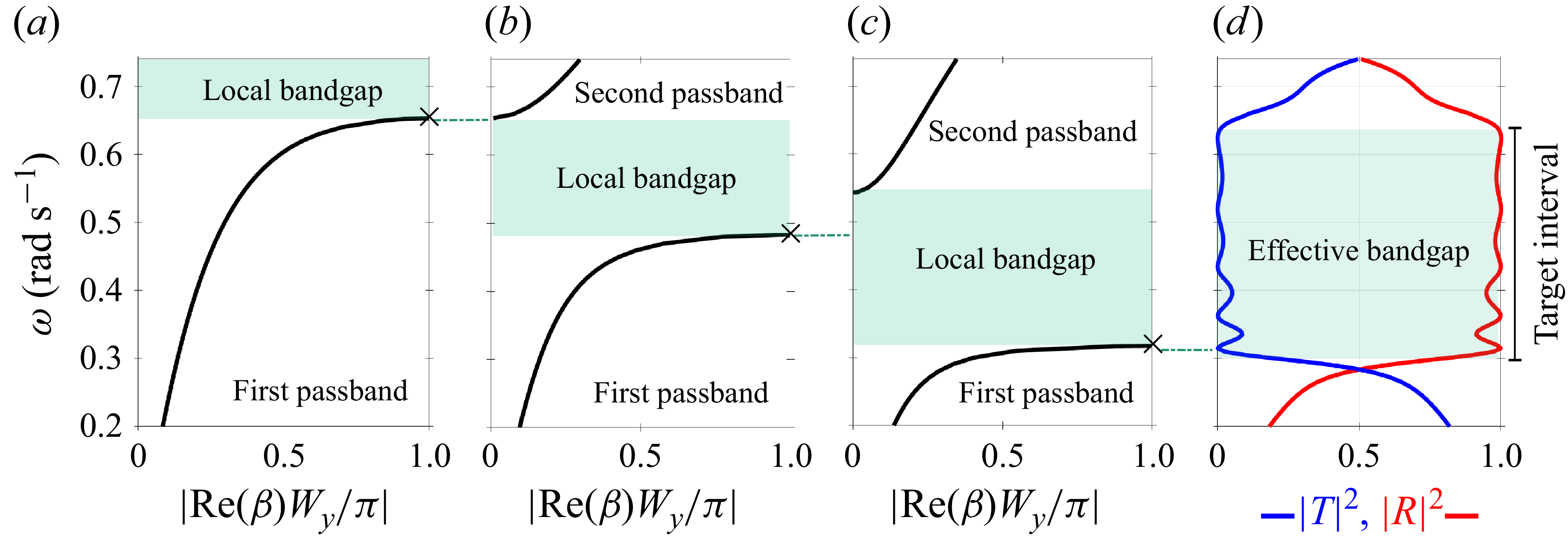
 ω0=0.65rads−1,
 ω0=0.475rads−1
 ω0=0.31rads−1
 Wx=Wy=25
 χ=π/2
 ω∈[0.3,0.65]rads−1
 |T|2≈0
 |R|2≈1

 R(ω)
 T(ω)
 ω∈C
 |R|2
 |T|2
 ω∈R
 BPTOi=0
 i=1,2,…,5

 |R|2
 α
 α
 |R|2
 |T|2
 BPTO4≠0
 |R(ω)|2≈0
 ω∈R
 Im(ω)≈0
 R(ω
 ω∈C
 Im(ω)≈0
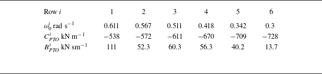
 ω0
 Wx=30
 Wy=40

 ω=0.52
 −1
 χ=π/2
 ω=0.43
 −1
 χ=π/6
 ω=0.35
 −1
 χ=π/3
 90∘

 Wx=30
 Wy=40
 ω∈[0.3,0.65]
 −1
 χ∈[π/6,π/2]

 K=5
 Wx
 Wy
 K=10
 Wx
 Wy
 Wx=30
 Wy=40

 |ζ|/Ainc
 Wx=30
 Wy=40
 ω∈[0.3,0.65]rads−1
 χ=π/2
 i
 |ζ|/Ainc
 i
 i=1,2,…,6
 j=3
 8
 j=1,2,9,10

 j=1,2,J−1,J

 (J=10)×(K=6)=60
 ω=0.52
 −1
 χ=π/2
 ω=0.35
 −1
 χ=π/3
 ω>ω03
 ω>ω05

 Hs=1
 γ=3.3
 ς=4
 Tp=10
 γ=1.54
 ς=1
 Tp=17
 (J=10)×(K=6)=60
 Wx=30
 Wy=40
 T0=10
 T0=15
 T0=20

 αspec
 γ=3.3, ς=4
 γ=1.54, ς=1
 Tp∈[9.6,20.9]
 αspec
 Tp
 T0
 Tp
 T0=Tp∈[10.3,20.9]

 Open access

