
1. Introduction
A mixture of a Newtonian fluid and high-molecular-weight polymers (even at extremely low concentration) exhibits viscoelasticity. In the low-Reynolds-number range, when the elasticity becomes the dominant source of nonlinearity, this flow can manifest many interesting and novel flow phenomena that have not been studied extensively, especially flow instabilities, such as symmetry breaking (Arratia et al. Reference Arratia, Thomas, Diorio and Gollub2006; Poole, Alves & Oliveira Reference Poole, Alves and Oliveira2007; Haward, Toda-Peters & Shen Reference Haward, Toda-Peters and Shen2018; Haward, Hopkins & Shen Reference Haward, Hopkins and Shen2020), secondary flow (Yue, Dooley & Feng Reference Yue, Dooley and Feng2008; Davoodi et al. Reference Davoodi, Lerouge, Norouzi and Poole2018), time dependency and even elastic instability and turbulence (Shaqfeh Reference Shaqfeh1996; Groisman & Steinberg Reference Groisman and Steinberg2000, Reference Groisman and Steinberg2001; Larson Reference Larson2000; Schiamberg et al. Reference Schiamberg, Shereda, Hu and Larson2006; Grilli, Vázquez-Quesada & Ellero Reference Grilli, Vázquez-Quesada and Ellero2013; Varshney & Steinberg Reference Varshney and Steinberg2019; Steinberg Reference Steinberg2021). These instability phenomena widely occur in processes ranging from plastic manufacturing (Denn Reference Denn2001; Varchanis et al. Reference Varchanis, Pettas, Dimakopoulos and Tsmopoulos2021) to human blood plasma (Brust et al. Reference Brust, Schaefer, Doerr, Pan, Garcia, Arratia and Wagner2013; Thiébaud et al. Reference Thiébaud, Shen, Harting and Misbah2014) and porous media flows (Walkama, Waisbord & Guasto Reference Walkama, Waisbord and Guasto2020; Hopkins, Haward & Shen Reference Hopkins, Haward and Shen2021). However, detailed understandings of the underlying mechanisms in many instances remain vague. In these flows, because the extra elastic stress plays a key role, it is essential to know its value and how it influences the flow field. Experimental measurement and numerical simulation are the two main approaches to obtain the elastic stress. Compared to a large number of reported experimental studies with regards to elastic instability phenomena, the numerical method is applied relatively less (Poole Reference Poole2019) to this problem and deserves to be employed more frequently because of its advantages such as more feasible parametric studies and direct analysis of the elastic stress field. However, a notoriously difficult problem in numerical simulation of viscoelastic flow has challenged researchers for decades, namely the numerical instability when simulating flow at high Weissenberg number (Wi), which is called the high-Weissenberg-number problem (HWNP). The reader is referred to the recent review paper by Alves, Oliveira & Pinho (Reference Alves, Oliveira and Pinho2021) for a more complete account of these issues. In the following, we focus on explaining an idealized flow model, that is, viscoelastic flow around a circular cylinder, and the recent studies of its upstream instability.
Viscoelastic flows past bluff bodies are frequently encountered in industrial applications (e.g. filtration processes and oil extraction) and natural phenomena (e.g. flow in soil and blood flow in cardiovascular valves and brain tissues) (Larson Reference Larson1999; Iliff et al. Reference Iliff, Wang, Liao, Plogg, Peng, Gundersen, Benveniste, Vates, Deane, Goldman, Nagelhus and Nedergaard2012; Marsden Reference Marsden2014). In addition, porous media are frequently modelled by ordered and disordered arrays of microfluidic circular cylinders (Walkama et al. Reference Walkama, Waisbord and Guasto2020; Hopkins et al. Reference Hopkins, Haward and Shen2021). Placing one or more cylinders in channel or pipe inlet section is often used as a disturbance source to study the channel viscoelastic instability in experiments (Varshney & Steinberg Reference Varshney and Steinberg2018; Qin et al. Reference Qin, Salipante, Hudson and Arratia2019b). Viscoelastic flow around a circular cylinder has also been regarded as a benchmark case for numerical and experimental studies (Ultman & Denn Reference Ultman and Denn1971; Dhahir &Walters Reference Dhahir and Walters1989). In Newtonian wake flows, a downstream recirculation zone and vortex shedding can be observed because of the global instability in these flows (Williamson & Rosirko Reference Williamson and Rosirko1988; Barkley Reference Barkley2006; Sipp & Lebedev Reference Sipp and Lebedev2007; Tang et al. Reference Tang, Yu, Shan, Li and Yu2020). However, in viscoelastic wake flows, interestingly, an upstream recirculation can form in cylinder wake flows confined between two plane plates.
The recirculation in front of a circular cylinder was firstly reported by Kenney et al. (Reference Kenney, Poper, Chapagain and Christopher2013). Later, Shi et al. (Reference Shi, Kenney, Chapagain and Christopher2015), Zhao, Shen & Haward (Reference Zhao, Shen and Haward2016), Qin et al. (Reference Qin, Salipante, Hudson and Arratia2019a), Haward et al. (Reference Haward, Hopkins, Varchanis and Shen2021) and Hopkins et al. (Reference Hopkins, Haward and Shen2022a,Reference Hopkins, Shen and Hawardb) successively studied this phenomenon experimentally. These experiments were performed using Boger solutions, which are elastic without shear thinning, such as dilute polyethylene oxide or polyacrylamide solutions, or using wormlike fluids with a strong shear-thinning behaviour, such as cationic surfactant cetyltrimethylammonium bromide and stable hydrotropic salt 3-hydroxynaphthalene-2-carboxylate solutions. Regarding the geometry of the experimental set-up, the blockage ratio (BR), i.e. the ratio of cylinder diameter to channel width, in these experiments is not less than 50 % and the depth-to-diameter ratio (α) widely ranges from 0.5 to 5. Zhao et al. (Reference Zhao, Shen and Haward2016) summarized the flow patterns in the Wi–BR space with five states: Newtonian-like state, bending streamlines, vortex growth upstream, unsteady downstream and three-dimensional time-dependent chaotic upstream, which are shown in figure 1. Qin et al. (Reference Qin, Salipante, Hudson and Arratia2019a) found that this flow is inherently three-dimensional and observed symmetry breaking as well as strong upstream propagation effects via elastic waves. At low BR (~10 %), there also exists a mild upstream instability, with only streamline bending, which was reported by Ribeiro et al. (Reference Ribeiro, Coelho, Pinho and Alves2014), Nolan et al. (Reference Nolan, Agarwal, Lei and Shields2016) and Haward et al. (Reference Haward, Toda-Peters and Shen2018). Therefore, it seems that high BR is one of the conditions for (strong) upstream instability. Besides, the experiments by Shi & Christopher (Reference Shi and Christopher2016) and Varshney & Steinberg (Reference Varshney and Steinberg2017, Reference Varshney and Steinberg2018) also showed that when the cylinders are arranged in tandem at low BR, the recirculation zone is likely to appear in the upstream region of the rear cylinders. Few studies quantitatively investigated the length of upstream recirculation. A schematic diagram of the upstream recirculation length (l) is shown in figure 2, which is the distance from the foremost end of the upstream recirculation to the foremost end of the cylinder. Using the cylinder diameter D to normalize l as LD = l/D, Zhao et al. (Reference Zhao, Shen and Haward2016) obtained a Landau-type behaviour of the dimensionless upstream recirculation length LD (LD increasing with Wi). In the experiment of Qin et al. (Reference Qin, Salipante, Hudson and Arratia2019a), LD is almost linear with the Weissenberg number based on the first normal stress difference  $W{i_N} = {N_1}/2\dot{\gamma }\eta (\dot{\gamma })$, where N 1 is the first normal stress difference,
 $\dot{\gamma }$ is the characteristic shear rate defined by the mean centreline velocity and
 $\eta (\dot{\gamma })$ is the shear viscosity at this
 $\dot{\gamma }$. It is worth pointing out that the definitions of the Weissenberg number in these two studies are different.
Summary for the Wi–BR state space of flow patterns. Panels (a, b, d), (c) and (e) are adapted from Zhao et al. (Reference Zhao, Shen and Haward2016), Hopkins et al. (Reference Hopkins, Shen and Haward2021) and Qin et al. (Reference Qin, Salipante, Hudson and Arratia2019a), respectively.

Schematic diagram of upstream recirculation length.

In the simulations of viscoelastic fluid flow, an additional elastic stress divergence term is often linearly introduced to the right-hand side of the Navier–Stokes equations. The elastic stress is closed by the constitutive relation with conformation tensor, such as upper-convected Maxwell model (Olsson & Yström Reference Olsson and Yström1993), Oldroyd-B model (Oldroyd Reference Oldroyd1950), finite extensible nonlinear elastic (FENE) model series (Herrchen & Öttinger Reference Herrchen and Öttinger1997), Phan-Thien and Tanner model (Thien & Tanner Reference Thien and Tanner1977), etc. The calculated Wi is often limited to a low value due to the aforementioned numerical instability. Varchanis et al. (Reference Varchanis, Hopkins, Shen, Tsamopoulos and Haward2020) simulated the asymmetric viscoelastic flow around a cylinder, which agreed well with their experiment. Their numerical simulation was still limited to a low BR.
Flow around a cylinder in a channel is a typical mixed flow, including shear flow and tensile flow. Using full-field time-resolved flow-induced birefringence imaging, Zhao et al. (Reference Zhao, Shen and Haward2016a) found that upstream instabilities are associated with high stress in the fluid that accelerates in the narrow gap between the cylinder surface and the channel wall when BR is large. In the narrowest area between the cylinder surface and the channel wall, the fluid parcels are strongly stretched, which results in high elastic stress there. This sharp growth in elastic stress may cause loss of convergence and trigger the well-known HWNP in numerical simulation (Hulsen, Fattal & Kupferman Reference Hulsen, Fattal and Kupferman2005). It is a challenging task to balance numerical accuracy and stability. Up to now, there have been no systematic numerical simulations to investigate this upstream flow phenomenon (Poole Reference Poole2019). In this paper, we present numerical simulations of the viscoelastic upstream instability recently observed experimentally in front of a cylinder in a narrow channel. The FENE model with the Peterlin closure (FENE-P) is adopted to describe the rheological constitutive behaviour of a dilute polymer solution. The square root reconstruction method (Balci et al. Reference Balci, Thomases, Renardy and Doering2011) is selected as the stabilization technique for the numerical simulation to handle HWNPs.
The rest of the paper is organized as follows. Section 2 introduces our specific problem, governing equations, solution method, mesh generation and grid convergence test. In § 3, we discuss our numerical results on the upstream instability. We conclude the present work in § 4. In Appendix A, we also provide more results on the validation, some additional results on the FENE-CR model, the effect of Péclet number and the effect of different boundary conditions.
2. Problem formulation and numerical method
2.1. Problem description
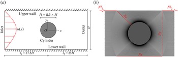
Figure 3(a) shows the computational domain, which consists of a pressure-driven flow from left to right past a circular cylinder in a confined channel. It is true that Qin et al. (Reference Qin, Salipante, Hudson and Arratia2019a) revealed the inherent three-dimensional nature of the upstream recirculation zone. However, we study the corresponding flow instability in this two-dimensional setting as the first attempt. The width of the channel is H. The diameter of the cylinder is D. Three different blockage ratios (BR = D/H), i.e. 50 %, 62.5 % and 75 %, are considered. The distance between the cylinder centre and the inlet is 37.5H (upstream region l 1) and the distance between the cylinder centre and the exit is 25H (downstream region l 2). A parabolic flow profile  $u(y) = 1.5\bar{U}(1 - 4{y^2}/{H^2})$ is adopted as the inlet velocity, where
 $\bar{U}$ is the average velocity. The zero-pressure and zero-velocity gradient conditions are adopted at the outlet. On the upper wall, the lower wall and the cylindrical wall, the no-slip boundary condition is imposed. The treatment of boundary conditions for the conformation tensor is discussed below and also in Appendix A.4.
(a) Schematic diagram of computational domain and (b) the mesh topology near the cylinder.

2.2. Governing equations
The viscoelastic fluids in the experiments of Qin et al. (Reference Qin, Salipante, Hudson and Arratia2019a,Reference Qin, Salipante, Hudson and Arratiab) and Pan et al. (Reference Pan, Morozov, Wagner and Arratia2013) show both the shear thickening of elongational viscosity and the shear thinning of shear viscosity. Thus, the FENE-P model is adopted in the present study, which takes into account the finite elongation of polymer molecules and the bounded stress. The governing equations of the flow combined with the FENE-P constitutive model read as follows (Bird, Dotso & Johnson Reference Bird, Dotso and Johnson1980; Bird, Armstrong & Hassager Reference Bird, Curtiss, Armstrong and Hassager1987):
 \begin{equation}\left. {\begin{array}{*{20}{c}} {\boldsymbol{\nabla }\boldsymbol{\cdot }\boldsymbol{u} = 0,}\\ {\rho \dfrac{{\partial \boldsymbol{u}}}{{\partial t}} + \rho (\boldsymbol{u}\boldsymbol{\cdot }\boldsymbol{\nabla })\boldsymbol{u} ={-} \boldsymbol{\nabla }p + {\eta_s}\Delta \boldsymbol{u} + \boldsymbol{\nabla }\boldsymbol{\cdot }\boldsymbol{\tau },}\\ {\dfrac{{\partial \boldsymbol{c}}}{{\partial t}} + (\boldsymbol{u}\boldsymbol{\cdot }\boldsymbol{\nabla })\boldsymbol{c} - (\boldsymbol{\nabla }\boldsymbol{u})\boldsymbol{\cdot }\boldsymbol{c} - \boldsymbol{c}\boldsymbol{\cdot }{{(\boldsymbol{\nabla }\boldsymbol{u})}^T} ={-} \dfrac{\boldsymbol{\tau }}{{{\eta_p}}},} \end{array}} \right\}\end{equation}
with
 \begin{equation}\boldsymbol{\tau } = \frac{{{\eta _p}}}{\lambda }[f(\boldsymbol{c})\boldsymbol{c} - \theta \boldsymbol{I}],\quad f(\boldsymbol{c}) = \frac{1}{{1 - tr(\boldsymbol{c})/{L^2}}}\quad \textrm{and}\quad \theta = \frac{{{L^2}}}{{{L^2} - 3}},\end{equation}
where ρ, u, p, t, λ, c, τ and I are fluid density, flow velocity, pressure, time, statistical relaxation time of polymers, conformation tensor, stress tensor of polymers and identity tensor, respectively,  $\eta _p$ and
 $\eta _s$ are the polymeric contribution to zero-shear-rate viscosity and solvent viscosity, respectively, tr denotes trace operator of tensor and the extensibility parameter L measures the maximum stretching of the polymer chains (Bird et al. Reference Bird, Dotso and Johnson1980, Reference Bird, Curtiss, Armstrong and Hassager1987; Purnode & Crochet Reference Purnode and Crochet1998). When L is set as ∞ and θ tends to 1, the FENE-P model returns to the Oldroyd-B model (Oldroyd Reference Oldroyd1950).
Note that another common FENE-type model is the FENE-CR model, which has been widely applied to predict the flow behaviour of viscoelastic fluids with a constant shear viscosity and a bounded elongational viscosity. We have also performed numerical simulations based on the FENE-CR model. More information about the FENE-CR model and a comparison of the numerical results obtained using the FENE-P model and the FENE-CR model are provided in Appendix A.3.
The main dimensionless parameters for this simulation are the Reynolds number Re and the Weissenberg number Wi, which are defined as  $Re = \rho \bar{U}H/2{\eta _0}$ and
 $Wi = 2\lambda \bar{U}/H$, respectively. It is emphasized that the present study uses the half-channel width as the reference length. Thus, a factor of 2 should be applied to the corresponding Wi defined using the whole channel width as the reference length when comparing with published data. Here
 $\eta$0 =
 $\eta_{p}$ +
 $\eta_{s}$ is the total viscosity of the solution at zero shear rate and β =
 $\eta_{s}$/
 $\eta_{0}$ is the solvent viscosity ratio, a measurement of polymer concentration and molecular characteristics of polymers. In this study, β is set to 0.59 in most of the cases. Besides, β = 0.9, 0.75, 0.45, 0.3 and 0.15 are also considered in some cases. Four values of L 2 = 400, 2500, 10 000 and 40 000 are considered. It is suggested from the definitions of Re and Wi that the fluid viscoelasticity is more prominent than the fluid inertia for microscale flows. Fluid viscoelasticity can be characterized by Wi. In this work, we mostly only change Wi to probe how the elasticity influences the upstream instability.
The drag coefficient acting on the cylinder is computed as
 \begin{equation}{C_d} = \frac{1}{{{\eta _0}\bar{U}H}}\int_S {[ - p\boldsymbol{I} + \boldsymbol{\tau } + {\eta _s}\boldsymbol{\nabla }\boldsymbol{u}]\boldsymbol{\cdot }\boldsymbol{i}\boldsymbol{\cdot }\textrm{d}\boldsymbol{S}} ,\end{equation}
where S is a vector normal to each face element of the cylinder boundary, whose magnitude is equal to the area of face element, and i is a unit vector aligned with the streamwise direction.
The fluctuation frequency (ff) of flow field and elastic stress wave in the x direction can be obtained by fast Fourier transform (FFT) of the time series of Cd. The Strouhal number St is defined as
 \begin{equation}St = {f_f}H/(2\bar{U}).\end{equation}
In the experiment of Qin et al. (Reference Qin, Salipante, Hudson and Arratia2019a) and Pan et al. (Reference Pan, Morozov, Wagner and Arratia2013), the Weissenberg number is defined using the first normal stress difference. In order to compare our numerical results with their experimental results, we calculate the first normal stress difference of the FENE-P model under simple shear flow as follows (Purnode & Crochet Reference Purnode and Crochet1998):
 \begin{align}{N_1} = \frac{{(\textrm{1}
- \beta ){\eta _0}{L^4}}}{{\lambda ({L^2} - 3)}}{\left[ \vphantom{{\Delta _1^{2/3} + \Delta
_2^{2/3} - 2{{\left(
{\frac{{2{L^6}}}{{27{\lambda^2}{{\dot{\gamma }}^2}{{({L^2}
- 3)}^2}}}} \right)}^{1/3}}}}
{\frac{{2{L^6}}}{{{\lambda^2}{{\dot{\gamma }}^2}{{({L^2} -
3)}^2}}}} \vphantom{{\Delta _1^{2/3} + \Delta
_2^{2/3} - 2{{\left(
{\frac{{2{L^6}}}{{27{\lambda^2}{{\dot{\gamma }}^2}{{({L^2}
- 3)}^2}}}} \right)}^{1/3}}}}\right]^{ - 1/3}}\left[ {\Delta _1^{2/3} + \Delta
_2^{2/3} - 2{{\left(
{\frac{{2{L^6}}}{{27{\lambda^2}{{\dot{\gamma }}^2}{{({L^2}
- 3)}^2}}}} \right)}^{1/3}}}
\right],\end{align}
where
 \begin{equation}{\Delta _1}= 1 + \sqrt {1 + \frac{{2{L^6}}}{{27{\lambda ^2}{{\dot{\gamma }}^2}{{({L^2} - 3)}^2}}}} ,\quad {\Delta _2} = 1 - \sqrt {1 + \frac{{2{L^6}}}{{27{\lambda ^2}{{\dot{\gamma }}^2}{{({L^2} - 3)}^2}}}} .\end{equation}
The shear viscosity for the special strain rate  $(\dot{\gamma })$ reads
 \begin{equation}\eta = \beta {\eta _0} + (\textrm{1} - \beta ){\eta _0}{\left[ {\frac{{{L^6}}}{{4{\lambda^2}{{\dot{\gamma }}^2}{{({L^2} - 3)}^2}}}} \right]^{1/3}}[\Delta _1^{1/3} + \Delta _2^{1/3}].\end{equation}
In experiment, the material properties of a viscoelastic fluid may be complicated and not easy to fit the parameters in the existing viscoelastic constitutive models, including the existence of branched chains of polymer molecules, the spectrum distribution of relaxation time and the certain distribution of chain lengths of polymer molecules. Herein, we use a normal stress similarity to re-calibrate the rheological parameters. The Weissenberg number based on the first normal stress difference  $W{i^{\prime}_N}$ can then be defined as the ratio of the first normal stress difference to twice the Newtonian shear stress (Qin et al. Reference Qin, Salipante, Hudson and Arratia2019a,Reference Qin, Salipante, Hudson and Arratiab), i.e.
 \begin{equation}W{i^{\prime}_N} = {N_1}/[2\dot{\gamma }(\eta - {\eta _s})],\end{equation}
which is different from Wi for the FENE-P model. The  $W{i^{\prime}_N}- Wi$ relationship for β = 0.59 is plotted in figure 4(a). For the Oldroyd-B model, L tends to infinity and we have
 \begin{equation}W{i^{\prime}_N} = Wi.\end{equation}
(a) The  $W{i^{\prime}_N}- Wi$ relationship and (b) the WiN – Wi relationship for the FENE-P model with β = 0.59.

It is worth mentioning that the above definitions for Wi and  $W{i^{\prime}_N}$ do not include the effect of β. Thus, we adopt another definition here proposed in Pan et al. (Reference Pan, Morozov, Wagner and Arratia2013):
 \begin{equation}W{i_N} = {N_1}/(2\dot{\gamma }\eta ).\end{equation}
In particular, for the Oldroyd-B model with  $L \to \infty $, one has
 \begin{equation}W{i_N} = (1 - \beta )Wi.\end{equation}
This definition reflects the influence of β. The value of WiN becomes smaller for larger β. The corresponding WiN–Wi relationship for β = 0.59 is shown in figure 4(b). Note that for β = 0.59 and L 2 = 2500, WiN is equal to 9.391 when Wi = 100, which is close to the maximum WiN in the experiments of Qin et al. (Reference Qin, Salipante, Hudson and Arratia2019a,Reference Qin, Salipante, Hudson and Arratiab) and Pan et al. (Reference Pan, Morozov, Wagner and Arratia2013).
2.3. Numerical method
The governing equations are solved by the open-source CFD platform OpenFOAM (Weller et al. Reference Weller, Tabor, Jasak and Fureby1998) and the rheoTool toolbox (Pimenta & Alves Reference Pimenta and Alves2018). Because no numerical studies have reported the upstream instability in viscoelastic wake flows, we detail our numerical method below and provide extensive validation of the numerical code. In order to ensure the boundedness of tr(c) = ckk in the FENE-P model, an implicit algorithm is used for pre-calculation before each time step (Richter, Iaccarino & Shaqfeh Reference Richter, Iaccarino and Shaqfeh2010). Tracing the transport equation of the conformation tensor yields
 \begin{equation}\frac{{\partial {c_{kk}}}}{{\partial t}} + (\boldsymbol{u}\boldsymbol{\cdot }\boldsymbol{\nabla }){c_{kk}} = tr[(\boldsymbol{\nabla }\boldsymbol{u})\boldsymbol{\cdot }\boldsymbol{c} + \boldsymbol{c}\boldsymbol{\cdot }{(\boldsymbol{\nabla }\boldsymbol{u})^T}] - \frac{{({c_{kk}} - 3){L^4}}}{{\lambda ({L^2} - {c_{kk}})({L^2} - 3)}}.\end{equation}
By defining
 \begin{equation}\varphi ={-} \ln \left( {1 - \frac{{{c_{kk}}}}{{{L^2}}}} \right),\end{equation}
equation (2.12) can be rewritten as
 \begin{equation}\frac{{\partial \varphi }}{{\partial t}} + {u_j}\frac{{\partial \varphi }}{{\partial {x_j}}} = \frac{{{e^\varphi }}}{{{L^2}}}\left( {{c_{kj}}\frac{{\partial {u_k}}}{{\partial {x_j}}} + {c_{jk}}\frac{{\partial {u_j}}}{{\partial {x_k}}}} \right) + \frac{{{e^\varphi }}}{{\lambda ({L^2} - 3)}}(3{e^\varphi } + {L^2} - {L^2}{e^\varphi }).\end{equation}
The scalar φ is solved at each time step, and then saved for the calculation of the next time step. Once φ is obtained at a given time step, the conformation tensor c can be calculated by (2.13).
Because of the high singularity of the constitutive governing equations, a small global artificial dissipation term  $\kappa \varDelta \boldsymbol{c}$ is added to the right-hand side of the transport equation of conformation tensor c in order to avoid divergence. In our simulations, we set Re = 0.0001. Molecular dissipation of polymer should be considered at this Re. The presence of this additional diffusive term can be justified by the diffusivity of polymer in solvent, which was estimated to be over the range of 10−5 to 10−7 cm2 s−1 (Haggerty, Sugarman & Prud'homme Reference Haggerty, Sugarman and Prud'homme1988). The Schmidt number Sc =
 $\eta_{0}$/ρκ, which is defined as the ratio between the zero-shear-rate viscosity and the polymer molecular diffusivity, is introduced to quantify the artificial dissipation. For dilute solution of polymer dissolved in water, the density ρ is around 1000 kg m−3. The viscosity may vary over a wide range. For example,
 $\eta_{0}$ is equal to 0.3 Pa s in the experiment of Qin et al. (Reference Qin, Salipante, Hudson and Arratia2019a). Thus, Sc is estimated over the range of 105 to 108. The normalized transport equation of conformation tensor features two dimensionless numbers, Wi and the Péclet number (Pe = Re × Sc). The value of Pe, instead of Sc, will be specified in our discussions. In the present study, Re is set to be 0.0001. The corresponding range of Pe is from 10 to 1000. The effect of Pe on the flow behaviour is discussed in Appendix A.2. By comparing the numerical results and experimental results of Qin et al. (Reference Qin, Salipante, Hudson and Arratia2019a), Pe is fixed at 40 for the final simulation.
In order to improve the stability of numerical calculation, a stabilization technique must be adopted. More information on common stabilization techniques can be found in Appendix A.1. We perform a preliminary study to test two stabilization techniques, i.e. the logarithmic reconstruction method and the square root reconstruction method. In the numerical results based on the logarithmic reconstruction method, we do not observe the upstream recirculation found in the experiments of Qin et al. (Reference Qin, Salipante, Hudson and Arratia2019a). Moreover, the logarithmic reconstruction method was also adopted by Mokhtari et al. (Reference Mokhtari, Latché, Quintard and Davit2022) and Kumar & Ardekani (Reference Kumar and Ardekani2022) and the upstream recirculation was not reported in their simulations. However, the square root reconstruction method can successfully predict the upstream recirculation, which is, therefore, adopted in the present simulation. A new symmetric tensor b is introduced satisfying  $\boldsymbol{c} = \boldsymbol{b}\boldsymbol{\cdot }{\boldsymbol{b}^T}$. The transport equation of conformation tensor c can then be rewritten as
 \begin{equation}\frac{{\partial \boldsymbol{b}}}{{\partial t}} + (\boldsymbol{u}\boldsymbol{\cdot }\boldsymbol{\nabla })\boldsymbol{b} = \boldsymbol{b}\boldsymbol{\nabla }\boldsymbol{u} + \boldsymbol{ab} + \frac{1}{{2\lambda }}(\theta \boldsymbol{\cdot }{({\boldsymbol{b}^T})^{ - 1}} - \boldsymbol{b}{e^\varphi }) + \frac{\kappa }{2}\Delta \boldsymbol{b} + \kappa \boldsymbol{h},\end{equation}
where
 \begin{equation}\boldsymbol{h} = {\boldsymbol{b}^{ - 1}}[{\textstyle{1 \over 2}}(\Delta \boldsymbol{b})\boldsymbol{b} + {({\partial _x}\boldsymbol{b})^2} + {({\partial _y}\boldsymbol{b})^2} + {({\partial _z}\boldsymbol{b})^2}].\end{equation}
As advised by Balci et al. (Reference Balci, Thomases, Renardy and Doering2011), the term  $\kappa \boldsymbol{h}$ in (2.15) is ignored in our numerical study. Note that a in (2.15) is an antisymmetric tensor, which can be written in the form of components as
 \begin{equation}\boldsymbol{a}= \left( {\begin{array}{*{20}{@{}c@{}}} 0&{{a_{12}}}&{{a_{13}}}\\ { - {a_{12}}}&0&{{a_{23}}}\\ { - {a_{13}}}&{ - {a_{23}}}&0 \end{array}} \right).\end{equation}
The components of a can be calculated by solving the following equations:
 \begin{equation}\left. {\begin{array}{*{20}{c@{}}} {({b_{11}} + {b_{22}}){a_{12}} + {b_{23}}{a_{13}} - {b_{31}}{a_{23}} = {w_1},}\\ {{b_{23}}{a_{12}} + ({b_{11}} + {b_{33}}){a_{13}} + {b_{12}}{a_{23}} = {w_2},}\\ { - {b_{13}}{a_{12}} + {b_{12}}{a_{13}} + ({b_{22}} + {b_{33}}){a_{23}} = {w_3},} \end{array}} \right\}\end{equation}
where
 \begin{equation}\left. {\begin{array}{*{20}{c@{}}} {{w_1} = ({b_{12}}{u_{1,1}} - {b_{11}}{u_{2,1}}) + ({b_{22}}{u_{1,2}} - {b_{12}}{u_{2,2}}) + ({b_{23}}{u_{1,3}} - {b_{13}}{u_{2,3}}),}\\ {{w_2}= ({b_{13}}{u_{1,1}} - {b_{11}}{u_{3,1}}) + ({b_{33}}{u_{1,3}} - {b_{13}}{u_{3,3}}) + ({b_{23}}{u_{1,2}} - {b_{12}}{u_{3,2}}),}\\ {{w_3} = ({b_{13}}{u_{2,1}} - {b_{12}}{u_{3,1}}) + ({b_{23}}{u_{2,2}} - {b_{22}}{u_{3,2}}) + ({b_{33}}{u_{2,3}} - {b_{23}}{u_{3,3}}).} \end{array}} \right\}\end{equation}
Here ui ,j are the components of  $\boldsymbol{\nabla }\boldsymbol{u}$. For a detailed description of this method, the reader is referred to Balci et al. (Reference Balci, Thomases, Renardy and Doering2011).
The second-order backward scheme is used for time discretization. The time step Δt in our simulation is set small enough to ensure numerical stability. The MINMOD scheme is adopted for discretization of  $\boldsymbol{u}\boldsymbol{\cdot }\boldsymbol{\nabla }\boldsymbol{b}$. The second-order upwind scheme is adopted for discretization of
 $\boldsymbol{u}\boldsymbol{\cdot }\boldsymbol{\nabla }\boldsymbol{u}$. For the tensor b, the linear extrapolation boundary with second-order accuracy is imposed on the upper and lower walls, and no-flux boundary condition with first-order accuracy on the cylindrical wall, to ensure the stability of numerical calculation. More discussion on the boundary condition for the tensor b can be found in Appendix A.4. The pUcoupled algorithm is adopted for the pressure–velocity coupling (Jareteg Reference Jareteg2012; Pimenta & Alves Reference Pimenta and Alves2019). Our simulation is performed using the rheoFoam solver module of rheoTool in OpenFOAM extend 4.0 (Pimenta & Alves Reference Pimenta and Alves2018). The validation of the present numerical method is provided in Appendix A.1.
The subcritical bifurcation can be distinguished by checking whether the simulation result is path-dependent or not, as shown in figure 5. In the present study, we systematically vary the controlling parameter Wi and the initial condition to examine their effects on the final simulation result. In the increasing Wi process, we gradually and slowly increase Wi and use the numerical result of the current state to initialize the simulation for the next simulation. In the decreasing Wi process, we gradually and slowly decrease Wi and use the numerical result of the current state to initialize the simulation for the next state. We explicitly point out which process is applied to perform the simulation only if the results at the same Wi obtained for the increasing and decreasing Wi processes are not identical. For an instability indicator A around the linear critical condition (Wic, as shown in figure 5), finite-amplitude solutions can exist even if Wi is less than Wic, which results in a different increasing Wi path from a decreasing Wi path (the hysteresis phenomenon). This method for identifying subcritical bifurcation has been widely used in previous studies (Becherer, Morozov & van Saarloo Reference Becherer, Morozov and van Saarloo2009; Pan et al. Reference Pan, Morozov, Wagner and Arratia2013; Burshtein et al. Reference Burshtein, Zografos, Shen, Poole and Hawar2017). In this paper, LD, the root-mean-square upstream recirculation length RMS(LD), the time-averaged drag coefficient  $\overline {{C_d}} $, the root-mean-square drag coefficient Cdrms and an asymmetry parameter I (defined in (3.8)) are selected as the instability indicators.
Method to identify subcritical bifurcation. The solid and dashed lines denote the stable and unstable solutions, respectively. Parameter Wic denotes the critical condition; IW and DW denote the increasing and decreasing Wi processes, respectively.

2.4. Mesh generation and grid convergence test
A block-structured mesh is generated for the computational domain using the commercial software ANSYS ICEM. The surrounding region of the cylinder is discretized by an O-type mesh, as shown in figure 3(b). The remainder of the computational domain is discretized using several blocks of quadrilateral meshes. In the y direction, Ny = 121 (for BR = 50 %, 201 for BR = 65 % and 75 %) grid points are unevenly distributed. In the x direction, Nx = Ny. The dense mesh is applied near the cylinder. The O-type mesh comprises Ns = 2(Nx + Ny − 2) = 800 (BR = 65 % and 75 %) or 440 (BR = 50 %) grid points uniformly distributed along the cylinder perimeter and Nr = 200 (BR = 65 % and 75 %) or 120 (BR = 50 %) grid points stretched over an exponential progression along the radial direction to ensure a fine mesh near the cylinder surface. We set the first cell side-by-side to the cylinder surface in the radial direction to 0.00125H. In the x direction, Nl 1 = 701 grid points are set in the upstream region, and Nl 2 = 301 grid points are unevenly arranged in the downstream region. In the y direction, Ny = 121 (201 for BR = 65 % and 75 %) grid points are unevenly distributed. The total number of cells in the computational domain is approximately 280 000 (BR = 65 % and 75 %) or 150 800 (BR = 50 %). The detailed mesh generation description can be found in our previous publication (Peng et al. Reference Peng, Li, Xiong, Xu and Yu2021).
The parameter set (BR, Wi, L 2, β) = (50 %, 30, 2500, 0.59) is selected to check the mesh dependency and the corresponding simulation is performed on three sets of meshes, which are listed in table 1. The effect of the mesh size on LD is investigated. In our numerical simulation, LD is measured as the horizontal distance from the most remote upstream stagnation point (u = 0 and v = 0) to the front end of the cylinder. The simulation results show that LD for Mesh1 is time dependent and its variation range is recorded in table 1. Length LD is steady for Mesh2 and Mesh3 and the difference between the results for Mesh2 and Mesh3 is 3 %. We thus consider that our numerical results for Mesh2 are accurate enough and the final simulations are performed on this mesh.
Parameter set (BR, Re, Wi, L 2, β) = (50 %, 0.0001, 30, 2500, 0.59). Here  $N{l_1}$ and
 $N{l_2}$ denote the grid numbers of the upstream and downstream regions along the x direction, respectively; Nx and Ny denote the grid numbers in the x and y directions, respectively; Nr denotes the grid numbers radiating from the cylinder surface; and
 $\Delta r$ is the grid size of the innermost grid near the cylinder wall.

3. Results and discussion
In this section, we report the numerical results of the viscoelastic wake flow in a confined channel. The parameters considered are (BR, β) = (50 %, 0.59) and L 2 = 400, 2500, 10 000 or 40 000 in § 3.1; β = 0.59, L 2 = 400, 2500, 10 000 or 40 000 and BR = 10 % to 75 % to study the effect of BR in § 3.2; and BR = 50 % or 75 %, L 2 = 2500 or 10 000 and β = 0.1–0.9 to study the effect of β in § 3.3. Table 2 summarizes the parameter space of the present study. In a certain parameter range, the flow is unsteady. We use the data in five statistical cycles to calculate the time-averaged power spectral density (PSD) and urms quantities after the flow reaches the statistically steady state.
Parameter space of the present study.

Before we perform the flow simulations, the effect of the length of downstream region l 2 on the upstream recirculation is examined. Here we consider the parameter set (BR, β, L 2, Wi) = (50 %, 0.59, 2500, 60). Three different l 2 of 25H, 50H and 100H are investigated. The upstream recirculation lengths at different l 2 are summarized in table 3, which indicates that l 2 has a very small effect on the upstream recirculation. To save computational time, l 2 = 25H is selected for the final simulation.
Effect of l 2 on the upstream recirculation length.

3.1. High-Weissenberg-number simulations for the FENE-P model at BR = 50 %
Simulation is first performed for the case with the parameter set (BR, β, L 2) = (50 %, 0.59, 2500). The set (BR, β) = (50 %, 0.59) is often used as a benchmark case for numerical simulation. Due to the numerical instability and heavy calculation burden, Wi was often set to less than 0.5 in previous studies (e.g. Fan, Tanner & Phan-Thien Reference Fan, Tanner and Phan-Thien1999; Alves, Pinho & Oliveira Reference Alves, Pinho and Oliveira2001; Hulsen et al. Reference Hulsen, Fattal and Kupferman2005). In our numerical simulation, relatively high-Wi flows (up to 100) are calculated by considering polymer molecular diffusion and using a small time step. Lee, Hwang & Cho (Reference Lee, Hwang and Cho2021) indicated that the effect of molecular dissipation of polymer can be negligible only when Pe is large (Pe > ~105) and Wi is small (Wi < ~1). Since the maximum Wi considered is 100 and Pe is equal to 40 in the present study, molecular dissipation of polymer should be taken into account.
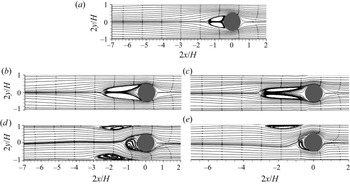
The streamline distributions and the u velocity profiles are shown in figure 6. In a Newtonian fluid, the flow is almost symmetric with respect to the cylinder as shown in figure 6(a). As Wi increases, the velocity decreases gradually along the directions approaching the cylinder both upstream and downstream, and the downstream velocity decreases faster. Figure 6(f) indicates that the downstream u velocity almost linearly increases with x except for the region near the cylinder wall for different Wi, which is consistent with the experimental results of Haward et al. (Reference Haward, Toda-Peters and Shen2018). Note that the strain rate at the rear stagnation point of the cylinder is equal to zero (Haward et al. Reference Haward, Kitajima, Toda-Peters, Takahashi and Shen2019). At Wi = 15, a recirculation zone starts to form upstream of the cylinder. Correspondingly, a region of negative u velocity can be observed in the upstream recirculation region as shown in figure 6(f). With a further increase in Wi, the upstream recirculation bubble becomes larger.
Streamlines for Newtonian (a) and viscoelastic (b–e) fluids at BR = 50 %, β = 0.59 and L 2 = 2500 for different Wi and the corresponding u velocity profiles along y = 0 (f). The contours in (a–e) are coloured by  $\sqrt {{u^2} + {v^2}} /\bar{U}$. All the streamlines are almost symmetric about the horizontal centreline of the cylinder.

To better understand the upstream recirculation, we follow Lee et al. (Reference Lee, Dylla-Spears, Teclemariam and Muller2007) and discuss the flow-type parameter defined as
 \begin{equation}\xi (x,y) = \frac{{|\dot{\boldsymbol{\gamma }}|- |\boldsymbol{\varOmega }|}}{{|\dot{\boldsymbol{\gamma }}|+ |\boldsymbol{\varOmega }|}},\end{equation}
where  $|\dot{\boldsymbol{\gamma }}|= \sqrt {{\textstyle{1 \over 2}}\boldsymbol{D}:\boldsymbol{D}}$ and
 $|\boldsymbol{\varOmega }|= \sqrt {{\textstyle{1 \over 2}}\boldsymbol{\varOmega }:\boldsymbol{\varOmega }}$ are the magnitudes of the deformation rate tensor
 $\boldsymbol{D} = {\textstyle{1 \over 2}}(\boldsymbol{\nabla }\boldsymbol{u} + \boldsymbol{\nabla }{\boldsymbol{u}^T})$ and the vorticity tensor
 $\boldsymbol{\varOmega } = {\textstyle{1 \over 2}}(\boldsymbol{\nabla }\boldsymbol{u} - \boldsymbol{\nabla }{\boldsymbol{u}^T})$, respectively, which can be locally evaluated using the components of the velocity vectors. Parameter ξ is all-coordinate invariant (Lee et al. Reference Lee, Dylla-Spears, Teclemariam and Muller2007). Here, ξ = −1 indicates solid body rotation, ξ = 0 simple shear and ξ = 1 pure extension. The flow strength in the extensional regions is quantified by the principal strain rate or the eigenvector of D (Astarita Reference Astarita1979):
 \begin{equation}{\lambda _1} = {\textstyle{1 \over 2}}\sqrt {{{({D_{11}} - {D_{22}})}^2} + 4D_{12}^2} .\end{equation}
In order to better describe the tensile strength in the extension area, a dimensionless parameter λ 2 is defined by multiplying λ 1 and ξ:
 \begin{equation}{\lambda _2} = \xi {\lambda _1}.\end{equation}
A local stretch Weissenberg number is defined as
 \begin{equation}Wi_{local}^{elastic} = \frac{\lambda }{{{u^2} + {v^2}}}\left[ {{u^2}\frac{{\partial u}}{{\partial x}} + uv\frac{{\partial v}}{{\partial x}} + uv\frac{{\partial u}}{{\partial y}} + {v^2}\frac{{\partial v}}{{\partial y}}} \right],\end{equation}
which describes the local effect on the Weissenberg number caused by stretching (positive  $Wi_{local}^{elastic}$) or compression (negative
 $Wi_{local}^{elastic}$) of fluid parcels along the flow streamline direction.
The ξ and λ 2 distributions are shown in figures 7(a) and 7(b), respectively. In a Newtonian fluid, both ξ and λ 2 distribute symmetrically against the x and y axes with respect to the cylinder. The fluid parcel around the cylinder exhibits high extension. Just upstream of the cylinder, the flow velocity is reduced, resulting in compression. In the narrow gap between the cylinder surface and the channel wall with x < 0, flow velocity increases, resulting in stretching. Figure 7 shows that the upstream compression or stretching regions further expand upstream along the middle line (y = 0) and the gap middle line (y = 3/8H) as Wi increases. The λ 2 distribution demonstrates that the strongest tensile strength region appears in the gap between the cylinder surface and the channel wall.
(a) Flow-type parameter distributions and (b) dimensionless λ 2 distributions.

The local elastic stretch Weissenberg numbers  $(Wi_{local}^{elastic})$ at y = 0 and y = 3/8H are extracted and shown in figure 8. As defined above, positive and negative
 $Wi_{local}^{elastic}$ denote fluid stretching and compression, respectively. At y = 0, the initial decrease in the flow velocity results in a negative
 $Wi_{local}^{elastic}$ for a long distance. Parameter
 $Wi_{local}^{elastic}$ initially decreases and then increases along the x direction. Generally, the location of the valley point moves upstream and the corresponding minimum
 $Wi_{local}^{elastic}$ decreases with increasing Wi. For Wi = 60, the minimum
 $Wi_{local}^{elastic}$ is about −19.8. At y = 3/8H, the increase in the flow velocity results in a positive
 $Wi_{local}^{elastic}$ for a long distance. Before approaching 2x/H = 0, Wi rapidly increases to the peak value and then experiences a sudden drop. The maximum
 $Wi_{local}^{elastic}$ is about 68.1 for Wi = 60, which occurs in the gap between the cylinder surface and the channel wall. The absolute
 $Wi_{local}^{elastic}$ in the gap (= 68.1) is much larger than that in front of the cylinder (= 19.8). The large
 $Wi_{local}^{elastic}$ in the gap reflects that the high elastic stress is concentrated there, which extends upstream near the wall region as shown in figure 9. A similar observation has been reported by Zhao et al. (Reference Zhao, Shen and Haward2016) in wormlike fluids.
Variation of the local elastic stretch Weissenberg number along the x direction at (a) y = 0 and (b) y = 3/8H.

Contours of  $1/(1 - {c_{kk}}/{L^2})$ for different Wi;
 $1/(1 - {c_{kk}}/{L^2})$ is positively correlated with the elastic stress.

A well-known dimensionless parameter which rationalizes these streamline instabilities is the M parameter introduced by McKinley, Pakdel & Öztekin (Reference McKinley, Pakdel and Öztekin1996):
 \begin{equation}M = {\left[ {\frac{{\lambda \bar{U}}}{\Re }\frac{{{\tau_{11}}}}{{({\eta_0}|\dot{\boldsymbol{\gamma }}|)}}} \right]^{1/2}},\end{equation}
where  $\lambda \bar{U} = l$ is the characteristic length over which perturbations to the base stress and velocity fields relax,
 $\Re$ is the streamline radius of curvature and
 ${\tau _{11}}$ is the streamwise tensile stress. We convert this definition of the criterion to a form amenable to local evaluation in flows by the substitution of characteristic values with local values. To consider local effective relaxation time
 $({\lambda _{eff}} = \lambda /f)$ and ignore solid-like rotational flows, Cruz et al. (Reference Cruz, Poole, Afonso, Pinho, Oliveira and Alves2016) proposed a modified Pakdel–McKinley criterion:
 \begin{equation}{M^\ast } = {\left[ {\frac{{{\lambda_{eff}}|\boldsymbol{u}|}}{r}\frac{{{\tau_{11}}}}{{||\boldsymbol{\tau }|{|_F}}}} \right]^{1/2}},\end{equation}
where  $r = |\boldsymbol{u}{|^3}/|\boldsymbol{u} \times \boldsymbol{\dot{u}}||$. Here we note that
 $\dot{\boldsymbol{u}}$ is the material derivative of the velocity vector, which is equivalent to
 $\boldsymbol{u}\boldsymbol{\cdot }\boldsymbol{\nabla }\boldsymbol{u}$ for steady-state flow. The Frobenius norm
 $(||\cdot |{|_F})$ is used, so that the resulting
 ${\tau _{11}}/||\boldsymbol{\tau }||_F$ will vary between zero, when the normal stress is weak, and one, when the tensile normal stress dominates, in highly elastic shear or extensional flows. Therefore in strongly extensional flows, M* is approximately given by
 ${\lambda _{eff}}|\boldsymbol{u}|/r$.
Contours of M* for different Wi are shown in figure 10. The largest M* region occurs in the gap between the cylinder and the outer wall. In the upstream recirculation regions, we can also find non-negligible, though smaller, values of M*. From the definition of M*, high M* happens in highly elastic shear or extensional flows. Although the flow curvature in the recirculation zone is large, we only see a relatively small value of M* in the recirculation region because the extension in this region is not larger than that in the gap regions (figure 8). The distribution of M* suggests that the instability is most likely related to the high-shear region near the cylinder, which could be classified as the standard curve-streamline shear flow instability. This conclusion would be also consistent with that reported in Davoodi, Dominques & Poole (Reference Davoodi, Dominques and Poole2019) where the effect of strain rate on the start point of purely elastic instability in elongational-dominated flows was investigated.
Contours of M* in the viscoelastic cylindrical wake flow with upstream instability for different Wi.

The above results indicate that  $Wi_{local}^{elastic}$ and the stress dominate in the gap, compared with those in front of the cylinder. In this sense, the flow across the gap can be regarded as a main flow, while the upstream recirculation is a secondary flow. A primary–secondary flow model shown in figure 11 can be applied to characterize this upstream recirculation, i.e. a high-speed stretching gap flow and a relatively low-speed upstream recirculation.
The primary–secondary flow model for the present flow configuration.

The time evolutions of the drag coefficient for Wi = 70, 80, 90 and 100 are plotted in figure 12. To save computing time, the numerical result of Wi = 60 (at time of  $2t\bar{U}/H = 525$) is set as the initial value for these higher-Wi flows. The drag acting on the cylinder increases with Wi when Wi > ~0.5 (refer to data in table 5 for low-Wi range and data here in high-Wi range), no matter whether the flow is steady (Mokhtari et al. Reference Mokhtari, Latché, Quintard and Davit2022) or unsteady. The time-averaged drag coefficient
 $(\overline {{C_d}} )$ is ~532 at Wi = 80 but ~799 at Wi = 82.5. A sharp increase in
 $\overline {{C_d}} $ is observed when Wi increases from 80 to 82.5 as shown in figure 12(a), which results from the enhancement in the additional extensional viscosity due to flow fluctuations (Browne & Datta Reference Browne and Datta2021) as shown in figure 12(b). A similar sudden increase of drag was also reported in the numerical simulation of Grilli et al. (Reference Grilli, Vázquez-Quesada and Ellero2013). Therefore, the increase in
 $\overline {{C_d}} $ with increasing Wi is sharper in unsteady flow than in steady flow.
The solid black lines denote the temporal histories of the drag coefficient at (BR, β, L 2) = (50 %, 0.59, 2500) for (a) Wi = 70, (b) Wi = 80, (c) Wi = 90 and (d) Wi = 100. The dashed brown line in (d) denotes the temporal history of LD.

When Wi < ~80, our calculation indicates that the flow is steady after developing for a long time. However, the flow becomes unsteady when Wi ≥ 80. At Wi = 80, the fluctuation of drag coefficient exhibits a fully developed periodic state with a single frequency demonstrated by the FFT analysis shown in figure 13(a). For Wi = 100 in figure 12(d), the variation of drag coefficient roughly maintains a periodic state that features more discrete frequencies demonstrated by the FFT analysis shown in figure 13(b). Interestingly, the quantitative analysis demonstrates St 4 ≈ 4St 1, St 3 ≈ 3St 1 and St 2 ≈ 2St 1, indicating the nonlinear effect of the period-doubling. Figure 12(d) also shows the corresponding time evolution of LD for one period, which exhibits a trend similar to that of the Cd curve. The maximum drag of the cylinder corresponds to the longest upstream recirculation. The corresponding streamlines at four time instants within one period are shown in figure 14.
The FFT of the drag coefficients for (BR, β, L 2) = (50 %, 0.59, 2500) at (a) Wi = 80 and (b) Wi = 100.

Streamlines at time instants (a) t = t 1, (b) t = t 2, (c) t = t 3 and (d) t = t 4 marked in figure 12(d) for (BR, β, L 2, Wi) = (50 %, 0.59, 2500, 100).

A sharp increase of drag between Wi = 80 and 82.5 under the increasing Wi process (i.e. the discontinuity on the  $\overline {{C_d}} - Wi$ curve near Wi = 82.5) shown in figure 15(a) implies a subcritical transition. We use the result of Wi = 82.5 as the initial field to study this transition behaviour and gradually reduce Wi (i.e. the decreasing Wi process). It is found that the
 $\overline {{C_d}} - Wi$ curve maintains continuity until Wi = 67.5 and then experiences a sudden drop between Wi = 67.5 and 65 as shown in figure 15(a). Both figures 15 and 16 show that the unsteady flow becomes steady when Wi is decreased from Wi = 67.5 to Wi = 65. The hysteresis phenomenon shown in figure 15(b) implies that the transient transition is a subcritical Hopf bifurcation.
Variations of (a) the time-averaged drag coefficient  $(\overline {{C_d}} )$ and (b) the root-mean-square drag coefficient (Cdrms) with Wi for (BR, β, L 2) = (50 %, 0.59, 2500). Here IW and DW denote the increasing and decreasing Wi processes, respectively.

The temporal histories of the drag coefficient at (BR, β, L 2) = (50 %, 0.59, 2500) for (a) Wi = 67.5 and (b) Wi = 65 under the decreasing Wi process. The numerical result of Wi = 82.5 is selected as the initial field. Here DW denotes the decreasing Wi process.

For L 2 = 10 000 and 40 000, we also observe the upstream recirculation. The non-dimensional recirculation length (LD) as a function of Wi for L 2 = 2500, 10 000 and 40 000 is summarized in figure 17(a). At high Wi, the flow becomes unsteady for L 2 = 2500, as discussed above. For L 2 = 40 000, the flow also becomes unsteady when Wi ≥ 70. However, for L 2 = 10 000, the unsteady behaviour is only observed when 20 ≤ Wi ≤ 50. When the flow is unsteady and LD varies with time, the maximum and minimum values of LD at the corresponding Wi are provided, as shown in figure 17(a). Note that we only present the result up to Wi = 60 for L 2 = 40 000 here. A further increase in Wi causes simulation divergence due to numerical instability, even if we use a very small time step. We observe a sudden increase of LD before simulation divergence.
(a) The LD–Wi relationship and (b) the LD–WiN relationship at (BR, β) = (50 %, 0.59). When the flow becomes unsteady and LD varies with time at high Wi, the time-averaged LD is provided while the error bar indicates the corresponding maximum and minimum values. Here IW and DW denote the increasing and decreasing Wi processes, respectively.

Length LD for L 2 = 40 000 is shorter than those for L 2 = 2500 or L 2 = 10 000. However, Qin et al. (Reference Qin, Salipante, Hudson and Arratia2019a) implies the upstream recirculation length is positively correlated with extensional viscosity. Variation of LD with WiN is plotted in figure 17(b). As mentioned above, the definition of WiN is similar to that in Pan et al. (Reference Pan, Morozov, Wagner and Arratia2013). The time-averaged LD measured by Qin et al. (Reference Qin, Salipante, Hudson and Arratia2019a) is also plotted in figure 17(b). Behaviour of LD at L 2 = 2500 is mostly consistent with the experimental results of Qin et al. (Reference Qin, Salipante, Hudson and Arratia2019a). It is worth pointing out that in their experiment, the upstream recirculation length varies strongly with time when WiN is beyond 4.35. However, the fluctuation of LD is not very obvious in our simulation when WiN > 13.5 for L 2 = 10 000. Note that the present simulation is two-dimensional and the present rheological model and parameters may be different from those for the material used in the experiment. Besides, Re may be different between our simulation and their experiment. Thus, the temporal behaviour of LD deviates from that reported by Qin et al. (Reference Qin, Salipante, Hudson and Arratia2019a).
Figure 17 clearly shows that there is a critical Weissenberg number Wic for the onset of the upstream recirculation at each L 2. Close to the transition, LD increases smoothly from zero to a non-zero value with increasing Wi, and the relationship between LD and Wi can be well described by a simple Landau-type quartic potential minimized as
 \begin{equation}Wi = W{i_c}(gL_D^2 + hL_D^{ - 1} + 1),\end{equation}
where g denotes the growth rate coefficient and h quantifies system imperfection that biases a transition to a favoured branch. Figure 18 shows the relationship between LD and Wi for both the numerical results and the fitted data around the onset of the upstream recirculation region. The corresponding values of g and h are listed in table 4. The fitted Wic and g increase with L 2 while h is always close to zero. When L 2 = 10 000, the fitted curve only collapses well with the numerical results when Wi is less than 40. This implies that at BR = 50 %, variation in Wi may cause inherent change in flow state when L 2 = 10 000. It may result from the velocity increase in the gap between the cylinder surface and the channel wall. The time-averaged streamlines and contours of the dimensionless u velocity for Wi = 40 and 50 are shown in figures 19(a) and 19(b). The streamlines indicate that the upstream recirculation elongates when Wi increases from 40 to 50. Meanwhile, the contours of the dimensionless u velocity show that the maximum velocity in the gap between the cylinder surface and the channel wall increases from 3.31 at Wi = 40 to 3.65 at Wi = 50. The maximum time-averaged dimensionless x-direction velocity in the flow field  $\textrm{max(}\bar{u}/\bar{U})$ is extracted and plotted in figure 19(c). Obviously, a significant increase in velocity occurs between Wi = 40 and 50. At high Wi, the elastic stress is concentrated near the channel and cylinder walls, which acts to narrow the gap and accelerate the flow velocity there. For example, the maximum velocity in the gap is 3.65 for (Wi, L 2) =(50, 10 000); however, it is about 3 for a Newtonian fluid. The effect of BR on the upstream recirculation is discussed in the next section.
Variation of LD with Wi at BR = 50 % for (a) L 2 = 400, (b) L 2 = 2500, (c) L 2 = 10 000 and (d) L 2 = 40 000. The solid line denotes the data fitted with Landau-type quartic potential while the symbols  $\bullet$, ♦, ★ and
 $\ast$ denote the numerical results. The fitted Wic for each L 2 is summarized in table 4. Here IW and DW denote the increasing and decreasing Wi processes, respectively.

Time-averaged flow streamlines and contours of the dimensionless u velocity at (BR, β, L 2) = (50 %, 0.59, 10 000) for (a) Wi = 40 and (b) Wi = 50. (c) Variation of the maximum time-averaged dimensionless u velocity  $\textrm{max}(\bar{u}/\bar{U})$ with Wi.

The fitting parameters for BR = 50 % in (3.7).

3.2. Effect of BR on viscoelastic upstream instability
Previous experiments indicated that the upstream recirculation occurs when BR is not less than 50 %. When BR is low, such as 10 %, only upstream streamline bending occurs (Haward et al. Reference Haward, Toda-Peters and Shen2018). Thus, there is a critical value of BR which is around 50 % and determined by Wi and L 2, below which the upstream recirculation will not occur. When BR is 50 % and Wi is low in the simulations discussed in § 3.1, the velocity in the midline (y = 0) changes from 1.5 at the inlet to 0 at the cylinder surface, which results in a compression  $Wi_{local}^{elastic}$. However, the velocity along y = 3/8H changes from about 1.5 at the inlet to about 3.0 in the gap, which leads to a stretching
 $Wi_{local}^{elastic}$. The maximum compression
 $Wi_{local}^{elastic}$ is almost equal to the maximum stretching
 $Wi_{local}^{elastic}$ in this situation. When BR exceeds 50 %, the gradient of flow velocity in the gap is steeper than that upstream of the cylinder. That is, the stretching
 $Wi_{local}^{elastic}$ upstream is larger than the compression
 $Wi_{local}^{elastic}$ in the gap. The compression
 $Wi_{local}^{elastic}$ in the gap plays a leading role, which results in a primary–secondary flow as shown in figure 11. Moreover, with the increase of Wi, the flow velocity inside the gap may slightly increase (discussed in last paragraph in § 3.1). This indicates that the blockage effect is more severe and the apparent BR is increased (the increase of the flow rate in the centreline of the gap can be equivalent to the increase of BR). Therefore, the upstream recirculation also occurs when BR = 50 %.
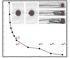
It is reasonable to speculate that a certain boundary exists in the space of (BR, Wi) to distinguish the regimes with and without the upstream recirculation. Thus, we studied the effect of BR on Wic for (β, L 2) = (0.59, 2500), as shown in figure 20. Note that Wi does not exceed 100 in this test. Here Wic is not obtained by fitting (3.7). Instead, at a given BR, multiple simulations are performed near Wic. The bisection method is adopted to determine Wic by checking whether the upstream recirculation occurs. Our results imply that the upstream recirculation only occurs when BR is more than 16.7 %, i.e. the Wi c–BR curve asymptotically approaches BR ~ 16.7 %. Hopkins et al. (Reference Hopkins, Haward and Shen2022a) found that for a viscoelastic wormlike micellar solution, the upstream recirculation is observed only when BR is greater than certain thresholds and Wic is almost inversely proportional to BR. Our numerical simulation results qualitatively agree with their experimental results. We also select five typical cases with (BR, Wi) = P 1 (25 %, 20), P 2 (25 %, 30), P 3 (50 %, 20), P 4 (62.5 %, 20) and P 5 (75 %, 20) to demonstrate the instantaneous streamlines. Here P 1 is under the Wic–BR curve and no upstream recirculation exists. In contrast, P 2 to P 5 are all located above the Wic–BR curve, and the upstream recirculation does occur. For a fixed Wi, as BR increases (P 3, P 4 and P 5), the upstream recirculation becomes longer and behaves asymmetrically. This asymmetric behaviour is explained later in this section.
Variation of Wic with BR for (β, L 2) = (0.59, 2500). The instantaneous streamlines for five typical cases with (BR, Wi) = P 1 (25 %, 20), P 2 (25 %, 30), P 3 (50 %, 20), P 4 (62.5 %, 20) and P 5 (75 %, 20) are plotted.

In the rest of this subsection we mainly consider high BR of 62.5 % and 75 % and discuss its effect on the upstream recirculation. Figures 21(a) and 21(b) plot LD as a function of Wi for BR = 62.5 % and 75 %, respectively. When (BR, L 2) = (62.5 %, 2500), (62.5 %, 10 000), (75 %, 400) and (75 %, 2500), the growth of upstream recirculation with Wi close to the transition also satisfies (3.7), as shown in figures 22(a,b) and 23(a,b). However, when (BR, L 2) = (62.5 %, 40 000), (75 %, 10 000) and (75 %, 40 000), the LD–Wi relationship for the increasing Wi process does not satisfy (3.7), as shown in figures 21(a,b) and 23(d). In fact, there is a sudden increase of LD when Wi is larger than a certain value, indicating that the LD–Wi relationship is discontinuous there. For example, when BR = 62.5 % and L 2 = 10 000, LD equals zero at Wi = 14.5. However, LD suddenly changes to 2.186–2.5697 when Wi > 14.5. Thus, the bifurcation for these parameter sets is subcritical. For decreasing Wi, the results for (BR, L 2) = (75 %, 10 000) and (75 %, 40 000) still satisfy (3.7), as shown in figure 23(b,c). The flow instability is affected by external disturbance. In previous experiments (Kenney et al. Reference Kenney, Poper, Chapagain and Christopher2013; Shi et al. Reference Shi, Kenney, Chapagain and Christopher2015; Zhao et al. Reference Zhao, Shen and Haward2016; Qin et al. Reference Qin, Salipante, Hudson and Arratia2019a; Haward et al. Reference Haward, Hopkins, Varchanis and Shen2021), no sudden increase in the LD–Wi relationship was observed, which may be caused by strong disturbance in those experiments. The appearance of upstream recirculation is a more stable form. These scenarios are consistent with our results obtained in the decreasing Wi process, where strong disturbance is also introduced by the initial fields. It is worth pointing out that when (BR, L 2) = (62.5 %, 40 000), LD jumps suddenly with increasing Wi around Wi = 15–16, as shown in figure 21(a). This implies that hysteresis may exist. However, we are not able to carry out further investigation due to serious numerical instability.
The LD–Wi relationship for (a) BR = 62.5 % and (b) BR = 75 % (for the decreasing Wi process, the numerical results of Wi = 10 are selected as the initial fields for L 2 = 10 000, while the numerical results of Wi = 9 are selected as the initial fields for L 2 = 40 000). Variation in the root-mean-square LD with Wi at L 2 = 40 000 for (c) BR = 62.5 % and (d) BR = 75 %. Here IW and DW denote the increasing and decreasing Wi processes, respectively.

The growth of upstream recirculation with Wi at BR = 62.5 % for (a) L 2 = 2500 and (b) L 2 =10 000. The solid line denotes the data fitted with Landau-type quartic potential while the symbols ♦ and ★ denote the numerical results.

The growth of upstream recirculation with Wi at BR = 75 % for (a) L 2 = 400, (b) L 2 = 2500, (c) L 2 = 10 000 and (d) L 2 = 40 000. The solid line denotes the data fitted with Landau-type quartic potential while the symbols  $\bullet$, ♦, ■ and
 $\ast$ denote the numerical results. Here DW denotes the decreasing Wi process.

Figures 21(c) and 21(d) plot the root-mean-square LD as a function of Wi at L 2 =40 000 for BR = 62.5 % and 75 %, respectively. Comparison between figures 21(a) and 21(c) indicates that the critical Wi for the onset of the upstream recirculation and the non-zero fluctuation in the upstream recirculation region almost coincide at Wi ~ 15. The variations of the root-mean-square LD with Wi for both the increasing and decreasing Wi processes in figure 21(d) also indicate that bifurcation is subcritical.
Parameter Wic for different BR can be obtained from figures 18 and 21. With an increase in BR, Wic decreases. With an increase in L 2, Wic becomes larger (the increasing Wi process) for most cases. Yamani & McKinley (Reference Yamani and Mckinley2023) defined an important parameter Wi/L for flow instability. This parameter implies that L 2 is positively related to Wic, which is consistent with the present results. Therefore, the onset of the upstream recirculation is promoted and Wic is smaller when L 2 is smaller. Moreover, Wic is influenced by how the flow field is initialized, i.e. the increasing or decreasing Wi process mentioned in § 2.3. The value of Wic for the decreasing Wi process may be much lower than that for the increasing Wi process. For example, Wic at (BR, L 2) = (75 %, 10 000) is about 2.75 for the decreasing Wi process and about 6.75 for the increasing Wi process.
At high Wi, such as (BR, Wi) = (62.5 %, 20) or (75 %, 10), LD only slightly changes with the variation in Wi. Length LD may reach the saturation value in this situation. For BR = 62.5 % or 75 %, the saturation value is large when L 2 is large, which is different from the trend for BR = 50 %. A large L 2, i.e. a longer molecular chain length, means higher potential of extensional viscosity. Qin et al. (Reference Qin, Salipante, Hudson and Arratia2019a) imply the upstream recirculation length is positively correlated with extensional viscosity, which is qualitatively consistent with our results at BR = 62.5 % or 75 %.
When BR = 62.5 % or 75 %, the upstream recirculation exhibits strong time-dependence behaviour at high Wi when L 2 = 40 000. The u velocity contours and streamlines at time instant  $2t\bar{U}/H = 1710$ for (BR, L 2, Wi) = (75 %, 40 000, 9) are shown in figure 24(a). Under this parameter set, the flow is unsteady and the length and shape of the upstream recirculation vary with time. However, the fluctuation amplitude in the upstream recirculation region is not the maximum in the flow field. Instead, the strongest temporal fluctuation occurs in the gap region, as shown by the urms distribution in figure 24(b). Downstream of the cylinder, the high-velocity region is concentrated on both sides of the centreline, as shown in figure 24(a). Correspondingly, the flow fluctuation also is high there.
(a) The u velocity contours and streamlines at time instant  $2t\bar{U}/H = 1710$ and (b) the corresponding urms distribution. The parameter set used in this simulation is (BR, L 2, Wi) = (75 %, 40 000, 9).

We carefully examine the symmetry of the flow field and find that the symmetry against the horizontal centreline is obviously broken for BR = 62.5 % and 75 % when L 2 is large, such as L 2 = 40 000. Figure 25 plots the variations of the averaged velocity (space average) in the upper and lower gaps with time at (BR, L 2, Wi) = (75 %, 40 000, 9). Both averaged velocities show strongly oscillating behaviour. The corresponding oscillating amplitudes for upper and lower averaged velocities are opposite, in order to satisfy the continuity equation. The upper averaged velocity fluctuates around a mean value of 4.168, which is larger than the 3.898 for the lower averaged velocity.
Time histories of the averaged velocity (space average) in the upper and lower gaps for (BR, L 2, Wi) = (75 %, 40 000, 9).

A parameter, following Hopkins et al. (Reference Haward, Hopkins, Varchanis and Shen2021), is defined to evaluate the flow asymmetry:
 \begin{equation}I = \frac{{|\overline {{Q_u}} - \overline {{Q_l}} |}}{{\overline {{Q_u}} + \overline {{Q_l}} }},\end{equation}
where  $\overline {{Q_u}} $ and
 $\overline {{Q_l}} $ are the volumetric flow rate through the upper and lower gaps, respectively. Variation of I with Wi for (BR, L 2) = (75 %, 40 000) is presented in figure 26. The flow symmetry is only maintained at Wi = 0, i.e. I = 0 for Newtonian flow. When Wi > 0, the viscoelastic flow exhibits complex asymmetric behaviour for high BR and high L 2. For the increasing Wi process, I initially increases with Wi until Wi = 5.5. Then I decreases with further increase in Wi until Wi = 6.75. Note that for (BR, L 2) = (75 %, 40 000), the onset of the upstream recirculation occurs at Wic ~ 6.75. When Wi > 6.75, I increases again with Wi. For the decreasing Wi process, I decreases with decreasing Wi from Wi = 9 to 5.5. However, I increases with a further decrease in Wi until Wi = 4.75, which corresponds to Wic below which the upstream recirculation disappears. When Wi < 4.75, I decreases again with decreasing Wi. The increasing and decreasing Wi paths do not coincide for 4.75 < Wi < 6.75, which indicates a typical hysteresis phenomenon.
Variation of flow asymmetry parameter I with Wi for (BR, L 2) = (75 %, 40 000). Here IW and DW denote the increasing and decreasing Wi processes, respectively.

3.3. Effect of β and L 2 on viscoelastic upstream instability
Figure 18(b) shows that the LD–Wi relationship for (BR, L 2) = (50 %, 2500) approximately satisfies a Landau-type quartic potential near Wic. However, figure 21(b) shows that the variation of LD with Wi for (BR, L 2) = (75 %, 10 000) under the increasing Wi process does not approximately fit a Landau-type quartic potential near Wic, but shows the hysteresis phenomenon. Thus, these two parameter sets are specially selected to investigate the effect of β. For (BR, L 2) = (50 %, 2500), β ranges from 0.1 to 0.9 and Wi is no more than 30. For (BR, L 2) = (75 %, 10 000), β ranges from 0.15 to 0.9 and Wi is no more than 20. Within these parameter spaces, the flow fluctuations are small and LD only varies weakly with time. Thus, the effect of β on time-dependent stability is not discussed here.
In experiments, β decreases with increasing polymer concentration. The FENE-P model can describe the shear-thinning behaviour of a viscoelastic fluid, usually for the case when L 2 is small. The smaller the value of β, the more obvious the shear-thinning effect in the flow. In our study, L 2 is large and the influence of β on shear thinning can be ignored (Tamano et al. Reference Tamano, Hamanaka, Nakano, Morinishi and Yamada2020). However, a variation in β may affect the distribution of elastic stress as discussed below.
We first consider (BR, L 2) = (50 %, 2500). The variations of LD with Wi for different β are shown in figure 27. Near the upstream recirculation transition point, the LD–Wi curves all approximately satisfies the Landau-type quartic potential. A smaller β corresponds to a smaller Wic. For example, Wic is between 23 and 24 at β = 0.9, while Wic is between 8 and 9 at β = 0.2. For the same Wi, a lower β corresponds to a larger LD. For example, LD is 0.3242 at β = 0.9 while LD is 2.1010 at β = 0.2, for a fixed Wi = 30.
The LD–Wi relationship at (BR, L 2) = (50 %, 2500) for different β.

For (BR, L 2) = (75 %, 10 000), LD for different (Wi, β) is evaluated and shown in figure 28. Parameter β has a nonlinear effect on LD. For both the increasing and decreasing Wi processes, before the onset of upstream recirculation, the LD–Wi relationships are identical and satisfy (3.7) at β = 0.9 or 0.75. However, the LD–Wi relationships for the increasing and decreasing Wi processes at β = 0.59, 0.45, 0.3, or 0.15 are different. For the increasing Wi process, LD experiences a sudden jump with increasing Wi, and the LD–Wi relationship shows a discontinuity. Interestingly, the discontinuity point (Wic) is located between 6.5 and 7.0 for all β. These features indicate that the transition is subcritical bifurcation at β = 0.59, 0.45, 0.3 or 0.15. Thus, we can conclude that β affects the bifurcation type, which due to the amplifying effect on elastic stress with decreasing β. Note that β also shows a similar effect in other viscoelastic flows. For example, in elasto-inertial pipe flow, recent experimental and theoretical studies indicated supercritical bifurcation for large β and subcritical bifurcation for small β (Samanta et al. Reference Samanta, Dubief, Holzner, Schäfer, Morozov, Wagner and Hof2013, Chandra, Shankar & Das Reference Chandra, Shankar and Das2020, Choueiri et al. Reference Choueiri, Lopez, Varshney, Sankar and Hof2021, Wan, Sun & Zhang Reference Wan, Sun and Zhang2021). For the decreasing Wi process, all the LD–Wi relationships are still uninterrupted to satisfy (3.7).
(a) The LD–Wi relationship and (b) the LD–β relationship at (BR, L 2) = (75 %, 10 000). In (b), the larger LD is selected if LD obtained in the increasing and decreasing Wi processes (denoted by IW and DW, respectively) at the same parameters is not identical.

The effect of L 2 on the upstream flow behaviour has been discussed at various points in the above subsections. We thus provide a brief summary in this subsection. Parameter L 2 has a noticeable effect on Wic for the onset of the upstream recirculation. Generally, a larger L 2 corresponds to a higher Wic as shown in figures 17(a) and 21(a,b). Also, L 2 affects subcritical behaviour. For large BR with high L 2 (such as L 2 = 40 000 for BR = 62.5 %, and L 2 = 10 000 or 40 000 for BR = 75 %), the upstream instability is subcritical. The effect of L 2 on subcritical behaviour is similar to that of 1 − β discussed in § 3.3. For larger BR (e.g. 62.5 % and 75 %), the unsteady flow is more likely to appear at a larger L 2.
4. Concluding remarks
In this paper, we confirm that the existing macroscopic viscoelastic constitutive relationship (FENE-P model) is still qualitatively applicable for predicting the viscoelastic upstream instability through numerical simulation. By applying the square root reconstruction method and considering the molecular dissipation effect to stabilize the numerical simulations, we studied the viscoelastic flow over a circular cylinder in a narrow channel at a very low Re and over a wide range of Wi.
Upstream recirculation is observed when Wi is beyond a certain critical value Wic and BR is larger than around 16.7 %. The occurrence of upstream recirculation is related to high local stretch Weissenberg number  $Wi_{local}^{elastic}$ and the high elastic stress in the narrow gap between the cylinder surface and the channel wall, which is consistent with that reported by Zhao et al. (Reference Zhao, Shen and Haward2016). This flow instability around the narrow gap with a high local stretch can also be interpreted by the curve-streamline shear flow instability (Davoodi et al. Reference Davoodi, Dominques and Poole2019). For BR = 50 %, our simulation results on the upstream recirculation are basically consistent with the experimental results of Qin et al. (Reference Qin, Salipante, Hudson and Arratia2019a) for the time-averaged behaviour.
Higher BR could precipitate the onset of the upstream recirculation, that is, Wic becomes lower. The viscosity ratio β has less effect on Wic (the discontinuous point, the increasing Wi process), but has a nonlinear influence on LD at high BR (75 %) and relatively high L 2 (10 000). For BR = 50 % and L 2 = 2500, a lower β corresponds to a lower Wic. Close to the onset of upstream recirculation, LD with Wi satisfy the Landau-type quartic potential when BR, 1 − β and L 2 are not very large, e.g. (BR, β, L 2) = (50 %, 0.59, 2500). Close to the unsteady transition, the occurrence of the hysteresis phenomenon (signalling a subcritical bifurcation) depends on L 2 and β (Burshtein et al. Reference Burshtein, Zografos, Shen, Poole and Hawar2017). For the cases with large L 2, small β and large BR, the flow often exhibits subcritical behaviour. In this situation, strong disturbance should be added in the initial flow field so that the corresponding simulation results can be consistent with the experimental results.
When Wi exceeds a critical Wi ~ 0.5 at BR = 50 % (the critical Wi depends on BR), the drag on the cylinder increases with Wi, although the flow remains steady. When Wi continues to increase beyond a certain threshold, the upstream recirculation becomes unsteady. The drag on the cylinder increases more sharply in this range.
Our results advance the understanding of the underlying mechanism of this novel flow instability, which may also be relevant to a number of interesting phenomena observed in viscoelastic flows, e.g. stationary dead zones associated with complex geometries such as multiple tandem circular cylinders (Shi & Christopher Reference Shi and Christopher2016) and porous media (Kawale et al. Reference Kawale, Marques, Zitha, Kreutzer, Rossen and Biukany2017).
A cylinder in a channel is often used as a prototype configuration to experimentally study the elastic instability. The upstream instability may extend downstream when Wi is larger. It is interesting to study the elastic wave in the channel through numerical simulations. However, only the elastic instability in a channel without a cylinder was studied (Morozov Reference Morozov2022). Our simulation could provide a platform for flows in a channel with cylinder(s).
The upstream recirculation phenomena are governed by many parameters and the present study does not explore all the parameter space of (BR, Re, Wi, L 2, β). These parameters need to be investigated in more detail. In experiments of Shi et al. (Reference Shi, Kenney, Chapagain and Christopher2015), upstream instability eventually occurs when the elastic Mach number  $Ma = \sqrt {Re \times Wi}$ is beyond ~10 at Re ~ 1, which is affected by both channel geometry and fluid properties. We believe that Re is an important dimensionless number for such instability. However, the effect of Re is not discussed in this paper and will be studied in our future work.
Acknowledgements
The authors would like to thank Professor V. Steinberg from Weizmann Institute of Science and J.-Y. Li from Southern University of Science and Technology for useful discussions.
Funding
P.Y. is grateful for financial support from Shenzhen Science and Technology Innovation Commission (Grant No. JCYJ20180504165704491), Guangdong Provincial Key Laboratory of Turbulence Research and Applications (Grant No. 2019B21203001) and the National Natural Science Foundation of China (NSFC; Grant Nos. 12172163, 12002148, 12071367). This work is supported by the Center for Computational Science and Engineering of Southern University of Science and Technology.
Declaration of interests
The authors report no conflict of interest.
Appendix
A.1. Validation
To validate the present numerical method, a series of simulations based on the Oldroyd-B model are performed for the flow past a cylinder in a channel with BR = 50 % (Mesh2) and the numerical results are compared with published data. In these simulations, the Reynolds number is set as zero, i.e. the convection terms in the momentum equations are ignored. Note that polymer molecular dissipation is also not considered in this discussion. The viscosity ratio β is fixed at 0.59 while Wi is varied from 0 to 0.55. At low Wi, the viscoelastic equations could be numerically solved directly. However, previous numerical tests (Fan et al. Reference Fan, Tanner and Phan-Thien1999; Alves et al. Reference Alves, Pinho and Oliveira2001; Hulsen et al. Reference Hulsen, Fattal and Kupferman2005; Alves Reference Alves2009) indicate that the stabilization technique must be adopted to avoid simulation divergence at high Wi. Commonly used stabilization techniques include the elastic viscous split stress (EVSS) method (Fan et al. Reference Fan, Tanner and Phan-Thien1999), the log-conformation representation method (Log; Fattal & Kupferman Reference Fattal and Kupferman2004; Hulsen et al. Reference Hulsen, Fattal and Kupferman2005; Afonso et al. Reference Alves2009) and the square root reconstruction method (Sqrt; Alves Reference Alves2009). The present study adopts the square root reconstruction method.
The values of Cd for different Wi are compared with the published data and listed in table 5. Our results are in good agreement with those reported in the literature. For example, the drag coefficient for Wi = 0.35 obtained in our simulation is Cd = 117.33, which is consistent with Cd = 117.315 in Hulsen et al. (Reference Hulsen, Fattal and Kupferman2005) and Cd = 117.32 in Fan et al. (Reference Fan, Tanner and Phan-Thien1999). Besides, the stress profiles along the upper cylinder wall and the downstream centreline for Wi = 0.3 and 0.45 are shown in figure 29. We can see a good agreement between our result and that of Alves et al. (Reference Alves, Pinho and Oliveira2001) for Wi = 0.3. However, a difference among our results and those of Alves et al. (Reference Alves, Pinho and Oliveira2001) and Afonso et al. (Reference Alves2009) can be observed in the region immediately behind the cylinder for Wi = 0.45, even though the local refined mesh is utilized there in our simulation as shown in figure 29(b). Note that a higher peak of the local elastic stress occurs behind the cylinder when Wi is larger, which is very difficult to accurately resolve by numerical simulation. Anyway, the comparison indicates that our simulation can capture the main flow characteristics downstream since the behaviour of the local elastic stress downstream is similar for the three simulations.
Stress profile along the upper cylinder wall and the downstream centreline for the Oldroyd-B fluid at (a) Wi = 0.3 and (b) Wi = 0.45.

Variation of Cd with Wi at Re = 0 for the Oldroyd-B fluid.

A.2. Effect of Pe
In this appendix, the effect of Pe on the upstream flow behaviour is examined. The parameter set investigated is (BR, β, L 2, Wi) = (50 %, 0.59, 2500, 50). Five Pe values of 10, 40, 64, 80 and 400 are considered. Figure 30 shows that, when Pe is equal to 10, 40 or 64, the flow field is similar to the experimental results of Qin et al. (Reference Qin, Salipante, Hudson and Arratia2019a). However, when Pe is set to be 80 or 400, the upstream recirculation becomes short and one or two recirculation regions attached to the channel wall appear. Thus, we select a relatively lower Pe = 40 in the final simulation.
Instantaneous streamlines for (BR, β, L 2, Wi) = (50 %, 0.59, 2500, 50) at (a) Pe = 10, (b) Pe = 40, (c) Pe = 64, (d) Pe = 80 and (e) Pe = 400.

A.3. The FENE-CR model
The governing equations based on the FENE-CR model are similar to those for the FENE-P model (equations (2.1)–(2.3)) except for the polymer stress definition, which is expressed as
 \begin{equation}\boldsymbol{\tau } = \frac{{{\eta _p}}}{\lambda }f(\boldsymbol{c})(\boldsymbol{c} - \boldsymbol{I}).\end{equation}
The FENE-CR model is reduced to the Oldroyd-B model if f(c) is set to 1 in (A1).
Tracing the transport equation of the conformation tensor c for the FENE-CR model yields
 \begin{equation}\frac{{\partial {c_{kk}}}}{{\partial t}} + (\boldsymbol{u}\boldsymbol{\cdot }\boldsymbol{\nabla }){c_{kk}} = tr[(\boldsymbol{\nabla }\boldsymbol{u})\boldsymbol{\cdot }\boldsymbol{c} + \boldsymbol{c}\boldsymbol{\cdot }{(\boldsymbol{\nabla }\boldsymbol{u})^T}] - \frac{{({c_{kk}} - 3){L^2}}}{{\lambda ({L^2} - {c_{kk}})}}.\end{equation}
By using the scalar φ defined in (2.13), (A2) can be rewritten as
 \begin{equation}\frac{{\partial \varphi }}{{\partial t}} + {u_j}\frac{{\partial \varphi }}{{\partial {x_j}}} = \frac{{{e^\varphi }}}{{{L^2}}}\left( {{c_{kj}}\frac{{\partial {u_k}}}{{\partial {x_j}}} + {c_{jk}}\frac{{\partial {u_j}}}{{\partial {x_k}}}} \right) + \frac{{{e^\varphi }}}{{\lambda {L^2}}}(3{e^\varphi } + {L^2} - {L^2}{e^\varphi }).\end{equation}
When the square root reconstruction method is applied, the transport equation of conformation tensor c for the FENE-CR model can then be rewritten as
 \begin{equation}\frac{{\partial \boldsymbol{b}}}{{\partial t}} + (\boldsymbol{u}\boldsymbol{\cdot }\boldsymbol{\nabla })\boldsymbol{b} = \boldsymbol{b}\boldsymbol{\nabla }\boldsymbol{u} + \boldsymbol{ab} + \frac{1}{{2\lambda }}({({\boldsymbol{b}^T})^{ - 1}} - \boldsymbol{b})\,{\textrm{e}^\varphi } + \frac{\kappa }{2}\Delta \boldsymbol{b} + \kappa \boldsymbol{h}.\end{equation}
All other related equations are the same as those for the FENE-P model and thus not repeated here. The simulation based on the FENE-CR model is also performed using the rheoFoam solver module of rheoTool in OpenFOAM extend 4.0 (Pimenta & Alves Reference Pimenta and Alves2018).
The parameter set considered here is (BR, β, L 2) = (50 %, 0.59, 2500). Haward et al. (Reference Haward, Kitajima, Toda-Peters, Takahashi and Shen2019a) suggested that the purely elastic instability is only observed when both shear thinning and elasticity exist. The simulation based on the FENE-CR model would help us to identify whether shear thinning is necessary for the upstream instability at high BR. Variation of LD with Wi for the results based on both the FENE-CR and FENE-P models is shown in figure 31. The results indicate that the simulations based on both models can predict the occurrence of the upstream recirculation. Although deviations can be observed for the LD–Wi curves based on the two models, the general trends are similar. Therefore, shear thinning is not a necessary condition for this upstream instability.
Variation of LD with Wi for (BR, β, L 2) = (50 %, 0.59, 2500). The results based on both the FENE-CR and FENE-P models are provided. Here IW and DW denote the increasing and decreasing Wi processes, respectively.

A.4. Boundary condition for the tensor b
When simulating the viscoelastic fluid flow in OpenFOAM, the boundary condition for the elastic stress on the wall needs to be explicitly implemented, in order to obtain the stress gradient of the centre point of a grid element close to the wall (Alves et al. Reference Alves, Oliveira and Pinho2021). In our numerical simulation, the b tensor adopts the linear extrapolation boundary condition on the channel walls and the no-flux boundary condition on the cylinder wall. These uneven implementations are based on the following considerations. First, if the linear extrapolation boundary condition is imposed on the cylinder wall, a very small time step should be used in the simulation. For example, for the parameter set (BR, β, L 2) = (75 %, 0.59, 40 000), the dimensionless time step must be set as 6.25 × 10⁻⁵. It takes more than one month for the simulation to reach statistically steady state with parallel computing on 40 CPU cores. Second, if the linear extrapolation boundary condition is imposed on the cylinder wall, the simulation results show an unstable trend. For example, the upstream recirculation behaves symmetrically in the experiment of Haward et al. (Reference Haward, Hopkins, Varchanis and Shen2021). However, the corresponding flow field at (BR, β, L 2, Wi) = (75 %, 0.59, 40 000, 9) exhibits obvious asymmetric behaviour, which implies that too strong a disturbance is introduced into the simulation. Finally, if the no-flux boundary condition is imposed on both the channel walls and the cylinder wall, the upstream recirculation only occurs at very high Wi in the simulation. The deviation between the numerical and experimental results is unacceptable.
Figure 32 shows the variations of LD and the root-mean-square LD with Wi at (BR, β, L 2) = (75 %, 0.59, 40 000) using different boundary conditions for the tensor b on the cylinder wall. The boundary condition has a noticeable effect on Wic and the overall upstream recirculation behaviour. The time-averaged u velocity contours and streamlines and the corresponding urms distribution at (BR, β, L 2, Wi) = (75 %, 0.59, 40 000, 9) are presented in figures 33(a) and 33(b), respectively. The simulation is performed based on the linear extrapolation boundary condition for the tensor b on the cylinder wall. The flow asymmetry can be clearly seen in the urms distribution in figure 33. The flow asymmetry parameter I is also computed and compared. The value of I is 0.0423 for the liner extrapolation boundary condition and 0.0335 for the no-flux boundary condition. Compared with that for the no-flux boundary condition, flow fluctuation is more severe for the liner extrapolation boundary condition, which results in more additional elongational viscosity and thus larger drag force. The comparison indicates that the results obtained by the no-flux boundary condition on the cylinder wall are closer to the experimental observations, which is therefore adopted in the present study.
Variation of (a) LD and (b) root-mean-square LD with Wi at (BR, β, L 2) = (75 %, 0.59, 40 000) for different boundary conditions of the tensor b on the cylinder wall. Here IW and DW denote the increasing and decreasing Wi processes, respectively.

(a) The time averaged u velocity contours and streamlines and (b) the corresponding urms distribution at (BR, β, L 2, Wi) = (75 %, 0.59, 40 000, 9). The linear extrapolation boundary condition for the tensor b is imposed on the cylinder wall.