


Introduction
The Filchner–Ronne Ice Shelf (FRIS) receives inflow from nine active ice streams draining both the West and East Antarctic ice sheets, and provides an interface of around 430 000 km2 between glacial ice and the Weddell Sea (and Southern Ocean). Melting and freezing at this interface produces very cold, fresh ice-shelf water that is a substantial contributor to Antarctic Bottom Water formation (Reference Foldvik, Gammelsrød, Tørresen and JacobsFoldvik and others, 1985). Thinning (thickening) by basal melt (freeze) also affects the mass balance and stability of the ice shelf and potentially its control on ice-stream discharge (Reference SouchezThomas, 1979; Reference Rott, Rack, Skvarca and de AngelisRott and others, 2002). For these reasons there has been a large research effort over the past two decades to evaluate melting and freezing beneath the FRIS and other ice shelves.
Work based on radio-echo sounding (RES) and airborne radar altimetry in the 1980s determined the presence of a thick (up to 300 m) layer of marine ice (frozen sea water) beneath the center of the Ronne Ice Shelf (Reference Robin, Doake, Kohnen, Crabtree, Jordan and MöllerRobin and others, 1983; Reference Crabtree and C.S.M. DoakeCrabtree and Doake, 1986; Reference ThyssenThyssen, 1988). The presence of this layer was later confirmed through borehole observations (Reference Engelhardt and DetermannEngelhardt and Determann, 1987). Since then, a layer of marine ice has also been detected beneath the Filchner Ice Shelf along the east coast of Berkner Island (Reference Grosfeld, Hellmer, Jonas, Sandhäger, Schulte, Vaughan, Jacobs and WeissGrosfeld and others, 1998) and beneath the Amery Ice Shelf (Reference Fricker, Popov, Allison and YoungFricker and others, 2001).
Oceanographic transport and freezing processes that yield marine ice have been modelled (Reference JenkinsJenkins, 1991; Reference Bombosch and JenkinsBombosch and Jenkins, 1995; Reference Jenkins and BomboschJenkins and Bombosch, 1995; Reference Rott, Rack, Skvarca and de AngelisSouchez and others, 1995). Recent estimates suggest that refreezing is equivalent to more than two-thirds of the melt volume generated near the FRIS grounding line (Reference Joughin and PadmanJoughin and Padman, 2003), fresh water which does not become available for Bottom Water formation until it eventually melts again. This estimate, however, was based on surface velocities derived from RADARSAT and European Remote-sensing Satellite 1 and 2 (ERS-1/-2) interferometric synthetic aperture radar (InSAR) data and ERS-1 radar-altimeter-derived thicknesses (hydrostatic equilibrium). Such altimeter data have small errors near the flat center of the shelf, but significantly larger topography-induced errors nearer the grounding lines, which makes it difficult to assess the errors in the hydrostatically determined thicknesses. Consequently, without a good estimate of the errors in ice thickness and the horizontal thickness gradients, it is difficult to assess the errors in continuity-based estimates of melt.
There are few direct estimates of melting and freezing rates with which to validate InSAR-based basal accumulation estimates. Marine-ice thickness, however, can be estimated as the difference between the hydrostatically determined ice thickness (which includes the marine-ice thickness) and RES returns from the meteoric-/marine-ice interface (Jenkins and Doake, 1991). Integrating the InSAR-derived melt/freeze rates along flowlines allows us to estimate the marine-ice distribution, which can be compared to the RES estimates. This paper describes the procedures we used to estimate the marine-ice distribution and the comparison of the RES- and InSAR-based results.
Methods and Data
InSAR-derived estimate of marine-ice thickness
Assuming conservation of mass, the basal accumulation rate, ȧb, can be determined for an ice shelf in steady state (∂Hi/∂t = 0) using

where Hi is the solid-ice equivalent thickness, u and v are the components of the horizontal velocity vector, έ x and έ y are the corresponding strain rates, and ȧs is the surface accumulation (Reference Jenkins and C.S.M. DoakeJenkins and Doake, 1991).
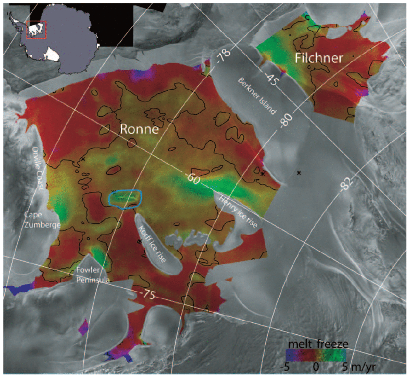
We applied Equation 1 to the FRIS using data from various sources. We have mapped surface velocity with errors in the range of about 2–6ma–1 over nearly the entire FRIS using methods described by Reference JoughinJoughin (2002).We derived an ice-thickness map (see next section) using radar altimeter data (Reference Bamber and BindschadlerBamber and Bindschadler, 1997) and an assumption of hydrostatic equilibrium. The InSAR and altimetry data were acquired over a 2 year period (1995–96). We assume any changes to the ice-shelf speed and thickness over this period are negligible. For surface accumulation, we used an average of two accumulation maps (Reference Vaughan, Bamber, Giovinetto, Russell and RVaughan and others, 1999; Reference Giovinetto and ZwallyGiovinetto and Zwally, 2000). Using Equation 1 applied to these datasets, we computed the basal accumulation map shown in Figure 1, which is a slight update of an earlier version (Reference Joughin and PadmanJoughin and Padman, 2003).
Basal accumulation rates for the FRIS shown in color over a gray-scale synthetic aperture radar (SAR) mosaic (Reference JezekJezek, 1999). The color bar saturates at magnitudes >5ma–1. The zero basal accumulation contour is shown in black. Negative values imply melt, and positive values freezing. The blue outline surrounds an area of probable error identified in the text. The results here have been smoothed to a resolution of about 25 km, but unsmoothed values were used to calculate marine-ice thicknesses.
A positive basal accumulation implies that marine ice is accumulating beneath the ice shelf. Along a flowline, the change in thickness of the marine-ice layer, Hma, is given by

where s is the distance along the flowline (positive along flow). Starting at some initial point where we assume Hma = 0, marine-ice thickness was estimated by integrating Equation 1 along a flowline. Because the marine-ice layer cannot have negative thickness, we solve Equation 1 subject to the constraint that Hma ≥ 0 at all points along the flowline.
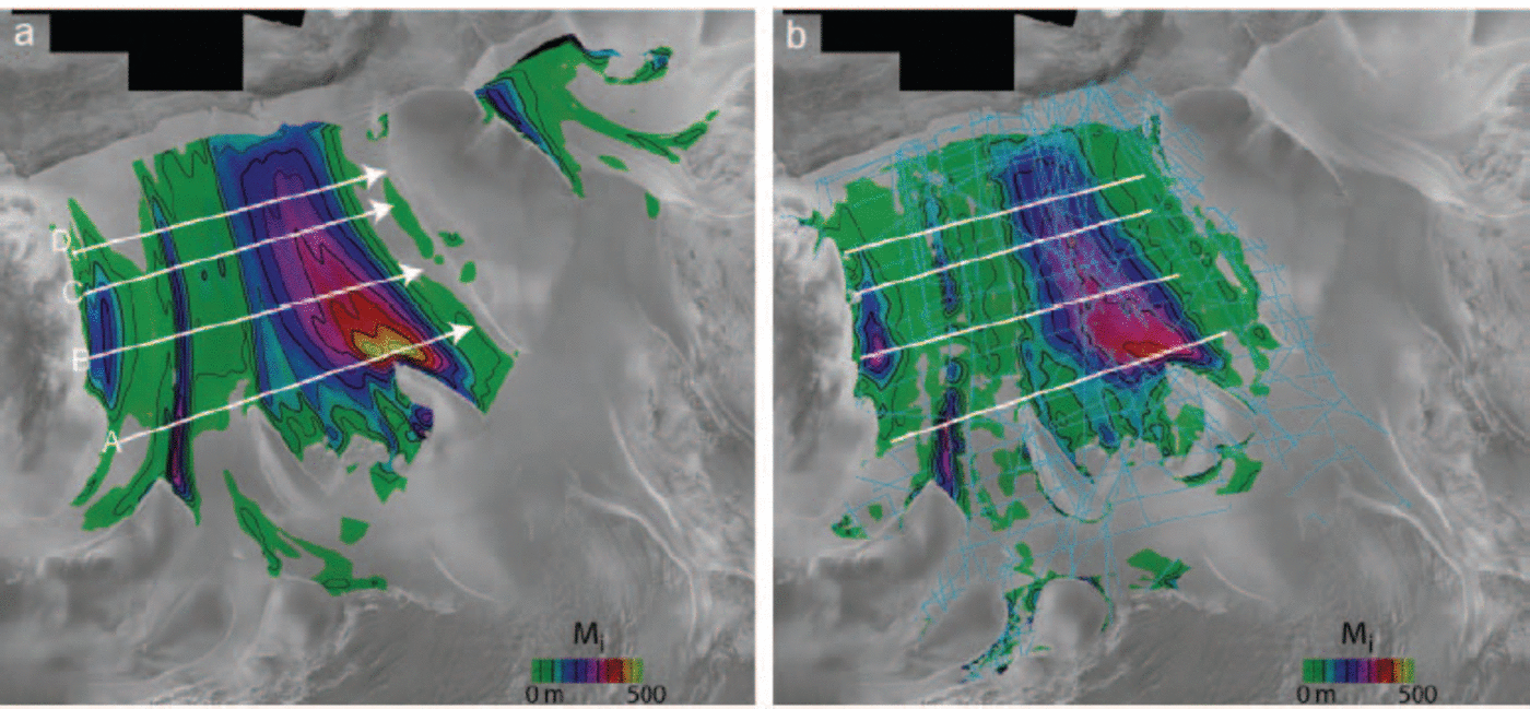
Using the InSAR velocity vectors, we computed flowlines on the ice shelf spaced about 2 km apart. Next, Equation 1 was used to determine marine-ice thickness for each flowline. Since most of the flowlines extended to the grounding line (except where there were data gaps), Hma = 0 was assumed at the upstream end of each flowline. Finally, the flowline results were Delaunay interpolated to a regular grid and then smoothed to a resolution of about 10km to produce the map shown in Figure 2a.
Marine-ice distributions (color and contours) derived using (a) Equation 1 with basal accumulation rates from Figure 1, and (b) difference between RES and hydrostatic thickness. White lines show locations of profiles A–D plotted in Figure 3, with arrowheads indicating direction of increasing distance. Thicknesses are contoured at 50 m (thin) and 100 m (thick) intervals. Light blue lines show the location of the RES data.
RES-based estimate of marine-ice thickness
Marine ice is lossy, and thus rapidly attenuates the pulses used in RES. This means that RES is not generally capable of sounding marine-ice bodies that are more than about 50m thick (Reference JenkinsJenkins and Doake, 1991). Thus, when marine ice is present beneath an ice shelf, the strongest return is almost invariably from the marine-/meteoric-ice interface. RES-derived maps of shelf-ice thickness thus represent meteoric thickness, Hme, rather than absolute thickness, H (Reference Crabtree and C.S.M. DoakeCrabtree and Doake, 1986; Reference ThyssenThyssen, 1988; Reference JenkinsJenkins and Doake, 1991). With accurate elevation data, an assumption of hydrostatic equilibrium can be used to estimate H (Reference ThyssenThyssen, 1988), so that marine-ice thickness can be determined by (Reference JenkinsJenkins and Doake, 1991)

To determine the meteoric-ice distribution, we used RES data collected along the flight-lines shown in Figure 2b. The RES surveys were carried out during a series of campaigns by several institutes using different airborne radar systems. Detailed descriptions of processing and analysis of the individual RES datasets are given by Reference Robin, Doake, Kohnen, Crabtree, Jordan and MöllerRobin and others (1983), Reference Crabtree and C.S.M. DoakeCrabtree and Doake (1986), Reference ThyssenThyssen 1988, Reference Thyssen, Miller and Oerter1991), Reference Vaughan, Doake, Mantripp, Miller and OerterVaughan and others (1991), Reference Thyssen, Bombosch and SandhägerThyssen and others (1993), Reference Hempel, Oerter and OerterHempel and Oerter (1995), Reference Lambrecht, Mayer, Hempel, Nixdorf and OerterLambrecht and others (1997, Reference Lambrecht, Mayer, Oerter and Nixdorf1999) and Reference Grosfeld, Hellmer, Jonas, Sandhäger, Schulte, Vaughan, Jacobs and WeissGrosfeld and others (1998). We combined the different RES datasets of meteoric-ice thickness into a single database and then performed an overall gridding to a polar stereographic grid using a simple Delaunay triangulation algorithm.
When hydrostatic equilibrium is assumed, absolute ice thickness can be determined from (Reference JenkinsJenkins and Doake, 1991)

where h represents elevation above the geoid, e represents errors in the geoidal reference, d is the equivalent thickness of air in the ice column, and ρw and ρi are the densities of water and ice, respectively. Equation 1 provides a linear relationship between elevation and thickness, so it can be re-expressed as

where A and B are the slope and intercept. In several cases, these values have been determined empirically (Reference ThyssenThyssen, 1988; Reference JenkinsJenkins and Doake, 1991; Reference Lythe and VaughanLythe and others, 2001).
The BEDMAP dataset (Reference Lambrecht, Mayer, Oerter and NixdorfLythe and others, 2001) uses a value of B = –148 m, which was applied to all Antarctic ice shelves. This value is significantly larger than values determined for the Ronne Ice Shelf (Reference ThyssenThyssen, 1988; Reference Jenkins and C.S.M. DoakeJenkins and Doake, 1991). Even for the two relations developed specifically for the Ronne Ice Shelf, the relative differences can exceed 20 m. Because of these differences and because we are relying on a different elevation dataset (Reference Bamber and BindschadlerBamber and Bindschadler, 1997) so that the empirical relationships may not hold exactly (i.e. because B subsumes any datum differences), we performed a new fit for the parameters in Equation 1.
We extracted all the seismic and ice-core measurements of H from the BEDMAP online database (Reference Lambrecht, Mayer, Oerter and NixdorfLythe and others, 2001). Next, we culled outliers and points that were close to the grounding line. Since we are primarily interested in the thinner parts of the shelf where marine ice is formed, we also discarded all points with thickness >1000 m. We then extracted the corresponding elevations from the radar-altimeter-based digital elevation map (DEM), which is referenced to the Ohio State University 1991 (OSU91) geoid (Reference Bamber and BindschadlerBamber and Bindschadler, 1997). Using these data we performed a least-squares fit for the parameters in Equation 1, which yielded

If no geoid anomalies are assumed, this result yields a value of d = 11.1m, which is about 3m smaller than earlier values (Reference ThyssenThyssen, 1988; Reference Jenkins and C.S.M. DoakeJenkins and Doake, 1991). This value, however, may compensate for any differences between the true geoid and the OSU91 model and any systematic errors in the DEM.
After computing ice thicknesses using Equation 1, we compared the results against the direct measurements of the thickness from the BEDMAP database. We found a linear trend with distance in the x coordinate (left to right across the images in Figures 1 and 2). This trend may represent spatial variability in the conversion parameters (A, B), a spatially dependent geoid error, or some other systematic error in the elevation dataset. An empirical fit gave a correction of

where x is the coordinate directed along 90˚ E for a polar stereographic coordinate system with a rotation of 0 and standard latitude of 71˚ S. This correction was added to the result from Equation 1 to obtain the final ice-thickness data. Note that because x varies from roughly –1400 km (ΔH ≈ 12 m) to –880km (ΔH ≈ –11 m) across the Ronne Ice Shelf, despite the large intercept, no significant bias is added in the ΔH correction.
Using the meteoric and absolute thickness data, we applied Equation 1 to estimate Hma at points along the flight-lines shown in Figure 2b. Next, we interpolated the points to a regular grid using Delaunay triangulation. Finally, the interpolated result was smoothed to an approximate resolution of 10 km. The resulting RES marine-ice thickness map is shown in Figure 2b.
Comparison of marine-ice thickness estimates
Figure 2 shows three main areas of marine-ice accumulation beneath the Ronne Ice Shelf, which are consistent with the locations shown in earlier maps (Reference ThyssenThyssen, 1988; Reference Bombosch and JenkinsBombosch and Jenkins, 1995). The largest body originates from the area of strong basal freezing adjacent to and downstream of Henry ice rise. Lesser freezing between Henry and Korff ice rises also contributes to this marine-ice mass. A second long, narrow body of marine ice is formed by freezing just downstream of Fowler Peninsula. The third major body of marine ice begins near Cape Zumberge and extends northeastwards along the Orville Coast. We did not have sufficient RES coverage to map marine-ice thickness for the Filchner Ice Shelf, but the InSAR results show a marine-ice body on the west side of the shelf that agrees well with a layer detected by RES and other methods (Reference Grosfeld, Hellmer, Jonas, Sandhäger, Schulte, Vaughan, Jacobs and WeissGrosfeld and others, 1998).
On the Ronne Ice Shelf, there is good overall agreement between the two maps. There are some noticeable interpolation artifacts in the RES map. In particular, there are several gaps in the marine ice originating from the area near Fowler Peninsula that are obviously the result of interpolation errors resulting from the sparse RES coverage.
Figure 3 shows a comparison of the InSAR and RES estimates along the four profiles shown in Figure 2 (white lines). In most cases, the InSAR and RES estimates agree to within the level of uncertainty of the RES measurements. Of the four profiles, the largest differences occur at a position of ~360km along profile A. Examination of the RES coverage shown in Figure 2b indicates there are no direct measurements over most of this region. This was probably because the region is heavily crevassed, creating too much near-surface dispersion of radio energy to give RES basal returns (Reference VaughanVaughan and others, 1994). Such dense crevassing has been associated with the highly extensional flow in areas of high rates of marine-ice accretion (Reference Grosfeld, Hellmer, Jonas, Sandhäger, Schulte, Vaughan, Jacobs and WeissGrosfeld and others, 1998). Thus, the large difference visible in profile A may be the result of errors in the interpolation of the sparse RES data. If this explanation is correct, then in this area the InSAR-derived marine-ice thickness map may be the most reliable, and this map suggests that the marine ice may be nearly 500m thick in this region.
Plots of InSAR and RES estimates of marine ice along profiles A (a), B (b), C (c) and D (d) shown in Figure 2. The dashed line shows results from an alternative estimate that has no freezing in the region around the rift (see text). Error bars indicate the uncertainty (50m) in the RES-derived estimate.

Alternatively, noting that the InSAR estimate is consistently thicker (~50 m) in the corresponding region of the downstream profiles, the large difference in profile A may, at least in part, be the result of an InSAR overestimate in the region of high basal accumulation, which is propagated by the calculation downstream to the other profiles. For the western half of the marine-ice layer originating near Henry ice rise, there is good agreement between RES and InSAR estimates in all four profiles.
The InSAR marine-ice estimates are generally thicker than the RES results in the region from about 150 to 200 km in profiles B–D, which corresponds to the area between the marine-ice layers originating from Henry and Korff ice rises and Fowler Peninsula. For the InSAR estimate, most of the marine ice in the region is formed in the area of strong basal accumulation centered on a large rift just downstream of Korff Ice Rise (see blue outline in Fig. 1). The rift likely introduces an error in the hydrostatic thickness solution that then leads to erroneously large freezing rates. To evaluate the effect of this error, we created an alternate thickness map by setting the basal accumulation rate to zero in the region outlined in blue in Figure 1, which decreases basal accumulation by 2.5 Gtons a–1. The result is shown by a dashed line in Figure 3 and, in most cases, it agrees to within the RES error bars.
The RES and InSAR estimates show generally good agreement for the Fowler Peninsula marine-ice layer, with a significant difference visible only for profile B. Inspection of Figure 2b indicates that this difference is a result of the type of interpolation errors described above. There is also reasonable agreement between the profiles for the marine ice along the Orville Coast. The moderate differences in the shapes of the profiles are also probably the result of interpolation errors in regions with sparse RES coverage.
To avoid the influence of interpolation errors, we also compared the InSAR estimates of marine-ice thickness directly with the RES data at the points shown in Figure 3. The average marine-ice thickness from the InSAR data was 132 m compared to 119m for the RES estimate, giving a mean difference of 13 m. The overall root-mean-squared difference (rms) was 46m. We performed a similar comparison with the alternate InSAR estimate that had the basal accumulation rates zeroed near the rift. In this case, the mean thickness was reduced to 129 m, giving a mean difference of 10 m. Equation 1 indicates the hydrostatic solution for thickness could introduce a bias into the RES data of ±4.8m. Given the range of estimates based on similar data (Reference ThyssenThyssen, 1988; Reference Jenkins and C.S.M. DoakeJenkins and Doake, 1991), we believe the uncertainty in the mean RES thickness could be ±10m or larger. In addition, there is an unknown level of
uncertainty in the InSAR estimates of at least several meters. Thus, the RES and InSAR estimates both predict mean marine-ice thicknesses that are consistent to within the anticipated levels of uncertainty.
Discussion
As noted above, without accurate characterization of the errors in the total ice thickness inferred from the hydrostatic inversion of altimeter data, it is difficult to estimate the uncertainty in the basal accumulation rates, and this is largely the reason for completing the present comparison. The two most likely sources of error are errors in the velocity and thickness gradients in Equation 1. Thus, it is informative to examine how these types of error impact basal accumulation estimates. The first bracketed term in Equation 1 includes the ice-thickness gradient. Since an ice shelf generally thins parallel to flow, a highly oversimplified model for an ice shelf is a wedge of ice moving at constant velocity. In this case, the first term in Equation 1 indicates that melt is required to maintain a steady-state profile. The second bracketed term in Equation 1 contains the velocity gradients. This leads to a second simplified model where an ice shelf is considered to be a slab of uniform thickness that spreads and thins. In the absence of surface accumulation, this model requires basal freeze-on to maintain a constant thickness.
Although the models just described are oversimplified, they indicate how, for a steady state, ice-shelf dynamics relate to and are balanced by the total accumulation rate ( ȧb + ȧs). First, basal and surface melt are generally accommodated by the ice-shelf geometry, which typically thins along flow. Second, basal and surface accumulation are largely balanced by ice-shelf flow, which is mostly extensional (Reference Grosfeld, Hellmer, Jonas, Sandhäger, Schulte, Vaughan, Jacobs and WeissGrosfeld and others, 1998). The balance of these two terms determines whether there is net accumulation or ablation at any given location. These points are illustrated by the results shown in Figure 4, which shows the values for the two bracketed terms in Equation 1 that went into the calculation of the basal accumulation rates (Fig. 1).
Results for bracketed terms (a)  in Equation 1 that went into the basal accumulation estimate given in Figure 1. Results have been smoothed to ~25km resolution, and the zero contour is shown in black.

Figure 4a reveals that the along-flow thinning gradient of the ice-shelf profile yields a melt-like contribution over most of the shelf. This term is particularly strong at the grounding lines and the ice front, where the thickness gradients are largest. This term is much smaller (near zero) close to the center of the shelf where the thickness is nearly uniform. Figure 4b shows that the areas of strong freezing (up to 5 ma–1) are located where there are strong velocity gradients from stagnant grounded areas (e.g. Henry ice rise) to the fast-moving shelf. In the central part of the shelf where the melt term is small, the extensional flow yields a large area of moderate (20–80 cm a–1) basal freezing (see Fig. 1).
The good agreement between the RES and InSAR marine-ice estimates helps validate the basal accumulation rates from the high-growth regions and central shelf all the way to the ice front, where high melt rates remove the accumulated marine ice. This is because in the high-growth regions, as Figure 4b illustrates, the ‘freezing’ related to extension is much larger than the corresponding ‘melt’ related to thickness gradients. As a result, the high basal accumulation rates largely reflect gradients in the relatively reliable velocity data as opposed to the less reliable thickness gradients. Toward the nearly flat center of the shelf where the ‘melting’ and ‘freezing’ in Figure 4 are comparable in magnitude, reasonable results likely are obtained because the thickness data should be more reliable in this region.
The ability of the InSAR basal accumulation rates to reproduce the marine-ice thickness distribution does not validate the large basal melt rates near the ice-stream grounding lines. This is because the marine-ice estimates only include basal accumulation rates downstream of the location where marine ice is first formed. Figure 4 reveals that the melt estimated at the grounding line is largely determined by thickness gradients, although compressive flow sometimes contributes to a lesser extent. This is precisely the region, however, where hydrostatic thickness estimates are likely to be biased toward thicker values by topography-induced altimeter errors near the grounding lines. Thus, thickness errors may cause overestimation of grounding-line melt. Such biases are probably not too large, particularly when averaged, since shelf-wide averages of basal accumulation determined using Equation 1 agree well with values determined from flux gates around the ice-shelf perimeter, which make greater use of unbiased RES thickness estimates (Reference Joughin and PadmanJoughin and Padman, 2003). Validation of continuity-based melt estimates near grounding lines will likely require independent estimates such as those available from phase-sensitive radar (Reference Hempel, Oerter and OerterCorr and others, 2002).
Another reason for the good agreement between the RES and InSAR estimates is that basal accumulation errors tend to cancel when integrated along flowlines or averaged over wide areas. Averaging is particularly effective because thickness anomalies generally introduce matched positive and negative thickness gradient anomalies, yielding areas of erroneous melting and freezing that more or less cancel when averaged. An example of this phenomenon can be seen about midway between the rift and the shelf front in Figure 1, where an upstream area of enhanced melt is balanced by a downstream region of enhanced freezing.
We note that the two marine-ice thickness distributions (Fig. 2) are not truly independent in that they both rely on the same altimeter-derived thickness data, H. Nevertheless, the ways in which errors in H impact each estimate are different. For the RES-based estimate, an error in H directly yields a local error Hma. In contrast, the same thickness error introduces a local error in the basal accumulation rate, which is propagated through Equation 1 into a distributed error in the estimated Hma. Thus, although they rely on a common dataset, the two marine-ice distributions, for the most part, can be considered independent.
The problems of hydrostatically determined thicknesses using altimeter data should be largely overcome with the next generation of space-borne altimeters such as the Geoscience Laser Altimeter System (GLAS) and CryoSat. With these data, hydrostatic thicknesses should have significantly reduced altimeter-induced biases, except in narrow embayments or very close to the grounding line, where there could be significant departures from hydrostatic equilibrium.
Summary
The basal accumulation rates shown in Figure 1 yield average marine-ice thicknesses that agree with the RES observations to within a difference of about 10%. This result suggests that the basal accumulation rates derived from InSAR velocity and altimeter-derived thicknesses, particularly when averaged over wide areas, provide a reasonable estimate of basal accumulation. Such a conclusion cannot yet be reached for areas near the grounding lines, where further validation is needed. If we consider the mean RES marine-ice thickness to be reliable to within about ±10%, then the 10% difference between estimates suggests that the InSAR estimates are correct to about ±20%. This allows us to roughly quantify the uncertainty in the earlier estimates of 55.6Gtons a–1 of total freezing near the center of the Ronne Ice Shelf and 54.8 Gtons a–1 of melt near the front of the shelf (Reference Joughin and PadmanJoughin and Padman, 2003).
The fact that the basal accumulation rates derived under the assumption of a steady-state ice shelf provide a reasonably accurate estimate of the marine-ice distribution suggests that the center and front of the ice shelf do not depart significantly from steady-state conditions over the long term. Any recent departure (e.g. within the last several decades) from steady state would likely not yet have yielded changes in marine-ice volume that are sufficiently large to be detected by our comparison.
Acknowledgements
I.J. performed this work at the Jet Propulsion Laboratory, California Institute of Technology, under contract with the National Aeronautics and Space Administration. We thank H. Sandhäger and all those at the British Antarctic Survey, the Alfred Wegener Institute and Westfalische Wilhelms-Universitat, Münster, Germany, who were involved in collecting the RES data. In addition, we thank J. Bamber (ice-shelf DEM), M. Giovinetto (surface accumulation), K. Jezek (SAR mosaic), L. Padman (tide model) and the staff at the Alaska SAR facility (raw SAR data). Reviews by S. Jacobs and A. Shepherd and editorial comments by H. Fricker led to significant improvements in the final manuscript.



