Introduction
The meaning of the term home range emerged in an exclusively spatial context whereby the animals restrict their most routine movements to a specific area (Darwin, Reference Darwin1861; Seton, Reference Seton1909). Later, Burt (Reference Burt1943) described it as ‘the area traversed by an individual in its normal activities of food gathering, mating, and caring for young. Occasional sallies outside the area, perhaps exploratory in nature, should not be considered part of the home range’. In other words, non-nomadic animals that live in a defined area where they enact their day-to-day activities (Powell, Reference Powell, Pearl, Boitani and Fuller2000). The definition of Burt (Reference Burt1943) assumes that every location within a home range is of equal importance to the individual (Don, Reference Don1949; Seaman & Powell, Reference Seaman and Powell1996; Sprogis et al., Reference Sprogis, Raudino, Rankin, MacLeod and Bejder2016). Other definitions include a time factor i.e. the area where the animals spend 95% of the time for daily activities is considered the home range, whilst the areas in which they spend at least 50% of the time is considered the core area (Dixon & Chapman, Reference Dixon and Chapman1980; Samuel et al., Reference Samuel, Pierce and Garton1985; White & Garrott, Reference White, Garrott, White and Garrott1990); however, Bertrand et al. (Reference Bertrand, DeNicola, Beissinger and Swihart1996) recommend studying two levels of core area, 45% and 25%. Cognitive factors can also be included; the knowledge of animals about the area they inhabit may be considered in any definition of home range (Peters, Reference Peters, Hall and Sharp1978; Powell, Reference Powell, Pearl, Boitani and Fuller2000; Börger et al., Reference Börger, Franconi, Ferretti, Meschi, DeMichele, Gantz and Coulson2006; Spencer, Reference Spencer2012), with information about important routes and resource location (Powell, Reference Powell, Pearl, Boitani and Fuller2000; Kie et al., Reference Kie, Matthiopoulos, Fieberg, Powell, Cagnacci, Mitchell, Gaillard and Moorcroft2010). Finally, Powell & Mitchell (Reference Powell and Mitchell2012) proposed ‘the best concept of a home range is that part of an animal's cognitive map of its environment that it chooses to keep updated’.
Nekolny et al. (Reference Nekolny, Denny, Biedenbach, Howells, Wendy, Mazzoil, Durden, Moreland, Lambert and Gibson2017) consider that extrinsic and intrinsic factors influence the home range, primarily the quality and richness of prey, the predation risk and anthropogenic activity. Secondary factors are physiological limitations, reproductive status, hetero-specific behaviours and individual body size. It is also necessary to consider that the home range size can be sex-specific and that the differences in size and location could have implications for conservation (Wearmouth & Sims, Reference Wearmouth and Sims2008).
The size of the geographic range of populations is often underestimated in home range studies. This occurs due to factors such as funding and research constraints limiting the area studied. This is usually appreciated when the cumulative curve of area by sightings does not reach the asymptote (Ingram & Rogan, Reference Ingram and Rogan2002) but also when individuals are detected outside the study area and estimated home range (Gruber, Reference Gruber1981; Fury & Harrison, Reference Fury and Harrison2008). This potential issue is accentuated in higher latitudes where populations have a greater tendency to migrate. It is therefore important to take these factors into account to ensure a precise estimate of the home range.
Tursiops truncatus is a predator with efficient swimming capacity; it is expected to have an extensive home range (Ingram & Rogan, Reference Ingram and Rogan2002). However, it is also known that the size of the home range of T. truncatus has frequently been limited by physiographic changes that increase the water depth such as channels or submarine canyons (Wells & Scott, Reference Wells, Scott, Perrin, Wursig and Thewissen2002). The first estimate of home range for this species was recorded by Caldwell (Reference Caldwell1955) based on a single individual in the Atlantic ocean ‘with dorsal damage’ on the coast of Georgia and South Carolina (USA). The estimated range was 175 km along the coastline and it was apparent that this individual could have been travelling from one area to another and, therefore, this individual and conspecifics could have seasonal home ranges. More recently, Nekolny et al. (Reference Nekolny, Denny, Biedenbach, Howells, Wendy, Mazzoil, Durden, Moreland, Lambert and Gibson2017) collected data and estimated the home range of T. truncatus, from 20–343.89 km2 and represented a percentage of coverage of 1.08–104% from the study area.
The home range is a measure of biological interest. Gubbins (Reference Gubbins2002) remarks that apart from the need to understand animal movement, aspects such as social organization, mating behaviour and the dynamics of disease transmission are also implicit. The home range is also of conservation interest when considering threatened populations (Seminoff et al., Reference Seminoff, Resendiz and Nichols2002; Maxwell et al., Reference Maxwell, Breed, Nickel, Makanga-Bahouna, Pemo-Makaya, Parnell, Formia, Gouessono, Brendan, Costa, Witt and Coyne2011) or those that regularly interact with humans (Rayment et al., Reference Rayment, Dawson, Slooten, Bräger, Fresne and Webster2009). However, this scenario could be more complex when home ranges of one species overlap with the home range of another – both marine and human. Localities with such overlap have ecological and conservation importance (1) because those spaces could potentially offer a constant source of food and shelter, and (2) because they should be identified for protection since habitat conservation contributes to the conservation of more than one species.
The western coast of Aragua State, Venezuela, is an oceanic coast with semi-enclosed (bays and sounds), open and neritic habitats that hosts a resident population of bottlenose dolphins but is also frequented by non-resident dolphins throughout the year. This coastal region is also inhabited by a population of Atlantic spotted dolphin Stenella frontalis that occurs all year round and is sighted more frequently than T. truncatus (Cobarrubia-Russo, Reference Cobarrubia-Russo2010; Cobarrubia-Russo et al., Reference Cobarrubia-Russo, Barreto, Quintero-Torres, Molero-Lizarraga and Xianyan2018). The purpose of this study is to estimate the home range of resident Tursiops truncatus individuals and analyse the ranges of S. frontalis and fishermen in order to detect possible overlaps that could define an area of extreme importance to be considered for greater conservation protection.
Materials and methods
Study area
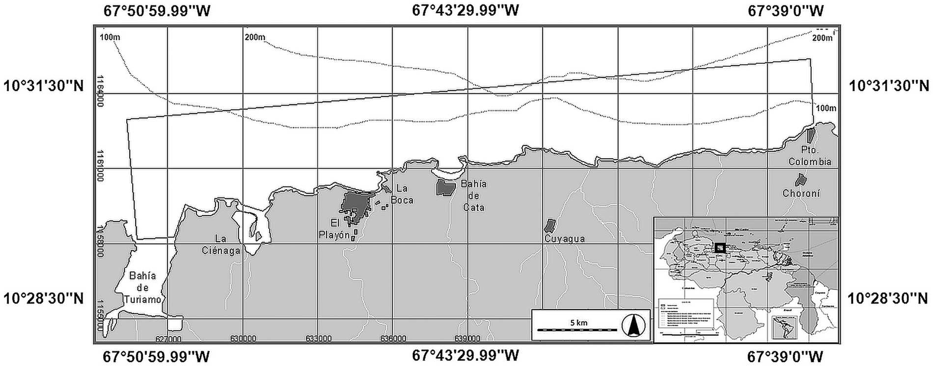
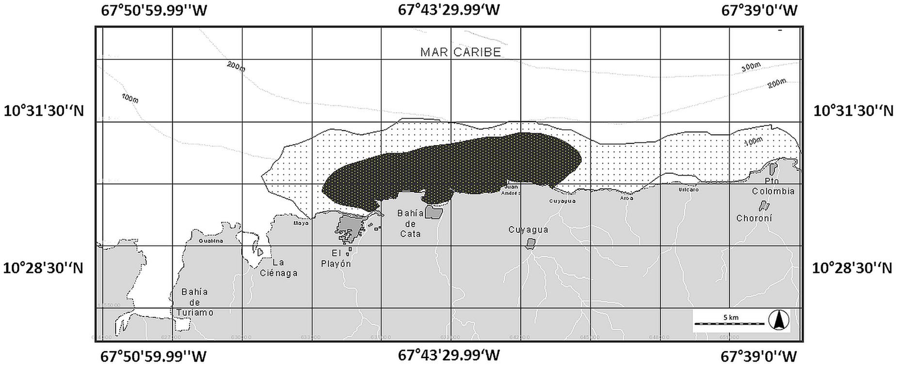
The study area is a coastal strip of ~30 km long and ~3 km wide, from Turiamo Bay (10°28′N 67°50′W) to Puerto Colombia (10°30′N 67°36′W) encompassing ~92.12 km2 (Figure 1). According to Novoa et al. (Reference Novoa, Mendoza, Marcano and Cárdenas1998), sea surface temperature is 25–27°C, with salinity ranges of 34–36 ppm, a tidal regime of ±24 cm and two seasons (Dry: November–April. Rainy: May–October). Also present is an unusual upwelling of matter from Codera Cape including chlorophyll and dissolved organic matter (Bolaños-Jiménez et al., Reference Bolaños-Jiménez, Castro-Pérez, Herrera-Trujillo, Oviedo, Palacios, Sánchez-Criollo, Puerto, Sifontes, Silva-Hernández and Villarroel-Marín2013). The study area consists of rocky cliffs, some sandy beaches and hosts three marine habitats, according to Gowans et al. (Reference Gowans, Würsig and Karczmarski2008). The first habitat involves semi-enclosed bays such as (from left to right) Turiamo Bay, La Ciénaga Sound, El Playón-La Boca Bay and Cata Bay (Figure 1). The second habitat is from the coastline to the 100 m isobath, from near Cuyagua beach to the outside of Turiamo Bay, progressively moving away from the coastline as it moves westward (Figure 1). The third habitat occupies an area that is limited to the south by the coastal axis and to the north by the 200 m isobath, and is predominately located towards the western end of the study area (Figure 1).
Study area.

Field surveys, sightings and photo-ID
Field surveys were carried out between May 2004 and October 2008, on a predefined transect of 30 km, ~1.5 km parallel to the coast. Each started at the western end (Turiamo Bay) of the study area and ended to the eastern end (Puerto Colombia) (Figure 1). The mean speed of the vessel was ~7 knots in a 9 m long 45 HP outboard-powered boat with three observers on board (one on the bow, one on the port and one on the starboard).
When a dolphin or dolphin pod was encountered, we deviated from the transect and approached slowly to a distance of ~10 m and recorded the following information: observation time, pod size and location (using a hand-held Global Positioning System). A pod of dolphins was defined as all dolphins within a 100 m radius of each other and engaged in similar activities (Irvine et al., Reference Irvine, Scott, Wells and Kaufman1981). Latitude and longitude of fishing boats and other cetacean species were also recorded. In the study area S. frontalis appears more frequently than T. truncatus and is also present throughout the year (Acevedo, Reference Acevedo2007; Cobarrubia-Russo, Reference Cobarrubia-Russo2010; Cobarrubia-Russo et al., Reference Cobarrubia-Russo, Barreto, Quintero-Torres, Molero-Lizarraga and Xianyan2018).
After the initial encounter with T. truncatus, an observer photographed every individual possible for photo-identification. Photographs of individuals were taken using a Canon Rebel XTI DSLR camera body fitted with an autofocus Canon 18–200 or Tamron 18–250 mm zoom lens using Large/Fine resolution and RAW format. Individual dolphins were identified by natural marks (permanent marks suitable for reliable long-term identification) on the body and the trailing edge of their dorsal fins (Würsig & Würsig, Reference Würsig and Würsig1977; Wilson et al., Reference Wilson, Thompson and Hammond1997). The photo-identification effort time depended on the size of the pod and behaviour towards the vessel; at the end of each photo-identification session, the boat returned to the transect to complete it in search for other pods.
Only high-quality photographs with clear identification of marked individuals were used for analysis (i.e. those in focus, with the dorsal fin perpendicular to the plane of the photograph or close enough to identify small notches) (Díaz López & Bernal-Shirai, Reference Díaz-López and Bernal-Shirai2007, Reference Díaz-López and Bernal-Shirai2008). A marked individual was defined as an individual recognized by more than one feature. Repeated sightings of individuals on the same day were treated as a single sighting. The photographs were independently reviewed and selected by the three observers and each then analysed utilizing the Finscan 1.6.1 program in order to minimize identification errors (Hillman et al., Reference Hillman, Kehtarnavaz, Wursig, Araabi, Gailey, Weller, Mandava and Tagare2002). Once identification was confirmed, the individual was assigned an alpha-numeric ID code (D ##). Finally, each identified pod was assigned a letter from A to Z according to the chronological order of their identification, i.e. the first dolphin 1 (D01) from the first pod (A) would be coded as AD01.
Identification of individual home ranges of Tursiops truncatus
Only the records of adult individuals were chosen for home range analysis. Juveniles and calves were excluded because they lack sufficient marks. Rapid ontogenetic changes are also a known source of bias in photo-identification (Welsh et al., Reference Welsh, Goatley and Bellwood2013). The estimates of home range depended on the number of sightings of each individual (Cameron & Spencer, Reference Cameron and Spencer1985), tending to increase the area with each new sighting until reaching a maximum (Mares et al., Reference Mares, Willig and Bitar1980; Anderson, Reference Anderson1982). For T. truncatus, a minimum of 20 sightings was required for inclusion, as has been recommended in previous studies (Mares et al., Reference Mares, Willig and Bitar1980; Schoener, Reference Schoener1981; Gubbins, Reference Gubbins2002). The Transverse Universal Mercator Coordinate System (UTM, Zone 19P North) was used, based on the 1984 WGS datum. We determined the accumulated polygonal area for each new sighting. In the case of individuals whose saturation curve reached an asymptote, we proceeded to use GIS (Arcview 3.3 ESRI) to estimate home ranges by the most used and comparable approaches, Minimum Convex Polygon (MCP) (Mohr, Reference Mohr1947) and Fixed Kernel (FK) (Van Winkle, Reference Van Winkle1975; Worton, Reference Worton1987; White & Garrott, Reference White, Garrott, White and Garrott1990). MCP is the most widely used and simplest method to measure home range size. It is optimized for home ranges of territorial animals and allows delineation between the range and home range by connecting peripheral points constructing a convex polygon (Jenrich & Turner, Reference Jenrich and Turner1969; White & Garrott, Reference White, Garrott, White and Garrott1990; Flores & Bazzalo, Reference Flores and Bazzalo2004). FK is an assessment of probability that determines the frequency of use distribution, allowing a good approximation of the intensity of use by the individual analysed (Silverman, Reference Silverman1986; Gubbins, Reference Gubbins2002). This method was applied using the tool Animal Movement of Spatial Analyst (Arcview 3.3 ESRI). For the calculation of the estimated areas with FK, a smoothing parameter must be chosen – assuming that the data are distributed normally and provide a measure of accuracy of fit based on a cross-validation score of least squares (Worton, Reference Worton1989). Following Burt's (Reference Burt1943) definition of household range and his suggestion that occasional movements outside the area not be included in an animal's home range, we used 95% FK as a measure of home range size, as also recommended by Bertrand et al. (Reference Bertrand, DeNicola, Beissinger and Swihart1996), i.e. there is a 95% probability that the dolphin will be located within the stated area. This was defined as the home range (Worton, Reference Worton1995). We calculated core areas at two levels, 45% and 25%, in order to detect the possibility of individual core areas overlapping. Finally, landmasses, as a natural barrier, were removed from the home range area.
Range of Stenella frontalis
The latitude and longitude records of Stenella frontalis were imported into ArcView 3.3 and ranges estimated using the same methodology as T. truncatus in order to identify areas of possible overlap (Mohr, Reference Mohr1947; Van Winkle, Reference Van Winkle1975; Worton, Reference Worton1987; White & Garrott, Reference White, Garrott, White and Garrott1990).
Fisheries area
The latitude and longitude records of fishing boats were imported into ArcView 3.3. Most of these boats come from five fishing villages in the study area: Ocumare, El Playón, Cata, Cuyagua and Puerto Colombia (the most distant within the study area); however, vessels from other fishing ports also enter the study area. Ranges were estimated using the same methodology as for T. truncatus.
Overlapping zones of usage
The separate FK (45%, core area) ranges identified using ArcView 3.3 for each species (Tursiops truncatus and Stenella frontalis and fishing boats) were superimposed in order to calculate the overlap area.
Results
Sightings
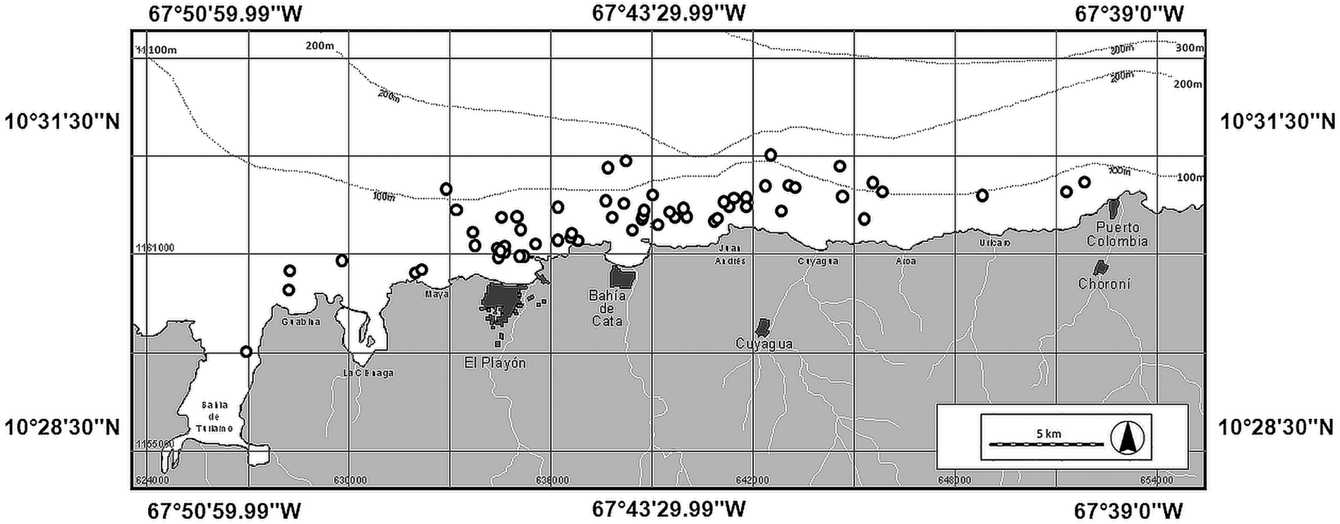
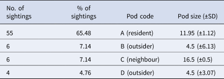
One hundred field surveys were conducted between May 2004 and October 2008. Eighty-four sightings of T. truncatus were recorded in 56 surveys (Figure 2), these sightings enabled the identification of four distinct pods (Table 1).
Sighting records of Tursiops truncatus.

Number of sightings, percentage of sightings, pod code and pod size of Tursiops truncatus

The remaining sightings comprised mixed pods: one of A + B + S. frontalis, five of A + C and two of A + C + S. frontalis.
Ninety-five sightings of Stenella frontalis were recorded. Forty of these were mixed pod sightings with T. truncatus and one sighting with Balaenoptera sp. This other delphinid was not subject of photo-identification. Other species sighted were Delphinus sp. (four records), Stenella longirostris (one record) and a non-identified Ziphidae (one record).
A total of 3360 photographs of T. truncatus were analysed from which 660 (19.64%) were considered to be appropriate for creating a photo-identification catalogue comprising 84 individuals. Of these, only seven (8.33%) were photographed on distinct occasions and thus were selected for individual home range analyses (Figure 3).
Photo-identified individuals whose home ranges were estimated.

Individual home ranges of Tursiops truncatus
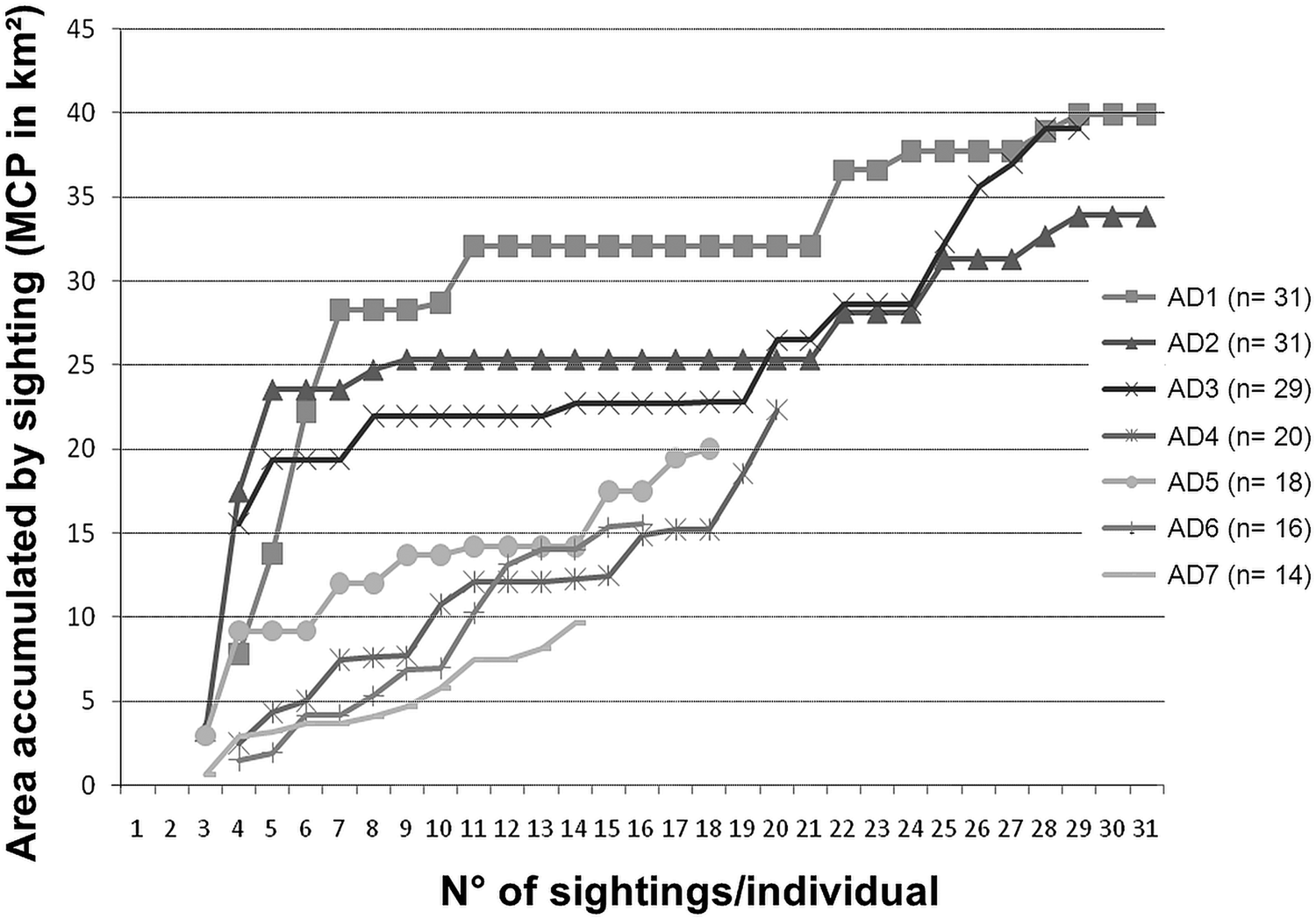
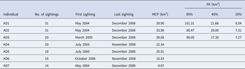
Sightings of Tursiops truncatus covered an area of 56.63 km2 with MCP (Figure 2). The area saturation curves of the seven individuals (AD1–AD7) were plotted (Figure 4). The females AD1, AD2 and AD3 reached a stable asymptote with sightings 19 and 20 (August 2008) although their areas increased later (to 12.5%, 28.6% and 55.3%, respectively). Therefore, only three home ranges by FK were calculated: for AD1, AD2 and AD3; and seven (AD1-7) by MCP, even though AD4-AD7 reported ≤20 sightings in order to reinforce the integrity of the data (Table 2).
Accumulated area of individuals AD1–AD7 (MCP in km2) vs the number of sightings/individual.

Photo-identified individuals, number of sightings, first sighting, last sighting, home range (km2) using Minimum Convex Polygon (MCP) and Fixed Kernel (FK at 95%, 45% and 25%)

For the three dolphins that reached the asymptote of the area accumulation curve, home range was estimated at 33.90–39.90 km2 (MCP; 36.79–43.31% of the study area), and 80.47 and 101.31 km2 (FK) (Table 1). Therefore, individuals AD1 and AD3 exceeded the study area by 109.97% and 104.26%, respectively. The estimation of the core areas at 45% ranged between 17.30–21.66 km2 and at 25% ranged between 7.27–8.54 km2 (Table 1).
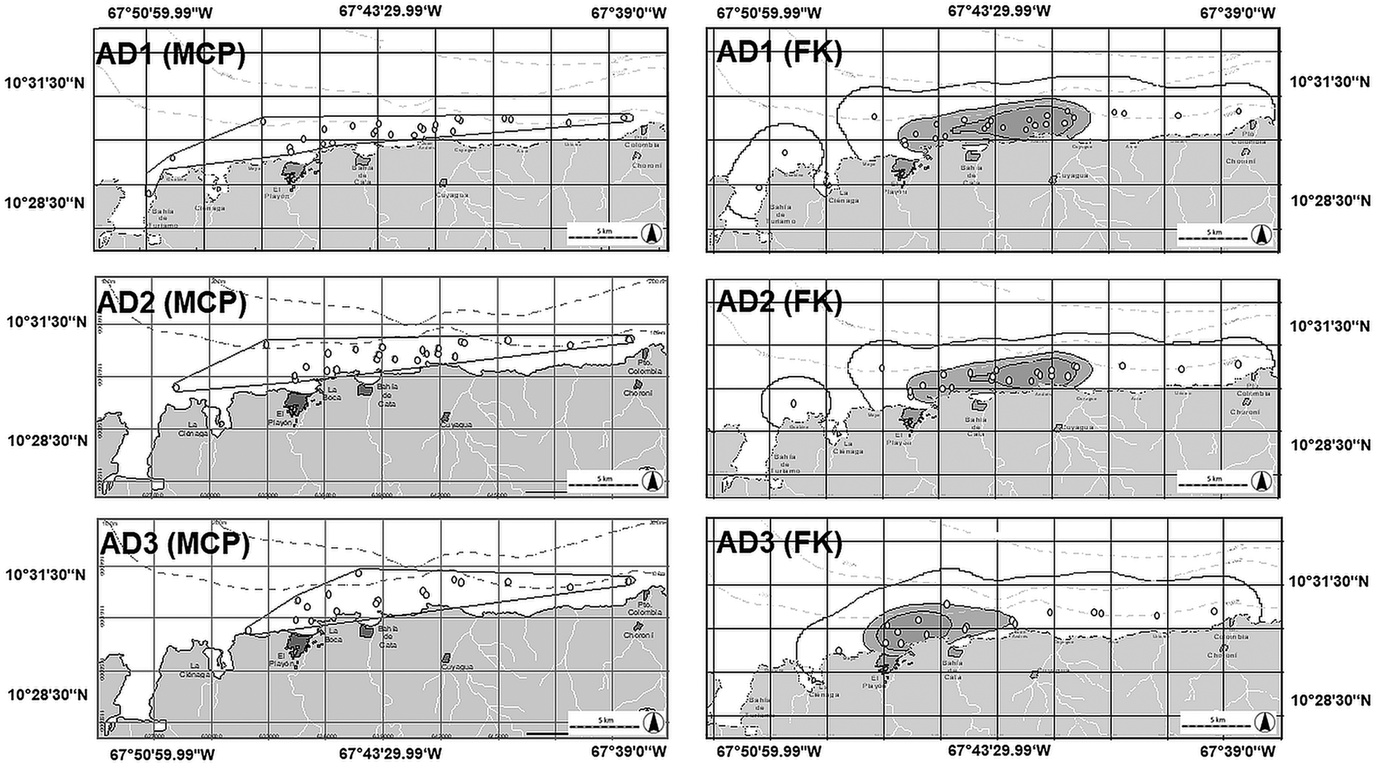
Regardless of the method being used, all individuals (AD1–AD7) showed an overlap of their home range (Figures 5 & 6). Nevertheless, the individual AD3 showed a core area located further west than the other two individuals with no overlap at all with them when analysed at 25% by FK (difference from just 1.66 km2 at 45% and 1.23 km2 at 25%) (Figure 5, Table 1).
Home range of individuals AD1, AD2 and AD3 (above, middle and low) by MCP (left) and FK (right) to 95%, 45% and 25C (white, light gray and dark grey, respectively).

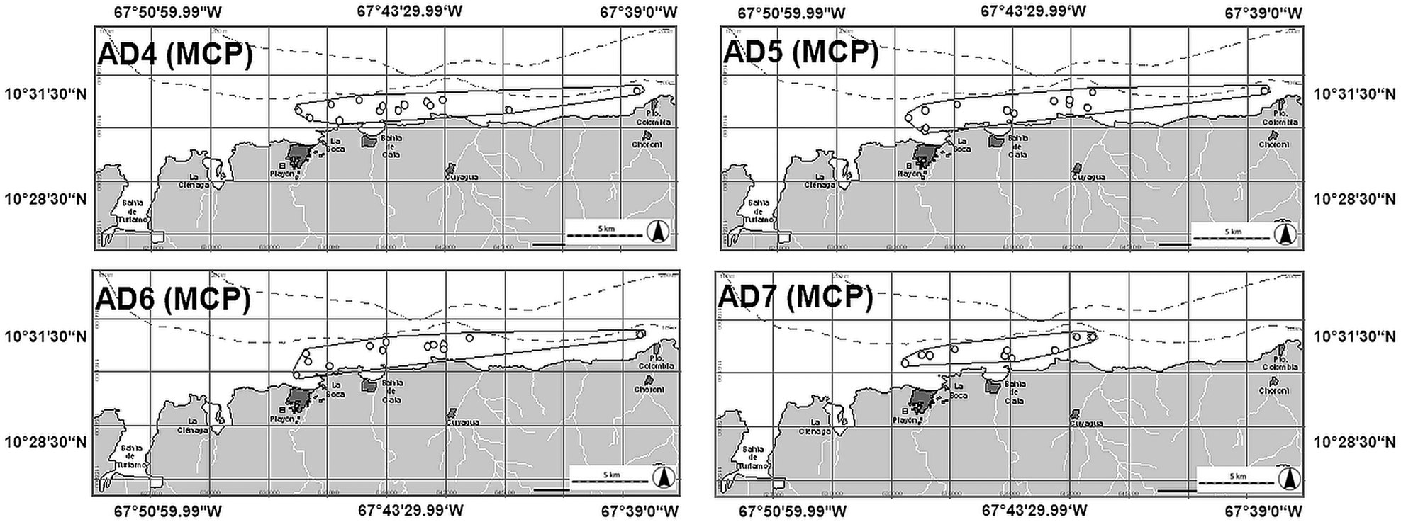
Home range of individuals AD4, AD5, AD6 and AD7 by MCP.

Despite ~20 sightings of AD4–AD7, their area accumulation curves by sighting did not reached the asymptote. It was therefore decided to calculate their MCP to complement the information on pod A. Predominantly sightings were located in the core areas of individuals AD1, AD2 and AD3 (Figure 6).
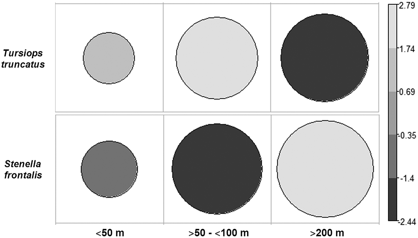
The majority of sightings were located in areas with depths ranging from 51–100 m (54% sightings) (χ2 = 24.5, df = 2, P = 4.785 × 10−06) (Figure 7), with the exception of AD3 that was sighted in a locality with a depth ~140 m. According to the FK analysis, the highest density of sightings was recorded in areas where the depth did not exceed the 100 m isobath, although it should be noted that the three central areas at 45% slightly exceeded the 100 m isobath. At 25% this isobath was excluded (Figure 5). These findings are supported by the recording of individuals AD4–AD7 in localities with depths less than 100 m (Figure 6).
Correlation plot of standardized residuals between sightings of Tursiops truncatus and Stenella frontalis vs depths.

Range of Stenella frontalis
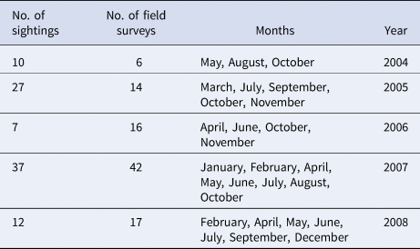
During the study, 95 sightings of S. frontalis were recorded (Table 3), the range extended to 75.23 km2 with MCP (81.66% of coverage on the study area) and 119.86 km2 with FK at 95% (130.11%). The core areas were 19.25 km2 (45%) and 6.77 km2 (25%), showing a complete overlap with pod A of T. truncatus (Figure 8).
Range of Stenella frontalis by MCP (left) and FK (right) to 95%, 45% and 25% (white, light grey and dark grey, respectively).

Number of sightings of Stenella frontalis, number of field surveys, months with sightings records and years

Stenella frontalis was sighted in waters ranging from the internal coast at Turiamo Bay to neritic habitat; 68.29% of sightings were recorded in localities with depths of 101–200 m (χ2 = 24.5, df = 2, P = 4.785 × 10⁻⁶) (Figure 7).
Range of fishermen
During the study, 190 sightings of boats actively fishing were recorded. The calculated range was 93.26 km2 (101.23% of coverage on the study area) with MCP and 228.49 km2 with FK (95%) (245% of coverage on the study area) (Figure 9).
Range of fishermen by MCP (left) and by FK (right) at 95%.

Overlapping zone
The overlapping areas of ranges of pods of Tursiops truncatus, pods of Stenella frontalis and fishermen was 63.31 km2 (FK 95%) and 24.75 km2 (FK 25%), which equated to 26.86% of the study area (Figure 10).
Overlapping of higher density areas (FK) of T. truncatus, S. frontalis and fishermen at 95% (white with black dots) and 25% (black with white dots).

Discussion
This is the first project estimating individual bottlenose dolphin home ranges in Venezuela utilizing photo-identification. We recorded estimates between ~30–40 km2 (with MCP) with their respective area accumulation curve asymptote, while those with ≤20 sightings produced areas between 20–25 km2. This reinforces the argument that more than 20 sightings are necessary to estimate home ranges of T. truncatus (Mares et al., Reference Mares, Willig and Bitar1980; Schoener, Reference Schoener1981; Gubbins, Reference Gubbins2002). It should be noted that the differences in estimated areas are not statistically robust due to the limited number of individuals studied. Other individuals were present but it was not possible to include them in this study as their behaviour was more elusive, resulting in reduced success with photographic recording. The study area has a Beaufort of ~3 throughout the year so this was not significant in hindering recording. During the field surveys, it was noted that whilst the pod A was approachable, it was typically only adult individuals that approached the boat, for example AD1, AD2 and AD3; others were initially more elusive but, over time, became ‘familiar’ with the boat. This is evident in Figure 4 where AD1, AD2 and AD3 accumulated areas between ~ 20–30 km2 from the sightings 5 and 7 while individuals AD4, AD5, AD6 and AD7 never reached the asymptote. A good example of this is that AD4 with 20 sightings barely accumulated 22.5 km2; this supports the theory that behaviour with regards to the presence of a boat influences the estimate of the home range (Nekolny et al., Reference Nekolny, Denny, Biedenbach, Howells, Wendy, Mazzoil, Durden, Moreland, Lambert and Gibson2017).
The photo-identified individuals belonged to a resident pod (A) which was sighted throughout the study. This pod was composed of females, mother-calves and visitors (Cobarrubia-Russo et al., Reference Cobarrubia-Russo, Barreto, Quintero-Torres, Molero-Lizarraga and Xianyan2018). All the individuals for whom the home ranges were estimated by MCP and FK were adult females. In a preliminary study of social structure, these three females proved to have the highest hierarchy and association index and, within the trio, A1 and A2 were the principal matriarchs of the pod with the highest index of association (Cobarrubia-Russo, Reference Cobarrubia-Russo2010).
Therefore, the home ranges of A1 and A2 could be used to estimate the feeding home range of this pod, which demonstrated high site fidelity during the study, due to the fact that most sightings of A1 and A2 include other females and mother-calf pairs (Cobarrubia-Russo, Reference Cobarrubia-Russo2010; Cobarrubia-Russo et al., Reference Cobarrubia-Russo, Barreto, Quintero-Torres, Molero-Lizarraga and Xianyan2018).
Home ranges estimated for this population are small when compared with those previously studied in Texas and Sarasota, USA (Gruber, Reference Gruber1981; Irvine et al., Reference Irvine, Scott, Wells and Kaufman1981). However, it is noted that on the coast of Aragua there is a small area with a plentiful year-round source of prey (anchovy Pomatomus saltator, ladyfish Elop surus, round sardinella Sardinella aurita, Lebranche mullet Mugil liza and squid Doryteuthis plei; Fishermen's comments) located central to the study area and close to a ‘refuge’ in the west of the study area. Our results also differ from those of Gubbins (Reference Gubbins2002), as our study showed that T. truncatus alternates between the internal coast (bay), the external coast (coastline) and neritic habitats near the coast (close to isobath of 100 m), making it a complex area to inhabit.
Starting from the premise that these bottlenose dolphins belong to the coastal ecotype because of their body features and their presence on the coast and inland coast, the estimated areas with FK are the result of the subtraction of the calculated area minus the area of land and the area where the depth is greater than 100 m, since T. truncatus has its greatest presence between the coastline and areas where the depth was 100 m. This was despite having recorded an individual in a locality where the depth was 140 m, which could be considered an ‘occasional sally’ (Burt, Reference Burt1943). This unusual sighting of AD3 with four other adults is highly interesting for a coastal T. truncatus, since this ecotype usually remains at home ranges with depths less than 30 m (Shane, Reference Shane, Leatherwood and Reeves1990). Despite the removal of land and areas beyond the 100 m isobaths, the range value of the FK analysis was higher than that from MCP in 253.90% for AD1, 237.37% for AD2 and 245.77% for AD3.
The core area values (45% of FK for AD1, AD2 and AD3) represented less than half of the area that was estimated at 95% with FK. Sightings that contributed the most to this analysis occurred mainly during the morning whilst displaying feeding and socialization behaviours. Evening sightings were recorded with the pod travelling to the interior of Turiamo Bay slowly, using the north trade winds (NE → SW) (personal communication). This bay provides an internal coastal habitat of 6.7 km2 and seems to be an optimal refuge area due to its reduced waves, current and shallow waters. Moreover the area is a military zone so maritime traffic is almost non-existent. It follows therefore that the core areas must be more extensive and encompass what we would term the refuge area. Personnel of the naval base of Turiamo Bay affirm that this pod is sighted daily in the bay, including in the dark hours, in a cove surrounded by mangroves and with a depth of ~3 m (SW of the bay). Therefore, the core areas of this analysis corresponded to that of the feeding area.
Dolphins AD1 and AD2 present the highest hierarchy and association in Pod A (Cobarrubia-Russo, Reference Cobarrubia-Russo2010). The close social bond between these matriarchs appears spatially evident when analysing their core areas, that almost completely overlap. AD3, on the other hand, overlaps only in part and was frequently sighted with individuals A4, A5 and A6; these individuals often feed separately from the pod in the early hours in El Playón Bay, rejoining the pod at noon.
Considering that Turiamo Bay is the refuge area and the most western sighting point registered for individuals AD1, AD2 and AD3, the greatest distance travelled by these individuals from this point to the easternmost location and back to their refuge would be 59.08 km. Due to financial limitations this study did not include the area to the west of Turiamo Bay but there are no obvious topographical barriers that would prevent pod A or any other pod travelling in this direction, so there is nothing that prevents the home range from extending further west.
Tursiops truncatus remained close to the littoral axis, particularly in areas with less than 100 m of depth, which agrees with observations made by other authors who note that depth is a limiting factor in the distribution of the coastal ecotype of the species (Shane, Reference Shane, Leatherwood and Reeves1990). Within our study area, the continental slope is pronounced along the coast and this may explain why T. truncatus frequents areas within the neritic habitat where the depth oscillates between 51–100 m depths on what appears to be a daily basis.
Saayman & Tayler (Reference Saayman and Tayler1973) observed a similar range in neritic habitats of South Africa. There, T. truncatus frequented deep areas but always in pods greater than 100 individuals. On the coast of Aragua, where this study was based, although pod size was 11.95 ± 1.12 individuals (Cobarrubia-Russo et al., Reference Cobarrubia-Russo, Barreto, Quintero-Torres, Molero-Lizarraga and Xianyan2018), frequent non-antagonistic associations with pods of S. frontalis were detected (17 ± 5 individuals) (Cobarrubia-Russo, Reference Cobarrubia-Russo2010), which could be exerting an effect similar to that reported in South Africa in which the increase in the number of individuals increases the probability of detection of prey and predators in such an open habitat (Gowans et al., Reference Gowans, Würsig and Karczmarski2008).
We recorded more data on S. frontalis than T. truncatus, with a total of 95 sightings. This allows us to speculate that some pods (greater than T. truncatus) may reside throughout the year in the study area. Frequency of sighting was higher at 167% of the rate of T. truncatus sightings and covered an area 132% greater (by MCP) than that for T. truncatus. This species could be seen in localities with depths less than 50 m within Turiamo Bay (internal coast) and beyond 200 m. Similar results have been reported along the south-eastern and Gulf US coasts, in the Caribbean and off West Africa shallows, with S. frontalis inhabiting gently sloping waters of the continental shelf and the continental-shelf break, usually within or near the 200-m curve but occasionally coming close to shore in pursuit of prey (Perrin et al., Reference Perrin, Caldwell, Caldwell, Ridgway and Harrison1994; Perrin, Reference Perrin, Würsig, Perrin, Würsig and Thewissen2008; Reeves et al., Reference Reeves, Stewart, Clapham, Powell, Stewart, Clapham and Powell2008). Initially, an exclusive photo-identification study of T. truncatus had been planned, but we became aware of the numerous data that we could collect from S. frontalis concurrently. Therefore this analysis of the S. frontalis range with FK was solely based on the density of sightings in order to observe where and how extensive its core area was, determining an area located within the core area of the sightings of T. truncatus. In this extension S. frontalis was sighted while displaying the same behaviours of T. truncatus, i.e. feeding and socialization, which reinforces the fact that this small area seems to host an annual prey source that sustains the presence of a number of species throughout the year.
This assertion is confirmed by the core area for T. truncatus and S. frontalis also being the same area where fishing boats concentrate their activities, as shown in Figure 10. This area, estimated at 24.75 km2 with FK, extended from El Playón to Cata Bay and on to Cuyagua, the three fishing villages located in the middle of the study area. According to fishermen, the eastern end of this area has a rock complex that is home to the prey species mentioned above. On the other hand, this area could present an unusual upwelling phenomenon originating in Codera Cape that produces a high level of pigments, probably due to chlorophyll and dissolved organic matter. This statement was made by Bolaños-Jiménez et al. (Reference Bolaños-Jiménez, Castro-Pérez, Herrera-Trujillo, Oviedo, Palacios, Sánchez-Criollo, Puerto, Sifontes, Silva-Hernández and Villarroel-Marín2013) when observing the unusual presence of Delphinus sp. for Aragua, since this species is associated with great upwelling areas and has been sighted mainly in the north-east of Venezuela (Molero-Lizarraga, Reference Molero-Lizarraga2013). It is worth mentioning that in our review of upwelling studies in Venezuela, the satellite images had pixels of ≥5 km2, so most images presented null values in locations near the coast line, with the five main known upwellings not found – as was the case in our study area. Due to its proximity to the coast and its area, follow-up studies including both satellite images and field studies on upwelling are necessary to assess plankton richness and diversity throughout the year. This should now be possible using images from the Bolivarian Space Activities Agency.
Finally, home range overlapping scenarios by more than one predator represent an important indicator for protection and conservation purposes to habitats and species. The area studied offers both refuge and resources, including abundant prey, which support the permanent presence of two species of dolphins as well as occasional conspecifics and other cetacean species, coexisting with active fisheries. A conservation management plan which enables cetaceans and local fishing activities to co-exist should be designed taking into account local knowledge and existing practices which may have permitted this coexistence to date.
Acknowledgements
We are grateful to William Rossiter (CSI) who provided a valuable impetus to this study. We also thank the veteran fisherman Nelson Barrios for his great contribution in enabling field surveys. We thank biologist Enrique Quintero-Torres (IVIC) for his valuable observations and suggestions. Finally, we are highly grateful for the valuable contributions of Imogen Sawyer.
Financial support
Funding for this study was provided by the Universidad Simón Bolívar, the Cetacean Society International and IdeaWild.