1. Introduction
It is widely recognized that the Camassa–Holm (CH) equation
 \begin{align}
u_{t}-u_{txx}+3uu_{x}=2u_{x}u_{xx}+uu_{xxx},
\end{align}
is derived by Camassa and Holm [Reference Camassa and Holm8] through an asymptotic expansion of the Hamiltonian for Euler equation in the shallow water regime. This equation has garnered considerable interest among scholars due to its ability to describe various physical phenomena. As a model of shallow water waves, the CH equation (Equation 1.1) possesses an integrable infinite dimensional bi-Hamiltonian structure [Reference Constantin11, Reference Fuchssteiner16], which is a generalization of the Korteweg–de Vries (KdV) equation [Reference Su and Gardner39]. In addition to this, it is also provided with an infinite hierarchy of local conservation laws [Reference Alber, Camassa, Fedorov, Holm and Marsden3, Reference Constantin and McKean13, Reference Qiao35, Reference Wang and Liu42] and the peaked solitons [Reference Constantin, Gerdjikov and Ivanov12, Reference Qiao and Zhang37]. As research on the CH equation continues to advance, numerous generalized forms of the equation have been proposed and classified [Reference Novikov32]. A modified Camassa–Holm (mCH) equation was firstly defined with the method of geometric by Górka and Reyes [Reference Górka and Reyes18]. The local well-posedness for the Cauchy problem of this equation has been investigated [Reference Luo, Qiao and Yin27]. The Fokas–Olver–Rosenau–Qiao equation which is also known as the mCH equation with cubic nonlinearity has sparked wide research. For convenience, due to the cubic nonlinearity of the model, we call this equation the cubic Camassa–Holm (cCH) equation to distinguish the already existing mCH equation [Reference Górka and Reyes18] throughout the article.
The cCH equation takes on the form
 \begin{align}
m_{t}+((u^{2}-u_{x}^{2})m)_{x}=0,\quad m=u-u_{xx}.
\end{align}
It was discovered by Fokas [Reference Fokas14], Olver and Rosenau [Reference Olver and Rosenau33] and derived by Fuchssterner [Reference Fuchssteiner17], Qiao [Reference Qiao36], and Novikov [Reference Novikov32]. It is derived as an integrable system by a conventional method of the tri-Hamiltonian duality [Reference Fokas14, Reference Fuchssteiner17]. This allows for a deeper understanding of its integrability and mathematical properties. For instance, it is completely integrable and admits a Lax pair [Reference Boutet de Monvel and Shepelsky6, Reference Boutet de Monvel and Shepelsky7, Reference Qiao and Li34]. It is worth mentioning that the multiple soliton solutions of cCH equation with the solution approaching a nonzero constant at both infinities of the space variable has been solved by Riemann–Hilbert (RH) method [Reference Boutet de Monvel, Karpenko and Shepelsky5, Reference Wang and Qiao43]. The smooth and singular multisoliton solutions of cCH equation with linear dispersion were solved in [Reference Matsuno31] by the bilinear transformation method under the rapidly decreasing boundary condition. The integrable semi-discretization problem and the N-soliton solutions of this equation also have been investigated in [Reference Sheng, Yu and Feng38] through Hirota’s bilinear approach. In addition, the peaked soliton solutions, kink-peakon interactional solutions, and weak kink solutions have been studied [Reference Gui, Liu, Olver and Qu21, Reference Guo, Liu, Liu and Qu22, Reference Liu, Liu and Qu26, Reference Xia, Qiao and Li44]. Furthermore, the multi-soliton solutions of the cCH equation have been calculated by the Darboux transformation [Reference Xia, Zhou and Qiao45] and the RH approach has been developed for studying the cCH equation with step-like initial data [Reference Karpenko, Shepelsky and Teschl25]. Based on its physical background, plenty of important results have been given by scholars [Reference Chang and Szmigielski9, Reference Fu, Gui, Liu and Qu15, Reference Gao, Li and Liu19, Reference Hu, Yin and Wu23, Reference Matsuno30].
In this work, our focus is on the cCH equation including a linear dispersion term
 \begin{align}
\begin{split}
\left\{\begin{aligned}
&m_{t}+((u^{2}-u_{x}^{2})m)_{x}+\nu u_{x}=0,\quad m=u-u_{xx},\\
&u(x,0)=u_{0}(x),
\end{aligned}
\right.
\end{split}
\end{align}
with zero boundary conditions (ZBCs)
 \begin{align}
\lim_{x \to \pm\infty}u_{0}(x)=0,
\end{align}
and nonzero boundary conditions (NZBCs)
 \begin{align}
\lim_{x \to \pm\infty}u_{0}(x)=u_{\pm},\quad u_{\pm} \gt 0.
\end{align}
For convince, we assume that 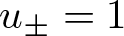 $u_{\pm}=1$. ν is a positive constant which characterizes the effect of the linear dispersion and the function
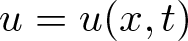 $u=u(x,t)$ is a function of time variable t and spatial variable x. The subscripts x and t appended to the functions m and u mean the partial differentiation of them.
Equation (Equation 1.3) was initially introduced by Fokas [Reference Fokas14]. Later on, the Lax integrability bi-Hamiltonian structure and conservation laws of it was firstly proposed by Qiao, Xia, and Li [Reference Xia, Qiao and Li44]. Subsequently, Wang and Qiao [Reference Wang and Qiao43] established the RH problem of the FQXLmodel
 \begin{equation}\textstyle m_t=\frac12k_1{\left[m\left(u^2-u_x^2\right)\right]}_x+\frac12k_2\left(2mu_x+m_xu\right),\;m=u-u_{xx},\end{equation}
which is in fact equivalent to Eq. (Equation 1.3) when letting 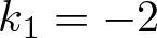 $k_1=-2$ and
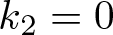 $k_2=0$. The RH problem with some important properties of the cCH equation has been investigated in references [Reference Xu and Fan46, Reference Yang and Fan48], then by adopting nonlinear steepest descent method and
 $\bar{\partial}$ steepest descent method, the long-time asymptotic behaviours of the solution with Schwartz initial data and weighted Sobolev initial data have been studied respectively. In an effort to obtain more properties of soliton solutions, this article goes deeply into the high-order pole solutions for the cCH equation based on the RH problem constructed in these two references. Due to the high-order negative powers at the poles, particularly for negative order equations, it can be challenging to construct solutions using general residue conditions. So this issue has not yet been fully resolved. Additionally, studying high-order solitons and high-order dispersion in relation to the cCH equation can lead to the discovery of new phenomena and important properties, making it a research area of great significance.
The inverse scattering transform (IST) method was introduced as a specialized calculation adapted to the initial-value problem for the KdV equation [Reference Chu and Scott10]. Through extended by some researchers, it can be used to solve the Fourier transform [Reference Ablowitz, Kaup, Newell and Segur2, Reference Gardner, Greene, Kruskal and Miura20, Reference Zakharov and Shabat49]. This method has been recognized as an important tool for solving various problems in mathematics, physics, and other fields. Meanwhile, it is particularly useful in obtaining the exact solutions for nonlinear wave equations by performing a series of linear computations. The RH problem, as a simplified modern version of IST, is a forceful tool to deal with the initial-boundary value problems of integrable systems. Its characteristic is that the solution of the corresponding RH problem can recover the reconstruction formula of the solution to the differential equation. There are numerous equations solved by RH approach when the space variable of solutions approach to zero or nonzero constant at infinities. Such as, the nonlinear Schrödinger (NLS) equation [Reference Biondini and Kovačič4, Reference Tian40, Reference Yang and Fan47], the coupled modified KdV equation [Reference Ji and Zhu24, Reference Ma28, Reference Tian41], the derivative NLS equation [Reference Zhang and Fan51], the nonlocal reverse-space-time NLS equation [Reference Ablowitz, Feng, Luo and Musslimani1], and the nonlocal real reverse-space-time mKdV equation [Reference Ma29].
The production and propagation of solitons play a crucial role in optical fiber communication. It is well-known that high-order soliton solutions are primarily obtained from high-order poles. The high-order soliton can be applied to describe a weak bound state of solitons and may appear in the study of train propagation of solitons with almost equivalent velocities and amplitudes. Therefore, studying high-order solitons and high-order dispersion is of utmost importance in this field. Taking advantage the RH method, through a standard dressing procedure, the soliton matrices of the high-order poles for the third-order flow Gerdjikov–Ivanov equation are constructed in [Reference Zhu and Chen52]. Nevertheless, when dealing with the RH problem with N-order poles, it is necessary to clearly give the corresponding residue conditions which are very complex and difficulty.
Recently, a new method can solve the RH problem with high-order poles are developed [Reference Zhang, Qiu and He50]. By using Laurent expansion and Taylor series, we generalize the residue theorem and get out of the complicated calculations, then the multiple high-order pole solitons are established. Hence, comparing to the work of [Reference Wang and Qiao43], we not only provide the multi-soliton solutions of (Equation 1.3) but also consider the multiple high-order pole solutions with both ZBCs and NZBCs. In addition to study Ablowitz-Kaup-Newell-Suger (AKNS) hierarchy, we extend the RH method to study the non-AKNS-typeintegrable cCH equation with ZBCs and NZBCs and give the exact expressions of soliton solutions with one high-order pole and multiple high-order poles. We generalize the results presented in [Reference Boutet de Monvel, Karpenko and Shepelsky5] after taking into account the impact of additional a linear dispersion term  $\nu u_{x}$. The Lax pair in [Reference Boutet de Monvel, Karpenko and Shepelsky5] is the simplest special case of our Lax pair. When the parameter ν is equal to zero and the orders of the poles are all equal to one, the solutions we obtained under NZBCs can degenerate into the solution in [Reference Boutet de Monvel, Karpenko and Shepelsky5]. These distinctions make our work more general and involve more complex analysis. It is worth noting that there are some differences from that on cCH equation (Equation 1.2) as mentioned in the following aspects.
(I) Since the cCH equation we have researched has a linear dispersion term
 $\nu u_{x}$, the Lax pair has a more complex form regarding the negative power of spectral parameter. Especially for the NZBCs, due to the deformation of the potential function, the Lax pair undergoes corresponding deformation as well. Then the suitable uniformization variable µ should be introduced. This gives rise to new spectral singularities that pose challenges for subsequent analysis.
(II) The cCH equation belongs to the family of negative-order equations and the uniformization variable µ is introduced, there are some singularities in the Lax pair. Under ZBCs, the cCH equation exhibits singularities at points µ = 0,
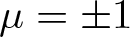
$\mu=\infty$ and branch cut points $\mu=\pm i$. Under NZBCs, new singularities arise at points $\mu=\pm1$. Analysing the asymptotic properties of these points is crucial because they significantly impact the construction of the RH problem.(III) Under NZBCs, based on the relationship
$y(x,t)=x-\int_{x}^{+\infty}(\hat{m}(\xi,t)-1)d\xi$ between variables x and y and considering the condition $\hat{X}_{0}(x,t,\pm i)\equiv0$, we study the scattering data $a(\mu)$ and $b(\mu)$ about the above relationship. Then the implicit expression of the potential function u is given by the solution of RH problem.(IV) Under NZBCs, in order to give the explicit expression of the potential function u of cCH equation, we need to use the compatibility condition
$\tilde{U}_{t}-\tilde{V}_{y}+[\tilde{U},\tilde{V}]=0$ and expand $\tilde{U}$, $\tilde{V}$ at singular points.(V) The function
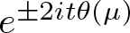
$a(\mu)$ is a Wronskian of analytic Jost solutions, which vanishes to N-order at the N-order zero points, we obtain a linear expression for the Nth derivative of Jost solutions. Then by utilizing Laurent expansion of $e^{\pm 2it\theta(\mu)}$, the multiple high-order pole solutions of cCH equation under ZBCs and NZBCs are established.

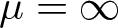
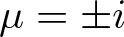







The outline of this work is arranged as follows. In §2, the spectrum problem of the cCH equation with ZBCs is analysed in detail. By introducing the Jost solutions, the analytical, asymptotic, and symmetric properties are gained. The cCH equation has singularities at points µ = 0, 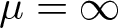 $\mu=\infty$, and
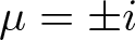 $\mu=\pm i$, through introducing suitable transformations to research these singularities, we can construct RH problem by a new scale (y, t) and recover the potential function at point
 $\mu=i$. Then, the expression of the solution with one N-order pole and multiple N-order poles are given, respectively. Finally, we give some examples analysing the dynamic behaviours of one-soliton solutions and two-order pole solutions. We compare the solution obtained by the RH method and the bilinear method, providing the expression for the solutions, and analysing them in conjunction with the figures.
In §3, by the same processing method, the RH problem of the cCH equation with NZBCs is established. Note that in addition to the above singularities, the points 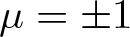 $\mu=\pm 1$ also are singularities, we need to consider the asymptotic properties of the eigenfunctions and scattering data at points
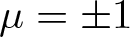 $\mu=\pm 1$. After that, the uniqueness of the solution about cCH equation with the new scale (y, t) is given. On the basis of proving the theory that the data of the RH problem are independent of some specific initial data of the cCH equation, we give the parametric representation of the solution. Finally, the expression of the solutions with one N-order pole and multiple N-order poles are derived, respectively. Furthermore, we analyse the dynamic behaviours of solutions by selecting special parameters.
2. RH problem and high-order pole under ZBCs
2.1. Spectral analysis
It is well-known that cCH equation (Equation 1.3) admits the following Lax pair
 \begin{align}
\phi_{x}=U\phi,\quad \phi_{t}=V\phi,
\end{align}
where  $U=U(x,t;\lambda)$ and
 $V=V(x,t;\lambda)$ are
 $2\times2$ matrices defined by
 \begin{align}
U=\left(\begin{array}{cc}
-\frac{Q}{2} & \frac{\lambda m}{2} \\
-\frac{\lambda m}{2} & \frac{Q}{2}
\end{array}\right),\quad
V=\left(\begin{array}{cc}
\frac{Q}{\lambda^{2}}+\frac{QR}{2} & -\frac{u-Qu_x}{\lambda}-\frac{\lambda Rm}{2} \\
\frac{u+Qu_x}{\lambda}+\frac{\lambda Rm}{2} & -\frac{Q}{\lambda^{2}}-\frac{QR}{2}
\end{array}\right),
\end{align}
with
 \begin{equation}
Q=Q(\nu,\lambda)=\sqrt{1-\frac{\nu\lambda^2}{2}},\ \ \ \ \ \ \
R=u^2-u_x^2.
\end{equation}
It can be seen that under the following transformations
 \begin{equation}
x=\tilde{x}, \quad t=\frac{2}{\nu}\tilde{t}, \quad
u(x,t)=\sqrt{\frac{\nu}{2}}\tilde{u}(\tilde{x},\tilde{t}),
\end{equation}
Eq. (Equation 1.3) turns to
 \begin{equation}
\tilde{m}_{\tilde{t}}+(\tilde{m} \tilde{R})_{\tilde{x}}+2\tilde{u}_{\tilde{x}}=0, \quad
\tilde{m}=\tilde{u}-\tilde{u}_{\tilde{x} \tilde{x}}, \quad \tilde{R}=\tilde{u}^2-\tilde{u}_{\tilde{x}}^2.
\end{equation}
Without loss of generality, we pick ν = 2. To get rid of the multi-value problem of square roots, we introduce a new transformation
 \begin{equation}
Q=\frac{i}{2}(\mu-\frac{1}{\mu}), \quad
\lambda=\frac{1}{2}(\mu+\frac{1}{\mu}).
\end{equation}
After doing a gauge transformation
 \begin{equation}
\psi=P^{-1}\phi e^{J},
\end{equation}
with
 \begin{equation}
P=P(x,t)=\sqrt{\frac{q+1}{2q}}
\left(\begin{array}{cc}
1 & -\frac{im}{q+1} \\
-\frac{im}{q+1} & 1
\end{array}\right),
\end{equation}
 \begin{equation}
\delta=x-\int_{x}^{+\infty}(q-1)dy-\frac{2t}{\lambda^2},
\quad q=\sqrt{m^2+1},
\end{equation}
where we define 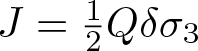 $J=\frac{1}{2}Q\delta\sigma_3$. The asymptotic condition is shown as follows
 \begin{align*}
\psi(x,t,\mu)\sim I,\quad x\rightarrow\pm\infty.
\end{align*}
Equation (Equation 1.3) has the following form Lax pair
 \begin{align}
&\psi_x+[J_x,\psi]=X\psi,
\end{align}
 \begin{align}
&\psi_t+[J_t,\psi]=T\psi,
\end{align}
where
 \begin{equation*}
X=\frac{im_x}{2q^2}\sigma_1+\frac{m}{2\mu q}
\left(\begin{array}{cc}
-im & 1 \\
-1 & im
\end{array}\right),\nonumber
\end{equation*}
 \begin{equation*}
\begin{split}
T=&\frac{im_t}{2q^2}\sigma_1-\frac{mR}{2\mu q}
\left(\begin{array}{cc}
-im & 1 \\
-1 & im
\end{array}\right)
+\frac{(\mu^2-1)u_x}{\mu^2+1}\sigma_1-\frac{2 \mu u}{(\mu^2+1)q}
\left(\begin{array}{cc}
-im & 1 \\
-1 & im
\end{array}\right) \\
&+\frac{2i\mu(\mu^2-1)}{(\mu^2+1)^2}
\left(\begin{array}{cc}
\frac{1}{q}-1 & -\frac{im}{q} \\
\frac{im}{q} & 1-\frac{1}{q}
\end{array}\right),\nonumber
\end{split}
\end{equation*}
there  $[A,B]=AB-BA$ and the notations
 $J=J(x,t,\mu)$,
 $X=X(x,t,\mu)$,
 $T=T(x,t,\mu)$ are
 $2\times2$ matrices. The σ 1 is Pauli matrix and the Pauli matrices are that
 \begin{equation*}
\sigma_1=
\left(\begin{array}{cc}
0 & 1 \\
1 & 0
\end{array}\right),\quad
\sigma_2=
\left(\begin{array}{cc}
0 & -i \\
i & 0
\end{array}\right),\quad
\sigma_3=
\left(\begin{array}{cc}
1 & 0 \\
0 & -1
\end{array}\right). \nonumber
\end{equation*}
The two Jost solutions of (Equation 2.10a) are completely determined by Volterra integrable equations
 \begin{equation}
\psi_\pm(x,t,\mu)=I+\int_{\pm\infty}^{x}e^{-\frac{i}{4}(\mu-\frac{1}{\mu})
\int_{y}^{x}qd\tau \hat{\sigma}_3}\left[X(y,t,\mu)\psi_\pm(y,t,\mu)\right]dy,
\end{equation}
where  $e^{A\hat{\sigma}_{3}}B=e^{A\sigma_{3}}Be^{-A\sigma_{3}}$. They have the analytic properties, symmetry properties, and asymptotic properties shown in the following three propositions.
Proposition 2.1. Providing that  $u_{0}(x)\in L^{1}({\mathbb{R}}^{\pm})$, the Jost eigenfunctions
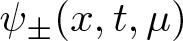 $\psi_{\pm}(x,t,\mu)$ have the following analytic properties, that is,
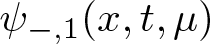 $\psi_{-,1}(x,t,\mu)$ and
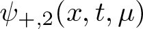 $\psi_{+,2}(x,t,\mu)$ are analytic in
 $\mathbb{C}^{+}$,
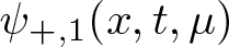 $\psi_{+,1}(x,t,\mu)$ and
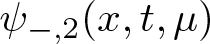 $\psi_{-,2}(x,t,\mu)$ are analytic in
 $\mathbb{C}^{-}$, there
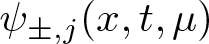 $\psi_{\pm,j}(x,t,\mu)$ (
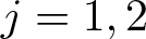 $j=1,2$) represent the j-th column of
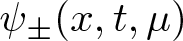 $\psi_{\pm}(x,t,\mu)$,
 $\mathbb{C}^{+}=\{\mu\in\mathbb{C}|Im\mu \gt 0\}$ and
 $\mathbb{C}^{-}=\{\mu\in\mathbb{C}|Im\mu \lt 0\}$.
Proposition 2.2. The Jost eigenfunctions 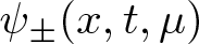 $\psi_{\pm}(x,t,\mu)$ have the following symmetry conditions
 \begin{equation}
\psi_{\pm}(\mu)=\sigma_1\psi_{\pm}^{*}
(-\frac{1}{\mu^{*}})\sigma_1=\sigma_2\psi_{\pm}^{*}
(\mu^{*})\sigma_2=\frac{1}{P^{2}}\sigma_2\psi_{\pm}(-\frac{1}{\mu})\sigma_2.
\end{equation}
Proposition 2.3. The Jost eigenfunctions 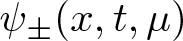 $\psi_{\pm}(x,t,\mu)$ possess asymptotic behaviour in the µ-plane
 \begin{equation}
\psi_{\pm}(x,t,\mu)=I+\mathcal {O}(\frac{1}{\mu}),\quad \mu\rightarrow\pm\infty,
\end{equation}
and according to the symmetry relations of 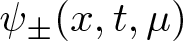 $\psi_{\pm}(x,t,\mu)$, there are the same relations when
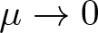 $\mu\rightarrow 0$.
It can be seen that 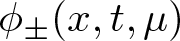 $\phi_{\pm}(x,t,\mu)$ are two fundamental matrix solutions of Lax pair (Equation 2.1). As a result, there exists a matrix
 $S(\mu)$ which independent of variables x and t satisfies
 \begin{equation}
\phi_-(x,t,\mu)=\phi_+(x,t,\mu)S(\mu),
\end{equation}
then on the basis of transformation (Equation 2.7), the relation (Equation 2.14) can be written in the following form
 \begin{equation}
\psi_-(x,t,\mu)e^{-J(x,t,\mu)}=\psi_+(x,t,\mu)e^{-J(x,t,\mu)}S(\mu),
\end{equation}
where  $S(\mu)$ is a
 $2\times2$ matrix. We can derive the symmetries of
 $S(\mu)$ from proposition 2.2 as follows
 \begin{equation}
S(\mu)=S^{*}(\frac{1}{\mu^{*}})=\sigma_3S(-\frac{1}{\mu})\sigma_3
=\sigma_{2}S^{*}(\mu^{*})\sigma_{2}.
\end{equation}
According to symmetry relation (Equation 2.12), we can define the matrix  $S(\mu)$ as the following form
 \begin{equation}
S(\mu)=\left(\begin{array}{cc}
a(\mu) & -b^{*}(\mu^{*}) \\
b(\mu) & a^{*}(\mu^{*})
\end{array}\right).
\end{equation}
Because 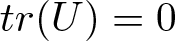 $tr(U)=0$, based on Abel theorem, we have
 $\det(\psi_{\pm})=1$, then
 $\det(S(\mu))=1$. By directly calculating Eq. (Equation 2.15),
 $a(\mu)$ and
 $b(\mu)$ can be expressed as
 \begin{equation}
a(\mu)=Wr(\psi_{-1},\psi_{+2}), \quad b(\mu)=Wr(\psi_{+1},\psi_{-1}).
\end{equation}
We define the reflection coefficient
 \begin{equation}
\rho(\mu)=\frac{b(\mu)}{a(\mu)}.
\end{equation}
Taking into account the properties of the Jost eigenfunctions 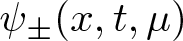 $\psi_{\pm}(x,t,\mu)$, we obtain the corresponding properties to the elements
 $a(\mu)$ and
 $b(\mu)$ of the scattering matrix
 $S(\mu)$ as follows.
Proposition 2.4. The scattering data  $a(\mu)$ and
 $b(\mu)$ satisfy the following properties
(i)
$a(\mu)$ can be analytically continued in ${\mathbb{C}}^{+}$, and $b(\mu)$ is continuous in $\mathbb{R}$;(ii)
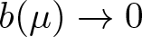
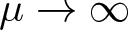
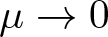
$a(\mu)=1+\mathcal {O}(\frac{1}{\mu})$ and $b(\mu)\rightarrow 0$ as $\mu \rightarrow \infty$, and from the symmetry relations of $\psi_{\pm}(x,t,\mu)$, there are the same relations when $\mu\rightarrow 0$;(iii) the reflection coefficient
$\rho(\mu)$ possesses the symmetry relations
(2.20)\begin{equation}
\rho(\mu)=\rho^{*}(\frac{1}{\mu^{*}})=-\rho(-\frac{1}{\mu})
=-\rho^{*}(-\mu^{*}).
\end{equation}



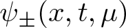


It is noticed that, since the branch cut points 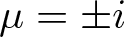 $\mu=\pm i$ exist in the extended complex µ-plane, the asymptotic behaviour of eigenfunctions
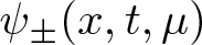 $\psi_{\pm}(x,t,\mu)$ ought to be considered as
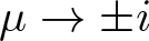 $\mu\rightarrow \pm i$. Introducing a new Jost function
 \begin{equation}
\tilde{\psi}_{\pm}(x,t,\mu)=\phi_{\pm}(x,t,\mu)
e^{(\frac{Q}{2}x-\frac{Q}{\lambda^{2}}t)\sigma_{3}},
\end{equation}
then we have
 \begin{equation}
\tilde{\psi}_{\pm}(x,t,\mu)\sim I,\quad x\rightarrow\pm \infty.
\end{equation}
The Lax pair (Equation 2.1) can be converted to
 \begin{align}
&(\tilde{\psi}_{\pm})_{x}=-\frac{Q}{2}[\sigma_{3},\tilde{\psi}_{\pm}]
+\tilde{X}\tilde{\psi}_{\pm},
\end{align}
 \begin{align}
&(\tilde{\psi}_{\pm})_{t}=\frac{Q}{\lambda^{2}}[\sigma_{3},\tilde{\psi}_{\pm}]
+\tilde{T}\tilde{\psi}_{\pm},
\end{align}
with
 \begin{align*}
&\tilde{X}=
\left(\begin{array}{cc}
0 & \frac{\lambda m}{2} \\
-\frac{\lambda m}{2} & 0
\end{array}\right),\\
&\tilde{T}=\frac{R}{2}
\left(\begin{array}{cc}
Q & -\lambda m \\
\lambda m & -Q
\end{array}\right)+\frac{u-Qu_{x}}{\lambda}
\left(\begin{array}{cc}
0 & -1 \\
1 & 0
\end{array}\right).
\end{align*}
Taking into account the asymptotic expansion of  $\tilde{\psi}$ at
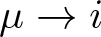 $\mu\rightarrow i$, we have
 \begin{equation}
\tilde{\psi}=I+\tilde{\psi}_{1}(\mu-i)+\mathcal {O}((\mu-i)^{2}),
\quad \mu\rightarrow i,
\end{equation}
with
 \begin{equation}
\tilde{\psi}_{1}=
\left(\begin{array}{cc}
0 & -\frac{1}{2}(u+u_{x}) \\
-\frac{1}{2}(u-u_{x}) & 0
\end{array}\right).
\end{equation}
According to the transformations (Equation 2.7) and (Equation 2.21), we have
 \begin{equation}
\psi_{\pm}(x,t,\mu)=P^{-1}(x,t)\tilde{\psi}_{\pm}(x,t,\mu)
e^{\frac{1}{2}Q(\mu)\int_{\pm\infty}^{x}(q-1)dy}.
\end{equation}
Taking the limits of (Equation 2.26) as 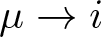 $\mu \rightarrow i $, we obtain the asymptotic of
 $a(\mu)$
 \begin{equation}
a(\mu)=e^{-\frac{1}{2}\int_{-\infty}^{+\infty}(q-1)dx}(1+\mathcal {O}((\mu-i)^{2})),
\quad \mu\rightarrow i.
\end{equation}
The analytic properties of 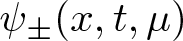 $\psi_{\pm}(x,t,\mu)$ stated above allow rewriting the relation (Equation 2.15) as a sectionally meromorphic matrix.
2.2. RH problem
Define a piecewise meromorphic  $2\times2$-matrix valued function
 \begin{align}
M(\mu)=M(x,t;\mu):=\left\{\begin{array}{ll}
\left( \frac{\psi_{-,1}(x,t;\mu)}{a(\mu)}, \psi_{+,2}(x,t;\mu)\right), &\text{as } \mu\in \mathbb{C}^+,\\[12pt]
\left( \psi_{+,1}(x,t;\mu),\frac{\psi_{-,2}(x,t;\mu)}{a^{*}(\mu^{*})}\right) , &\text{as }\mu\in \mathbb{C}^-.
\end{array}\right.
\end{align}
RHP 2.5.
Find a matrix  $M(\mu)=M(x,t,\mu)$ satisfies the following conditions
(i) Analyticity: the matrix
$M(\mu)$ is a meromorphic function in $\mathbb{C}\backslash\mathbb{R}$.(ii) Asymptotic behaviour:
(2.29)\begin{align}
&M(\mu)=I+\mathcal {O}(\frac{1}{\mu}),\quad \mu\rightarrow\infty,
\end{align}(2.30)\begin{align}
&M(\mu)=P^{-1}[I+\tilde{\psi}_{1}(\mu-i)]e^{\frac{1}{2}\int_{+\infty}^{x}(q-1)dy\sigma_3}
+\mathcal {O}((\mu-i)^{2}),\quad \mu\rightarrow i.
\end{align}(iii) Jump condition:
(2.31)\begin{align}
M_{+}(\mu)=M_{-}(\mu)G(\mu),\quad \mu\in\mathbb{R},
\end{align}where
(2.32)\begin{align}
G(\mu)=\left(\begin{array}{cc}
1+|\rho(\mu)|^{2} & e^{-Q\delta}\rho^{*}(\mu)\\
e^{Q\delta}\rho(\mu) & 1
\end{array}\right).
\end{align}(iv) Symmetries:
$M(\mu)=\sigma_3M^{*}(-\mu^{*})\sigma_3$=$\sigma_2M^{*}(\mu^{*})
\sigma_2=P^{-2}\sigma_{1}M^{*}(-\frac{1}{\mu^{*}})\sigma_{1}$.




Since the function 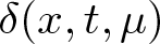 $\delta(x,t,\mu)$ has integral term, which directly lead to the difficulty to solve Eq. (Equation 1.3), a new space variable is introduced as follows
 \begin{equation}
y(x,t)=x-\int_{x}^{+\infty}(q(s,t)-1)ds.
\end{equation}
Defining the function  $\tilde{M}(\mu)$ and phase function
 $\theta(\mu)$ on the new scale
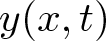 $y(x,t)$
 \begin{equation}
\tilde{M}(\mu)=\tilde{M}(y,t,\mu)=M(x(y,t),t,\mu),
\end{equation}
 \begin{equation}
\theta(\mu)=\frac{1}{2}iQ(\mu)\left(\frac{y}{t}-\frac{2}{\lambda^{2}(\mu)}\right),
\end{equation}
then, the RH problem 2.5 is transformed as follows.
RHP 2.6.
Find a matrix  $\tilde{M}(\mu)=\tilde{M}(y,t,\mu)$ satisfies the following conditions
(i) Analyticity: the matrix
$\tilde{M}(\mu)$ is a meromorphic function in $\mathbb{C}\backslash\mathbb{R}$.(ii) Asymptotic behaviour:
(2.36)\begin{align}
&\tilde{M}(\mu)=I+\mathcal {O}(\frac{1}{\mu}),\quad \mu\rightarrow\infty,
\end{align}(2.37)\begin{align}
&\tilde{M}(\mu)=P^{-1}[I+\tilde{\psi}_{1}(\mu-i)]e^{\frac{1}{2}\int_{+\infty}^{x}(q-1)dy\sigma_3}
+\mathcal {O}((\mu-i)^{2}),\quad \mu\rightarrow i.
\end{align}(iii) Jump condition:
(2.38)\begin{align}
\tilde{M}_{+}(\mu)=\tilde{M}_{-}(\mu)V(\mu),\quad \mu\in\mathbb{R},
\end{align}where
(2.39)\begin{align}
V(\mu)=\left(\begin{array}{cc}
1+|\rho(\mu)|^{2} & e^{2it\theta(\mu)}\rho^{*}(\mu)\\
e^{-2it\theta(\mu)}\rho(\mu) & 1
\end{array}\right).
\end{align}(iv) Symmetries:
$\tilde{M}(\mu)=\sigma_3\tilde{M}^{*}(-\mu^{*})\sigma_3$=$\sigma_2\tilde{M}^{*}(\mu^{*})
\sigma_2=P^{-2}\sigma_{1}\tilde{M}^{*}(-\frac{1}{\mu^{*}})\sigma_{1}$.




Using the asymptotic property of function  $\tilde{M}(\mu)$ as
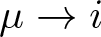 $\mu\rightarrow i$, the relationship between the solution of cCH equation and the RH problem is obtained
 \begin{equation}
u(x,t)=\lim_{\mu \to i}\frac{1}{\mu-i}\left(1-\frac{(\tilde{M}_{11}(\mu)+\tilde{M}_{21}(\mu))
(\tilde{M}_{12}(\mu)+\tilde{M}_{22}(\mu))}
{(\tilde{M}_{11}(i)+\tilde{M}_{21}(i))(\tilde{M}_{12}(i)+\tilde{M}_{22}(i))}\right),
\end{equation}
with
 \begin{equation}
x(y,t)=
y-\ln\left(\frac{\tilde{M}_{12}(i)+\tilde{M}_{22}(i)}{\tilde{M}_{11}(i)+\tilde{M}_{21}(i)}\right),
\end{equation}
where 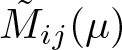 $\tilde{M}_{ij}(\mu)$
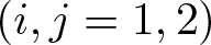 $(i,j=1,2)$ represents the element in raw i and column j of
 $\tilde{M}(\mu)$.
2.3. Single high-order pole solutions
In order to obtain a pure soliton solution, this section we will consider the reflectionless situation, i.e., 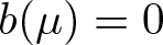 $b(\mu)=0$. Then
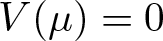 $V(\mu)=0$ for
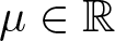 $\mu\in\mathbb{R}$. We assume that
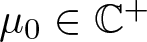 $\mu_{0}\in\mathbb{C}^{+}$ is the only one N-order zero point of the scattering data
 $a(\mu)$, then the N-order zero points
 $\left\{-\mu^{*}_{0}, -\frac{1}{\mu_{0}}, \frac{1}{\mu^{*}_{0}}\right\}\in
\mathbb{C}^{+}$ are also obtained from the symmetry of
 $a(\mu)$. Additionally,
 $\left\{\mu^{*}_{0}, -\mu_{0}, -\frac{1}{\mu^{*}_{0}}, \frac{1}{\mu_{0}}\right\}\in\mathbb{C}
^{-}$ are the N-order zero points of the scattering data
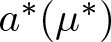 $a^{*}(\mu^{*})$.
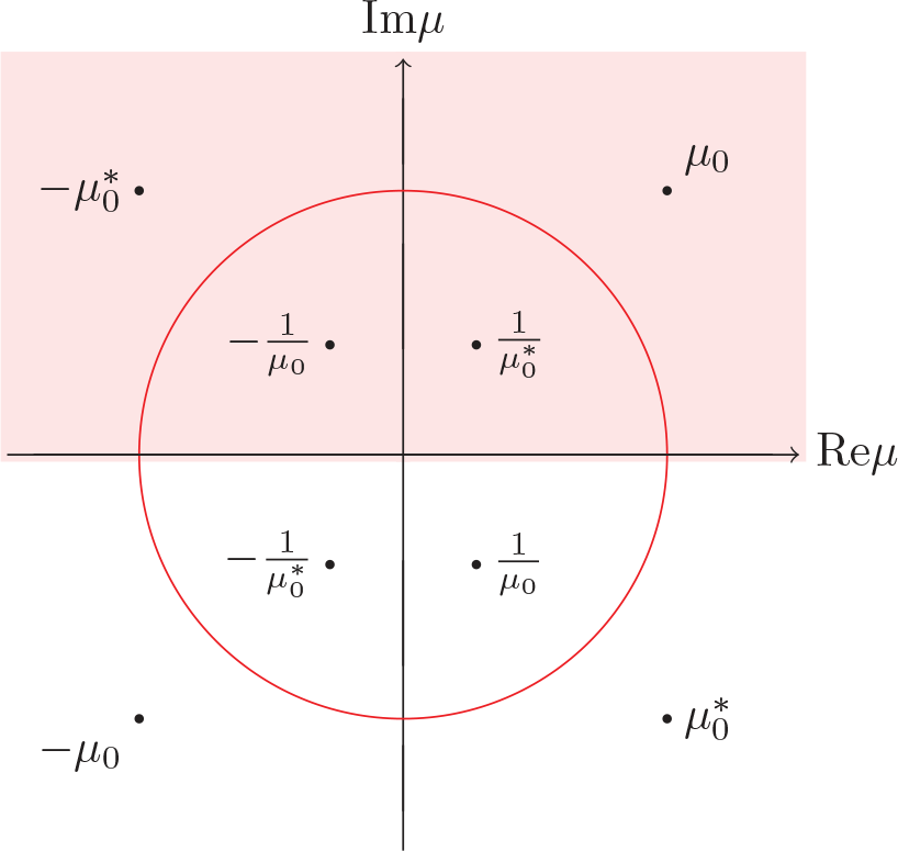
The discrete spectrum is the set  $\mathcal{Z}=\left\{\pm\mu_{0}, \pm\mu^{*}_{0}, \pm\frac{1}{\mu_{0}}, \pm\frac{1}{\mu^{*}_{0}}\right\}$, which can be shown in Figure 1. After taking
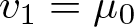 $v_{1}=\mu_{0}$,
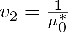 $v_{2}=\frac{1}{\mu^{*}_{0}}$, the scattering data
 $a(\mu)$ can be expressed as
 \begin{equation}
a(\mu)=\prod_{j=1}^{2}(\mu-v_{j})^{N}(\mu+v^{*}_{j})^{N}a_{0}(\mu),
\end{equation}
Distribution of the discrete spectrum  $\mathcal{\mu}$.

where 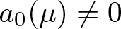 $a_{0}(\mu)\neq0$ for all
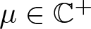 $\mu\in\mathbb{C}^{+}$. Therefore, from the definition of
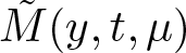 $\tilde{M}(y,t,\mu)$, it can be seen that
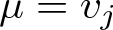 $\mu=v_{j}$ and
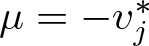 $\mu=-v^{*}_{j}$
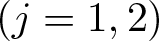 $(j=1,2)$ are N-order pole points of
 $\tilde{M}_{11}$. Simultaneously,
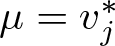 $\mu=v^{*}_{j}$ and
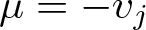 $\mu=-v_{j}$
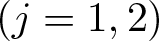 $(j=1,2)$ are N-order pole points of
 $\tilde{M}_{12}$.
Based on the definitions of (Equation 2.14) and (Equation 2.15), under the new scale 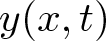 $y(x,t)$, we define
 $\breve{\phi}_{\pm}(y,t,\mu)=\phi_{\pm}(x,t,\mu)$ and
 $\breve{\psi}_{\pm}(y,t,\mu)=\psi_{\pm}(x,t,\mu)$ and obtain the following relationships
 \begin{equation}
\breve{\phi}_-(y,t,\mu)=\breve{\phi}_+(y,t,\mu)S(\mu),
\end{equation}
and
 \begin{equation}
\breve{\psi}_-(y,t,\mu)e^{it\theta(\mu)\sigma_{3}}=\breve{\psi}_+(y,t,\mu)e^{it\theta(\mu)\sigma_{3}}S(\mu),
\end{equation}
where  $\theta(\mu)$ is defined in (Equation 2.35). Under the assumption that
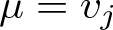 $\mu=v_{j}$
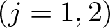 $(j=1,2)$ are N-order zero points of
 $a(\mu)$, from the following two relations,
 $a(\mu)$ can be represented as a Wronskian of analytic Jost solutions
 \begin{equation}
a(\mu)=Wr(\breve{\phi}_{-1},\breve{\phi}_{+2}),
\end{equation}
then at zero points vj 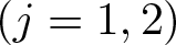 $(j=1,2)$,
 $a(\mu)$ vanishes to N-order, there exist complex constants
 $b_{j,s}$
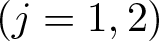 $(j=1,2)$
 $(s=1,2,\cdots,N)$ satisfy the follows
 \begin{equation}
\frac{\partial^{m}[\breve{\phi}_+(y,t,v_{j})]_{2}}{\partial\mu^{m}}=\sum^{m}_{l=0}\left(\begin{array}{c}
m \\
l
\end{array}\right)
b_{j,m-l+1}\frac{\partial^{l}[\breve{\phi}_-(y,t,v_{j})]_{1}}{\partial\mu^{l}},
\end{equation}
and
 \begin{equation}
\frac{\partial^{m}[\breve{\psi}_+(y,t,v_{j})]_{2}}{\partial\mu^{m}}=\sum^{m}_{l=0}\left(\begin{array}{c}
m \\
l
\end{array}\right)
b_{j,m-l+1}\frac{\partial^{l}[\breve{\psi}_-(y,t,v_{j})]_{1}e^{2it\theta(v_{j})}}{\partial\mu^{l}},
\end{equation}
with  $m=0,1,\cdots,N-1$.
On the basis of the definition of  $M(\mu)$ defined by (Equation 2.28) and the asymptotic behaviour in RH problem 2.6, we set
 \begin{align}
&\tilde{M}_{11}(y,t,\mu)=1+\sum_{j=1}^{2}\sum_{s=1}^{N}
\left(\frac{1}{(\mu-v_{j})^{s}}+\frac{(-1)^{s}}{(\mu+v^{*}_{j})^{s}}\right)F_{j,s}(y,t),
\end{align}
 \begin{align}
&\tilde{M}_{12}(y,t,\mu)=\sum_{j=1}^{2}\sum_{s=1}^{N}
\left(\frac{1}{(\mu-v^{*}_{j})^{s}}+\frac{(-1)^{s+1}}{(\mu+v_{j})^{s}}\right)G_{j,s}(y,t),
\end{align}
where 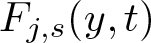 $F_{j,s}(y,t)$ and
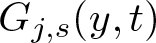 $G_{j,s}(y,t)$ are undetermined functions. Making use of Taylor series expansion, one can obtain the following relationships
 \begin{align}
&e^{-2it\theta(\mu)}=\sum_{l=0}^{+\infty}\zeta_{j,l}(y,t)(\mu-v_{j})^{l},\quad
e^{2it\theta(\mu)}=\sum_{l=0}^{+\infty}\zeta^{*}_{j,l}(y,t)(\mu-v^{*}_{j})^{l},
\end{align}
where the element 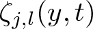 $\zeta_{j,l}(y,t)$ is
 \begin{align*}
\zeta_{j,l}(y,t)=\lim_{\mu\rightarrow v_{j}}\frac{1}{l!}\frac{\partial^{l}}{\partial \mu^{l}}e^{-2it\theta(\mu)},\quad
\zeta^{*}_{j,l}(y,t)=\lim_{\mu\rightarrow v^{*}_{j}}\frac{1}{l!}\frac{\partial^{l}}{\partial \mu^{l}}e^{2it\theta(\mu)}.
\end{align*}
It can be obtained that the coefficient of item 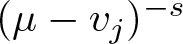 $(\mu-v_{j})^{-s}$ of function
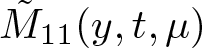 $\tilde{M}_{11}(y,t,\mu)$ is
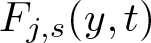 $F_{j,s}(y,t)$. Now we extend the residue theorem by combining (Equation 2.44) and (Equation 2.47) and obtain the following relations
 \begin{align}
\begin{split}
F_{j,s}&=\sum_{l=s}^{N}\sum_{m=0}^{l-s}\sum_{p=1}^{2}\sum_{q=1}^{N}
\left(
\begin{array}{c}
q+m-1\\
m \\
\end{array}
\right) \times \\
&r_{j,l}\zeta_{j,l-s-m}
\left\{\frac{(-1)^{m}}{(v_{j}-v^{*}_{p})^{q+m}}
+\frac{(-1)^{m+q+1}}{(v_{j}+v_{p})^{q+m}}\right\}G_{p,q},
\end{split}
\end{align}
where
 \begin{align}
r_{j,l}=\lim_{\mu\rightarrow v_{j}}\frac{b_{j,l}}{(N-l)!}\frac{\partial^{N-l}}{\partial(\mu-v_{j})^{N-l}}
\frac{(\mu-v_{j})^{N}}{a(\mu)}.
\end{align}
Likewise, the coefficient of item 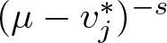 $(\mu-v^{*}_{j})^{-s}$ of function
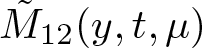 $\tilde{M}_{12}(y,t,\mu)$ is
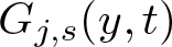 $G_{j,s}(y,t)$. Through the same method, we have
 \begin{align}
\begin{split}
G_{j,s}&=-\sum_{l=s}^{N}r^{*}_{j,l}\zeta^{*}_{j,l-s}
-\sum_{l=s}^{N}\sum_{m=0}^{l-s}\sum_{p=1}^{2}\sum_{q=1}^{N}
\left(
\begin{array}{c}
q+m-1\\
m \\
\end{array}
\right)\times\\
&r^{*}_{j,l}\zeta^{*}_{j,l-s-m}\left\{\frac{(-1)^{m}}
{(v^{*}_{j}-v_{p})^{q+m}}
+\frac{(-1)^{m+q}}{(v^{*}_{j}+v^{*}_{p})^{q+m}}\right\}F_{p,q}.
\end{split}
\end{align}
Introducing the new notations for 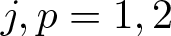 $j,p=1,2$
 \begin{align}
|\eta_{j}\rangle&=(\eta_{j1},\cdots,\eta_{jN})^{T},\quad
\eta_{js}=-\sum_{l=s}^{N}r^{*}_{j,l}\zeta^{*}_{j,l-s}(y,t),
\end{align}
then defining the N × N matrices  $\vartheta_{j,p}=[\vartheta_{j,p}]_{s,q}$ and
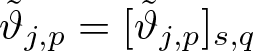 $\tilde{\vartheta}_{j,p}=[\tilde{\vartheta}_{j,p}]_{s,q}$ for
 $s,q=1,2,\cdots,N$ as follows
 \begin{align}
\begin{split}
\vartheta_{j,p}=\sum_{l=s}^{N}\sum_{m=0}^{l-s}
\left(
\begin{array}{c}
q+m-1\\
m \\
\end{array}
\right)
r_{j,l}\zeta_{j,l-s-m}\left\{\frac{(-1)^{m}}{(v_{j}-v^{*}_{p})^{q+m}}
+\frac{(-1)^{m+q+1}}{(v_{j}+v_{p})^{q+m}}\right\},
\end{split}
\end{align}
 \begin{align}
\begin{split}
\tilde{\vartheta}_{j,p}=\sum_{l=s}^{N}\sum_{m=0}^{l-s}
\left(
\begin{array}{c}
q+m-1\\
m \\
\end{array}
\right)
r^{*}_{j,l}\zeta^{*}_{j,l-s-m}\left\{\frac{(-1)^{m}}
{(v^{*}_{j}-v_{p})^{q+m}}
+\frac{(-1)^{m+q}}{(v^{*}_{j}+v^{*}_{p})^{q+m}}\right\},
\end{split}
\end{align}
 \begin{align}
|F_{p}\rangle=(F_{p,1},\cdots,F_{p,N})^{T},\quad
|G_{p}\rangle=(G_{p,1},\cdots,G_{p,N})^{T},
\end{align}
 \begin{align}
\vartheta=
\left(\begin{array}{cc}
\vartheta_{1,1} & \vartheta_{1,2} \\
\vartheta_{2,1} & \vartheta_{2,2}
\end{array}\right),\quad
\tilde{\vartheta}=
\left(\begin{array}{cc}
\tilde{\vartheta}_{1,1} & \tilde{\vartheta}_{1,2} \\
\tilde{\vartheta}_{2,1} & \tilde{\vartheta}_{2,2}
\end{array}\right),\quad
I_{\sigma}=
\left(\begin{array}{cc}
I & 0 \\
0 & I
\end{array}\right),
\end{align}
where I is a N × N identity matrix. Equations (Equation 2.50)–(Equation 2.52) can be written as a system of linear equations
 \begin{equation}
\begin{aligned}
&I|F_{p}\rangle-\vartheta_{j,p}|G_{p}\rangle=0,\\
&\tilde{\vartheta}_{j,p}|F_{p}\rangle+
I|G_{p}\rangle=|\eta_{j}\rangle.
\end{aligned}
\end{equation}
Then taking
 \begin{align}
|F\rangle=(|F_{1}\rangle,|F_{2}\rangle)^{T},\quad
|G\rangle=(|G_{1}\rangle,|G_{2}\rangle)^{T},
\end{align}
 \begin{align}
|\eta\rangle=(|\eta_{1}\rangle,|\eta_{2}\rangle)^{T}.
\end{align}
The system (Equation 2.58) has the following solution
 \begin{align}
|F\rangle=(I_{\sigma}+\vartheta\tilde{\vartheta})^{-1}\vartheta|\eta\rangle,\quad
|G\rangle=(I_{\sigma}+\tilde{\vartheta}\vartheta)^{-1}|\eta\rangle.
\end{align}
The new expression of (Equation 2.48a) is derived as
 \begin{align}
\tilde{M}_{11}(y,t,\mu)&=\frac{\det(I_{\sigma}+\vartheta\tilde{\vartheta}+|\eta\rangle\langle\Upsilon(\mu)|\vartheta)}
{\det(I_{\sigma}+\vartheta\tilde{\vartheta})},
\end{align}
 \begin{align}
\tilde{M}_{12}(y,t,\mu)&=\frac{\det(I_{\sigma}+\tilde{\vartheta}\vartheta+|\eta\rangle\langle\tilde{\Upsilon}(\mu)|)}
{\det(I_{\sigma}+\tilde{\vartheta}\vartheta)}-1,
\end{align}
with
 \begin{equation}
\begin{split}
&\langle\Upsilon(\mu)|=(\langle\Upsilon_{1}(\mu)|,\langle\Upsilon_{2}(\mu)|),\quad
\langle\Upsilon_{j}(\mu)|=(\Upsilon_{j1},\ldots,\Upsilon_{jN}),\\
&\langle\tilde{\Upsilon}(\mu)|
=(\langle\tilde{\Upsilon}_{1}(\mu)|,\langle\tilde{\Upsilon}_{2}(\mu)|),\quad
\langle\tilde{\Upsilon}_{j}(\mu)|=(\tilde{\Upsilon}_{j1},\ldots,\tilde{\Upsilon}_{jN}),\\
&\langle\Upsilon^{\prime}(\mu)|=
(\langle\Upsilon^{\prime}_{1}(\mu)|,\langle\Upsilon^{\prime}_{2}(\mu)|),\quad
\langle\Upsilon^{\prime}_{j}(\mu)|=(\Upsilon^{\prime}_{j1},\ldots,\Upsilon^{\prime}_{jN}),\\
&\langle\tilde{\Upsilon}^{\prime}(\mu)|
=(\langle\tilde{\Upsilon}^{\prime}_{1}(\mu)|,\langle\tilde{\Upsilon}^{\prime}_{2}(\mu)|),\quad
\langle\tilde{\Upsilon}^{\prime}_{j}(\mu)|=(\tilde{\Upsilon}^{\prime}_{j1},\ldots,\tilde{\Upsilon}^{\prime}_{jN}),
\end{split}
\end{equation}
 \begin{align*}
&\Upsilon_{js}=\frac{1}{(\mu-v_{j})^{s}}+\frac{(-1)^{s}}{(\mu+v^{*}_{j})^{s}},\quad
\tilde{\Upsilon}_{js}=\frac{1}{(\mu-v^{*}_{j})^{s}}+\frac{(-1)^{s+1}}{(\mu+v_{j})^{s}},\\
&\Upsilon^{\prime}_{js}=\frac{-s}{(\mu-v_{j})^{s+1}}+\frac{s(-1)^{s+1}}{(\mu+v^{*}_{j})^{s+1}},\quad
\tilde{\Upsilon}^{\prime}_{js}=\frac{-s}{(\mu-v^{*}_{j})^{s+1}}+\frac{s(-1)^{s}}{(\mu+v_{j})^{s+1}},
\end{align*}
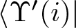
where we differentiate the components of vector 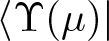 $\langle\Upsilon(\mu)|$ from variable µ to obtain vector
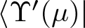 $\langle\Upsilon^{\prime}(\mu)|$, the vector
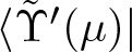 $\langle\tilde{\Upsilon}^{\prime}(\mu)|$ can also be gained from the same way. In the following content, we will continue to use this definition. On the basis of the symmetry of
 $\tilde{M}(\mu)=\sigma_2\tilde{M}^{*}(\mu^{*})\sigma_2$, we have
 \begin{align}
\tilde{M}_{22}(y,t,\mu)&=\frac{\det(I_{\sigma}+\tilde{\vartheta}^{*}\vartheta^{*}+|\eta^{*}\rangle\langle\Upsilon^{*}(\mu^{*})|\vartheta^{*})}
{\det(I_{\sigma}+\tilde{\vartheta}^{*}\vartheta^{*})},
\end{align}
 \begin{align}
\tilde{M}_{21}(y,t,\mu)&=-\frac{\det(I_{\sigma}+\vartheta^{*}\tilde{\vartheta}^{*}+|\eta^{*}\rangle\langle\tilde{\Upsilon}^{*}(\mu^{*})|)}
{\det(I_{\sigma}+\vartheta^{*}\tilde{\vartheta}^{*})}+1.
\end{align}
Hence the precise expression formula for the solution of cCH equation with single high-order pole under the ZBCs can be obtained in theorem 2.7.
Theorem 2.7
The solution of cCH equation with single high-order pole under the ZBCs can be obtained as follows
 \begin{align}
u(x,t)=-\left(
\frac{\tilde{M}^{\prime}_{11}(i)+\tilde{M}^{\prime}_{21}(i)}{\tilde{M}_{11}(i)+\tilde{M}_{21}(i)}+
\frac{\tilde{M}^{\prime}_{12}(i)+\tilde{M}^{\prime}_{22}(i)}{\tilde{M}_{12}(i)+\tilde{M}_{22}(i)}
\right),
\end{align}
with
 \begin{align*}
&\tilde{M}_{11}(i)=\frac{\det(I_{\sigma}+\vartheta\tilde{\vartheta}+|\eta\rangle\langle\Upsilon(i)|\vartheta)}
{\det(I_{\sigma}+\vartheta\tilde{\vartheta})},\\
&\tilde{M}_{21}(i)=-\frac{\det(I_{\sigma}+\vartheta^{*}\tilde{\vartheta}^{*}+|\eta^{*}\rangle\langle\tilde{\Upsilon}^{*}(-i)|)}
{\det(I_{\sigma}+\vartheta^{*}\tilde{\vartheta}^{*})}+1,\\
&\tilde{M}_{12}(i)=\frac{\det(I_{\sigma}+\tilde{\vartheta}\vartheta+|\eta\rangle\langle\tilde{\Upsilon}(i)|)}
{\det(I_{\sigma}+\tilde{\vartheta}\vartheta)}-1\\
&\tilde{M}_{22}(i)=\frac{\det(I_{\sigma}+\tilde{\vartheta}^{*}\vartheta^{*}+|\eta^{*}\rangle\langle\Upsilon^{*}(-i)|\vartheta^{*})}
{\det(I_{\sigma}+\tilde{\vartheta}^{*}\vartheta^{*})},\\
&\tilde{M}^{\prime}_{11}(i)=\frac{\det(I_{\sigma}+\vartheta\tilde{\vartheta}+|\eta\rangle\langle\Upsilon^{\prime}(i)|\vartheta)}
{\det(I_{\sigma}+\vartheta\tilde{\vartheta})}-1,\\
&\tilde{M}^{\prime}_{21}(i)=-\frac{\det(I_{\sigma}+\vartheta^{*}\tilde{\vartheta}^{*}+|\eta^{*}\rangle\langle\tilde{\Upsilon}^{\prime *}(-i)|)}
{\det(I_{\sigma}+\vartheta^{*}\tilde{\vartheta}^{*})}+1,\\
&\tilde{M}^{\prime}_{12}(i)=\frac{\det(I_{\sigma}+\tilde{\vartheta}\vartheta+|\eta\rangle\langle\tilde{\Upsilon}^{\prime}(i)|)}
{\det(I_{\sigma}+\tilde{\vartheta}\vartheta)}-1,\\
&\tilde{M}^{\prime}_{22}(i)=\frac{\det(I_{\sigma}+\tilde{\vartheta}^{*}\vartheta^{*}+|\eta^{*}\rangle\langle\Upsilon^{\prime *}(-i)|\vartheta^{*})}
{\det(I_{\sigma}+\tilde{\vartheta}^{*}\vartheta^{*})}-1,
\end{align*}
where 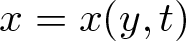 $x=x(y,t)$ is defined in (Equation 2.41), and the elements
 $|\eta\rangle$, Iσ, ϑ,
 $\tilde{\vartheta}$,
 $\langle\Upsilon(i)|$,
 $\langle\tilde{\Upsilon}(i)|$,
 $\langle\Upsilon^{\prime}(i)|$, and
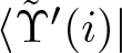 $\langle\tilde{\Upsilon}^{\prime}(i)|$ are respectively defined in (Equation 2.53), (Equation 2.57), and (Equation 2.64).
2.3.1. One-soliton solution
Next, we construct the simple one-soliton solution and compare the expressions of the solutions obtained by RH approach and Hirota’s bilinear method. In this case, the zero points of scattering data are one-order, and there is no need to calculate the high-order derivative formula of the Jost eigenfunctions and the complex Taylor expansions, which degenerates into the residue conditions of RH matrix. In order to compare with the solution obtained by bilinear method, we need to process the RH matrix and use the above construction process to obtain the simplest expression of solution.
For one-soliton solution, we have N = 1. Supposing 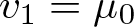 $v_{1}=\mu_{0}$ is a first-order zero point of the scattering data
 $a(\mu)$, then the symmetrical relationships indicate that
 $\left\{-\mu^{*}_{0}, -\frac{1}{\mu_{0}}, \frac{1}{\mu^{*}_{0}}\right\}\in\mathbb{C}^{+}$ also are zero points of
 $a(\mu)$. Then from Eqs. (Equation 2.44), (Equation 2.45), and (Equation 2.47), we use the symmetry relationships in RH problem 2.6 to calculate the following residue conditions
 \begin{align}
\begin{split}
\mathop{\operatorname{Res}}_{\mu=\mu_{0}}\tilde{M}^{(1)}(y,t,\mu)&=c_{0}e^{-2it\theta(\mu_{0})}\tilde{M}^{(2)}(y,t,\mu_{0}),\\
\mathop{\operatorname{Res}}_{\mu=\frac{1}{\mu^{*}_{0}}}\tilde{M}^{(1)}(y,t,\mu)&=-\frac{c^{*}_{0}}
{\mu^{*2}_{0}}e^{2it\theta^{*}(\mu_{0})}\tilde{M}^{(2)}(y,t,\frac{1}{\mu^{*}_{0}}),\\
\mathop{\operatorname{Res}}_{\mu=-\mu^{*}_{0}}\tilde{M}^{(1)}(y,t,\mu)&=-\frac{c_{0}}
{\mu^{2}_{0}}e^{2it\theta^{*}(\mu_{0})}\tilde{M}^{(2)}(y,t,-\mu^{*}_{0}),\\
\mathop{\operatorname{Res}}_{\mu=-\frac{1}{\mu_{0}}}\tilde{M}^{(1)}(y,t,\mu)&=-\frac{c_{0}}{\mu^{2}_{0}}
e^{-2it\theta(\mu_{0})}\tilde{M}^{(2)}(y,t,-\frac{1}{\mu_{0}}).
\end{split}
\end{align}
To simplify the calculation process, we redefine the RH matrix as
 \begin{align}
\tilde{N}_{1}(\mu)=\tilde{M}_{11}(\mu)+\tilde{M}_{21}(\mu),\quad
\tilde{N}_{2}(\mu)=\tilde{M}_{12}(\mu)+\tilde{M}_{22}(\mu).
\end{align}
The characteristic function satisfies  $\psi_{\pm}(\mu)=\sigma_1\psi_{\pm}(-\mu)\sigma_1$, which means that
 $\tilde{M}(\mu)=\sigma_1\tilde{M}(-\mu)\sigma_1$, then
 $\tilde{N}_{1}(\mu)=\tilde{N}_{2}(-\mu)$. Calculating from formulas (Equation 2.48a) and combining with the symmetries of matrix
 $\tilde{M}(\mu)$, we obtain
 \begin{align}
\begin{split}
\tilde{N}_{1}(\mu)=&1+\frac{c_{0}e^{-2it\theta(\mu_{0})}}{\mu-\mu_{0}}\tilde{N}_{1}(-\mu_{0})+
\frac{c^{*}_{0}e^{2it\theta^{*}(\mu_{0})}}{\mu+\mu^{*}_{0}}\tilde{N}_{1}(\mu^{*}_{0})+\\
&\frac{-\frac{c_{0}}{\mu^{2}_{0}}e^{-2it\theta(\mu_{0})}}{\mu+\frac{1}{\mu_{0}}}\tilde{N}_{1}(\frac{1}{\mu_{0}})+
\frac{-\frac{c^{*}_{0}}{\mu^{*2}_{0}}e^{2it\theta^{*}(\mu_{0})}}{\mu-\frac{1}{\mu^{*}_{0}}}\tilde{N}_{1}(-\frac{1}{\mu^{*}_{0}}),
\end{split}
\end{align}
there 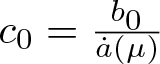 $c_{0}=\frac{b_{0}}{\dot{a}(\mu)}$ is some complex number, we can set
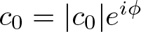 $c_{0}=|c_{0}|e^{i\phi}$
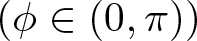 $(\phi\in(0,\pi))$. The linear equation system shown in formula (Equation 2.58) can be simplified as
 \begin{align}
\begin{split}
\tilde{N}_{1}(-\mu_{0})=&1+\frac{c_{0}e^{-2it\theta(\mu_{0})}}{-\mu_{0}-\mu_{0}}\tilde{N}_{1}(-\mu_{0})+
\frac{c^{*}_{0}e^{2it\theta^{*}(\mu_{0})}}{-\mu_{0}+\mu^{*}_{0}}\tilde{N}_{1}(\mu^{*}_{0})+\\
&\frac{-\frac{c_{0}}{\mu^{2}_{0}}e^{-2it\theta(\mu_{0})}}{-\mu_{0}+\frac{1}{\mu_{0}}}\tilde{N}_{1}(\frac{1}{\mu_{0}})+
\frac{-\frac{c^{*}_{0}}{\mu^{*2}_{0}}e^{2it\theta^{*}(\mu_{0})}}{-\mu_{0}-\frac{1}{\mu^{*}_{0}}}\tilde{N}_{1}(-\frac{1}{\mu^{*}_{0}}),
\end{split}
\end{align}
 \begin{align}
\begin{split}
\tilde{N}_{1}(\mu^{*}_{0})=&1+\frac{c_{0}e^{-2it\theta(\mu_{0})}}{\mu^{*}_{0}-\mu_{0}}\tilde{N}_{1}(-\mu_{0})+
\frac{c^{*}_{0}e^{2it\theta^{*}(\mu_{0})}}{\mu^{*}_{0}+\mu^{*}_{0}}\tilde{N}_{1}(\mu^{*}_{0})+\\
&\frac{-\frac{c_{0}}{\mu^{2}_{0}}e^{-2it\theta(\mu_{0})}}{\mu^{*}_{0}+\frac{1}{\mu_{0}}}\tilde{N}_{1}(\frac{1}{\mu_{0}})+
\frac{-\frac{c^{*}_{0}}{\mu^{*2}_{0}}e^{2it\theta^{*}(\mu_{0})}}{\mu^{*}_{0}-\frac{1}{\mu^{*}_{0}}}\tilde{N}_{1}(-\frac{1}{\mu^{*}_{0}}),
\end{split}
\end{align}
 \begin{align}
\begin{split}
\tilde{N}_{1}(\frac{1}{\mu_{0}})=&1+\frac{c_{0}e^{-2it\theta(\mu_{0})}}{\frac{1}{\mu_{0}}-\mu_{0}}\tilde{N}_{1}(-\mu_{0})+
\frac{c^{*}_{0}e^{2it\theta^{*}(\mu_{0})}}{\frac{1}{\mu_{0}}+\mu^{*}_{0}}\tilde{N}_{1}(\mu^{*}_{0})+\\
&\frac{-\frac{c_{0}}{\mu^{2}_{0}}e^{-2it\theta(\mu_{0})}}{\frac{1}{\mu_{0}}+\frac{1}{\mu_{0}}}\tilde{N}_{1}(\frac{1}{\mu_{0}})+
\frac{-\frac{c^{*}_{0}}{\mu^{*2}_{0}}e^{2it\theta^{*}(\mu_{0})}}{\frac{1}{\mu_{0}}-\frac{1}{\mu^{*}_{0}}}\tilde{N}_{1}(-\frac{1}{\mu^{*}_{0}}),
\end{split}
\end{align}
 \begin{align}
\begin{split}
\tilde{N}_{1}(-\frac{1}{\mu^{*}_{0}})=&1+\frac{c_{0}e^{-2it\theta(\mu_{0})}}{-\frac{1}{\mu^{*}_{0}}-\mu_{0}}\tilde{N}_{1}(-\mu_{0})+
\frac{c^{*}_{0}e^{2it\theta^{*}(\mu_{0})}}{-\frac{1}{\mu^{*}_{0}}+\mu^{*}_{0}}\tilde{N}_{1}(\mu^{*}_{0})+\\
&\frac{-\frac{c_{0}}{\mu^{2}_{0}}e^{-2it\theta(\mu_{0})}}{-\frac{1}{\mu^{*}_{0}}+\frac{1}{\mu_{0}}}\tilde{N}_{1}(\frac{1}{\mu_{0}})+
\frac{-\frac{c^{*}_{0}}{\mu^{*2}_{0}}e^{2it\theta^{*}(\mu_{0})}}{-\frac{1}{\mu^{*}_{0}}-\frac{1}{\mu^{*}_{0}}}\tilde{N}_{1}(-\frac{1}{\mu^{*}_{0}}).
\end{split}
\end{align}
After solving this linear system, inputting the results into formula (Equation 2.70), we can obtain the solution of 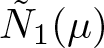 $\tilde{N}_{1}(\mu)$, then substituting it into the following formula
 \begin{align}
u(x,t)=-\left(
\frac{\tilde{N}^{\prime}_{1}(i)}{\tilde{N}_{1}(i)}+
\frac{\tilde{N}^{\prime}_{1}(-i)}{\tilde{N}_{1}(-i)}
\right),
\end{align}
where
 \begin{align}
x(y,t)=
y-\ln\left(\frac{\tilde{N}_{1}(-i)}{\tilde{N}_{1}(i)}\right),
\end{align}
we can obtain the solution of the cCH equation.
Next, we discuss the solution when scattering data  $a(\mu)$ has only two zero points through two examples, where the discrete spectrum has four points.
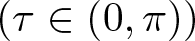
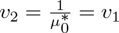
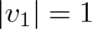
Case 1: Supposing  $v_{1}=\mu_{0}=e^{i\tau}\in\mathbb{C}^{+}$
 $(\tau\in(0,\pi))$,
 $v_{2}=\frac{1}{\mu^{*}_{0}}=v_{1}$. Then
 $|v_{1}|=1$, and we further assume that
 $\mu_{0}=r_{1}+ir_{2}$. It can be obtained that
 $\theta(e^{i\tau})=\theta(-e^{-i\tau})$. Next we define
 $\chi_{1}\triangleq\theta(e^{i\tau})=-\frac{i\sin\tau y}{2t}+\frac{i\sin\tau}{\cos^{2}\tau}$, hence
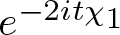 $e^{-2it\chi_{1}}$ is a real number about variables y and t. Thus algebraic system (Equation 2.70)–(Equation 2.74) have the following forms
 \begin{align}
\tilde{N}_{1}(\mu)=1+\frac{|c_{0}|e^{i\phi}e^{\chi_{1}}}{\mu-e^{i\tau}}\tilde{N}_{1}(-e^{i\tau})+
\frac{|c_{0}|e^{-i\phi}e^{\chi_{1}}}{\mu+e^{-i\tau}}\tilde{N}_{1}(e^{-i\tau}),
\end{align}
 \begin{align}
\begin{split}
\tilde{N}_{1}(-e^{i\tau})=&1+\frac{|c_{0}|e^{i\phi}e^{\chi_{1}}}{-2e^{i\tau}}\tilde{N}_{1}(-e^{i\tau})+
\frac{|c_{0}|e^{-i\phi}e^{\chi_{1}}}{e^{-i\tau}-e^{i\tau}}\tilde{N}_{1}(e^{-i\tau}),\\
\tilde{N}_{1}(e^{-i\tau})=&1+\frac{|c_{0}|e^{i\phi}e^{\chi_{1}}}{e^{-i\tau}-e^{i\tau}}\tilde{N}_{1}(-e^{i\tau})+
\frac{|c_{0}|e^{-i\phi}e^{\chi_{1}}}{2e^{-i\tau}}\tilde{N}_{1}(e^{-i\tau}),
\end{split}
\end{align}
then we have the solutions
 \begin{align}
\begin{split}
\tilde{N}_{1}(-e^{i\tau})=&\frac{1}{H_{1}}(1-\frac{r_{1}}{2ir_{2}}|c_{0}|e^{\chi_{1}-i\phi+i\tau}),\\
\tilde{N}_{1}(e^{-i\tau})=&\frac{1}{H_{1}}(1-\frac{r_{1}}{2ir_{2}}|c_{0}|e^{\chi_{1}+i\phi-i\tau}),
\end{split}
\end{align}
where
 \begin{align}
H_{1}=1+\frac{r^{2}_{1}}{4r^{2}_{2}}|c_{0}|e^{2\chi_{1}}+i|c_{0}|e^{\chi_{1}}\sin(\phi-\tau),
\end{align}
then we have
 \begin{align}
\begin{split}
\tilde{N}_{1}(\mu)=1+\frac{1}{H_{1}}\left(\frac{|c_{0}|e^{\phi+\chi_{1}}-
\frac{r_{1}|c_{0}|^{2}e^{2\chi_{1}+\phi}}{2ir_{2}e^{-i(\tau-\phi)}}}{\mu-e^{i\tau}}+
\frac{|c_{0}|e^{\chi_{1}-\phi}-\frac{r_{1}|c_{0}|^{2}e^{2\chi_{1}-\phi}}{2ir_{2}e^{i\tau}}}{\mu+e^{i(\tau-\phi)}}\right),
\end{split}
\end{align}
after assuming the parameter values are 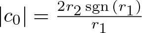 $|c_{0}|=\frac{2r_{2}\,\mathrm{sgn}\,(r_{1})}{r_{1}}$ and
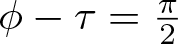 $\phi-\tau=\frac{\pi}{2}$, the expression of solution can be obtained as follows
 \begin{align}
u(x,t)=-\frac{4r_{2}}{r^{3}_{1}}\,\mathrm{sgn}\,(r_{1})\frac{\cosh(\chi_{1})}{cosh(2\chi_{1})+\frac{1+r^{2}_{2}}{r^{2}_{1}}},
\end{align}
with
 \begin{align}
x=x(y,t)=y-\ln\left(\frac{1+\frac{1+r_{2}}{1-r_{2}}e^{2\chi_{1}}}{1+\frac{1-r_{2}}{1+r_{2}}e^{2\chi_{1}}}\right).
\end{align}
Remark 2.8. By comparing with the soliton solution of cCH equation obtained in reference [Reference Matsuno31], it can be seen that the solution constructed by the RH method is exactly the same as the solution obtained by Hirota’s bilinear method after special parameter selection. Both of the above methods are used to study the construction of soliton solution for cCH equation under ZBCs. The difference is that [Reference Matsuno31] constructs multiple soliton solutions, while our article constructs arbitrary-order pole solutions. Similarly, when the orders of the zero points degenerate to one, the expressions of solutions obtained in these two articles are the same for multiple zero points case.
Remark 2.9. According to the detailed analysis of literature [Reference Matsuno31], it can be seen that when the parameters take different values, we can obtain smooth soliton solutions and symmetric singular soliton solutions. When the selected zero point µ 0 is complex and its modulus is not equal to zero, the breather solutions can be obtained.
From expression (Equation 2.83), it can be seen that when  $x\rightarrow\pm\infty$, there exists
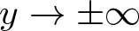 $y\rightarrow\pm\infty$. The solution (Equation 2.82) indicates that
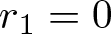 $r_{1}=0$
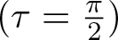 $(\tau=\frac{\pi}{2})$ is a singularity point and
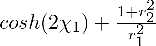 $cosh(2\chi_{1})+\frac{1+r^{2}_{2}}{r^{2}_{1}}$ has no zero point; otherwise, the following relationship will presence
 \begin{align}
r^{2}_{1}(e^{-2yr_{2}+\frac{2tr_{2}}{r^{2}_{1}}}+e^{2yr_{2}-\frac{2tr_{2}}{r^{2}_{1}}})=-2(1+r^{2}_{2}),
\end{align}
since the point 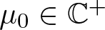 $\mu_{0}\in\mathbb{C}^{+}$, the right-hand side of the equation is always negative and the left-hand side is always positive, which leads to a contradiction. According to our analysis of constructing the RH problem, the points
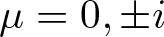 $\mu=0,\pm i$ are singularities which corresponding to the obtained solution. There
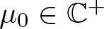 $\mu_{0}\in\mathbb{C}^{+}$ and it has only one singularity point
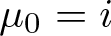 $\mu_{0}=i$.
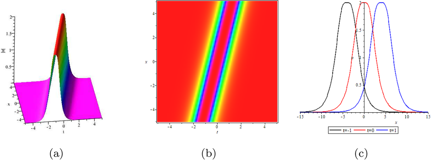
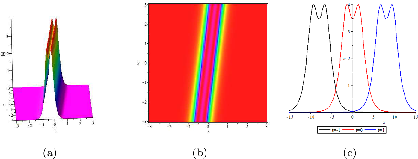
To demonstrate the characteristics of solitons, we present wave propagations including images of local structure, density, and intensity distribution in figures 2–4 after selecting different parameters. It can be seen that the single smooth soliton solutions are obtained at these values. Specifically, figure 2(a) shows a Hump soliton solution. figure 3(a) is a critical situation where the soliton exhibits a top horizontal characteristic. Finally, figure 4(a) shows the M-shape soliton solution. From these figures, it can be seen that as the values of τ increasing, the peak of the soliton first appears in a horizontal state and then sinks inward.
(a)–(c) describe the local structure, density, and intensity profiles with different times of one-soliton solution  $|u|$. Parameters
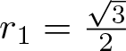 $r_{1}=\frac{\sqrt{3}}{2}$,
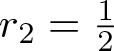 $r_{2}=\frac{1}{2}$,
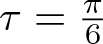 $\tau=\frac{\pi}{6}$.
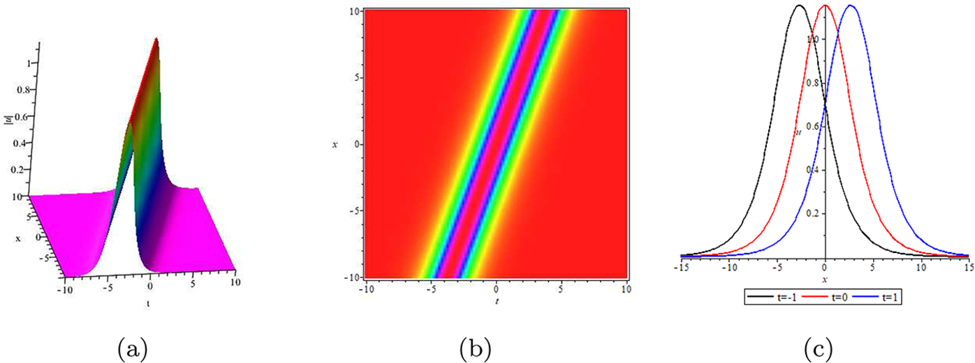
Figure 2 Long description
Three panels labeled (a), (b) and (c), each representing a different view of a one-soliton solution. Panel (a) is a 3D surface plot. The x-axis is labeled x, representing the spatial coordinate and ranges from approximately minus 10 to 10. The t-axis, representing time, ranges from approximately minus 5 to 5. The vertical z-axis represents the amplitude of the soliton field. The surface shows a single smooth localized peak rising sharply from a flat base, with the peak centered near x equals 0 and t equals 0. The peak amplitude reaches a maximum value visible at the apex of the surface and the surface slopes symmetrically downward in all directions from this central maximum. Panel (b) is a 2D contour density plot. The x-axis is labeled x and ranges from approximately minus 10 to 10. The y-axis is labeled t and ranges from approximately minus 5 to 5. The density plot shows a diagonal band running from the lower-left region to the upper-right region of the plot area, indicating that the soliton peak travels linearly across the spatial domain as time progresses. The band contains a sequence of contour regions reflecting high amplitude at the center and lower amplitude at the outer edges. Panel (c) is a line plot showing intensity profiles. The x-axis is labeled x and ranges from approximately minus 10 to 10. The y-axis represents amplitude or intensity magnitude. Three curves are plotted, each corresponding to a distinct parameter case as identified in the legend. The first curve, drawn with a solid line, shows the narrowest and tallest peak, centered near x equals 0, with the highest amplitude among the three curves. The second curve, drawn with a dashed line, shows a moderately wide peak of intermediate height, also centered near x equals 0. The third curve, drawn with a dash-dot line, shows the broadest and shortest peak among the three, centered near x equals 0. All three curves are symmetric about x equals 0 and each decays to near zero amplitude at the outer edges of the x range.
(a)–(c) describe the local structure, density, and intensity profiles with different times of one-soliton solution  $|u|$. Parameters
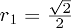 $r_{1}=\frac{\sqrt{2}}{2}$,
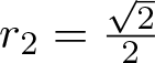 $r_{2}=\frac{\sqrt{2}}{2}$,
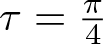 $\tau=\frac{\pi}{4}$.
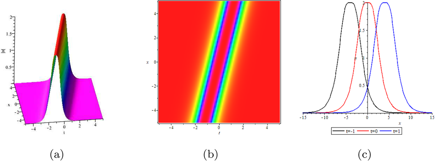
Figure 3 Long description
Three panels labeled (a), (b) and (c) present the local structure, density and intensity profiles of a one-soliton solution under different parameter conditions. Panel (a) is a three-dimensional surface plot. The horizontal axes are labeled x and t and the vertical axis represents the amplitude or intensity of the soliton solution. The surface shows a single smooth peak rising sharply from a near-flat base. The peak is located approximately at x equals 0 and t equals 0, reaching a maximum height of approximately 1.5 units on the vertical axis. The surface slopes symmetrically away from the peak in all directions, forming a bell-shaped mound. The base of the surface extends from approximately negative 4 to positive 4 along the x-axis and from negative 4 to positive 4 along the t-axis. Panel (b) is a two-dimensional density or intensity map. The horizontal axis is labeled x and the vertical axis is labeled t. Both axes appear to range from approximately negative 4 to positive 4. A narrow high-intensity band runs diagonally across the map from the lower-left region toward the upper-right region, indicating the trajectory of the soliton across the x-t plane. The surrounding region shows uniformly low intensity. The high-intensity band is narrow and well-defined, with the peak intensity concentrated along a central ridge. A colorbar is present alongside the plot, with lower values at one end and higher values at the other end, corresponding to the intensity range across the map. Panel (c) contains three overlapping line profiles plotted on the same axes. The horizontal axis represents x, ranging from approximately negative 10 to positive 10. The vertical axis represents intensity, ranging from 0 to approximately 1.5. Three curves are shown, each corresponding to a different parameter value as indicated in the legend, which lists three entries distinguished by different line styles. The first curve is centered near x equals negative 2, reaching a peak of approximately 1.4. The second curve is centered near x equals 0, reaching a peak of approximately 1.4. The third curve is centered near x equals positive 2, reaching a peak of approximately 1.4. All three curves have similar heights and widths, but their horizontal positions differ, indicating a lateral shift in the soliton position as the parameter changes. Each curve has a symmetric bell shape with a full width at approximately half maximum of roughly 2 units.
(a)–(c) describe the local structure, density, and intensity profiles with different times of one-soliton solution  $|u|$. Parameters
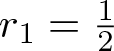 $r_{1}=\frac{1}{2}$,
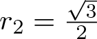 $r_{2}=\frac{\sqrt{3}}{2}$,
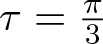 $\tau=\frac{\pi}{3}$.

Figure 4 Long description
Plot (a) is a three-dimensional surface plot. The horizontal axes represent spatial coordinates and the vertical axis represents amplitude. The surface shows a single narrow peak rising sharply from a flat background near zero. The peak is smooth and symmetric, with the surrounding region remaining uniformly low. Plot (b) is a two-dimensional density or intensity map. Both axes represent spatial coordinates. A single diagonal high-intensity stripe runs across the plot from one corner toward the opposite side. The surrounding area shows uniformly low intensity. The stripe is narrow and well-defined. Plot (c) shows line graphs of intensity profiles. The horizontal axis represents spatial position and the vertical axis represents intensity. Three curves are plotted, each corresponding to a different time value as indicated by the legend. Each curve shows a single peak. The three peaks are centered at different positions along the horizontal axis, indicating a shift in peak location across the three time values. The peaks appear similar in height and width. The legend identifies three separate entries corresponding to the three curves shown.
Case 2: Supposing  $v_{1}=\mu_{0}=ir\in i\mathbb{R}$,
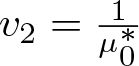 $v_{2}=\frac{1}{\mu^{*}_{0}}$. It can be obtained that
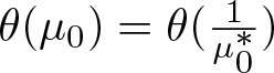 $\theta(\mu_{0})=\theta(\frac{1}{\mu^{*}_{0}})$. Next we define
 $\chi_{2}\triangleq\theta(\mu_{0})=-\frac{i}{4}\frac{r^{2}+1}{r}\left(\frac{y}{t}+\frac{8r^{2}}{(r^{2}-1)^{2}}\right)$, hence
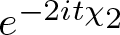 $e^{-2it\chi_{2}}$ is a real number about variables y and t. Thus algebraic system (Equation 2.70)–(Equation 2.74) have the following forms
 \begin{align}
\tilde{N}_{1}(\mu)=1+\frac{|c_{0}|e^{i\phi}e^{\chi_{2}}}{\mu-ir}\tilde{N}_{1}(-ir)+
\frac{\frac{|c_{0}|}{r^{2}}e^{-i\phi}e^{\chi_{2}}}{\mu+\frac{1}{ir}}\tilde{N}_{1}(\frac{1}{ir}),
\end{align}
 \begin{align}
\begin{split}
\tilde{N}_{1}(-ir)=&1+\frac{|c_{0}|e^{i\phi}e^{\chi_{2}}}{-2ir}\tilde{N}_{1}(-ir)+
\frac{\frac{|c_{0}|}{r^{2}}e^{-i\phi}e^{\chi_{2}}}{-ir+\frac{1}{ir}}\tilde{N}_{1}(\frac{1}{ir}),\\
\tilde{N}_{1}(\frac{1}{ir})=&1+\frac{|c_{0}|e^{i\phi}e^{\chi_{2}}}{\frac{1}{ir}-ir}\tilde{N}_{1}(-ir)+
\frac{\frac{|c_{0}|}{r^{2}}e^{-i\phi}e^{\chi_{2}}}{\frac{2}{ir}}\tilde{N}_{1}(\frac{1}{ir}),
\end{split}
\end{align}
the solutions are
 \begin{align}
\begin{split}
\tilde{N}_{1}(-ir)=&\frac{1}{H_{2}}(1-\frac{1-r^2}{2ir(1+r^2)}|c_{0}|e^{\chi_{2}+\phi}),\\
\tilde{N}_{1}(\frac{1}{ir})=&\frac{1}{H_{2}}(1+\frac{1-r^2}{2ir(1+r^2)}|c_{0}|e^{\chi_{2}+\phi}),
\end{split}
\end{align}
with
 \begin{align}
H_{2}=1-\frac{(r^{2}-1)^{2}}{4r^{2}(r^{2}+1)^{2}}|c_{0}|^{2}e^{2\chi_{2}}-\frac{i|c_{0}|e^{\chi_{2}+\phi}}{r}.
\end{align}
Substitute formula (Equation 2.87) into (Equation 2.85) and take an appropriate value for c 0 to calculate the solution as follows
 \begin{align}
u(x,t)=\frac{16r^2(1+r^2)}{(1-r^2)^3}\frac{\sinh(\chi_{2})}{cosh(2\chi_{2})+\frac{(1+r^{2})^2+4r^2}{(1-r^2)^2}},
\end{align}
with
 \begin{align}
x=x(y,t)=y-\ln\left(\frac{1+\frac{(1+r)^2}{(1-r)^2}e^{2\chi_{2}}}{1+\frac{(1-r)^2}{(1+r)^2}e^{2\chi_{2}}}\right).
\end{align}
The solution (Equation 2.89) indicates that r = 1 is a singularity point and  $cosh(2\chi_{2})+\frac{(1+r^{2})^2+4r^2}{(1-r^2)^2}$ has no zero point; otherwise, the following relationship will presence
 \begin{align}
(1-r^2)^2(e^{2\chi_{2}}+e^{-2\chi_{2}})=-2(1+r^2)^2-8r^4,
\end{align}
this is clearly impossible.
Remark 2.10. After comparison, when selecting appropriate parameters, the expression of solution (Equation 2.89) solved by RH approach is the same as the solution (3.9a) solved by Hirota’s bilinear method in reference [Reference Matsuno31]. Then the antisymmetric singular soliton can be obtained.
2.3.2. Two-order pole solution
For the N = 2 case, it corresponds to the solution with a two-order pole. The expression of 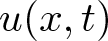 $u(x,t)$ defined in theorem 2.7.
Case 3: Assuming that  $v_{1}=\mu_{0}=e^{i\tau}$ be one two-order zero point of the scattering data
 $a(\mu)$, then
 $v_{2}=e^{i\tau}=v_{1}$ is also the two-order zero point of
 $a(\mu)$. The discrete spectrum is the set
 $\mathcal{Z}=\left\{e^{i\tau}, -e^{-i\tau}, e^{-i\tau}, -e^{i\tau}\right\}$. We choose some parameters to simulate the solution, then the different dynamic models can be obtained in Figures (5)–(6).
(a)–(c) describe the local structure, density, and intensity profiles with different times of the soliton solutions  $|u|$ with one two-order pole. Parameters
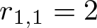 $r_{1,1}=2$,
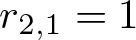
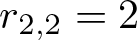
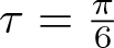
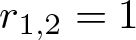 $r_{1,2}=1$,
 $r_{2,1}=1$,
 $r_{2,2}=2$,
 $\tau=\frac{\pi}{6}$.

Figure 5 Long description
(a) A 3D surface plot showing the local structure of soliton solutions over time. The axes are labeled x, t and z, representing spatial and temporal dimensions. A diagonal ridge indicates a significant feature in the data. (b) A heatmap displaying density profiles with axes labeled from negative 20 to positive 20. The color scale represents varying density levels, transitioning from red to blue. (c) A line graph illustrating intensity profiles with the horizontal axis from negative 20 to positive 20 and the vertical axis from 0 to 40. The legend shows different colored lines representing distinct intensity levels. Peaks and troughs indicate changes in intensity over time. Together, these graphs demonstrate the relationship between structure, density and intensity in soliton solutions, highlighting key features and transitions.
(a)–(c) describe the local structure, density, and intensity profiles with different times of the soliton solutions  $|u|$ with one two-order pole. Parameters
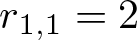 $r_{1,1}=2$,
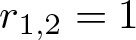 $r_{1,2}=1$,
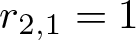 $r_{2,1}=1$,
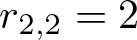 $r_{2,2}=2$,
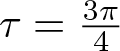 $\tau=\frac{3\pi}{4}$.

Figure 6 Long description
A) Three-dimensional surface plot representing the local structure profile of a soliton solution. The vertical axis represents amplitude or wave quantity and the two horizontal axes represent spatial and temporal coordinates. The surface forms a largely flat plane with a single sharp, narrow ridge running diagonally across it, indicating a localized elevation concentrated along one axis direction. The ridge rises steeply from the flat base and drops back sharply, consistent with a single soliton structure. Axis labels and numeric tick values are not legible at this resolution. B) Two-dimensional density plot representing the spatial and temporal evolution of the soliton solution. The horizontal axis represents one coordinate, spanning approximately minus 15 to 15 and the vertical axis represents the other coordinate, spanning approximately minus 10 to 10. The plot is divided into two broad regions separated by a narrow, sharply curved transition band running vertically near the left portion of the domain. A vertical color scale bar is included alongside the plot. The transition band is narrow and well-defined, indicating a steep gradient in the plotted quantity across that boundary. The two surrounding regions appear uniform in value, with the transition being the dominant feature. C) Two-dimensional intensity profile plot. The horizontal axis represents a spatial or temporal coordinate and the vertical axis represents intensity or magnitude of the soliton solution. Multiple overlaid traces are present, with at least three distinguishable curves. All traces remain near the zero baseline across most of the domain. Near one end of the horizontal axis, several narrow, tall peaks appear in close proximity. One peak is visibly taller than the others. The remaining peaks are smaller but still sharply defined. The peaks are clustered within a narrow region of the domain. A vertical reference line is also drawn near the peak cluster. The traces overlap closely in the flat baseline region and diverge only at the peak locations.
Setting 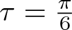 $\tau=\frac{\pi}{6}$ and
 $\left\{r_{1,1}=2, r_{1,2}=1, r_{2,1}=1, r_{2,2}=2\right\}$. On the basis of the construction process of single high-order pole solutions, the following relationships are calculated.
 \begin{align*}
\zeta_{1,0}=\zeta_{2,0}=e^{\frac{4t}{3}-\frac{y}{2}},\quad
\zeta_{1,1}=\zeta_{2,1}=\frac{-8i(40t-9y)e^{\frac{4t}{3}-\frac{y}{2}}(i\sqrt{3}-1)}
{(i\sqrt{3}+3)^3(\sqrt{3}+i)^2},
\end{align*}
 \begin{align*}
\vartheta_{1,1}=\vartheta_{1,3}=\frac{5\sqrt{3}e^{\frac{4t}{3}-\frac{y}{2}}}{9}
\left(\sqrt{3}\left(\frac{21+27y}{40}-\frac{3i}{2}-3t\right)+it-\frac{9i(y-1)}{40}+\frac{9}{10}\right),
\end{align*}
 \begin{align*}
\vartheta_{1,2}=\vartheta_{1,4}=-\frac{2880e^{\frac{4t}{3}-\frac{y}{2}}}{(i\sqrt{3}+3)^3(\sqrt{3}+i)^4}
\left(\sqrt{3}\left(\frac{6-y}{40}-\frac{i}{10}+\frac{t}{9}\right)+it-\frac{9i(y+1)}{40}-\frac{1}{2}\right),
\end{align*}
 \begin{align*}
\vartheta_{3,1}=\vartheta_{3,3}=\frac{10\sqrt{3}e^{\frac{4t}{3}-\frac{y}{2}}}{9}
\left(\sqrt{3}\left(\frac{21+27y}{40}-\frac{3i}{8}-3t\right)+it-\frac{9i(y-1)}{40}+\frac{9}{40}\right),
\end{align*}
 \begin{align*}
\vartheta_{3,2}=\vartheta_{3,4}=-\frac{5760e^{\frac{4t}{3}-\frac{y}{2}}}{(i\sqrt{3}+3)^3(\sqrt{3}+i)^4}
\left(\sqrt{3}\left(\frac{6-y}{40}-\frac{i}{40}+\frac{t}{9}\right)+it-\frac{9i(y+2)}{40}-\frac{1}{8}\right),
\end{align*}
 \begin{align*}
\vartheta_{2,1}=\vartheta_{2,3}=-\frac{e^{\frac{4t}{3}-\frac{y}{2}}(i\sqrt{3}-2)}{\sqrt{3}+i},\quad
\vartheta_{2,2}=\vartheta_{2,4}=-\frac{e^{\frac{4t}{3}-\frac{y}{2}}(2i\sqrt{3}+3)}{(\sqrt{3}+i)^{2}},
\end{align*}
 \begin{align*}
\vartheta_{4,1}=\vartheta_{4,3}=-\frac{e^{\frac{4t}{3}-\frac{y}{2}}(2i\sqrt{3}-4)}{\sqrt{3}+i},\quad
\vartheta_{4,2}=\vartheta_{4,4}=-\frac{e^{\frac{4t}{3}-\frac{y}{2}}(4i\sqrt{3}+6)}{(\sqrt{3}+i)^{2}},
\end{align*}
 \begin{align*}
\eta_{11}=-2e^{\frac{4t}{3}-\frac{y}{2}}-\frac{8ie^{\frac{4t}{3}-\frac{y}{2}}(1+i\sqrt{3})(40t-9y)}{(i\sqrt{3}-3)^3(i-\sqrt{3})^2},\quad
\eta_{12}=-e^{\frac{4t}{3}-\frac{y}{2}},
\end{align*}
 \begin{align*}
\eta_{21}=-e^{\frac{4t}{3}-\frac{y}{2}}-\frac{16ie^{\frac{4t}{3}-\frac{y}{2}}(1+i\sqrt{3})(40t-9y)}{(i\sqrt{3}-3)^3(i-\sqrt{3})^2},\quad
\eta_{22}=-2e^{\frac{4t}{3}-\frac{y}{2}}.
\end{align*}
Substitute the above results into the expression of solution (Equation 2.67) to obtain the two-order pole solution, and the propagation phenomenon of soliton is shown in figure 5. It can be seen that the energies of two waves for solution decrease after collision; thus, it is not an elastic collision that occurs. According to the previous analysis, the singularity of the solution is 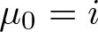 $\mu_{0}=i$.
Using a similar analysis, when the value is set to 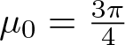 $\mu_{0}=\frac{3\pi}{4}$, the soliton dynamics behaviour shown in figure 6. figure 6(b) presents the density image of the wave propagation process, while figure 6(c) shows the intensity distribution at different times.
2.4. Multiple high-order pole solutions
Now the general circumstance that  $a(\mu)$ has N high-order zero points
 $\mu_{1},\mu_{2},\ldots,\mu_{N}$,
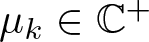 $\mu_{k}\in\mathbb{C}^{+}$ for
 $k=1,2,\ldots,N$ and the corresponding powers are
 $n_{1},n_{2},\ldots,n_{N}$, respectively. Assume that
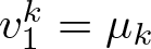 $v^{k}_{1}=\mu_{k}$ and
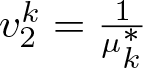 $v^{k}_{2}=\frac{1}{\mu^{*}_{k}}$. Similar to the case of one high-order pole, from the definition of
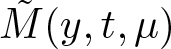 $\tilde{M}(y,t,\mu)$, it can be seen that
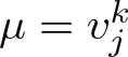 $\mu=v^{k}_{j}$ and
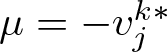 $\mu=-v^{k*}_{j}$
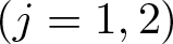 $(j=1,2)$ are nk-order pole points of
 $\tilde{M}_{11}$. Simultaneously,
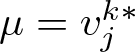 $\mu=v^{k*}_{j}$ and
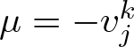 $\mu=-v^{k}_{j}$
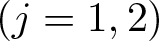 $(j=1,2)$ are nk-order pole points of
 $\tilde{M}_{12}$.
Under the assumption that 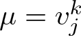 $\mu=v^{k}_{j}$
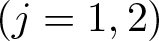 $(j=1,2)$ are nk-order zero points of
 $a(\mu)$ for
 $k=1,2,\ldots,N$, utilizing the Wronskian
 $a(\mu)=Wr(\breve{\phi}_{-1},\breve{\phi}_{+2})$, there exist complex constants
 $b^{k}_{j,s}$
 $(s=1,2,\cdots,n_N)$ satisfy the follows
 \begin{equation}
\frac{\partial^{m}[\tilde{\phi}_+(y,t,v^{k}_{j})]_{2}}{\partial\mu^{m}}=\sum^{m}_{l=0}\left(\begin{array}{c}
m \\
l
\end{array}\right)
b^{k}_{j,m-l+1}\frac{\partial^{l}[\tilde{\phi}_-(y,t,v^{k}_{j})]_{1}}{\partial\mu^{l}},
\end{equation}
and
 \begin{equation}
\frac{\partial^{m}[\tilde{\psi}_+(y,t,v^{k}_{j})]_{2}}{\partial\mu^{m}}=\sum^{m}_{l=0}\left(\begin{array}{c}
m \\
l
\end{array}\right)
b^{k}_{j,m-l+1}\frac{\partial^{l}[\tilde{\psi}_-(y,t,v^{k}_{j})]_{1}e^{2it\theta(v^{k}_{j})}}{\partial\mu^{l}},
\end{equation}
with  $m=0,1,\ldots,n_{N-1}$. Utilizing the parallel approach in above, we define the
 $n_k\times n_k$ matrices
 $\Theta^{j,p}_{kd}=[\Theta^{j,p}_{kd}]_{s,q}$ and
 $\tilde{\Theta}^{j,p}_{kd}=[\tilde{\Theta}^{j,p}_{kd}]_{s,q}$ for
 $s,q=1,2,\cdots,n_{k}$ and introduce the following notations for
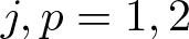 $j,p=1,2$
 \begin{align}
|\eta^{k}_{j}\rangle=(\eta^{k}_{j1},\cdots,\eta^{k}_{jn_{k}})^{T},\quad
\eta^{k}_{js}=-\sum_{l=s}^{n_{k}}r^{k*}_{j,l}\zeta^{k*}_{j,l-s}(y,t),
\end{align}
 \begin{align}
r^{k}_{j,l}=\lim_{\mu\rightarrow v^{k}_{j}}\frac{b^{k}_{j,l}}{(n_{k}-l)!}\frac{\partial^{n_{k}-l}}{\partial(\mu-v^{k}_{j})^{n_{k}-l}}
\frac{(\mu-v^{k}_{j})^{n_{k}}}{a(\mu)},
\end{align}
 \begin{align}
|\Gamma\rangle=(|\Gamma^{1}\rangle,\cdots,|\Gamma^{N}\rangle)^{T},\quad
|\Gamma^{k}\rangle=(|\eta^{k}_{1}\rangle,|\eta^{k}_{2}\rangle)^{T},
\end{align}
 \begin{align}
\begin{split}
\Theta^{j,p}_{kd}=\sum_{l=s}^{n_k}\sum_{m=0}^{l-s}
\left(
\begin{array}{c}
q+m-1\\
m \\
\end{array}
\right)
r^{k}_{j,l}\zeta^{k}_{j,l-s-m}\left\{\frac{(-1)^{m}}{(v^{k}_{j}-v^{k*}_{p})^{q+m}}
+\frac{(-1)^{m+q+1}}{(v^{k}_{j}+v^{k}_{p})^{q+m}}\right\},
\end{split}
\end{align}
 \begin{align}
\begin{split}
\tilde{\Theta}^{j,p}_{kd}=\sum_{l=s}^{n_k}\sum_{m=0}^{l-s}
\left(
\begin{array}{c}
q+m-1\\
m \\
\end{array}
\right)
r^{k*}_{j,l}\zeta^{k*}_{j,l-s-m}\left\{\frac{(-1)^{m}}
{(v^{k*}_{j}-v^{k}_{p})^{q+m}}
+\frac{(-1)^{m+q}}{(v^{k*}_{j}+v^{k*}_{p})^{q+m}}\right\},
\end{split}
\end{align}
 \begin{align}
\Theta=
\begin{pmatrix}
[\Theta^{j,p}_{11}] & \cdots & [\Theta^{j,p}_{1N}] \\
\vdots & \ddots & \vdots \\
[\Theta^{j,p}_{N1}] & \cdots & [\Theta^{j,p}_{NN}] \\
\end{pmatrix},\quad
\tilde{\Theta}=
\begin{pmatrix}
[\tilde{\Theta}^{j,p}_{11}] & \cdots & [\tilde{\Theta}^{j,p}_{1N}] \\
\vdots & \ddots & \vdots \\
[\tilde{\Theta}^{j,p}_{N1}] & \cdots & [\tilde{\Theta}^{j,p}_{NN}] \\
\end{pmatrix},
\end{align}
 \begin{align}
I_{\epsilon}=
\begin{pmatrix}
I_{\epsilon_{1}} & & \\
& \ddots & \\
& & I_{\epsilon_{N}} \\
\end{pmatrix},\quad
I_{\epsilon_{k}}=
\begin{pmatrix}
I & \\
& I \\
\end{pmatrix}_{2n_{k}\times2n_{k}} k=1,\cdots,N,
\end{align}
 \begin{equation}
\begin{split}
&\langle Y(\mu)|=(\langle Y^{1}_{1}(\mu)|,\langle Y^{1}_{2}(\mu)|,\cdots,\langle Y^{N}_{1}(\mu)|,\langle Y^{N}_{2}(\mu)|),\\
&\langle\tilde{Y}(\mu)|
=(\langle\tilde{Y}^{1}_{1}(\mu)|,\langle\tilde{Y}^{1}_{2}(\mu)|,\cdots,
\langle\tilde{Y}^{N}_{1}(\mu)|,\langle\tilde{Y}^{N}_{2}(\mu)|),\\
&\langle Y^{\prime}(\mu)|=
(\langle Y^{1\prime}_{1}(\mu)|,\langle Y^{1\prime}_{2}(\mu)|,\cdots,
\langle Y^{N\prime}_{1}(\mu)|,\langle Y^{N\prime}_{2}(\mu)|),\\
&\langle\tilde{Y}^{\prime}(\mu)|
=(\langle\tilde{Y}^{1\prime}_{1}(\mu)|,\langle\tilde{Y}^{1\prime}_{2}(\mu)|,\cdots,
\langle\tilde{Y}^{N\prime}_{1}(\mu)|,\langle\tilde{Y}^{N\prime}_{2}(\mu)|),
\end{split}
\end{equation}
 \begin{align*}
&\langle Y^{k}_{j}(\mu)|=(Y^{k}_{j1},\cdots,Y^{k}_{jn_k}),\quad
Y^{k}_{js}=\frac{1}{(\mu-v^{k}_{j})^{s}}+\frac{(-1)^{s}}{(\mu+v^{k*}_{j})^{s}},\\
&\langle\tilde{Y}^{k}_{j}(\mu)|=(\tilde{Y}^{k}_{j1},\cdots,\tilde{Y}^{k}_{jn_k}),\quad
\tilde{Y}^{k}_{js}=\frac{1}{(\mu-v^{k*}_{j})^{s}}+\frac{(-1)^{s+1}}{(\mu+v^{k}_{j})^{s}},\\
&\langle Y^{k\prime}_{j}(\mu)|=(Y^{k\prime}_{j1},\cdots,Y^{k\prime}_{jn_k}),\quad
Y^{k\prime}_{js}=\frac{-s}{(\mu-v^{k}_{j})^{s+1}}+\frac{s(-1)^{s+1}}{(\mu+v^{k*}_{j})^{s+1}},\\
&\langle\tilde{Y}^{k\prime}_{j}(\mu)|=(\tilde{Y}^{k\prime}_{j1},\cdots,\tilde{Y}^{k\prime}_{jn_k}),\quad
\tilde{Y}^{k\prime}_{js}=\frac{-s}{(\mu-v^{k*}_{j})^{s+1}}+\frac{s(-1)^{s}}{(\mu+v^{k}_{j})^{s+1}}.
\end{align*}
Similar to the theorem 2.7, we give the solution of cCH equation with multiple high-order poles as follows.
Theorem 2.11
The solution of cCH equation with multiple high-order poles under the ZBCs can be obtained as follows
 \begin{align}
u(x,t)=-\left(
\frac{\tilde{M}^{\prime}_{11}(i)+\tilde{M}^{\prime}_{21}(i)}{\tilde{M}_{11}(i)+\tilde{M}_{21}(i)}+
\frac{\tilde{M}^{\prime}_{12}(i)+\tilde{M}^{\prime}_{22}(i)}{\tilde{M}_{12}(i)+\tilde{M}_{22}(i)}
\right),
\end{align}
with
 \begin{align*}
&\tilde{M}_{11}(i)=\frac{\det(I_{\epsilon}+\Theta\tilde{\Theta}+|\Gamma\rangle\langle Y(i)|\Theta)}
{\det(I_{\epsilon}+\Theta\tilde{\Theta})},\\
&\tilde{M}_{21}(i)=-\frac{\det(I_{\epsilon}+\Theta^{*}\tilde{\Theta}^{*}+|\Gamma^{*}\rangle\langle\tilde{Y}^{*}(-i)|)}
{\det(I_{\epsilon}+\Theta^{*}\tilde{\Theta}^{*})}+1,\\
&\tilde{M}_{12}(i)=\frac{\det(I_{\epsilon}+\tilde{\Theta}\Theta+|\Gamma\rangle\langle\tilde{Y}(i)|)}
{\det(I_{\epsilon}+\tilde{\Theta}\Theta)}-1,\\
&\tilde{M}_{22}(i)=\frac{\det(I_{\epsilon}+\tilde{\Theta}^{*}\Theta^{*}+|\Gamma^{*}\rangle\langle Y^{*}(-i)|\Theta^{*})}
{\det(I_{\epsilon}+\tilde{\Theta}^{*}\Theta^{*})},\\
&\tilde{M}^{\prime}_{11}(i)=\frac{\det(I_{\epsilon}+\Theta\tilde{\Theta}+|\Gamma\rangle\langle Y^{\prime}(i)|\Theta)}
{\det(I_{\epsilon}+\Theta\tilde{\Theta})}-1,\\
&\tilde{M}^{\prime}_{21}(i)=-\frac{\det(I_{\epsilon}+\Theta^{*}\tilde{\Theta}^{*}+|\Gamma^{*}\rangle\langle\tilde{Y}^{\prime *}(-i)|)}
{\det(I_{\epsilon}+\Theta^{*}\tilde{\Theta}^{*})}+1,\\
&\tilde{M}^{\prime}_{12}(i)=\frac{\det(I_{\epsilon}+\tilde{\Theta}\Theta+|\Gamma\rangle\langle\tilde{Y}^{\prime}(i)|)}
{\det(I_{\epsilon}+\tilde{\Theta}\Theta)}-1,\\
&\tilde{M}^{\prime}_{22}(i)=\frac{\det(I_{\epsilon}+\tilde{\Theta}^{*}\Theta^{*}+|\Gamma^{*}\rangle\langle Y^{\prime *}(-i)|\Theta^{*})}
{\det(I_{\epsilon}+\tilde{\Theta}^{*}\Theta^{*})}-1,
\end{align*}
and 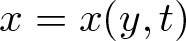 $x=x(y,t)$ can be obtained by (Equation 2.41), the elements
 $|\Gamma\rangle$, Iϵ, Θ,
 $\tilde{\Theta}$,
 $\langle Y(i)|$,
 $\langle\tilde{Y}(i)|$,
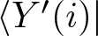 $\langle Y^{\prime}(i)|$ and
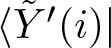 $\langle \tilde{Y}^{\prime}(i)|$ are defined in (Equation 2.96), (Equation 2.99), (Equation 2.100), and (Equation 2.101).
3. RH problem and high-order pole under NZBCs
3.1. Spectral analysis
After doing the transformations  $u(x,t)=\hat{u}(x-t,t)+1$,
 $\hat{m}=\hat{u}-\hat{u}_{xx}+1$ and
 $\hat{R}=\hat{u}^{2}-\hat{u}^{2}_{x}+2\hat{u}$, the Lax pair (Equation 2.1) admits the forms
 \begin{align}
\hat{\phi}_{x}=\hat{U}\hat{\phi},\quad \hat{\phi}_{t}=\hat{V}\hat{\phi},
\end{align}
 \begin{align}
\hat{U}=\left(\begin{array}{cc}
-\frac{Q}{2} & \frac{\lambda \hat{m}}{2} \\
-\frac{\lambda \hat{m}}{2} & \frac{Q}{2}
\end{array}\right),
\hat{V}=\left(\begin{array}{cc}
\frac{Q}{\lambda^{2}}+\frac{Q\hat{R}}{2} & -\frac{\hat{u}-Q\hat{u}_x+1}{\lambda}-\frac{\lambda \hat{R}\hat{m}}{2} \\
\frac{\hat{u}+Q\hat{u}_x+1}{\lambda}+\frac{\lambda \hat{R}\hat{m}}{2} & -\frac{Q}{\lambda^{2}}-\frac{Q\hat{R}}{2}
\end{array}\right).
\end{align}
Using the similar approach with ZBCs, we have the gauge transformation
 \begin{align}
\hat{\psi}=F^{-1}\hat{\phi} e^{\hat{J}},
\end{align}
with
 \begin{align*}
F=\left(\begin{array}{cc}
1 & \frac{\lambda}{\sqrt{Q^{2}-\lambda^{2}}+Q} \\
\frac{\lambda}{\sqrt{Q^{2}-\lambda^{2}}+Q} & 1
\end{array}\right),
\end{align*}
where we define 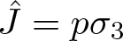 $\hat{J}=p\sigma_{3}$.
 $\hat{\psi}$ satisfies the asymptotic conditions
 \begin{align*}
\hat{\psi}(x,t,\lambda)\sim I,\quad x\rightarrow\pm\infty.
\end{align*}
The parameter 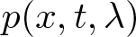 $p(x,t,\lambda)$ is defined as follows
 \begin{align}
p=\frac{\sqrt{1-2\lambda^{2}}}{2}\left(x-\int_{x}^{+\infty}(\hat{m}(\xi,t)-1)d\xi
-\frac{2}{\lambda^{2}}t\right).
\end{align}
Equation (Equation 1.3) admits the following form Lax pair
 \begin{align}
&\hat{\psi}_x+[\hat{J}_x,\hat{\psi}]=\hat{X}\hat{\psi},
\end{align}
 \begin{align}
&\hat{\psi}_t+[\hat{J}_t,\hat{\psi}]=\hat{T}\hat{\psi},
\end{align}
with
 \begin{align*}
\hat{X}=\frac{\lambda(\hat{m}-1)Q}{2\sqrt{1-2\lambda^{2}}}
\left(\begin{array}{cc}
0 & 1 \\
-1 & 0
\end{array}\right)+
\frac{(\hat{m}-1)Q^{2}}{2\sqrt{1-2\lambda^{2}}}
\left(\begin{array}{cc}
1 & 0 \\
0 & -1
\end{array}\right),
\end{align*}
 \begin{align*}
\hat{T}=&\frac{1}{2\sqrt{1-2\lambda^{2}}}\left(\lambda\hat{R}(\hat{m}-1)+\frac{2\hat{u}}{\lambda}\right) Q\left(\begin{array}{cc}
0 & -1 \\
1 & 0
\end{array}\right)+
\frac{\hat{u}_{x}Q}{\lambda}
\left(\begin{array}{cc}
0 & 1 \\
1 & 0
\end{array}\right) \\
&-\frac{1}{\sqrt{1-2\lambda^{2}}}\left(\hat{u}+\frac{1}{2}((\hat{m}-1)\hat{R}+2\hat{u})Q^{2}-\lambda^{2}\hat{u}\right)\sigma_{3},
\end{align*}
where 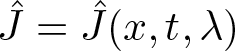 $\hat{J}=\hat{J}(x,t,\lambda)$,
 $\hat{X}=\hat{X}(x,t,\lambda)$,
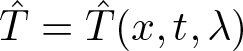 $\hat{T}=\hat{T}(x,t,\lambda)$ are
 $2\times2$ matrices.
A new spectral parameter k satisfied  $2\lambda^{2}=4k^{2}+1$ is introduced, and to avoid multi-value problem, we define
 \begin{equation}
\lambda=-\frac{1}{2\sqrt{2}}\left(\mu+\frac{1}{\mu}\right),\quad
k=\frac{1}{4}\left(\mu-\frac{1}{\mu}\right),
\end{equation}
then we have
 \begin{equation}
p=-\frac{i(\mu^{2}-1)}{4\mu}\left(\int_{x}^{+\infty}(\hat{m}(\xi,t)-1)d\xi-x+
\frac{16\mu^{2}}{(\mu^{2}+1)^{2}}t\right),
\end{equation}
and
 \begin{align*}
\hat{X}(x,t,\mu)&=\frac{i((\mu^{2}+1)^{2}-8\mu^{2})(\hat{m}-1)}{8\mu(\mu^{2}-1)}\sigma_{3}\\
&+\frac{i(\mu^{2}+1)\sqrt{8\mu^{2}-(\mu^{2}+1)^{2}}(\hat{m}-1)}{8|\mu|(\mu^{2}-1)}
\left(\begin{array}{cc}
0 & 1 \\
-1 & 0
\end{array}\right),
\end{align*}
the two Jost solutions of (Equation 3.5a) with the parameter µ are completely determined by Volterra integrable equations
 \begin{align}
\hat{\psi}_{\pm}(x,t,\mu)=I+\int_{\pm\infty}^{x}e^{\frac{i(\mu^{2}-1)}{4\mu}\int_{x}^{\xi}\hat{m}(\tau,t)d\tau\hat{\sigma}_{3}}
\left[\hat{X}(\xi,t,\mu)\hat{\psi}_{\pm}(\xi,t,\mu)\right]d\xi.
\end{align}
The Jost eigenfunctions 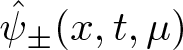 $\hat{\psi}_{\pm}(x,t,\mu)$ have the analytic properties, symmetry properties, and asymptotic properties shown in the following three propositions.
Proposition 3.1. Providing that  $u_{0}(x)-1\in L^{1}(\mathbb{R}^{\pm})$, the Jost eigenfunctions
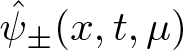 $\hat{\psi}_{\pm}(x,t,\mu)$ have the following analytic properties.
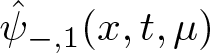 $\hat{\psi}_{-,1}(x,t,\mu)$ and
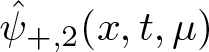 $\hat{\psi}_{+,2}(x,t,\mu)$ are analytic in
 $\mathbb{C}^{+}$ and continuously extended to
 $\mathbb{C}^{+}\cup\mathbb{R}$ except the points
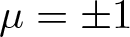 $\mu=\pm 1$,
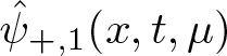 $\hat{\psi}_{+,1}(x,t,\mu)$ and
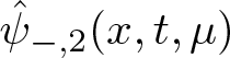 $\hat{\psi}_{-,2}(x,t,\mu)$ are analytic in
 $\mathbb{C}^{-}$ and continuously extended to
 $\mathbb{C}^{-}\cup\mathbb{R}$ except the points
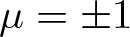 $\mu=\pm 1$, there
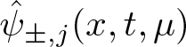 $\hat{\psi}_{\pm,j}(x,t,\mu)$ (
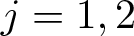 $j=1,2$) represent the j-th column of
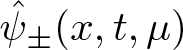 $\hat{\psi}_{\pm}(x,t,\mu)$,
 $\mathbb{C}^{+}=\{\mu\in\mathbb{C}|Im\mu \gt 0\}$ and
 $\mathbb{C}^{-}=\{\mu\in\mathbb{C}|Im\mu \lt 0\}$.
Proposition 3.2. The Jost eigenfunctions 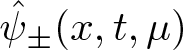 $\hat{\psi}_{\pm}(x,t,\mu)$ have the following symmetry conditions
 \begin{align}
\hat{\psi}_{\pm}(\mu)=\sigma_{1}\hat{\psi}^{*}_{\pm}(\mu^{*})\sigma_{1}=
\sigma_{2}\hat{\psi}_{\pm}(-\mu)\sigma_{2}=\sigma_{1}\hat{\psi}_{\pm}(\frac{1}{\mu})\sigma_{1}.
\end{align}
Proposition 3.3. The Jost eigenfunctions 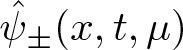 $\hat{\psi}_{\pm}(x,t,\mu)$ possess asymptotic behaviour in the µ-plane
 \begin{align}
\begin{split}
\hat{\psi}_{\pm}(x,t,\mu)&=I+\mathcal {O}(\frac{1}{\mu}),\quad \mu\rightarrow\infty,\\
\hat{\psi}_{\pm}(x,t,\mu)&=I+\mathcal {O}(\mu),\quad \mu\rightarrow0,\\
\hat{\psi}_{\pm}(x,t,\mu)&=
\frac{i}{4(\mu-1)}\alpha_{\pm}(x,t)\Sigma_{1}+\mathcal {O}(1),\quad \mu\rightarrow1,\\
\hat{\psi}_{\pm}(x,t,\mu)&=
-\frac{i}{4(\mu+1)}\alpha_{\pm}(x,t)\Sigma_{2}+\mathcal {O}(1),\quad \mu\rightarrow-1,
\end{split}
\end{align}
there  $\alpha_{\pm}(x,t)\in\mathbb{R}$,
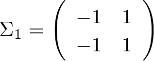 $$\Sigma_{1}=\left(\begin{array}{cc}
-1 & 1 \\
-1 & 1
\end{array}\right)$$ and
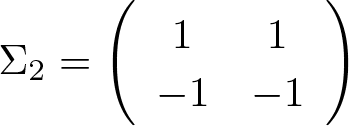 $$\Sigma_{2}=\left(\begin{array}{cc}
1 & 1 \\
-1 & -1
\end{array}\right)$$.
Remark 3.4. It should be noted that the Lax pair (Equation 2.1) for the cCH equation under ZBCs has singularities at points µ = 0, 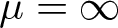 $\mu=\infty$ and branch cut points
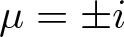 $\mu=\pm i$ in the extended complex µ-plane. Besides, the Lax pair (Equation 3.1) for the cCH equation under NZBCs in addition to possessing the above singularities also has the new singularities at points
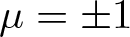 $\mu=\pm1$. Therefore, the asymptotic behaviour of these points should be controlled.
Because 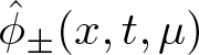 $\hat{\phi}_{\pm}(x,t,\mu)$ are two fundamental matrix solutions of the Lax pair (Equation 3.1), there exists a linear relation between them.
 \begin{align}
\hat{\phi}_{-}(x,t,\mu)=\hat{\phi}_{+}(x,t,\mu)S(\mu),
\end{align}
using the transformation (Equation 3.3), matrix  $S(\mu)$ can be introduced as follows
 \begin{align}
\hat{\psi}_{-}(x,t,\mu)=\hat{\psi}_{+}(x,t,\mu)e^{-p(x,t,\mu)\sigma_{3}}S(\mu)e^{p(x,t,\mu)\sigma_{3}},
\end{align}
there  $\mu\in\mathbb{R},\mu\neq\pm1$. On the basis of symmetry conditions of
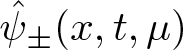 $\hat{\psi}_{\pm}(x,t,\mu)$, the matrix
 $S(\mu)$ can be expressed as
 \begin{align}
S(\mu)=\left(\begin{array}{cc}
a(\mu) & b^{*}(\mu^{*}) \\
b(\mu) & a^{*}(\mu^{*})
\end{array}\right).
\end{align}
Taking into account the properties of the Jost eigenfunctions 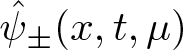 $\hat{\psi}_{\pm}(x,t,\mu)$, we obtain the corresponding properties to the elements
 $a(\mu)$ and
 $b(\mu)$ of the scattering matrix
 $S(\mu)$ as follows.
Proposition 3.5. The scattering data  $a(\mu)$ and
 $b(\mu)$ satisfy the following relations
(i)
$a(\mu)$ is analytic in $\mathbb{C}^{+}$ and continuously extended to $\mathbb{C}^{+}\cup\mathbb{R}$ except the points $\mu=\pm1$, $a(\mu)\rightarrow 1$ as $\mu\rightarrow \infty$,(ii)
$b(\mu)$ is continuous in $\mu\in\mathbb{R}\backslash{\left\{-1,0,1\right\}}$, $b(\mu)\rightarrow 0$ as $\mu\rightarrow \infty$,(iii)
$a(\mu)=\frac{i\beta}{4(\mu-1)}+\mathcal {O}(1)$, $b(\mu)=\frac{i\beta}{4(\mu-1)}+\mathcal {O}(1)$, $\mu\rightarrow1$, $\beta\in\mathbb{R}$,(iv)
$a(\mu)=\frac{i\beta}{4(\mu+1)}+\mathcal {O}(1)$, $b(\mu)=-\frac{i\beta}{4(\mu+1)}+\mathcal {O}(1)$, $\mu\rightarrow-1$, $\beta\in\mathbb{R}$,(v)
$a^{*}(\mu^{*})=a(-\mu)=a(\frac{1}{\mu})$, $b^{*}(\mu^{*})=-b(-\mu)=b(\frac{1}{\mu})$,(vi)
$|a(\mu)|^{2}-|b(\mu)|^{2}=1$, $\mu\in\mathbb{R}$, $\mu\neq\pm1$.



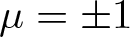
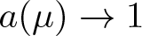
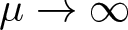


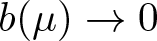
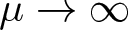


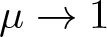



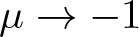




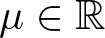
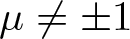
Remark 3.6. It should be noted that β ≠ 0 of proposition 3.5 is generic and when β = 0, we have 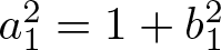 $a_{1}^{2}=1+b_{1}^{2}$ with
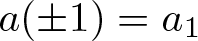 $a(\pm1)=a_{1}$,
 $b(\pm1)=\pm b_{1}$,
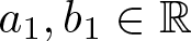 $a_{1}, b_{1}\in\mathbb{R}$. According to (Equation 3.12),
 $\alpha_{+}(x,t)=(a_{1}-b_{1})\alpha_{-}(x,t)$.
The analytic properties of 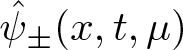 $\hat{\psi}_{\pm}(x,t,\mu)$ stated above allow rewriting the relation (Equation 3.12) as a sectionally meromorphic matrix.
3.2. RH problem
A piecewise meromorphic  $2\times2$-matrix valued function
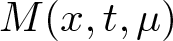 $M(x,t,\mu)$ is introduced as follows
 \begin{align}
M(x,t;\mu)=\left\{\begin{array}{ll}
\left( \frac{\hat{\psi}_{-,1}(x,t;\mu)}{a(\mu)}, \hat{\psi}_{+,2}(x,t;\mu)\right), &\text{as } Im\mu \gt 0,\\[12pt]
\left( \hat{\psi}_{+,1}(x,t;\mu),\frac{\hat{\psi}_{-,2}(x,t;\mu)}{a^{*}(\mu^{*})}\right) , &\text{as } Im\mu \lt 0.\\
\end{array}\right.
\end{align}
At the same time, we define the reflection coefficient
 \begin{align}
r(\mu)=\frac{b(\mu)}{a(\mu)},\quad \mu\in\mathbb{R}.
\end{align}
RHP 3.7.
Find a matrix  $M(\mu)=M(x,t,\mu)$ satisfies the following conditions
(i) Analyticity: the matrix
$M(\mu)$ is a meromorphic function in $\mathbb{C}\backslash\mathbb{R}$.(ii) Jump condition:
(3.16)\begin{align}
M_{+}(x,t,\mu)=M_{-}(x,t,\mu)G(x,t,\mu),\quad \mu\in\mathbb{R}, \mu\neq\pm1,
\end{align}where
(3.17)\begin{align}
G(x,t,\mu)=e^{-p(x,t,\mu)\sigma_{3}}G_{0}(\mu)e^{p(x,t,\mu)\sigma_{3}},
\end{align}and
(3.18)\begin{align}
G_{0}(\mu)=\left(\begin{array}{cc}
1-r(\mu)r^{*}(\mu^{*}) & -r^{*}(\mu^{*}) \\
r(\mu) & 1
\end{array}\right),
\end{align}$p(x,t,\mu)$ is shown in (Equation 3.7).(iii) Normalization condition:
(3.19)\begin{align}
M(x,t,\mu)\rightarrow I,\quad \mu\rightarrow \infty.
\end{align}(iv) Singularity condition:
(3.20)\begin{align}
M(x,t,\mu)=\begin{cases}
\frac{i\alpha_{+}(x,t)}{4(\mu-1)}\left(\begin{array}{cc}
-D & 1 \\
-D & 1
\end{array}\right)+\mathcal {O}(1),\quad \mu\rightarrow1,\\[12pt]
-\frac{i\alpha_{+}(x,t)}{4(\mu+1)}\left(\begin{array}{cc}
D & 1 \\
-D & -1
\end{array}\right)+\mathcal {O}(1),\quad \mu\rightarrow-1,\\
\end{cases}
\end{align}where
$\alpha_{+}(x,t)\in\mathbb{R}$ and $Im\mu \gt 0$,
(3.21)\begin{align}
D:=\left\{
\begin{array}{ll}
0,\quad \beta\neq0,\\[12pt]
\frac{a_{1}+b_{1}}{a_{1}},\quad \beta=0,\\
\end{array}
\right.
\end{align}$a_{1}=a(1)$, $b_{1}=b(1)$ and $\beta:=-2i\lim\limits_{\mu \to 1}(\mu-1)a(\mu)$.(v) Symmetry conditions:
(3.22)\begin{align}
M(\mu)=\sigma_{1}M^{*}(\mu^{*})\sigma_{1}=\sigma_{2}M(-\mu)\sigma_{2}=\sigma_{1}M(\frac{1}{\mu})\sigma_{1}.
\end{align}(vi)
$\det M(x,t,\mu)\equiv1$.


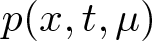



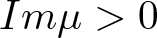

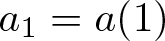
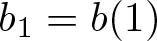



We substitute Eqs. (Equation 3.6) into Lax pair (Equation 3.5a) and take the new transformation
 \begin{align}
\hat{\psi}_{0}=\hat{\varphi}e^{\hat{J}_{0}},
\end{align}
with
 \begin{align}
p_{0}=\frac{i(\mu^{2}-1)}{4\mu}x-\frac{4i(\mu^{2}-1)\mu}{(\mu^{2}+1)^{2}}t,
\end{align}
there 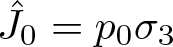 $\hat{J}_{0}=p_{0}\sigma_{3}$, the Lax pair can be converted to
 \begin{align}
&\hat{\psi}_{0x}+[\hat{J}_{0x},\hat{\psi}_{0}]=\hat{X}_{0}\hat{\psi}_{0},
\end{align}
 \begin{align}
&\hat{\psi}_{0t}+[\hat{J}_{0t},\hat{\psi}_{0}]=\hat{T}_{0}\hat{\psi}_{0},
\end{align}
with
 \begin{align*}
\hat{X_{0}}(x,t,\mu)&=-\frac{(\mu^{2}+1)\sqrt{8\mu^{2}-(\mu^{2}+1)^{2}}(\hat{m}-1)}{8|\mu|(\mu^{2}-1)}\sigma_{2}\\
&+\left(\frac{i((\mu^{2}+1)^{2}-8\mu^{2})(\hat{m}-1)}{8\mu(\mu^{2}-1)}-\frac{i(\hat{m}-1)(\mu^{2}-1)}{4\mu}
\right)\sigma_{3},
\end{align*}
 \begin{align*}
\hat{T_{0}}(x,t,\mu)=\frac{i(\mu^{2}-1)}{4\mu}\hat{R}\hat{m}\sigma_{3}
+\frac{i(\mu^{2}-1)}{2\mu}\hat{u}\sigma_{3}+\hat{T}(x,t,\mu).
\end{align*}
Then the Jost solutions of Equation 3.25a are expressed as
 \begin{align}
\hat{\psi}_{0\pm}(x,t,\mu)=I+\int_{\pm\infty}^{x}e^{-\frac{i(\mu^{2}-1)}{4\mu}(x-\xi)\hat{\sigma}_{3}}
\left[\hat{X}_{0}(\xi,t,\mu)\hat{\psi}_{0\pm}(\xi,t,\mu)\right]d\xi.
\end{align}
Utilizing the transformation (Equation 3.23), there exist matrices  $r_{\pm}(\mu)$ satisfying
 \begin{align}
\hat{\psi}_{\pm}(x,t,\mu)=\hat{\psi}_{0\pm}(x,t,\mu)e^{-\hat{J}_{0}}r_{\pm}(\mu)e^{\hat{J}}.
\end{align}
Thus  $r_{\pm}(\mu)=e^{\hat{J}_{0}(\pm\infty,t,\mu)-\hat{J}(\pm\infty,t,\mu)}$. On the basis of (Equation 3.7) and (Equation 3.24),
 \begin{align}
r_{+}(\mu)=I, \quad
r_{-}(\mu)=e^{\frac{i(\mu^{2}-1)}{4\mu}\int_{-\infty}^{+\infty}(\hat{m}(\xi,t)-1)d\xi\sigma_{3}}.
\end{align}
Because  $\hat{X}_{0}(x,t,\pm i)\equiv0$, making use of (Equation 3.26) and
 $a(\mu)=\det(\hat{\psi}_{-,1},\hat{\psi}_{+,2})$, we have
 \begin{align}
M(x,t,i)=\left(\begin{array}{cc}
e^{\frac{1}{2}\int_{x}^{+\infty}(\hat{m}(\xi,t)-1)d\xi} & 0 \\
0 & e^{-\frac{1}{2}\int_{x}^{+\infty}(\hat{m}(\xi,t)-1)d\xi}
\end{array}\right),
\end{align}
with symmetry of 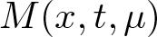 $M(x,t,\mu)$, we can obtain
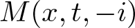 $M(x,t,-i)$. Besides, the symmetry conditions (Equation 3.22) indicate M(i) is a diagonal matrix with real entries, taking into account
 $\det M\equiv1$, there exists
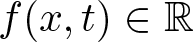 $f(x,t)\in\mathbb{R}$ such that
 $M_{11}(x,t,i)=f(x,t)$ and
 $M_{22}(x,t,i)=\frac{1}{f(x,t)}$.
Based on the new space variable  $y(x,t)=x-\int_{x}^{+\infty}(\hat{m}(\xi,t)-1)d\xi$ and
 $\tilde{M}(y,t,\mu)=M(x,t,\mu)$, we have a new RH problem.
RHP 3.8.
Find a matrix  $\tilde{M}(\mu)=\tilde{M}(y,t,\mu)$ satisfies the following conditions
(i) Analyticity: the matrix
$\tilde{M}(\mu)$ is a meromorphic function in $\mathbb{C}\backslash\mathbb{R}$.(ii) Jump condition:
(3.30)\begin{align}
\tilde{M}_{+}(y,t,\mu)=\tilde{M}_{-}(y,t,\mu)\tilde{G}(y,t,\mu),\quad \mu\in\mathbb{R}, \mu\neq\pm1,
\end{align}where
(3.31)\begin{align}
\tilde{G}(y,t,\mu)=e^{-\tilde{p}(y,t,\mu)\sigma_{3}}G_{0}(\mu)e^{\tilde{p}(y,t,\mu)\sigma_{3}},
\end{align}(3.32)\begin{align}
\tilde{p}(y,t,\mu)=\frac{i(\mu^{2}-1)}{4\mu}y-\frac{4i(\mu^{2}-1)\mu}{(\mu^{2}+1)^{2}}t,
\end{align}$G_{0}(\mu)$ defined by (Equation 3.18).(iii) Normalization condition:
(3.33)\begin{align}
\tilde{M}(y,t,\mu)\rightarrow I,\quad \mu\rightarrow \infty.
\end{align}(iv) Singularity condition:
(3.34)\begin{align}
\tilde{M}(y,t,\mu)=\begin{cases}
\frac{i\tilde{\alpha}_{+}(y,t)}{4(\mu-1)}\left(\begin{array}{cc}
-D & 1 \\
-D & 1
\end{array}\right)+\mathcal {O}(1),\quad \mu\rightarrow1,\\[12pt]
-\frac{i\tilde{\alpha}_{+}(y,t)}{4(\mu+1)}\left(\begin{array}{cc}
D & 1 \\
-D & -1
\end{array}\right)+\mathcal {O}(1),\quad \mu\rightarrow-1,\\
\end{cases}
\end{align}with some
$\tilde{\alpha}_{+}(y,t)\in\mathbb{R}$ and $Im\mu \gt 0$.(v) Symmetry conditions:
(3.35)\begin{align}
\tilde{M}(\mu)=\sigma_{1}\tilde{M}^{*}(\mu^{*})\sigma_{1}=\sigma_{2}\tilde{M}(-\mu)\sigma_{2}=\sigma_{1}\tilde{M}(\frac{1}{\mu})\sigma_{1}.
\end{align}(vi)
$\det\tilde{M}(y,t,\mu)\equiv1$.


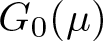



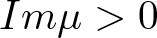


The implicit expression of the potential function u under NZBCs is constructed by using the solution of RH problem.
Theorem 3.9
Consider that 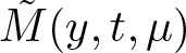 $\tilde{M}(y,t,\mu)$ is a solution of RH problem 3.8, according to the definition of
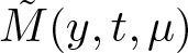 $\tilde{M}(y,t,\mu)$ at
 $\mu=i$, we make
 $\hat{\Phi}_{1}(x(y,t),t)=\tilde{\Phi}_{1}(y,t)=\tilde{M}_{11}(y,t,i)+\tilde{M}_{21}(y,t,i)$ and
 $\hat{\Phi}_{2}(x(y,t),t)=\tilde{\Phi}_{2}(y,t)=\tilde{M}_{12}(y,t,i)+\tilde{M}_{22}(y,t,i)$, then the solution
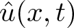 $\hat{u}(x,t)$ of Cauchy problem (Equation 1.3) has the following representation
 \begin{align}
\left(\hat{R}+\frac{2\hat{u}}{\hat{m}}\right)(\hat{m}+1)=\partial_{t}\ln\frac{\tilde{\Phi}_{1}(y,t)}{\tilde{\Phi}_{2}(y,t)},
\end{align}
with
 \begin{align*}
\hat{R}=\hat{u}^{2}-\hat{u}^{2}_{x}+2\hat{u},\quad
\hat{m}=\hat{u}-\hat{u}_{xx}+1.
\end{align*}
Proof. Considering the new notations  $\tilde{R}(y,t)=\hat{R}(x(y,t),t)$,
 $\tilde{m}(y,t)=\hat{m}(x(y,t),t)$,
 $\tilde{u}(y,t)=\hat{u}(x(y,t),t)$ and
 $\tilde{u}_{x}(y,t)=\hat{u}_{x}(x(y,t),t)$, with regard to
 $x(y(x,t),t)=x$, we have
 \begin{align}
\partial_{t}(x(y(x,t),t))=x_{y}(y,t)y_{t}(x,t)+x_{t}(y,t)=0.
\end{align}
Since  $y(x,t)=x-\int_{x}^{+\infty}(\hat{m}(\xi,t)-1)d\xi$, then
 \begin{align}
x_{y}(y,t)=\frac{1}{\tilde{m}(y,t)}.
\end{align}
Based on  $\hat{m}_{t}=-(\hat{m} \hat{R})_{x}-2\hat{u}_{x}$ and unite (Equation 3.37)–(Equation 3.38), we have
 \begin{align}
x_{t}(y,t)=\tilde{R}(y,t)+\frac{2\tilde{u}(y,t)}{\tilde{m}(y,t)}.
\end{align}
By (Equation 3.29), we have
 \begin{align}
\hat{\Phi}_{1}(x,t)=e^{\frac{1}{2}\int_{x}^{+\infty}(\tilde{m}(\xi,t)-1)d\xi},\quad
\hat{\Phi}_{2}(x,t)=e^{-\frac{1}{2}\int_{x}^{+\infty}(\tilde{m}(\xi,t)-1)d\xi},
\end{align}
then
 \begin{align}
x=y(x,t)+\ln\frac{\tilde{\Phi}_{1}(y,t)}{\tilde{\Phi}_{2}(y,t)}.
\end{align}
Differential equation (Equation 3.41) with respect to t,
 \begin{align}
x_{t}=-(\tilde{R}(y,t)\tilde{m}(y,t)+2\tilde{u}(y,t))+\partial_{t}\ln\frac{\tilde{\Phi}_{1}(y,t)}{\tilde{\Phi}_{2}(y,t)},
\end{align}
making further calculation, we can get (Equation 3.36), then the theorem 3.9 can be proved.
Next, in order to obtain the solution of Lax pair (Equation 3.1) represented by the new variable 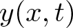 $y(x,t)$, using the gauge transformation
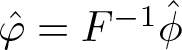 $\hat{\varphi}=F^{-1}\hat{\phi}$, there we have
 $\tilde{\varphi}(y,t,\lambda)=\hat{\varphi}(x,t,\lambda)$. Taking (Equation 3.38) and (Equation 3.39) into consideration, the Lax pair (Equation 3.1) turns into
 \begin{align}
\tilde{\varphi}_{y}=\tilde{U}\tilde{\varphi},\quad \tilde{\varphi}_{t}=\tilde{V}\tilde{\varphi},
\end{align}
there  $\tilde{U}=\tilde{X}-ik\sigma_{3}$ and
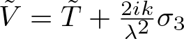 $\tilde{V}=\tilde{T}+\frac{2ik}{\lambda^{2}}\sigma_{3}$. Then we change the parameters to µ and expanding
 $\tilde{X}$ and
 $\tilde{T}$ at the singularities
 $\mu=\pm1, \pm i$
 \begin{align}
&\tilde{\varphi}_{y}+\frac{i(\mu^{2}-1)}{4\mu}\sigma_{3}\tilde{\varphi}=\tilde{X}_{1}\tilde{\varphi},
\end{align}
 \begin{align}
&\tilde{\varphi}_{t}-\frac{4i(\mu^{2}-1)\mu}{(\mu^{2}+1)^{2}}\sigma_{3}\tilde{\varphi}=\tilde{T}_{1}\tilde{\varphi},
\end{align}
with
 \begin{align*}
\tilde{X}_{1}=-\frac{iv_{1}}{\mu-1}\Sigma_{1}+\frac{iv_{1}}{\mu+1}\Sigma_{2}+v_{1}\sigma_{2},
\end{align*}
 \begin{align*}
\tilde{T}_{1}=-\frac{iv_{2}}{\mu-1}\Sigma_{1}+\frac{iv_{2}}{\mu+1}\Sigma_{2}
+\frac{v_{3}\Delta_{1}+v_{4}\Delta_{2}}{\mu-i}+
\frac{v_{3}\Delta_{2}+v_{4}\Delta_{1}}{\mu+i},
\end{align*}
where 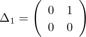 $$\Delta_{1}=\left(\begin{array}{cc}
0 & 1 \\
0 & 0
\end{array}\right)$$,
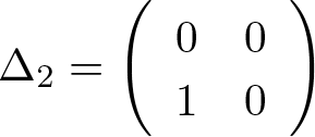 $$\Delta_{2}=\left(\begin{array}{cc}
0 & 0 \\
1 & 0
\end{array}\right)$$, Σ1 and Σ2 are shown in proposition 3.3. Besides, we also have
 $v_{1}(y,t)=-\frac{\tilde{m}-1}{2\tilde{m}}$,
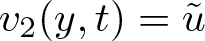 $v_{2}(y,t)=\tilde{u}$,
 $v_{3}(y,t)=-\tilde{u}-\tilde{u}_{x}$, and
 $v_{4}(y,t)=\tilde{u}-\tilde{u}_{x}$.
Proposition 3.10. Assume 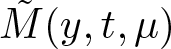 $\tilde{M}(y,t,\mu)$ is a solution of RH problem 3.8, then
 \begin{align}
\tilde{\varphi}(y,t,\mu)=\tilde{M}(y,t,\mu)e^{-\tilde{p}(y,t,\mu)\sigma_{3}}
\end{align}
satisfies the Lax pair (Equation 3.44a), there 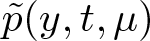 $\tilde{p}(y,t,\mu)$ is shown in (Equation 3.32).
(i) First of all, we think about the y differential part of the Lax pair (Equation 3.44a). From (Equation 3.30) and (Equation 3.45), we can obtain
(3.46)\begin{align}
\tilde{\varphi}_{y}\tilde{\varphi}^{-1}=\tilde{M}_{y}\tilde{M}^{-1}-
\tilde{p}_{y}\tilde{M}\sigma_{3}\tilde{M}^{-1},
\end{align}then the possible subsistent singularities are
$\mu=0,1,-1,\infty$. Now we estimate $\tilde{\varphi}_{y}\tilde{\varphi}^{-1}$ at these points. On the basis of the symmetry conditions (Equation 3.35), expanding $\tilde{M}(y,t,\mu)$ with µ at $\mu\rightarrow\infty$
(3.47)\begin{align}
\tilde{M}=I+\frac{1}{\mu}[w\sigma_{3}+\tilde{w}(\Delta_{1}+\Delta_{2})]+\mathcal {O}(\mu^{-2}),\quad \mu\rightarrow\infty,
\end{align}where
$w=w(y,t)\in i\mathbb{R}$, $\tilde{w}=\tilde{w}(y,t)\in \mathbb{R}$. Considering the expansion of $\tilde{p}_{y}$ at $\mu\rightarrow\infty$, $\mu\rightarrow0$, and $\mu\rightarrow\pm1$, we have
(3.48)\begin{align}
\begin{split}
\tilde{\varphi}_{y}\tilde{\varphi}^{-1}&=-\frac{i\mu}{4}\sigma_{3}-
\frac{\tilde{w}}{2}\sigma_{2}+\mathcal {O}(\mu^{-1}),\quad \mu\rightarrow\infty.\\
\tilde{\varphi}_{y}\tilde{\varphi}^{-1}&=\frac{i}{4\mu}\sigma_{3}+
\frac{\tilde{w}}{2}\sigma_{2}+\mathcal {O}(\mu),\quad \mu\rightarrow 0.\\
\tilde{\varphi}_{y}\tilde{\varphi}^{-1}&=-\frac{i\alpha_{1}}{\mu-1}\Sigma_{1}+\mathcal {O}(1),\quad \mu\rightarrow 1,\\
\tilde{\varphi}_{y}\tilde{\varphi}^{-1}&=\frac{i\alpha_{1}}{\mu+1}\Sigma_{2}+\mathcal {O}(1),\quad \mu\rightarrow -1.
\end{split}
\end{align}Uniting (Equation 3.48), since
$\tilde{M}(y,t,i)$ is a diagonal matrix,
\begin{align*}
-\frac{i\alpha_{1}}{i-1}\Sigma_{1}+
\frac{i\alpha_{1}}{i+1}\Sigma_{2}-\frac{\tilde{w}}{2}\sigma_{2}
\end{align*}is also diagonal, then
$\frac{\tilde{w}(y,t)}{2}=-\alpha_{1}(y,t)$, and the y differential part of the Lax pair (Equation 3.44a) can be attained, where $v_{1}(y,t)=\alpha_{1}(y,t)$.(ii) Secondly, using the similar method, we think over the t differential part of the Lax pair (Equation 3.44a). Due to
(3.49a)\begin{align}
&\tilde{p}_{t}(\mu)=\frac{2}{(\mu-i)^{2}}-\frac{2i}{\mu-i}+\mathcal {O}(1),\quad \mu\rightarrow i,
\end{align}(3.49b)\begin{align}
&\tilde{p}_{t}(\mu)=-\frac{2}{(\mu+i)^{2}}-\frac{2i}{\mu+i}+\mathcal {O}(1),\quad \mu\rightarrow -i,
\end{align}then the possible subsistent singularities are
$\mu=0,1,-1,i,-i,\infty$. Now estimating $\tilde{\varphi}_{t}\tilde{\varphi}^{-1}=
\tilde{M}_{t}\tilde{M}^{-1}-\tilde{p}_{t}\tilde{M}\sigma_{3}\tilde{M}^{-1}$ at these points at $\mu\rightarrow \infty$, $\mu\rightarrow0$ and $\mu\rightarrow\pm1$ we have $\tilde{p}_{t}(\mu)=\mathcal {O}(\mu^{-1})$, such that,
(3.50)\begin{align}
\begin{split}
\tilde{\varphi}_{t}\tilde{\varphi}^{-1}&=\mathcal {O}(\mu^{-1}),\quad\mu\rightarrow\infty.\\
\tilde{\varphi}_{t}\tilde{\varphi}^{-1}&=\mathcal {O}(\mu),\quad \mu\rightarrow 0.\\
\tilde{\varphi}_{t}\tilde{\varphi}^{-1}&=-\frac{i\alpha_{2}}{\mu-1}\Sigma_{1}+\mathcal {O}(1),\quad \mu\rightarrow 1,\\
\tilde{\varphi}_{t}\tilde{\varphi}^{-1}&=\frac{i\alpha_{2}}{\mu+1}\Sigma_{2}+\mathcal {O}(1),\quad \mu\rightarrow -1.
\end{split}
\end{align}Subsequently, on the basis of symmetries (Equation 3.35), estimating
$\tilde{M}(\mu)$ at $\mu\rightarrow i$,
(3.51)\begin{align}
\tilde{M}=\left(\begin{array}{cc}
f_{1} & 0 \\
0 & f_{1}^{-1}
\end{array}\right)+\left(\begin{array}{cc}
0 & f_{2} \\
f_{3} & 0
\end{array}\right)(\mu-i)+\mathcal {O}((\mu-i)^{2}).
\end{align}We have
(3.52)\begin{align}
\tilde{\varphi}_{t}\tilde{\varphi}^{-1}=
-\frac{2}{(\mu-i)^{2}}\sigma_{3}+\frac{2}{\mu-i}\left(\begin{array}{cc}
i & 2f_{2}f_{1} \\
-2f_{3}f_{1}^{-1} & -i
\end{array}\right)+\mathcal {O}(1).
\end{align}By symmetry, at
$\mu\rightarrow -i$,
(3.53)\begin{align}
\tilde{\varphi}_{t}\tilde{\varphi}^{-1}=
\frac{2}{(\mu+i)^{2}}\sigma_{3}+\frac{2}{\mu+i}\left(\begin{array}{cc}
i & -2f_{3}f_{1}^{-1} \\
2f_{2}f_{1} & -i
\end{array}\right)+\mathcal {O}(1).
\end{align}There
$f_{j}=f_{j}(y,t)$ $(j=1,2,3)$. Uniting (Equation 3.50)–(Equation 3.53), we have $g_{1}(y,t)=2f_{2}(y,t)f_{1}(y,t)$ and $g_{2}(y,t)=-2f_{3}(y,t)f_{1}^{-1}(y,t)$ are holomorphic functions in the whole complex µ-plane and vanished as $\mu\rightarrow \infty$. After that, the t differential part of the Lax pair (Equation 3.44a) can be attained, there $v_{2}(y,t)=\alpha_{2}(y,t)$.


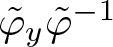
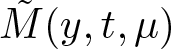
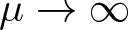




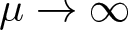
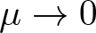
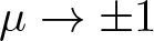

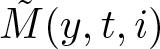







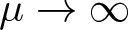
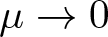
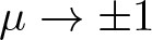



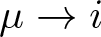


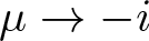

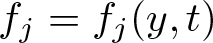
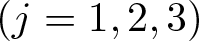


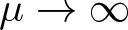

For the sake of testifying the compatibility conditions  $\tilde{U}_{t}-\tilde{V}_{y}+[\tilde{U},\tilde{V}]=0$ of Lax pair (Equation 3.43) can be deduced Eq. (Equation 1.3) with variables (y, t), we have the theorem 3.11 and theorem 3.12.
Theorem 3.11
Equation (Equation 1.3) with variables (y, t) can be shown as follows
 \begin{align}
\tilde{m}^{-1}_{t}(y,t)=2\tilde{u}_{x}(y,t)-\frac{2\tilde{u}\tilde{m}_{x}}{\tilde{m}^{3}}(y,t)
+\frac{2\tilde{u}_{x}}{\tilde{m}^{2}}(y,t),
\end{align}
with
 \begin{align*}
\tilde{m}(y,t)=\tilde{u}(y,t)-\tilde{u}_{xx}(y,t)+1,\quad
x_{y}(y,t)=\tilde{m}^{-1}(y,t).
\end{align*}
Proof. According to equations  $\hat{m}_{t}=-(\hat{m} \hat{R})_{x}-2\hat{u}_{x}$,
 $x_{t}(y,t)=\tilde{R}(y,t)+\frac{2\tilde{u}(y,t)}{\tilde{m}(y,t)}$ and
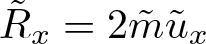 $\tilde{R}_{x}=2\tilde{m}\tilde{u}_{x}$,
 \begin{align*}
\tilde{m}_{t}(y,t)&=\tilde{m}_{x}(x(y,t),t)x_{t}(y,t)+\tilde{m}_{t}(x(y,t),t)\\
&=\left(-\frac{2\tilde{u}\tilde{m}_{x}}{\tilde{m}^{3}}+\frac{2\tilde{u}_{x}}{\tilde{m}^{2}}\right)
(-\tilde{m}^{2})+2\tilde{u}_{x}(-\tilde{m}^{2}),
\end{align*}
then we have Eq. (Equation 3.54), and the theorem 3.11 can be proved.
Theorem 3.12
It can be demonstrable that the functions 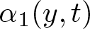 $\alpha_{1}(y,t)$,
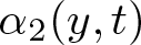 $\alpha_{2}(y,t)$,
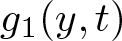 $g_{1}(y,t)$, and
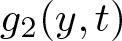 $g_{2}(y,t)$ of proposition 3.10 content the following algebraic system
 \begin{align}
&\alpha_{1t}+(g_{1}+g_{2})=0,
\end{align}
 \begin{align}
&\alpha_{2}+(g_{1}-g_{2})=0,
\end{align}
 \begin{align}
&(g_{1}-g_{2})_{y}-(1+2\alpha_{1})(g_{1}+g_{2})=0,
\end{align}
 \begin{align}
&(g_{1}+g_{2})_{y}+2\alpha_{1}-(1+2\alpha_{1})(g_{1}-g_{2})=0,
\end{align}
then the compatibility conditions of Lax pair (Equation 3.43) can be satisfied.
Proof. By the definitions about 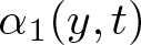 $\alpha_{1}(y,t)$,
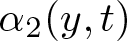 $\alpha_{2}(y,t)$,
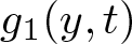 $g_{1}(y,t)$, and
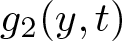 $g_{2}(y,t)$ which are shown in proposition 3.10, there
 $g_{1}(y,t)=2f_{2}(y,t)f_{1}(y,t)$,
 $g_{2}(y,t)=-2f_{3}(y,t)f_{1}^{-1}(y,t)$. Subsequently, estimating the compatibility conditions
 $\tilde{U}_{t}-\tilde{V}_{y}+[\tilde{U},\tilde{V}]=0$ at these points
 $\mu=0,1,-1,i,-i,\infty$, the theorem 3.12 can be proved.
Proposition 3.13. In compliance with proposition 3.10 and theorem 3.11, the relations of  $\tilde{m}$ and
 $\tilde{\mu}$ with notations
 $\left\{\alpha_{1}, \alpha_{2}, g_{1}, g_{2}\right\}$ can be available as follows
 \begin{align}
\tilde{m}=\frac{1}{1+2\alpha_{1}},\quad
\tilde{u}=\alpha_{2},
\end{align}
with the conditions  $x_{y}=1+2\alpha_{1}$ and
 $(\alpha_{1}\alpha_{2})_{x}=-\frac{\alpha_{2x}}{2}$, we can derive Eq. (Equation 3.54) from (Equation 3.55a)–(Equation 3.55d).
Proof. Actually, (Equation 3.55a) can be obtained by (Equation 3.54), and from (Equation 3.55c) we have
 \begin{align*}
\tilde{u}_{x}=\tilde{u}_{y}x^{-1}_{y}=-(g_{1}+g_{2}).
\end{align*}
According to
 \begin{align*}
\tilde{m}=\tilde{u}-(\tilde{u}_{x})_{y}\tilde{m}+1,
\end{align*}
we have
 \begin{align*}
\frac{1}{1+2\alpha_{1}}=-(g_{1}-g_{2})+(g_{1}+g_{2})_{y}\frac{1}{1+2\alpha_{1}}+1,
\end{align*}
which is Eq. (Equation 3.55d).
Combining Eqs. (Equation 3.56) and (Equation 3.55b), we can further obtain the relationship between the solution of cCH equation and the RH problem as shown in (Equation 3.82).
3.3. Single high-order pole solutions
In order to obtain a pure soliton solution, this section we will consider the reflectionless situation, i.e., 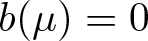 $b(\mu)=0$
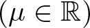 $(\mu\in\mathbb{R})$. Then
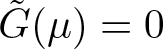 $\tilde{G}(\mu)=0$ for
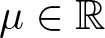 $\mu\in\mathbb{R}$. Let
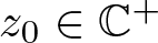 $z_{0}\in\mathbb{C}^{+}$ be the N-order zero point of the scattering data
 $a(\mu)$, then
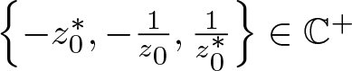 $\left\{-z_{0}^{*}, -\frac{1}{z_{0}}, \frac{1}{z_{0}^{*}}\right\}\in\mathbb{C}^{+}$ are also the N-order zero points of the scattering data
 $a(\mu)$. Furthermore,
 $\left\{z_{0}^{*}, -z_{0}, -\frac{1}{z_{0}^{*}}, \frac{1}{z_{0}}\right\}\in\mathbb{C}^{-}$ are the N-order zero points of the scattering data
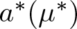 $a^{*}(\mu^{*})$. The discrete spectrum is the set
 $\mathcal{X}=\left\{\pm z_{0}, \pm z^{*}_{0}, \pm\frac{1}{z_{0}}, \pm\frac{1}{z^{*}_{0}}\right\}$, which is same as the case in figure 1. Taking
 $w_{1}=z_{0}$,
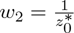 $w_{2}=\frac{1}{z^{*}_{0}}$, the scattering data
 $a(\mu)$ has the following form
 \begin{align}
a(\mu)=\prod_{j=1}^{2}(\mu-w_{j})^{N}(\mu+w^{*}_{j})^{N}a_{0}(\mu),
\end{align}
where 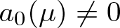 $a_{0}(\mu)\neq0$ for all
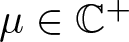 $\mu\in\mathbb{C}^{+}$. Therefore, from the definition of
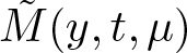 $\tilde{M}(y,t,\mu)$, it can be seen that
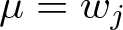 $\mu=w_{j}$ and
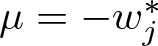 $\mu=-w^{*}_{j}$
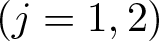 $(j=1,2)$ are N-order pole points of
 $\tilde{M}_{11}$. Simultaneously,
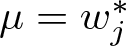 $\mu=w^{*}_{j}$ and
 $\mu=-w_{j}$
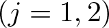 $(j=1,2)$ are N-order pole points of
 $\tilde{M}_{12}$. According to the definitions of (Equation 3.11) and (Equation 3.12), under the new scale
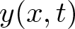 $y(x,t)$, we define
 $\check{\phi}_{\pm}(y,t,\mu)=\hat{\phi}_{\pm}(x,t,\mu)$ and
 $\check{\psi}_{\pm}(y,t,\mu)=\hat{\psi}_{\pm}(x,t,\mu)$ and obtain the following relationships
 \begin{equation}
\check{\phi}_-(y,t,\mu)=\check{\phi}_+(y,t,\mu)S(\mu),
\end{equation}
and
 \begin{equation}
\check{\psi}_-(y,t,\mu)e^{-it\theta(\mu)\sigma_{3}}=\check{\psi}_+(y,t,\mu)e^{-it\theta(\mu)\sigma_{3}}S(\mu),
\end{equation}
there we redefine relation  $\tilde{p}(\mu)=it\theta(\mu)$,
 $\tilde{p}(\mu)$ is shown in (Equation 3.32). Under the assumption that
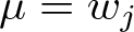 $\mu=w_{j}$
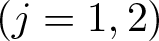 $(j=1,2)$ are N-order zero points of
 $a(\mu)$, from the following two relations, we have a Wronskian form
 \begin{equation}
a(\mu)=Wr(\check{\phi}_{-1},\check{\phi}_{+2}),
\end{equation}
then  $a(\mu)$ vanishes to N-order at zero points wj
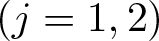 $(j=1,2)$, there exist complex constants
 $b_{j,s}$
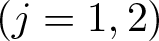 $(j=1,2)$
 $(s=1,2,\cdots,N)$ satisfy the follows
 \begin{equation}
\frac{\partial^{m}[\check{\phi}_+(y,t,w_{j})]_{2}}{\partial\mu^{m}}=\sum^{m}_{l=0}\left(\begin{array}{c}
m \\
l
\end{array}\right)
b_{j,m-l+1}\frac{\partial^{l}[\check{\phi}_-(y,t,w_{j})]_{1}}{\partial\mu^{l}},
\end{equation}
and
 \begin{equation}
\frac{\partial^{m}[\check{\psi}_+(y,t,w_{j})]_{2}}{\partial\mu^{m}}=\sum^{m}_{l=0}\left(\begin{array}{c}
m \\
l
\end{array}\right)
b_{j,m-l+1}\frac{\partial^{l}[\check{\psi}_-(y,t,w_{j})]_{1}e^{2it\theta(w_{j})}}{\partial\mu^{l}},
\end{equation}
with  $m=0,1,\ldots,N-1$. From the normalization condition of RH problem 3.8, one can set
 \begin{align}
&\tilde{M}_{11}=1+\sum_{j=1}^{2}\sum_{s=1}^{N}
\left(\frac{1}{(\mu-w_{j})^{s}}+\frac{(-1)^{s}}{(\mu+w^{*}_{j})^{s}}\right)F_{j,s}
-\frac{i\tilde{\alpha}_{+}(y,t)}{4(\mu-1)}D-\frac{i\tilde{\alpha}_{+}(y,t)}{4(\mu+1)}D,
\end{align}
 \begin{align}
&\tilde{M}_{12}=\sum_{j=1}^{2}\sum_{s=1}^{N}
\left(\frac{1}{(\mu-w^{*}_{j})^{s}}+\frac{(-1)^{s+1}}{(\mu+w_{j})^{s}}\right)G_{j,s}
+\frac{i\tilde{\alpha}_{+}(y,t)}{4(\mu-1)}-\frac{i\tilde{\alpha}_{+}(y,t)}{4(\mu+1)},
\end{align}
where D is shown in (Equation 3.21) and  $\tilde{\alpha}_{+}(y,t)\in\mathbb{R}$. Besides,
 $F_{j,s}=F_{j,s}(y,t)$ and
 $G_{j,s}=G_{j,s}(y,t)$ are undetermined functions. Once these functions are solved, the solution of cCH equation will be acquired. To address this problem, making use of Taylor series expansion, one has
 \begin{align}
&e^{2it\theta(\mu)}=\sum_{l=0}^{+\infty}\zeta_{j,l}(y,t)(\mu-w_{j})^{l},
\end{align}
 \begin{align}
\zeta_{j,l}(y,t)=\lim_{\mu\rightarrow w_{j}}\frac{1}{l!}\frac{\partial^{l}}{\partial \mu^{l}}e^{2it\theta(\mu)}.
\end{align}
It can be obtained that the coefficient of item 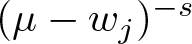 $(\mu-w_{j})^{-s}$ of function
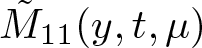 $\tilde{M}_{11}(y,t,\mu)$ is
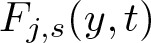 $F_{j,s}(y,t)$. Now we extend the residue theorem by combining (Equation 3.59) and (Equation 3.62) and obtain the following relations
 \begin{align}
\begin{split}
F_{j,s}&=(-1)^{m}\frac{i\tilde{\alpha}_{+}(y,t)}{4}\sum_{l=s}^{N}\sum_{m=0}^{l-s}
\left(\frac{r_{j,l}\zeta_{j,l-s-m}}{(w_{j}-1)^{m+1}}-\frac{r_{j,l}\zeta_{j,l-s-m}}{(w_{j}+1)^{m+1}}\right)\\
&+\sum_{l=s}^{N}\sum_{m=0}^{l-s}\sum_{p=1}^{2}\sum_{q=1}^{N}
\left(
\begin{array}{c}
q+m-1\\
m \\
\end{array}
\right)
r_{j,l}\zeta_{j,l-s-m}\times\\
&\left\{\frac{(-1)^{m}}{(w_{j}-w^{*}_{p})^{q+m}}
+\frac{(-1)^{m+q+1}}{(w_{j}+w_{p})^{q+m}}\right\}G_{p,q},
\end{split}
\end{align}
where
 \begin{align}
r_{j,l}=\lim_{\mu\rightarrow v_{j}}\frac{b_{j,l}}{(N-l)!}\frac{\partial^{N-l}}{\partial(\mu-w_{j})^{N-l}}
\frac{(\mu-w_{j})^{N}}{a(\mu)}.
\end{align}
Likewise, the coefficient of item 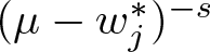 $(\mu-w^{*}_{j})^{-s}$ of function
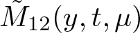 $\tilde{M}_{12}(y,t,\mu)$ is
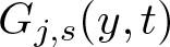 $G_{j,s}(y,t)$. Through the same method, we have
 \begin{align}
\begin{split}
G_{j,s}&=(-1)^{m+1}\frac{i\tilde{\alpha}_{+}(y,t)}{4}D\sum_{l=s}^{N}\sum_{m=0}^{l-s}
\left(\frac{r^{*}_{j,l}\zeta^{*}_{j,l-s-m}}{(w^{*}_{j}-1)^{m+1}}+
\frac{r^{*}_{j,l}\zeta^{*}_{j,l-s-m}}{(w^{*}_{j}+1)^{m+1}}\right)\\
&+\sum_{l=s}^{N}\sum_{m=0}^{l-s}
+\sum_{l=s}^{N}\sum_{m=0}^{l-s}\sum_{p=1}^{2}\sum_{q=1}^{N}
\left(
\begin{array}{c}
q+m-1\\
m \\
\end{array}
\right)\times\\
&r^{*}_{j,l}\zeta^{*}_{j,l-s-m}\left\{\frac{(-1)^{m}}
{(w^{*}_{j}-w_{p})^{q+m}}
+\frac{(-1)^{m+q}}{(w^{*}_{j}+w^{*}_{p})^{q+m}}\right\}F_{p,q},
\end{split}
\end{align}
The system (Equation 2.58) has the following solution For the sake of convenience, selecting the suitable notations for  $j,p=1,2,$
 \begin{align}
|\eta^{1}_{j}\rangle=(\eta^{1}_{j1},\ldots,\eta^{1}_{jN})^{T},\quad
|\eta^{2}_{j}\rangle=(\eta^{2}_{j1},\ldots,\eta^{2}_{jN})^{T},
\end{align}
 \begin{align*}
\eta^{1}_{js}&=\frac{i\tilde{\alpha}_{+}(y,t)}{4}\sum_{l=s}^{N}\sum_{m=0}^{l-s}
\left(\frac{(-1)^{m}}{(w_{j}-1)^{m+1}}-\frac{(-1)^{m}}{(w_{j}+1)^{m+1}} \right)r_{j,l}\zeta_{j,l-s-m},\\
\eta^{2}_{js}&=\sum_{l=s}^{N}\sum_{m=0}^{l-s}r^{*}_{j,l}\zeta^{*}_{j,l-s-m}\\
&-\frac{i\tilde{\alpha}_{+}(y,t)}{4}D\sum_{l=s}^{N}\sum_{m=0}^{l-s}
\left(\frac{(-1)^{m}}{(w^{*}_{j}-1)^{m+1}}+\frac{(-1)^{m}}{(w^{*}_{j}+1)^{m+1}} \right)r^{*}_{j,l}\zeta^{*}_{j,l-s-m},
\end{align*}
then defining the N × N matrices  $\Omega_{j,p}=[\Omega_{j,p}]_{s,q}$ and
 $\tilde{\Omega}_{j,p}=[\tilde{\Omega}_{j,p}]_{s,q}$ for
 $s,q=1,2,\cdots,N$ as follows
 \begin{align}
\begin{split}
\Omega_{j,p}=\sum_{l=s}^{N}\sum_{m=0}^{l-s}
\left(
\begin{array}{c}
q+m-1\\
m \\
\end{array}
\right)
r_{j,l}\zeta_{j,l-s-m}\left\{\frac{(-1)^{m}}{(w_{j}-w^{*}_{p})^{q+m}}
+\frac{(-1)^{m+q+1}}{(w_{j}+w_{p})^{q+m}}\right\},
\end{split}
\end{align}
 \begin{align}
\begin{split}
\tilde{\Omega}_{j,p}=\sum_{l=s}^{N}\sum_{m=0}^{l-s}
\left(
\begin{array}{c}
q+m-1\\
m \\
\end{array}
\right)
r^{*}_{j,l}\zeta^{*}_{j,l-s-m}\left\{\frac{(-1)^{m}}
{(w^{*}_{j}-w_{p})^{q+m}}
+\frac{(-1)^{m+q}}{(w^{*}_{j}+w^{*}_{p})^{q+m}}\right\},
\end{split}
\end{align}
 \begin{align}
|A_{1}\rangle=(|\eta^{1}_{1}\rangle, |\eta^{1}_{2}\rangle)^{T},\quad
|A_{2}\rangle=(-|\eta^{2}_{1}\rangle, -|\eta^{2}_{2}\rangle)^{T},
\end{align}
 \begin{align}
|F_{p}\rangle=(F_{p,1},\ldots,F_{p,N})^{T},\quad
|G_{p}\rangle=(G_{p,1},\ldots,G_{p,N})^{T},
\end{align}
 \begin{align}
\Omega=
\left(\begin{array}{cc}
\Omega_{1,1} & \Omega_{1,2} \\
\Omega_{2,1} & \Omega_{2,2}
\end{array}\right),\quad
\tilde{\Omega}=
\left(\begin{array}{cc}
\tilde{\Omega}_{1,1} & \tilde{\Omega}_{1,2} \\
\tilde{\Omega}_{2,1} & \tilde{\Omega}_{2,2}
\end{array}\right),\quad
I_{\varepsilon}=
\left(\begin{array}{cc}
-I & 0 \\
0 & -I
\end{array}\right),
\end{align}
where I is a N × N identity matrix and the definition of Ω matrix and  $\tilde{\Omega}$ matrix is the same. Combining functions (Equation 3.66)–(Equation 3.68), we have
 \begin{equation}
\begin{aligned}
&I|F_{p}\rangle-\Omega_{j,p}|G_{p}\rangle=|\eta^{1}_{j}\rangle,\\
&\tilde{\Omega}_{j,p}|F_{p}\rangle-I|G_{p}\rangle=-|\eta^{2}_{j}\rangle.
\end{aligned}
\end{equation}
After taking
 \begin{align}
|K_1\rangle=(|F_{1}\rangle,|F_{2}\rangle)^{T},\quad
|K_2\rangle=(|G_{1}\rangle,|G_{2}\rangle)^{T},
\end{align}
by straight calculation, we have
 \begin{align}
\begin{split}
&|K_{1}\rangle=(I_{\varepsilon}+\Omega\tilde{\Omega})^{-1}\Omega|A_{2}\rangle-
(I_{\varepsilon}+\Omega\tilde{\Omega})^{-1}|A_{1}\rangle,\\
&|K_{2}\rangle=-(I_{\varepsilon}+\tilde{\Omega}\Omega)^{-1}\tilde{\Omega}|A_{1}\rangle+
(I_{\varepsilon}+\tilde{\Omega}\Omega)^{-1}|A_{2}\rangle.
\end{split}
\end{align}
The new expression of Equation 3.63a are derived as
 \begin{equation}
\begin{split}
\tilde{M}_{11}
&=1-\frac{i\tilde{\alpha}_{+}(y,t)}{4}D\left(\frac{1}{\mu-1}+\frac{1}{\mu+1}\right)\\
&+\frac{\det(I_{\varepsilon}+\Omega\tilde{\Omega}+\Omega|A_{2}\rangle\langle E(\mu)|)-
\det(I_{\varepsilon}+\Omega\tilde{\Omega}+|A_{1}\rangle\langle E(\mu)|)}
{\det(I_{\varepsilon}+\Omega\tilde{\Omega})},
\end{split}
\end{equation}
 \begin{equation}
\begin{split}
\tilde{M}_{12}&=\frac{i\tilde{\alpha}_{+}(y,t)}{4}\left(\frac{1}{\mu-1}-\frac{1}{\mu+1}\right)\\
&+\frac{\det(I_{\varepsilon}+\tilde{\Omega}\Omega+|A_{2}\rangle\langle\tilde{E}(\mu)|)-
\det(I_{\varepsilon}+\tilde{\Omega}\Omega+\tilde{\Omega}|A_{1}\rangle\langle\tilde{E}(\mu)|)}
{\det(I_{\varepsilon}+\tilde{\Omega}\Omega)},
\end{split}
\end{equation}
with
 \begin{equation}
\begin{split}
&\langle E(\mu)|=(\langle E_{1}(\mu)|,\langle E_{2}(\mu)|),\quad
\langle E_{j}(\mu)|
=(E_{j1},\ldots,E_{jN}),\\
&\langle\tilde{E}(\mu)|=(\langle\tilde{E}_{1}(\mu)|,\langle\tilde{E}_{2}(\mu)|),\quad
\langle\tilde{E}_{j}(\mu)|
=(\tilde{E}_{j1},\ldots,\tilde{E}_{jN}),\\
&\langle E^{\prime}(\mu)|=
(\langle E^{\prime}_{1}(\mu)|,\langle E^{\prime}_{2}(\mu)|),\quad
\langle E^{\prime}_{j}(\mu)|=
(E^{\prime}_{j1},\ldots,E^{\prime}_{jN}),\\
&\langle\tilde{E}^{\prime}(\mu)|
=(\langle\tilde{E}^{\prime}_{1}(\mu)|,\langle\tilde{E}^{\prime}_{2}(\mu)|),\quad
\langle\tilde{E}^{\prime}_{j}(\mu)|=
(\tilde{E}^{\prime}_{j1},\ldots,\tilde{E}^{\prime}_{jN}),
\end{split}
\end{equation}
 \begin{align*}
&E_{js}=\frac{1}{(\mu-w_{j})^{s}}+\frac{(-1)^{s}}{(\mu+w^{*}_{j})^{s}},\quad
\tilde{E}_{js}=\frac{1}{(\mu-w^{*}_{j})^{s}}+\frac{(-1)^{s+1}}{(\mu+w_{j})^{s}},\\
&E^{\prime}_{js}=\frac{-s}{(\mu-w_{j})^{s+1}}+\frac{s(-1)^{s+1}}{(\mu+w^{*}_{j})^{s+1}},\quad
\tilde{E}^{\prime}_{js}=\frac{-s}{(\mu-w^{*}_{j})^{s+1}}+\frac{s(-1)^{s}}{(\mu+w_{j})^{s+1}}.
\end{align*}
According to the symmetry conditions (Equation 3.22), we get that
 \begin{align}
\begin{split}
\tilde{M}_{21}&=-\frac{i\tilde{\alpha}_{+}(y,t)}{4}\left(\frac{1}{\mu-1}-\frac{1}{\mu+1}\right)\\
&+\frac{\det(I_{\varepsilon}+\Omega^{*}\tilde{\Omega}^{*}+|A^{*}_{2}\rangle\langle \tilde{E}^{*}(\mu^{*})|)-
\det(I_{\varepsilon}+\Omega^{*}\tilde{\Omega}^{*}+\tilde{\Omega}^{*}|A^{*}_{1}\rangle\langle \tilde{E}^{*}(\mu^{*})|)}
{\det(I_{\varepsilon}+\Omega^{*}\tilde{\Omega}^{*})}.
\end{split}
\end{align}
Hence the precise expression formula for the solution of cCH equation with single high-order pole under the NZBCs can be obtained in theorem 3.14.
Theorem 3.14
The solution of cCH equation with single high-order pole under the nonzero condition can be derived as the form
 \begin{align}
\hat{u}(x,t)=-2(\tilde{M}^{\prime}_{12}(i)\tilde{M}_{11}(i)
+\tilde{M}^{\prime}_{21}(i)\tilde{M}^{-1}_{11}(i)),
\end{align}
 \begin{align*}
x=x(y,t)=y+2\ln\tilde{M}_{11}(i),
\end{align*}
with
 \begin{align*}
\tilde{M}_{11}(i)&=1-\frac{\tilde{\alpha}_{+}(y,t)D}{4}+
\frac{\det(I_{\varepsilon}+\Omega\tilde{\Omega}+\Omega|A_{2}\rangle\langle E(i)|)-
\det(I_{\varepsilon}+\Omega\tilde{\Omega}+|A_{1}\rangle\langle E(i)|)}{\det(I_{\varepsilon}+\Omega\tilde{\Omega})},\\
\tilde{M}^{\prime}_{12}(i)&=\frac{\tilde{\alpha}_{+}(y,t)}{4}+
\frac{\det(I_{\varepsilon}+\tilde{\Omega}\Omega+|A_{2}\rangle\langle\tilde{E}^{\prime}(i)|)-
\det(I_{\varepsilon}+\tilde{\Omega}\Omega+\tilde{\Omega}|A_{1}\rangle\langle\tilde{E}^{\prime}(i)|)}
{\det(I_{\varepsilon}+\tilde{\Omega}\Omega)},\\
\tilde{M}^{\prime}_{21}(i)& =-\frac{\tilde{\alpha}_{+}(y,t)}{4}\\
&\quad+\frac{\det(I_{\varepsilon}+\Omega^{*}\tilde{\Omega}^{*}+|A^{*}_{2}\rangle\langle \tilde{E}^{\prime*}(-i)|)-
\det(I_{\varepsilon}+\Omega^{*}\tilde{\Omega}^{*}+\tilde{\Omega}^{*}|A^{*}_{1}\rangle\langle \tilde{E}^{\prime*}(-i)|)}
{\det(I_{\varepsilon}+\Omega^{*}\tilde{\Omega}^{*})},
\end{align*}
where D is shown in (Equation 3.21),  $\tilde{\alpha}_{+}(y,t)\in\mathbb{R}$, and the elements
 $|A_{1}\rangle$,
 $|A_{2}\rangle$, Iɛ, Ω,
 $\tilde{\Omega}$,
 $\langle E(i)|$,
 $\langle\tilde{E}(i)|$,
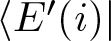 $\langle E^{\prime}(i)|$,
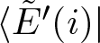 $\langle \tilde{E}^{\prime}(i)|$ are defined in (Equation 3.72), (Equation 3.74), and (Equation 3.80).
3.3.1. One-soliton solution
Next, to construct the simple one-soliton solution of cCH equation under NZBCs, we consider the specific data as follows.
Case 4: For this case, we consider the situation N = 1, Assuming  $w_{1}=z_{0}=e^{i\lambda}\in\mathbb{C}^{+}$,
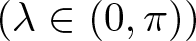 $(\lambda\in(0,\pi))$ is one-order pole of scattering data
 $a(\mu)$, then we have
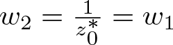 $w_{2}=\frac{1}{z^{*}_{0}}=w_{1}$. It can be obtained that
 $\theta(e^{i\lambda})=\theta(-e^{-i\lambda})$. Next we define
 $\theta_{1}\triangleq\theta(e^{i\lambda})=\frac{i\sin\lambda y}{2t}-\frac{2i\sin\lambda}{\cos^{2}\lambda}$, hence
 $e^{2it\theta_{2}}$ is real. Suppose that D = 1,
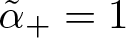 $\tilde{\alpha}_{+}=1$,
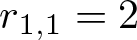 $r_{1,1}=2$,
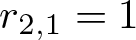 $r_{2,1}=1$. Then the parameters satisfy the following relationships, there
 $\Omega_{1,1}=\Omega_{1,2}=\Omega_{2,1}=\Omega_{2,2}$,
 $\tilde{\Omega}_{1,1}=\tilde{\Omega}_{1,2}=\tilde{\Omega}_{2,1}=\tilde{\Omega}_{2,2}$,
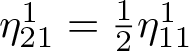 $\eta^{1}_{21}=\frac{1}{2}\eta^{1}_{11}$,
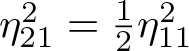 $\eta^{2}_{21}=\frac{1}{2}\eta^{2}_{11}$,
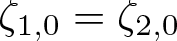 $\zeta_{1,0}=\zeta_{2,0}$.
 \begin{align*}
\zeta_{1,0}=e^{-\frac{4\sin\lambda}{\cos^{2}\lambda e^{2i\lambda}}\left(\left(t+\frac{y}{8}\right)e^{2i\lambda}+\frac{y}{16}(e^{4i\lambda}+1)\right)},
\end{align*}
 \begin{align*}
\Omega_{1,1}=2e^{-\frac{4\sin\lambda}{\cos^{2}\lambda e^{2i\lambda}}\left(\left(t+\frac{y}{8}\right)e^{2i\lambda}+\frac{y}{16}(e^{4i\lambda}+1)\right)}
\left(\frac{1}{e^{i\lambda}-e^{-i\lambda}+\frac{1}{2e^{i\lambda}}}\right),
\end{align*}
 \begin{align*}
\tilde{\Omega}_{1,1}=2e^{-\frac{((16t+2y)e^{-2i\lambda}+y(e^{-4i\lambda}+1))\sin\lambda}{4\cos^{2}\lambda e^{2i\lambda}}}\left(\frac{1}{e^{-i\lambda}-e^{i\lambda}-\frac{1}{2e^{-i\lambda}}}\right),
\end{align*}
 \begin{align*}
\eta^{1}_{11}=\frac{i}{2}\left(\frac{1}{e^{i\lambda}-1}-\frac{1}{e^{i\lambda}+1}\right)
e^{-\frac{4\sin\lambda}{\cos^{2}\lambda e^{2i\lambda}}\left(\left(t+\frac{y}{8}\right)e^{2i\lambda}+\frac{y}{16}(e^{4i\lambda}+1)\right)},
\end{align*}
 \begin{align*}
\eta^{2}_{11}=\left(2-\frac{i}{2}\left(\frac{1}{e^{i\lambda}-1}+\frac{1}{e^{i\lambda}+1}\right)\right)e^{-\frac{4\sin\lambda}{\cos^{2}\lambda e^{2i\lambda}}\left(\left(t+\frac{y}{8}\right)e^{2i\lambda}+\frac{y}{16}(e^{4i\lambda}+1)\right)},
\end{align*}
substituting the above results into the formula (Equation 3.82) we can obtain the one-soliton solution of cCH equation under NZBCs.
Supposing 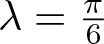 $\lambda=\frac{\pi}{6}$, the expression for the solution is
 \begin{align}
\hat{u}(x,t)=-2\left(T^{1}_{2}T^{1}_{1}+\frac{T^{1}_{3}}{T^{1}_{1}}\right),
\end{align}
 \begin{align*}
x=x(y,t)=y+2\ln T^{1}_{1},
\end{align*}
 \begin{align*}
T^{1}_{1}=\frac{12ie^{-\frac{8t}{3}-\frac{y}{2}}+153i\sqrt{3}e^{-\frac{16t}{3}-y}+20i\sqrt{3}-246e^{-\frac{16t}{3}-y}-20}
{(i\sqrt{3}-1)\left(27e^{-\frac{16t}{3}-\frac{y}{2}}+18ie^{-\frac{16t}{3}-\frac{y}{2}}\sqrt{3}+4\right)},
\end{align*}
 \begin{align*}
T^{1}_{2}=\frac{141ie^{-\frac{16t}{3}-\frac{y}{2}}\sqrt{3}-6e^{-\frac{8t}{3}-\frac{y}{2}}+216e^{-\frac{16t}{3}-\frac{y}{2}}+32}
{27e^{-\frac{16t}{3}-\frac{y}{2}}+18ie^{-\frac{16t}{3}-\frac{y}{2}}\sqrt{3}+4},
\end{align*}
 \begin{align*}
T^{1}_{3}=-\frac{18(i\sqrt{3}-1)e^{-\frac{8t}{3}-\frac{y}{2}}-(351i\sqrt{3}+189)e^{-\frac{16t}{3}-\frac{y}{2}}-32i\sqrt{3}+32}
{(i\sqrt{3}-1)\left(18ie^{-\frac{16t}{3}-\frac{y}{2}}-27e^{-\frac{16t}{3}-\frac{y}{2}}-4\right)}.
\end{align*}
In accordance with the construction process of the RH problem, it can be known that there are singularities 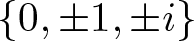 $\left\{0,\pm1,\pm i\right\}$ of the spectral parameter z. Since we choose
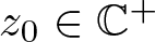 $z_{0}\in\mathbb{C}^{+}$ here and
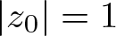 $|z_{0}|=1$,
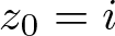 $z_{0}=i$ is the singularity of solution
 $\hat{u}$. From the propagation of waves in figure 7, the bright soliton solution is the hump-kink interacted solution. Based on the intensity distribution figure captured at various time points, when the wave peaks and then drops a certain height, it continues to propagate but does not return to the same height as before.
(a)–(c) describe the local structure, density, and intensity profiles with different times of one-soliton solution  $|u|$. Parameters
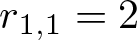 $r_{1,1}=2$,
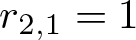 $r_{2,1}=1$,
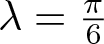 $\lambda=\frac{\pi}{6}$.

Figure 7 Long description
Three plots labeled (a), (b) and (c) show different aspects of a one-soliton solution at different times. Image (a) is a three-dimensional surface plot showing the local structure. The horizontal plane axes are labeled x and t and the vertical axis represents the amplitude of the solution. The surface shows a single sharp peak rising from a near-flat base, with the peak located near the center of the plotted domain. The x-axis and t-axis each span from approximately negative 5 to positive 5. Image (b) is a two-dimensional density plot. The horizontal axis represents x, spanning from approximately negative 10 to positive 10. The vertical axis represents t, also spanning from approximately negative 10 to positive 10. The density scale runs from low to high values. A narrow near-vertical bright band is visible near x equals 0, running along the full extent of the t-axis. The surrounding region shows uniformly low density values. This band indicates the spatial concentration of the soliton across all time values shown. Image (c) is a line plot showing intensity profiles. The horizontal axis represents x, spanning from approximately negative 10 to positive 10. The vertical axis represents intensity, spanning from 0 upward. Three curves are plotted, each corresponding to a different time value. All three curves show a single peak centered near x equals 0. The tallest and narrowest peak reaches approximately 1.0 on the vertical axis. The second curve shows a peak of moderate height, slightly lower than the first. The third curve shows the broadest and lowest peak among the three. The three peaks are all located near x equals 0, with no visible lateral shift between them.
Supposing 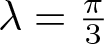 $\lambda=\frac{\pi}{3}$, the solution can be obtained as follows
 \begin{align}
\hat{u}(x,t)=-2\left(T^{2}_{2}T^{2}_{1}+\frac{T^{2}_{3}}{T^{2}_{1}}\right),
\end{align}
 \begin{align*}
x=x(y,t)=y+2\ln T^{2}_{1},
\end{align*}
 \begin{align*}
T^{2}_{1}=&\frac{1}{\varpi^{2}_{1}}\left((5520-696i+(1080-816i)\sqrt{3})e^{(-16t-y)\sqrt{3}}\right)+\\
&\frac{1}{\varpi^{2}_{1}}\left(320e^{-\frac{\sqrt{3}(16t+y)}{2}}\sqrt{3}+64-96i+(64i-32)\sqrt{3}\right),
\end{align*}
 \begin{align*}
T^{2}_{2}=&\frac{1}{\varpi^{2}_{2}}\left((-1056-1728i-(192+1248i)\sqrt{3})e^{(-16t-y)\sqrt{3}}+896-1536i+512\sqrt{3}\right)+\\
&\frac{1}{\varpi^{2}_{2}}\left((-15360+28800i+(-9600+15360i)\sqrt{3})e^{-\frac{\sqrt{3}(16t+y)}{2}}-896i\sqrt{3}\right),
\end{align*}
 \begin{align*}
T^{2}_{3}=&\frac{1}{\varpi^{2}_{3}}\left((1056+1728i-(192+1248i)\sqrt{3})e^{(-16t-y)\sqrt{3}}-896+1536i+512\sqrt{3}\right)+\\
&\frac{1}{\varpi^{2}_{3}}\left((-7680+17280i+(5760-7680i)\sqrt{3})e^{-\frac{\sqrt{3}(16t+y)}{2}}-896i\sqrt{3}\right),
\end{align*}
 \begin{align*}
\varpi^{2}_{1}&=80(1+i\sqrt{3})(2-\sqrt{3})((3+6i\sqrt{3})e^{(-16t-y)\sqrt{3}})+4,\\
\varpi^{2}_{2}&=-40(3+2\sqrt{3})(i\sqrt{3}-1)((3+6i)e^{-\frac{\sqrt{3}(16t+y)}{2}}+4),\\
\varpi^{2}_{3}&=-320(2-\sqrt{3})^{2}(i\sqrt{3}+1)((6i\sqrt{3}-3)e^{-\frac{\sqrt{3}(16t+y)}{2}}-4).
\end{align*}
From figure 8, it can be seen that the peak of soliton does not immediately propagate smoothly when it falls from the highest point but rather fluctuates and appears as a smaller peak.
(a)–(c) describe the local structure, density, and intensity profiles with different times of one-soliton solutions  $|u|$. Parameters
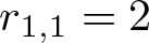 $r_{1,1}=2$,
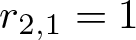 $r_{2,1}=1$,
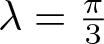 $\lambda=\frac{\pi}{3}$.

Figure 8 Long description
Three plots together show the local structure, density and intensity profiles of one-soliton solutions at different times. Plot (a) is a three-dimensional surface plot. The horizontal axes each range from negative 10 to positive 10. The vertical axis represents the amplitude or height of the soliton. A single narrow ridge runs diagonally across the surface, indicating a localized soliton peak. The ridge remains concentrated in a narrow band. Plot (b) is a two-dimensional density plot. The horizontal axis ranges from negative 4 to positive 4 and the vertical axis ranges from negative 4 to positive 4. A narrow vertical band of high density runs through the center of the plot. The surrounding regions show low density. A color scale on the right side of the plot ranges from low values at the bottom to high values at the top, encoding the density magnitude. Plot (c) is a line plot with three curves, each corresponding to a different time point as identified in the legend. The horizontal axis ranges from approximately negative 30 to positive 30. The vertical axis ranges from approximately negative 1 to positive 3. All three curves show a sharp peak near the center of the horizontal axis. The tallest peak reaches approximately 3 on the vertical axis and is narrow. A secondary smaller peak appears to the right of the main peak for at least one curve. The remaining portions of all three curves stay near zero. The three curves differ in their peak heights and the presence or position of the secondary peak, indicating how the soliton intensity profile changes over time.
3.3.2. Two-order pole solution
In an effort to construct the two-order pole solution of cCH equation under NZBCs, we consider the specific data as follows. This is for N = 2 case, and the expression of 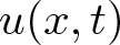 $u(x,t)$ defined in theorem 3.14.
Case 5: Assuming that  $w_{1}=z_{0}=e^{i\lambda}\in\mathbb{C}^{+}$ be the two-order zero point of the scattering data
 $a(\mu)$, then
 $w_{2}=w_{1}$ is also the two-order zero point of
 $a(\mu)$. The discrete spectrum is the set
 $\mathcal{X}=\left\{e^{i\lambda}, -e^{-i\lambda}, e^{-i\lambda}, -e^{i\lambda}\right\}$. For the purpose of displaying characteristics of soliton propagations more clearly, we select some appropriate parameters to construct the two-order pole solutions of cCH equation. The dynamic behaviours of solitons are shown in Figures (9)–(10).
(a)–(c) describe the local structure, density, and intensity profiles with different times of the soliton solutions  $|u|$ with one two-order pole. Parameters
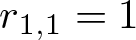 $r_{1,1}=1$,
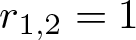 $r_{1,2}=1$,
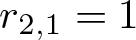 $r_{2,1}=1$,
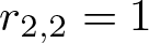 $r_{2,2}=1$,
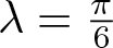 $\lambda=\frac{\pi}{6}$.

Figure 9 Long description
Three panels labeled (a), (b) and (c) present soliton solution profiles with one two-order pole across spatial variable x and time variable t. Panel (a) is a 3D surface plot. The x-axis is labeled x, units not shown and the y-axis is labeled t, units not shown. The z-axis is labeled with an intensity-related quantity, units not shown. A narrow, sharply peaked ridge rises steeply along a diagonal path across the x-t plane. The ridge is concentrated within a narrow band, indicating a localized soliton structure. The surface is flat and near zero away from this ridge. Panel (b) is a 2D heatmap or colormap plot of density over the x-t plane. The x-axis is labeled x, units not shown, ranging approximately from minus 20 to 30. The y-axis is labeled t, units not shown, ranging approximately from minus 20 to 20. A dominant diagonal band runs from lower left to upper right across the plot, flanked by narrower secondary bands. The central band occupies a wider region compared to the surrounding bands. The density values transition sharply across band boundaries. Panel (c) is an overlaid line plot showing intensity profiles. The x-axis is labeled t, units not shown, ranging approximately from minus 3 to 3. The y-axis is labeled with an intensity quantity, units not shown. Multiple curves are plotted together, each corresponding to a different value of x or a different time slice. The curves share a common baseline near zero and each rises to a distinct sharp peak near t equals 0. The peaks are narrow and closely spaced. Individual curves are distinguishable by line style, though legend labels are not clearly readable at this resolution.
(a)–(c) describe the local structure, density, and intensity profiles with different times of the soliton solutions  $|u|$ with one two-order pole. Parameters
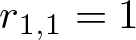 $r_{1,1}=1$,
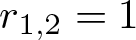 $r_{1,2}=1$,
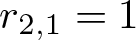 $r_{2,1}=1$,
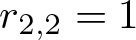 $r_{2,2}=1$,
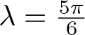 $\lambda=\frac{5\pi}{6}$.

Figure 10 Long description
Three panels labeled a, b and c, each depicting soliton solutions with one two-order pole at different times. Panel a is a 3D surface plot. The x-axis is labeled x, units not shown and the y-axis is labeled t, units not shown. The z-axis represents the amplitude of the soliton solution, units not shown. The surface displays a sharp ridge running diagonally across the plot, indicating the soliton position shifts as time increases. The ridge rises steeply from a near-flat base to a prominent peak, with the surrounding surface remaining close to zero. Panel b is a 2D density plot. The x-axis is labeled x, ranging approximately from minus 30 to 30, units not shown. The y-axis is labeled t, ranging approximately from minus 30 to 30, units not shown. The plot shows color-coded intensity values across the x-t plane. A narrow diagonal band runs from the lower-left region toward the upper-right region, representing the soliton trajectory. The surrounding regions display near-uniform low-intensity values. Transition boundaries between regions are sharp and clearly defined. Panel c is a line plot showing intensity profiles at different values of time t. The x-axis is labeled x, units not shown. The y-axis is labeled intensity, units not shown. Multiple curves are present, each corresponding to a distinct value of t. A dominant narrow peak is visible near x equals 0, with the peak height substantially larger than the surrounding profile. Smaller secondary peaks appear symmetrically on either side of the central peak. The curves differ in peak height and width across the plotted time values. No legend labels are visible to individually identify each curve; multiple distinct curves are shown without textual labels.
Setting 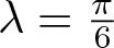 $\lambda=\frac{\pi}{6}$,
 $\left\{r_{1,1}=1, r_{1,2}=1, r_{2,1}=1, r_{2,2}=1\right\}$, D = 1,
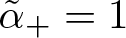 $\tilde{\alpha}_{+}=1$. Besides,
 $\Omega_{1,1}=\Omega_{1,3}=\Omega_{3,1}=\Omega_{3,3}$,
 $\Omega_{1,2}=\Omega_{1,4}=\Omega_{3,2}=\Omega_{3,4}$,
 $\Omega_{2,1}=\Omega_{2,3}=\Omega_{4,1}=\Omega_{4,3}$,
 $\Omega_{2,2}=\Omega_{2,4}=\Omega_{4,2}=\Omega_{4,4}$,
 $\tilde{\Omega}_{1,1}=\tilde{\Omega}_{1,3}=\tilde{\Omega}_{3,1}=\tilde{\Omega}_{3,3}$,
 $\tilde{\Omega}_{1,2}=\tilde{\Omega}_{1,4}=\tilde{\Omega}_{3,2}=\tilde{\Omega}_{3,4}$,
 $\tilde{\Omega}_{2,1}=\tilde{\Omega}_{2,3}=\tilde{\Omega}_{4,1}=\tilde{\Omega}_{4,3}$,
 $\tilde{\Omega}_{2,2}=\tilde{\Omega}_{2,4}=\tilde{\Omega}_{4,2}=\tilde{\Omega}_{4,4}$. In view of the construction process for simple high-order pole solutions under NZBCs and the parameter expressions of obtained solutions in theorem 3.14, we further obtain
 \begin{align*}
\zeta_{1,0}=\zeta_{2,0}=e^{-\frac{2t}{3}-\frac{y}{2}},
\end{align*}
 \begin{align*}
\zeta_{1,1}=\zeta_{2,1}=\frac{8i(20t+9y)e^{-\frac{2t}{3}-\frac{y}{2}}(i\sqrt{3}-1)}
{(i\sqrt{3}+3)^3(\sqrt{3}+i)^2},
\end{align*}
 \begin{align*}
\Omega_{1,1}=\frac{5\sqrt{3}}{18}\left(\left(-\frac{21+27y}{20}+\frac{3i}{2}-3t\right)\sqrt{3}
+it+\frac{9i(y-1)}{20}-\frac{9}{10}\right)e^{-\frac{2t}{3}-\frac{y}{2}},
\end{align*}
 \begin{align*}
\Omega_{1,2}=\frac{1440e^{-\frac{2t}{3}-\frac{y}{2}}}{(i\sqrt{3}+3)^3(\sqrt{3}+i)^4}
\left(\sqrt{3}\left(\frac{y-6}{20}+\frac{i}{10}+\frac{t}{9}\right)+it+\frac{9i(y+1)}{20}+\frac{1}{2}\right),
\end{align*}
 \begin{align*}
\Omega_{2,1}=-\frac{e^{-\frac{2t}{3}-\frac{y}{2}}(-2+i\sqrt{3})}{\sqrt{3}+i},\quad
\Omega_{2,2}=\frac{e^{-\frac{2t}{3}-\frac{y}{2}}(-3-2i\sqrt{3})}{(\sqrt{3}+i)^2},
\end{align*}
 \begin{align*}
\tilde{\Omega}_{1,1}=\frac{1}{24}\left((-6+3i+20it+9iy)\sqrt{3}+27+18i+20t+9y\right)
e^{-\frac{2t}{3}-\frac{y}{2}},
\end{align*}
 \begin{align*}
\tilde{\Omega}_{1,2}=\frac{1120\left(\left(\frac{3}{10}+\frac{3i}{14}+\frac{t}{7}+\frac{9y}{140}\right)\sqrt{3}
+it+\frac{9iy}{20}-\frac{27}{70}+\frac{9i}{10}\right)e^{-\frac{2t}{3}-\frac{y}{2}}}{(i\sqrt{3}-3)^3(i-\sqrt{3})^4},
\end{align*}
 \begin{align*}
\tilde{\Omega}_{2,1}=\frac{-i\sqrt{3}e^{-\frac{2t}{3}-\frac{y}{2}}}{i-\sqrt{3}},\quad
\tilde{\Omega}_{2,2}=\frac{(2i\sqrt{3}-1)e^{-\frac{2t}{3}-\frac{y}{2}}}{(i-\sqrt{3})^2},
\end{align*}
 \begin{align*}
\eta^{1}_{11}=\eta^{1}_{21}=\frac{-1280i\left(\left(-\frac{6}{5}+\frac{3i}{5}-t-\frac{9y}{20}\right)
\sqrt{3}+it+\frac{9iy}{20}\right)e^{-\frac{2t}{3}-\frac{y}{2}}}
{4(i\sqrt{3}-1)^2(i\sqrt{3}+3)^3(\sqrt{3}+i)^2},
\end{align*}
 \begin{align*}
\eta^{2}_{11}=\eta^{2}_{21}=\frac{(-1920i\sqrt{3}-7680it-3456iy+5760-2304i)e^{-\frac{2t}{3}-\frac{y}{2}}}
{4(i\sqrt{3}+1)^2(i\sqrt{3}-3)^3(i-\sqrt{3})^2},
\end{align*}
 \begin{align*}
\eta^{1}_{12}=\eta^{1}_{22}=\frac{ie^{-\frac{2t}{3}-\frac{y}{2}}}{i\sqrt{3}-1},\quad
\eta^{2}_{12}=\eta^{2}_{22}=-\frac{3e^{-\frac{2t}{3}-\frac{y}{2}}}{2},
\end{align*}
then substituting the above results into the expression of solution (Equation 3.82), we can obtain the two-order pole solution of cCH equation, Figure 9 shows the dynamic behaviour of soliton propagation, with three images presenting the local structure, density, and intensity profiles at different times of two-order pole solutions with the above parameters.
In addition, we select parameter 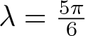 $\lambda=\frac{5\pi}{6}$ and use the same process to obtain the dynamic propagation of the solution shown in Figure 10. From these two Figures 9–10, it can be seen that when the two waves collide at the centre, a larger peak is generated, and then they continue to propagate along the previous trajectory, but the energy decreases.
3.4. Multiple high-order pole solutions
The general circumstance that scattering data  $a(\mu)$ has N high-order poles
 $z_{1},z_{2},\cdots,z_{N}$ will be considered, there
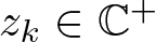 $z_{k}\in\mathbb{C}^{+}$ for all
 $k=1,2,\ldots,N$, and their powers are
 $n_{1},n_{2},\ldots,n_{N}$, respectively. Let
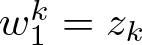 $w^{k}_{1}=z_{k}$ and
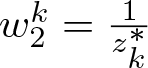 $w^{k}_{2}=\frac{1}{z^{*}_{k}}$,
 $k=1,2,\ldots,N$, just like the case of one high-order pole, from the definition of
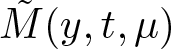 $\tilde{M}(y,t,\mu)$, it can be seen that
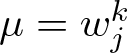 $\mu=w^{k}_{j}$ and
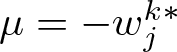 $\mu=-w^{k*}_{j}$
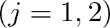 $(j=1,2)$ are N-order pole points of
 $\tilde{M}_{11}$. Simultaneously,
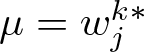 $\mu=w^{k*}_{j}$ and
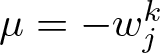 $\mu=-w^{k}_{j}$
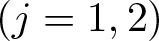 $(j=1,2)$ are N-order pole points of
 $\tilde{M}_{12}$.
Under the assumption that 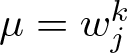 $\mu=w^{k}_{j}$
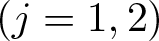 $(j=1,2)$ are nk-order zero points of
 $a(\mu)$ for
 $k=1,2,\ldots,N$, by the Wronskian
 $a(\mu)=Wr(\check{\phi}_{-1},\check{\phi}_{+2})$, there exist complex constants
 $b^{k}_{j,s}$
 $(s=1,2,\ldots,n_N)$ satisfy the follows
 \begin{equation}
\frac{\partial^{m}[\check{\phi}_+(y,t,w^{k}_{j})]_{2}}{\partial\mu^{m}}=\sum^{m}_{l=0}\left(\begin{array}{c}
m \\
l
\end{array}\right)
b^{k}_{j,m-l+1}\frac{\partial^{l}[\check{\phi}_-(y,t,w^{k}_{j})]_{1}}{\partial\mu^{l}},
\end{equation}
and
 \begin{equation}
\frac{\partial^{m}[\check{\psi}_+(y,t,w^{k}_{j})]_{2}}{\partial\mu^{m}}=\sum^{m}_{l=0}\left(\begin{array}{c}
m \\
l
\end{array}\right)
b^{k}_{j,m-l+1}\frac{\partial^{l}[\check{\psi}_-(y,t,w^{k}_{j})]_{1}e^{2it\theta(w^{k}_{j})}}{\partial\mu^{l}},
\end{equation}
with  $m=0,1,\ldots,n_{N-1}$. Utilizing the parallel approach in above, we define the
 $n_k\times n_k$ matrices
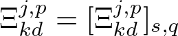 $\Xi^{j,p}_{kd}=[\Xi^{j,p}_{kd}]_{s,q}$ and
 $\tilde{\Xi}^{j,p}_{kd}=[\tilde{\Xi}^{j,p}_{kd}]_{s,q}$ for
 $s,q=1,2,\ldots,n_{k}$ and introduce the following notations for
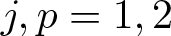 $j,p=1,2$
 \begin{align}
&|\eta^{1k}_{j}\rangle=(\eta^{1k}_{j1},\cdots,\eta^{1k}_{jN})^{T},\quad
|\eta^{2k}_{j}\rangle=(\eta^{2k}_{j1},\cdots,\eta^{2k}_{jN})^{T},
\end{align}
 \begin{align*}
\eta^{1k}_{js}=\frac{i\tilde{\alpha}_{+}(y,t)}{4}\sum_{l=s}^{n_{k}}\sum_{m=0}^{l-s}
\left(\frac{(-1)^{m}}{(w^{k}_{j}-1)^{m+1}}-\frac{(-1)^{m}}{(w^{k}_{j}+1)^{m+1}} \right)r^{k}_{j,l}\zeta^{k}_{j,l-s-m},
\end{align*}
 \begin{align*}
\eta^{2k}_{js}&=\sum_{l=s}^{n_{k}}\sum_{m=0}^{l-s}r^{k*}_{j,l}\zeta^{k*}_{j,l-s-m}\\
&-\frac{i\tilde{\alpha}_{+}(y,t)}{4}D\sum_{l=s}^{n_{k}}\sum_{m=0}^{l-s}
\left(\frac{(-1)^{m}}{(w^{k*}_{j}-1)^{m+1}}+\frac{(-1)^{m}}{(w^{k*}_{j}+1)^{m+1}} \right)r^{k*}_{j,l}\zeta^{k*}_{j,l-s-m},
\end{align*}
 \begin{align}
r^{k}_{j,l}=\lim_{\mu\rightarrow w^{k}_{j}}\frac{b^{k}_{j,l}}{(n_{k}-l)!}\frac{\partial^{n_{k}-l}}{\partial(\mu-w^{k}_{j})^{n_{k}-l}}
\frac{(\mu-w^{k}_{j})^{n_{k}}}{a(\mu)},
\end{align}
 \begin{align}
\begin{split}
&|B_{1}\rangle=(|A^{1}_{1}\rangle, |A^{2}_{1}\rangle, \cdots, |A^{N}_{1}\rangle)^{T},\quad
|A^{k}_{1}\rangle=(|\eta^{1k}_{1}\rangle, |\eta^{1k}_{2}\rangle)^{T},\\
&|B_{2}\rangle=(|A^{1}_{2}\rangle, |A^{2}_{2}\rangle, \cdots, |A^{N}_{2}\rangle)^{T},\quad
|A^{k}_{2}\rangle=(-|\eta^{2k}_{1}\rangle, -|\eta^{2k}_{2}\rangle)^{T},
\end{split}
\end{align}
 \begin{align}
\begin{split}
\Xi^{j,p}_{k,d}=\sum_{l=s}^{n_{k}}\sum_{m=0}^{l-s}
\left(
\begin{array}{c}
q+m-1\\
m \\
\end{array}
\right)
r^{k}_{j,l}\zeta^{k}_{j,l-s-m}\left\{\frac{(-1)^{m}}{(w^{k}_{j}-w^{k*}_{p})^{q+m}}
+\frac{(-1)^{m+q+1}}{(w^{k}_{j}+w^{k}_{p})^{q+m}}\right\},
\end{split}
\end{align}
 \begin{align}
\begin{split}
\tilde{\Xi}^{j,p}_{k,d}=\sum_{l=s}^{n_{k}}\sum_{m=0}^{l-s}
\left(
\begin{array}{c}
q+m-1\\
m \\
\end{array}
\right)
r^{k*}_{j,l}\zeta^{k*}_{j,l-s-m}\left\{\frac{(-1)^{m}}
{(w^{k*}_{j}-w^{k}_{p})^{q+m}}
+\frac{(-1)^{m+q}}{(w^{k*}_{j}+w^{k*}_{p})^{q+m}}\right\},
\end{split}
\end{align}
 \begin{align}
\Xi=
\begin{pmatrix}
[\Xi^{j,p}_{11}] & \cdots & [\Xi^{j,p}_{1N}] \\
\vdots & \ddots & \vdots \\
[\Xi^{j,p}_{N1}] & \cdots & [\Xi^{j,p}_{NN}] \\
\end{pmatrix},\quad
\tilde{\Xi}=
\begin{pmatrix}
[\tilde{\Xi}^{j,p}_{11}] & \cdots & [\tilde{\Xi}^{j,p}_{1N}] \\
\vdots & \ddots & \vdots \\
[\tilde{\Xi}^{j,p}_{N1}] & \cdots & [\tilde{\Xi}^{j,p}_{NN}] \\
\end{pmatrix},
\end{align}
 \begin{align}
I_{\delta}=
\begin{pmatrix}
I_{\delta_{1}} & & \\
& \ddots & \\
& & I_{\delta_{N}} \\
\end{pmatrix},\quad
I_{\delta_{k}}=
\begin{pmatrix}
-I & \\
& -I \\
\end{pmatrix}_{2n_{k}\times2n_{k}} k=1,\ldots,N,
\end{align}
 \begin{equation}
\begin{split}
&\langle \Lambda(\mu)|=(\langle \Lambda^{1}_{1}(\mu)|,\langle \Lambda^{1}_{2}(\mu)|,\ldots,\langle \Lambda^{N}_{1}(\mu)|,\langle \Lambda^{N}_{2}(\mu)|),\\
&\langle \tilde{\Lambda}(\mu)|=(\langle \tilde{\Lambda}^{1}_{1}(\mu)|,\langle \tilde{\Lambda}^{1}_{2}(\mu)|,\ldots,\langle \tilde{\Lambda}^{N}_{1}(\mu)|,\langle \tilde{\Lambda}^{N}_{2}(\mu)|),\\
&\langle \Lambda^{\prime}(\mu)|=(\langle \Lambda^{1\prime}_{1}(\mu)|,\langle \Lambda^{1\prime}_{2}(\mu)|,\ldots,\langle \Lambda^{N\prime}_{1}(\mu)|,\langle \Lambda^{N\prime}_{2}(\mu)|),\\
&\langle \tilde{\Lambda}^{\prime}(\mu)|=(\langle \tilde{\Lambda}^{1\prime}_{1}(\mu)|,\langle \tilde{\Lambda}^{1\prime}_{2}(\mu)|,\ldots,\langle \tilde{\Lambda}^{N\prime}_{1}(\mu)|,\langle \tilde{\Lambda}^{N\prime}_{2}(\mu)|),
\end{split}
\end{equation}
with
 \begin{align*}
&\langle\Lambda^{k}_{j}(\mu)|=(\Lambda^{k}_{j1},\ldots,\Lambda^{k}_{jn_k}),\quad
\Lambda^{k}_{js}=\frac{1}{(\mu-w^{k}_{j})^{s}}+\frac{(-1)^{s}}{(\mu+w^{k*}_{j})^{s}},\\
&\langle\tilde{\Lambda}^{k}_{j}(\mu)|=(\tilde{\Lambda}^{k}_{j1},\ldots,\tilde{\Lambda}^{k}_{jn_k}),\quad
\tilde{\Lambda}^{k}_{js}=\frac{1}{(\mu-w^{k*}_{j})^{s}}+\frac{(-1)^{s+1}}{(\mu+w^{k}_{j})^{s}},\\
&\langle\Lambda^{k\prime}_{j}(\mu)|=(\Lambda^{k\prime}_{j1},\ldots,\Lambda^{k\prime}_{jn_k}),\quad
\Lambda^{k\prime}_{js}=\frac{-s}{(\mu-w^{k}_{j})^{s+1}}+\frac{s(-1)^{s+1}}{(\mu+w^{k*}_{j})^{s+1}},\\
&\langle\tilde{\Lambda}^{k\prime}_{j}(\mu)|=(\tilde{\Lambda}^{k\prime}_{j1},\ldots,\tilde{\Lambda}^{k\prime}_{jn_k}),\quad
\tilde{\Lambda}^{k\prime}_{js}=\frac{-s}{(\mu-w^{k*}_{j})^{s+1}}+\frac{s(-1)^{s}}{(\mu+w^{k}_{j})^{s+1}}.
\end{align*}
Similar to theorem 3.14, we give the solution of cCH equation with multiple high-order poles as follows.
Theorem 3.15
The multiple high-order pole solutions of cCH equation under the nonzero condition can be obtained as follows
 \begin{align}
\hat{u}(x,t)=-2(\tilde{M}^{\prime}_{12}(i)\tilde{M}_{11}(i)
+\tilde{M}^{\prime}_{21}(i)\tilde{M}^{-1}_{11}(i)),
\end{align}
 \begin{align*}
x=x(y,t)=y+2\ln\tilde{M}_{11}(i),
\end{align*}
with
 \begin{align*}
\tilde{M}_{11}(i)& =1-\frac{\tilde{\alpha}_{+}(y,t)D}{4}+
\frac{\det(I_{\delta}+\Xi\tilde{\Xi}+\Xi|B_{2}\rangle\langle\Lambda(i)|)-
\det(I_{\delta}+\Xi\tilde{\Xi}+|B_{1}\rangle\langle\Lambda(i)|)}{\det(I_{\delta}+\Xi\tilde{\Xi})},\\
\tilde{M}^{\prime}_{12}(i)& =\frac{\tilde{\alpha}_{+}(y,t)}{4}+
\frac{\det(I_{\delta}+\tilde{\Xi}\Xi+|B_{2}\rangle\langle\tilde{\Lambda}^{\prime}(i)|)-
\det(I_{\delta}+\tilde{\Xi}\Xi+\tilde{\Xi}|B_{1}\rangle\langle\tilde{\Lambda}^{\prime}(i)|)}
{\det(I_{\delta}+\tilde{\Xi}\Xi)},\\
\tilde{M}^{\prime}_{21}(i)& =-\frac{\tilde{\alpha}_{+}(y,t)}{4}\\
& \quad +\frac{\det(I_{\delta}+\Xi^{*}\tilde{\Xi}^{*}+|\Lambda^{*}_{2}\rangle\langle \tilde{\Lambda}^{\prime*}(-i)|)-
\det(I_{\delta}+\Xi^{*}\tilde{\Xi}^{*}+\tilde{\Xi}^{*}|\Lambda^{*}_{1}\rangle\langle \tilde{\Lambda}^{\prime*}(-i)|)}
{\det(I_{\delta}+\Xi^{*}\tilde{\Xi}^{*})},
\end{align*}
where D is shown in (Equation 3.21),  $\tilde{\alpha}_{+}(y,t)\in\mathbb{R}$, the elements
 $|B_{1}\rangle$,
 $|B_{2}\rangle$, Iδ, Ξ,
 $\tilde{\Xi}$,
 $\langle\Lambda(i)|$,
 $\langle\tilde{\Lambda}(i)|$,
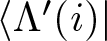 $\langle \Lambda^{\prime}(i)|$, and
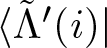 $\langle \tilde{\Lambda}^{\prime}(i)|$ are defined in (Equation 3.89), (Equation 3.92), (Equation 3.93), and (Equation 3.94).
4. Conclusions
In summary, we have studied the multiple high-order pole solutions of the cCH equation with a linear dispersion term by the RH method with ZBCs and NZBCs. In comparison to the previous work presented in reference [Reference Wang and Qiao43], we not only provide the multi-soliton solutions for this equation but also examine the multiple high-order pole solutions in the context of both boundary conditions.
Under ZBCs, in the direct scattering part, we make spectral analysis to the Lax pair. To address the issue of the multi-value problem arising from square roots, a uniformization variable µ is introduced, which leads to the Lax matrices U and V have singularities at the points µ = 0, 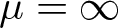 $\mu=\infty$, and the branch cut points
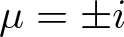 $\mu=\pm i$ in the extended complex µ-plane. In order to control the behaviour of the eigenfunctions at these singular points, we introduce the suitable gauge transformations. This method has been developed by Boutet de Monvel and Shepelsky [Reference Boutet de Monvel and Shepelsky6, Reference Boutet de Monvel and Shepelsky7]. In the inverse scattering part, we construct the RH problem. According to the asymptotic behaviour of spectral parameter at point
 $\mu=i$, we successfully restore the solution of potential function u. Since the function
 $a(\mu)$ as a Wronskian of analytic Jost solutions, which vanishes to N-order at the N-order zero points, we obtain a linear expression for the Nth derivative of Jost solutions. Through solving an algebraic expression, we establish the solution of RH problem, which is the constituent elements of the solution of cCH equation. We select special parameters to provide specific examples of one-soliton solutions and two-order pole solutions and analysed the dynamic behaviours of solutions by analysing figures.
Under NZBCs, after making a transformation, the NZBCs are converted to ZBCs. Using a similar methodology as described earlier, we conduct spectral analysis on the new Lax pair and establish the RH problem. The differences between them are that the asymptotic behaviour at the new singularity point 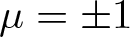 $\mu=\pm1$ need to be controlled. There we generalize the processing method described in [Reference Boutet de Monvel, Karpenko and Shepelsky5] and further using the RH method to study the high-order pole solutions of cCH equation with linear dispersion term
 $\nu u_{x}$. Then the solution of RH problem is used to construct the explicit and implicit expressions of the potential function u. Finally, we use the solution of RH problem to construct the high-order pole solutions of the cCH equation and analyse the propagation characteristics of solutions through some examples.
Acknowledgements
The authors express their sincere thanks to the anonymous reviewer for careful reading and corrections of this article, constructive comments, and suggestions for improving the quality of this article. This work was supported by the National Natural Science Foundation of China under Grant Nos. 12371255 and 11975306, Xuzhou Basic Research Program Project under Grant No. KC23048, the Six Talent Peaks Project in Jiangsu Province under Grant No. JY-059, the 333 Project in Jiangsu Province, the Fundamental Research Funds for the Central Universities under the Grant No. 2024ZDPYJQ1003, the Postgraduate Research & Practice Program of Education & Teaching Reform of CUMT under Grant No. 2023YJSJG050.