1 Introduction
Boundary-layer flows subject to an adverse pressure gradient can separate from the boundary and exhibit recirculation regions characterized by closed streamlines. The non-parallel flow regions associated with separation, in particular near the stagnation points, are likely to be responsible for the emergence of different types of instabilities. Closed streamlines may induce three-dimensional centrifugal-type instabilities as well as elliptic instability mechanisms, which has been shown for instance for backward-facing step flow (Barkley, Gomes & Henderson Reference Barkley, Gomes and Henderson2002; Beaudoin et al. Reference Beaudoin, Cadot, Aider and Wesfreid2004; Lanzerstorfer & Kuhlmann Reference Lanzerstorfer and Kuhlmann2012) or for a flow over a bump (Gallaire, Marquillie & Ehrenstein Reference Gallaire, Marquillie and Ehrenstein2007).
Two-dimensional self-sustained oscillatory instabilities with perturbation flow structures localized in the shear layer along the base flow separating streamline have been observed for instance in open cavity flows (Sipp & Lebedev Reference Sipp and Lebedev2007). Similar global two-dimensional oscillatory instabilities have also been predicted in Ehrenstein & Gallaire (Reference Ehrenstein and Gallaire2008) for a separated boundary layer induced by a bump. Model separation bubbles have been addressed for instance in Rodríguez, Gennaro & Juniper (Reference Rodríguez, Gennaro and Juniper2013), questioning the existence of a two-dimensional global oscillator behaviour.
The existence of an unstable global mode gives rise to a so-called resonator dynamics, contrary to an amplifier dynamics, which is likely to be observed in open shear flows even in the absence of individual instability modes. Indeed, the non-normality of the linear stability operator for those base flows (Schmid & Henningson Reference Schmid and Henningson2001; Schmid Reference Schmid2007) may provide a powerful instability mechanism, associated with the non-normal coupling between individually stable (or weakly unstable) modes.
The optimal control of both the resonator and the amplifier dynamics is a matter of active research (Kim & Bewley Reference Kim and Bewley2007; Cattafesta & Sheplak Reference Cattafesta and Sheplak2011; Duriez, Brunton & Noack Reference Duriez, Brunton and Noack2017). Efficient algorithms, capable of controlling flows that are both resonators and amplifiers in nature, have however still to be proposed. Recently Gautier & Aider (Reference Gautier and Aider2013, Reference Gautier and Aider2014) successfully implemented an experimental feedback control of the amplifier dynamics in a backward-facing step flow, but the control of the resonator dynamics associated with the globally unstable configuration for such a flow geometry remains an open issue. Feedback control based on a reduced-order model of the linear instability dynamics has received a lot of attention recently (Kim & Bewley Reference Kim and Bewley2007), but proved to lack robustness when considering self-sustained nonlinear dynamics (Huang & Kim Reference Huang and Kim2008; Barbagallo, Sipp & Schnmid Reference Barbagallo, Sipp and Schnmid2009; Ehrenstein, Passaggia & Gallaire Reference Ehrenstein, Passaggia and Gallaire2011). Passaggia & Ehrenstein (Reference Passaggia and Ehrenstein2013) attempted to control the nonlinear dynamics in a separated boundary-layer flow over a bump using the augmented Lagrangian approach, the control being determined iteratively by coupling the Navier–Stokes equations with the associated adjoint system. While in this approach the unstable dynamics could be attenuated, the complete control of the flow structure back to a steady state could however not be achieved. Another control strategy is to manipulate separated base flows using Lagrangian-based sensitivity analysis. For instance, Boujo & Gallaire (Reference Boujo and Gallaire2014) designed a steady actuation approach to modify quantities of interest such as the recirculation length or the geometry of the recirculation bubble’s separatrix.
The separated flow case used in the present analysis is the two-dimensional boundary-layer flow over a shallow bump, which has previously been considered in the numerical investigation by Marquillie & Ehrenstein (Reference Marquillie and Ehrenstein2003) and in the experimental study by Passaggia, Leweke & Ehrenstein (Reference Passaggia, Leweke and Ehrenstein2012). The control of this separated flow case is particularly challenging, given that its instability dynamics exhibits strong transient growth as well as multiple unstable time scales, as shown in Ehrenstein & Gallaire (Reference Ehrenstein and Gallaire2008). A simple open-loop control procedure for this flow case was designed in Boujo, Ehrenstein & Gallaire (Reference Boujo, Ehrenstein and Gallaire2013). Steady wall suction at the bump summit was found to decrease the recirculation length and proved to be capable of suppressing the unstable nature of the flow. This suction-type control hence appears as a natural starting point for a control strategy. In the present investigation, we precisely combine a sensitivity analysis and an optimal control strategy. The flow actuation is achieved by suction at the bump’s summit, aiming at controlling the flow back to its steady state for a time vanishing suction amplitude. In the present approach, the control of the slow and fast flow dynamics will first be addressed separately. Both methodologies are then combined in an optimal control strategy, which is applied to our separated flow example for increasing Reynolds numbers.
The paper is organized as follows. In § 2, the flow geometry and the numerical simulation procedure are briefly outlined. The control procedure consists of four steps which are outlined as follows.
-
(i) The sensitivity of the base flow with respect to a steady forcing is described in § 3, the key quantity for the base flow modification being the recirculation area.
-
(ii) The step response of the flow is then analysed in § 4 to determine the modal properties of the slow base flow modification dynamics.
-
(iii) An ad hoc suction control law for this slow base flow modification is determined explicitly in § 5.1 by considering a reduced-order model of the recirculation area modification.
-
(iv) This suction control law is further optimized in § 5.2 using Lagrangian-based optimal control over small time windows. The time marching is based on a receding-predictive algorithm (Bewley, Moin & Temam Reference Bewley, Moin and Temam2001) in order to suppress the fast transient dynamics.
Results are shown for different Reynolds numbers in § 6 and conclusions are given in § 7.
2 Geometry and steady state simulation procedure
2.1 Problem set-up
The fluid motion is governed by the two-dimensional incompressible Navier–Stokes system written in dimensionless form
 $$\begin{eqnarray}[\unicode[STIX]{x2202}_{t}\boldsymbol{U};\;0]=\boldsymbol{F}(\boldsymbol{U},P,Re),\quad \text{with}~\boldsymbol{F}(\boldsymbol{U},P,Re)=\left[-(\boldsymbol{U}\boldsymbol{\cdot }\unicode[STIX]{x1D735})\boldsymbol{U}-\unicode[STIX]{x1D735}P+\frac{1}{Re}\unicode[STIX]{x1D6FB}^{2}\boldsymbol{U};\;\unicode[STIX]{x1D735}\boldsymbol{\cdot }\boldsymbol{U}\right]\quad\end{eqnarray}$$
for the velocity field
 $\boldsymbol{U}(x,y,t)$
and the pressure
 $P(x,y,t)$
. The Reynolds number in (2.1) is
 $Re=\unicode[STIX]{x1D6FF}^{\ast }U_{\infty }/\unicode[STIX]{x1D708}$
, where the displacement thickness
 $\unicode[STIX]{x1D6FF}^{\ast }$
of the Blasius profile imposed at inflow
 $x=0$
is used as reference length. The free stream velocity
 $U_{\infty }$
is the reference velocity and
 $\unicode[STIX]{x1D708}$
is the dynamic viscosity. The two-dimensional flow domain is
 $0\leqslant x\leqslant L$
,
 $\unicode[STIX]{x1D702}(x)\leqslant y<y_{max}$
, with
 $\unicode[STIX]{x1D702}(x)$
the lower boundary containing a bump of height
 $h$
. The summit of the bump is localized at
 $x=25$
. According to a previous numerical analysis for this flow geometry (Marquillie & Ehrenstein Reference Marquillie and Ehrenstein2003), a domain length
 $L=250$
and upper free stream boundary
 $y_{max}=100$
are convenient to minimize finite domain effects. The free stream condition
 $(U,V)=(1,0)$
has been imposed whereas no-slip conditions are used at the wall
 $y=\unicode[STIX]{x1D702}(x)$
. The stress-free boundary condition
 $$\begin{eqnarray}\frac{1}{Re}(\unicode[STIX]{x1D735}\boldsymbol{U})\boldsymbol{\cdot }\boldsymbol{n}|_{x=L}=P\boldsymbol{n}|_{x=L}\end{eqnarray}$$
(
 $\boldsymbol{n}$
being the unit normal vector at the flow domain’s boundary) has been implemented at the outflow
 $x=L$
and it proved to be appropriate for both the simulations and the subsequent optimization procedures. The streamwise direction
 $x$
is discretized using fourth-order finite differences, whereas in the wall-normal direction
 $y$
Chebyshev collocation is considered and the pressure is solved using the influence matrix technique. Details about the numerical discretization procedure can be found in Marquillie & Ehrenstein (Reference Marquillie and Ehrenstein2002) and Passaggia & Ehrenstein (Reference Passaggia and Ehrenstein2013).
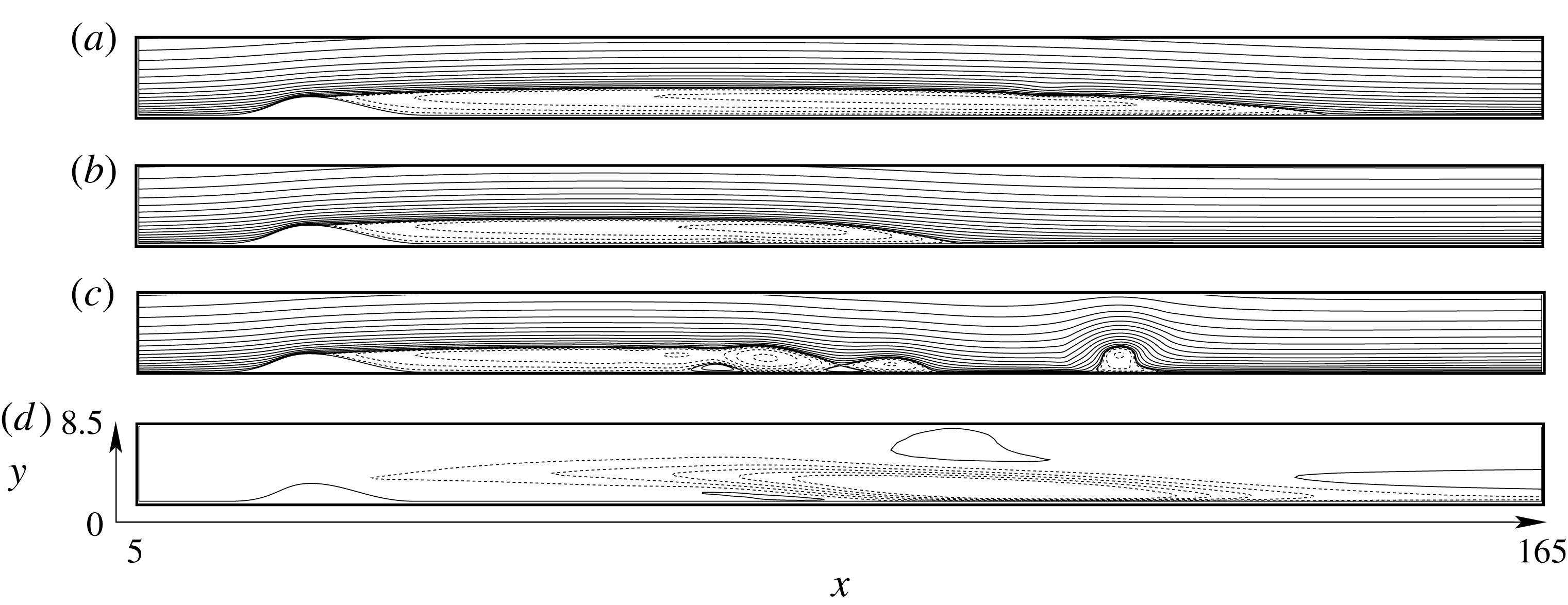
Streamlines of the base flow
 $\boldsymbol{Q}_{0}$
(a), of the mean flow
 $\bar{\boldsymbol{Q}}$
(b) and of a snapshot of the unstable flow field (c), at
 $Re=650$
and a bump height
 $h=2$
(the values of the iso-contours are chosen arbitrarily to represent the flow dynamics). Base flow modification
 $\unicode[STIX]{x1D6FF}\boldsymbol{Q}=\boldsymbol{Q}_{0}-\bar{\boldsymbol{Q}}$
(d), shown by iso-contours of streamwise velocity
 $u$
in the range
 $[-0.35,-0.28,-0.23,\ldots ,0.13]$
, the dashed/continuous lines being the negative/positive values respectively.

2.2 Selective frequency damping method
Steady state solutions of the Navier–Stokes system and its adjoint are computed using the selective frequency damping technique (SFD) proposed in Åkervik et al. (Reference Åkervik, Brandt, Henningson, Hœpffner, Marxen and Schlatter2006). Writing formally the Navier–Stokes equations
 $\unicode[STIX]{x2202}_{t}\boldsymbol{Q}=\boldsymbol{F}(\boldsymbol{Q},Re)$
, the method consists in solving the coupled system
 $$\begin{eqnarray}\left.\begin{array}{@{}c@{}}\unicode[STIX]{x2202}_{t}\boldsymbol{Q}=\boldsymbol{F}(\boldsymbol{Q},Re)-\unicode[STIX]{x1D701}(\boldsymbol{Q}-\boldsymbol{R}),\\ \unicode[STIX]{x2202}_{t}\boldsymbol{R}=\displaystyle \frac{1}{\unicode[STIX]{x1D6EC}}(\boldsymbol{Q}-\boldsymbol{R}).\end{array}\right\}\end{eqnarray}$$
The coupled system (2.3) is integrated in time by computing a sliding time average
 $\boldsymbol{R}(t)$
of the flow dynamics
 $\boldsymbol{Q}(t)$
and subtracting their difference in the Navier–Stokes equations. The parameter
 $\unicode[STIX]{x1D6EC}$
is the time window over which the sliding average
 $\boldsymbol{R}$
is computed. The damping factor
 $\unicode[STIX]{x1D701}$
is akin to a decay rate and has to be sufficiently large to allow for filtering the instabilities from the solution
 $\boldsymbol{Q}$
as the system (2.3) is integrated in time. Once the above algorithm has converged, that is
 $\unicode[STIX]{x2202}_{t}\boldsymbol{Q}=\unicode[STIX]{x2202}_{t}\boldsymbol{R}=0$
, the solution
 $\boldsymbol{R}=\boldsymbol{Q}$
is the steady state solution of (2.1). Here we use the procedure of Cunha, Passaggia & Lazareff (Reference Cunha, Passaggia and Lazareff2015) to compute optimal parameters for the SFD. For instance at
 $Re=650$
, the best stabilization strategy was found for
 $(\unicode[STIX]{x1D701},\unicode[STIX]{x1D6EC})=(0.0292,14.99)$
. The resulting steady state, which in the following will be written
 $\boldsymbol{Q}_{0}$
, is shown in figure 1(a). As can be seen, the flow separates at the bump summit and the steady state is characterized by an elongated recirculation bubble which reattaches at
 $x\approx 125$
for the specific supercritical Reynolds number
 $Re=650$
and bump height
 $h=2$
chosen.
Note that the critical Reynolds number for the onset of the two-dimensional global unstable dynamics for this bump flow geometry has been found to be
 $Re_{c}\approx 590$
in the numerical investigation by Marquillie & Ehrenstein (Reference Marquillie and Ehrenstein2003). This critical Reynolds number range has more recently been confirmed experimentally in Passaggia et al. (Reference Passaggia, Leweke and Ehrenstein2012).
2.3 Steady and mean state
The two-dimensional self-sustained instabilities associated with the present flow geometry have already been investigated (Marquillie & Ehrenstein Reference Marquillie and Ehrenstein2002, Reference Marquillie and Ehrenstein2003; Ehrenstein & Gallaire Reference Ehrenstein and Gallaire2008; Passaggia et al.
Reference Passaggia, Leweke and Ehrenstein2012). In particular, it has been shown that in the unstable regime the time-averaged mean flow exhibits a shorter recirculation bubble, the length of which decreasing with increasing Reynolds number. A numerical simulation of the developed unstable flow at
 $Re=650$
(figure 1(c) showing a snapshot sample of the unsteady flow field) was performed to compute the mean state by time averaging
 $$\begin{eqnarray}\bar{\boldsymbol{Q}}=\frac{1}{\unicode[STIX]{x0394}t}\int _{t}^{t+\unicode[STIX]{x0394}t}\boldsymbol{Q}(\boldsymbol{x},t)\,\text{d}t,\end{eqnarray}$$
with
 $\unicode[STIX]{x0394}t=4000$
in the above integral. The corresponding mean flow is shown in figure 1(b). The difference
 $$\begin{eqnarray}\unicode[STIX]{x1D6FF}\boldsymbol{Q}=\boldsymbol{Q}_{0}-\bar{\boldsymbol{Q}}\end{eqnarray}$$
between the steady state and the mean flow state plays an important role in the dynamics and
 $\unicode[STIX]{x1D6FF}\boldsymbol{Q}$
, shown in figure 1(d) for the flow case at
 $Re=650$
considered, will be seen to be a key quantity for the control of this flow configuration.
The effects of a small modification of the steady state on self-excited flows characterized by a strong dominant frequency was addressed for instance by Sipp & Lebedev (Reference Sipp and Lebedev2007) in the case of a separated boundary-layer flow over a square cavity and more recently by Turton, Tuckerman & Barkley (Reference Turton, Tuckerman and Barkley2015) in the case of thermosolutal convection. The latter showed that the linearized operator around the mean flow indeed exhibits a purely imaginary eigenvalue that predicts the nonlinear frequency of the instability. The linearized mean flow dynamics has been considered by Mantič-Lugo, Arratia & Gallaire (Reference Mantič-Lugo, Arratia and Gallaire2014, Reference Mantič-Lugo, Arratia and Gallaire2015) to build a self-consistent model of the cylinder flow that predicts both the frequency of the vortex shedding and the amplitude of the nonlinear limit cycle for Reynolds numbers up to
 $110$
. Flinois & Colonius (Reference Flinois and Colonius2015) showed that fully developed nonlinear flow dynamics of the cylinder flow could be controlled using a direct–adjoint approach, by optimizing the control law of blowing and suction actuators located at the walls of the cylinder. But the conclusions of these studies cannot be extended to the more general case where a flow presents a broadband spectrum of unstable frequencies. The attempts in Passaggia & Ehrenstein (Reference Passaggia and Ehrenstein2013) to control the unstable flow dynamics for the present separated boundary-layer flow led to the conclusion that while the instabilities of the fully developed regime could be attenuated using an direct–adjoint optimization of the nonlinear dynamics, the flow could however not be controlled back to its steady state. The complex dynamics involving unstable global modes and transient growth led to increasingly large time optimization windows with increasing Reynolds numbers, making the optimization problem hardly tractable in the strongly unstable regime.
In the following, we revisit the control problem for this challenging separated bump flow problem. Our approach will consist in a suction-like actuation to control the steady state modification
 $\unicode[STIX]{x1D6FF}\boldsymbol{Q}$
in combination with a direct–adjoint iterative optimization procedure to minimize transient growth phenomena and global instabilities. We first consider the sensitivity analysis of the bump flow for a steady suction-type forcing following the Lagrangian optimization approach of Boujo & Gallaire (Reference Boujo and Gallaire2014), which was capable of damping and even suppress the self-excited instabilities (Boujo, Gallaire & Ehrenstein Reference Boujo, Gallaire and Ehrenstein2014). We therefore seek to compute first the most sensitive region of the flow to a wall suction actuator with the aim of maximizing the controllability while minimizing the size of the actuator.
3 Sensitivity analysis
The base flow modification
 $\unicode[STIX]{x1D6FF}\boldsymbol{Q}$
shown in figure 1(d) drastically reduces the length but also the structure of the recirculation region (e.g. the angles of the separatrix near the separation/reattachment points or the amount of backflow). Therefore we consider here the sensitivity of the recirculation area
 $A_{rec}$
which is an integral quantity defined as
 $$\begin{eqnarray}A_{rec}(t)=\int _{x_{s}(t)}^{x_{r}(t)}\int _{\unicode[STIX]{x1D702}(x)}^{y_{sep}(x,t)}\,\text{d}x\,\text{d}y,\end{eqnarray}$$
where
 $x_{s,r}$
are the locations of the separation/reattachment point at the wall and
 $y_{sep}(x,t)$
is the height of the separatrix, defined as the streamline which connects the stagnation points. Note that in the time-dependent setting, instabilities can be strong enough to create multiple stagnation points along the wall, within the recirculation region (Haller Reference Haller2004; Weldon et al.
Reference Weldon, Peacock, Jacobs, Helu and Haller2008). In the present analysis, the base flow modification will however be seen to be a slowly varying process. Therefore, in the absence of fluctuations, a separation point
 $x_{s}(t)$
as well as a stagnation location
 $x_{r}(t)$
on the wall beyond which the flow remains attached can be identified for the computation of the integral (3.1). In the remaining of this subsection the dependence on time for the sensitivity analysis is dropped. This is justified because, as already mentioned, the actuation
 $\unicode[STIX]{x1D6F7}(t)$
is assumed to be slow compared with the time scale of instabilities. This assumption will be supported by the dynamic modes decomposition (DMD) analysis in § 4.1. The time dependence will be reintroduced later to minimize the recirculation area modification
 $\unicode[STIX]{x1D6FF}A_{rec}$
which is associated with the base flow modification
 $\unicode[STIX]{x1D6FF}\boldsymbol{Q}$
. The sensitivity of a steady state to a modification of the recirculation area reduces to a field defined through the first-order modification
 $\unicode[STIX]{x1D6FF}A_{rec}$
, induced by a small amplitude steady blowing–suction control
 $\unicode[STIX]{x1D6FF}\unicode[STIX]{x1D6F7}$
at the wall
 $\unicode[STIX]{x1D6E4}_{c}$
and is given by
 $$\begin{eqnarray}\unicode[STIX]{x1D6FF}A_{rec}=(\unicode[STIX]{x1D735}_{\unicode[STIX]{x1D6F7}}A_{rec}|\unicode[STIX]{x1D6FF}\unicode[STIX]{x1D6F7}).\end{eqnarray}$$
Here
 $(\cdot |\cdot )$
is the inner product between
 $\unicode[STIX]{x1D735}_{\unicode[STIX]{x1D6F7}}A_{rec}$
(i.e. the gradient of the recirculation area with respect to the suction forcing) and the small modification of suction amplitude
 $\unicode[STIX]{x1D6FF}\unicode[STIX]{x1D6F7}$
. Note that in the present study there is only one actuator. Hence
 $\unicode[STIX]{x1D6F7}$
is simply a scalar quantity and the above inner product is a simple product between scalars. The actuator is defined by the shape function
 $\boldsymbol{B}$
, which corresponds to the unit vector. This shape function is orthogonal to
 $\unicode[STIX]{x1D702}(x)$
along
 $\unicode[STIX]{x1D6E4}_{c}$
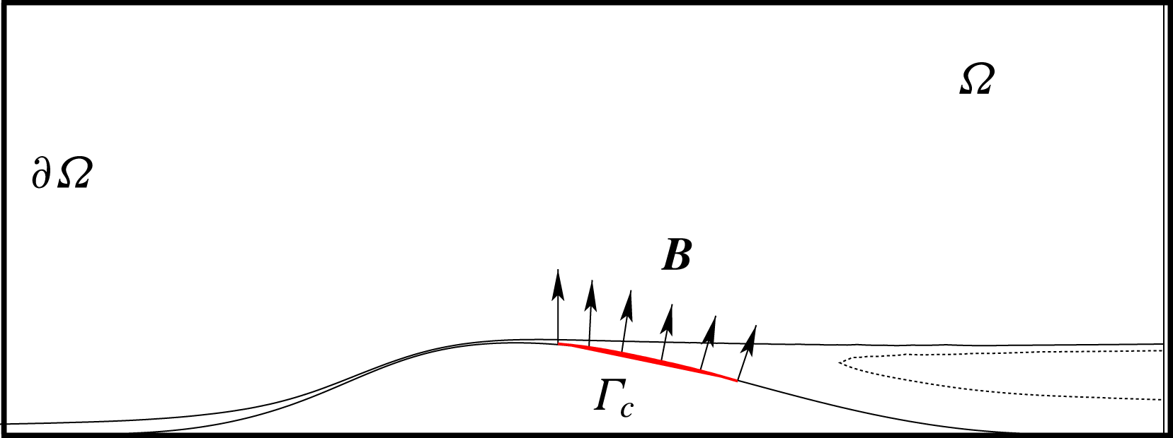
on the portion of the boundary where the control is applied (cf. figure 2).
Sketch of the domain and of the control set-up. The actuator
 $\boldsymbol{B}$
is located on the wall along the surface
 $\unicode[STIX]{x1D6E4}_{c}$
, located on the boundary
 $\unicode[STIX]{x1D702}(x)=[25,30]$
.

The Lagrange multipliers
 $\boldsymbol{Q}^{+}$
are introduced and the Lagrangian
 $$\begin{eqnarray}{\mathcal{L}}(\boldsymbol{Q},\boldsymbol{Q}^{+})=A_{rec}-\langle \boldsymbol{F}(\boldsymbol{Q},Re),\boldsymbol{Q}^{+}\rangle -\int _{\unicode[STIX]{x1D6E4}_{c}}\boldsymbol{g}(\boldsymbol{U},\unicode[STIX]{x1D6F7})\boldsymbol{\cdot }\boldsymbol{B}\unicode[STIX]{x1D6F7}^{+}\,\text{d}\boldsymbol{s}\end{eqnarray}$$
is to be rendered stationary. The scalar product
 $\langle \cdot \,,\cdot \rangle$
is defined by the integral
 $\int _{\unicode[STIX]{x1D6FA}}\;\cdot \;\text{d}\boldsymbol{x}$
where
 $\unicode[STIX]{x1D6FA}$
is the flow domain. The boundary condition for the velocity field at
 $\unicode[STIX]{x1D6E4}_{c}$
associated with the control
 $\unicode[STIX]{x1D6F7}$
 $$\begin{eqnarray}\boldsymbol{g}(\boldsymbol{U},\unicode[STIX]{x1D6F7})=\boldsymbol{U}|_{\unicode[STIX]{x1D6E4}_{c}}-\boldsymbol{B}\unicode[STIX]{x1D6F7}=0\end{eqnarray}$$
is added to the Lagrangian with
 $\unicode[STIX]{x1D6F7}^{+}$
the Lagrange multiplier associated with the control
 $\unicode[STIX]{x1D6F7}$
. The adjoint Navier–Stokes system is derived from (3.3) by taking the Fréchet derivative defined such that
 $$\begin{eqnarray}{\mathcal{L}}_{\boldsymbol{Q}}(\boldsymbol{Q},\boldsymbol{Q}^{+})\boldsymbol{\cdot }\hat{\boldsymbol{Q}}=\lim _{\unicode[STIX]{x1D716}\rightarrow 0}\frac{1}{\unicode[STIX]{x1D716}}[{\mathcal{L}}(\boldsymbol{Q}+\unicode[STIX]{x1D716}\hat{\boldsymbol{Q}},\boldsymbol{Q}^{+})-{\mathcal{L}}(\boldsymbol{Q},\boldsymbol{Q}^{+})]\end{eqnarray}$$
with respect to
 $\boldsymbol{Q}$
(see Joslin et al. (Reference Joslin, Gunzburger, Nicolaides, Erlebacher and Hussaini1995)) and is given by
 $$\begin{eqnarray}\boldsymbol{F}^{+}(\boldsymbol{U},\boldsymbol{Q}^{+},Re)=\biggl[-(\boldsymbol{U}\boldsymbol{\cdot }\unicode[STIX]{x1D735})\boldsymbol{U}^{+}+(\unicode[STIX]{x1D735}\boldsymbol{U})^{\text{T}}\boldsymbol{U}^{+}+\unicode[STIX]{x1D735}P^{+}-\frac{1}{Re}\unicode[STIX]{x1D6FB}^{2}\boldsymbol{U}^{+};-\unicode[STIX]{x1D735}\boldsymbol{\cdot }\boldsymbol{U}^{+}\biggr].\end{eqnarray}$$
The boundary terms are given by
 $$\begin{eqnarray}\int _{\unicode[STIX]{x2202}\unicode[STIX]{x1D6FA}}\bigg[\frac{1}{Re}\boldsymbol{U}^{+}(\unicode[STIX]{x1D735}\hat{\boldsymbol{U}}\boldsymbol{\cdot }\boldsymbol{n})-\frac{1}{Re}(\unicode[STIX]{x1D735}\boldsymbol{U}^{+}\boldsymbol{\cdot }\boldsymbol{n})\hat{\boldsymbol{U}}-(\boldsymbol{U}\boldsymbol{\cdot }\boldsymbol{n})\boldsymbol{U}^{+}\boldsymbol{\cdot }\hat{\boldsymbol{U}}+(P^{+}\boldsymbol{\cdot }\boldsymbol{n})\hat{\boldsymbol{U}}-\boldsymbol{U}^{+}(\hat{P}\boldsymbol{\cdot }\boldsymbol{n})\bigg]\,\text{d}\boldsymbol{s},\end{eqnarray}$$
with
 $\boldsymbol{n}$
the unit vector normal to the boundary
 $\unicode[STIX]{x2202}\unicode[STIX]{x1D6FA}$
. The boundary conditions for the velocity field
 $\boldsymbol{U}$
are
 $$\begin{eqnarray}\frac{1}{Re}(\unicode[STIX]{x1D735}\boldsymbol{U})\boldsymbol{\cdot }\boldsymbol{n}|_{x=L}=P\boldsymbol{n}|_{x=L},\quad \boldsymbol{U}|_{x=0}=(U_{Blas}(y),0),\quad \boldsymbol{U}|_{y=\unicode[STIX]{x1D702}}=0,\quad \boldsymbol{U}|_{y=H}=1,\end{eqnarray}$$
where
 $U_{Blas}$
is the Blasius velocity profile imposed at the inlet. The same conditions hold for all possible variations in
 $\hat{\boldsymbol{U}}$
and
 $\hat{P}$
in the Fréchet derivatives. The boundary integral in (3.7) therefore vanishes when the boundary conditions for the adjoint system
 $$\begin{eqnarray}\frac{1}{Re}(\unicode[STIX]{x1D735}\boldsymbol{U}^{+})\boldsymbol{n}+(\boldsymbol{U}\boldsymbol{\cdot }\boldsymbol{n})\boldsymbol{U}^{+}|_{x=0,L}=P^{+}\boldsymbol{n}|_{x=0,L},\quad \boldsymbol{U}^{+}|_{y=\unicode[STIX]{x1D702},H}=0\end{eqnarray}$$
are considered. The adjoint system (3.6) is subject to a source term related to the
 $A_{rec}$
term in (3.3). The flow rate through any vertical cross-section of the recirculation region is zero and using this property Boujo & Gallaire (Reference Boujo and Gallaire2014) showed that
 $$\begin{eqnarray}\langle \unicode[STIX]{x1D735}_{\boldsymbol{Q}}A_{rec},\hat{\boldsymbol{Q}}\rangle =\int _{x_{s}}^{x_{r}}\frac{-1}{U(x,y_{sep}(x))}\left(\int _{y_{w(x)}}^{y_{sep(x)}}\hat{U} \,\text{d}y\right)\,\text{d}x.\end{eqnarray}$$
According to this formula, the adjoint system to solve is
 $$\begin{eqnarray}\boldsymbol{F}^{+}(\boldsymbol{U},\boldsymbol{Q}^{+},Re)=[h(U);0;0],\quad \text{with}~h(U)=\int _{x_{s}}^{x_{r}}\frac{-1}{U(x,y_{sep}(x))}\left(\int _{y_{w(x)}}^{y_{sep(x)}}\,\text{d}y\right)\,\text{d}x.\end{eqnarray}$$
Similar to the procedure used for the solution of (2.1), this adjoint system subject to the conditions (3.9) is solved using the influence matrix technique outlined in Passaggia & Ehrenstein (Reference Passaggia and Ehrenstein2013). The steady state adjoint solution
 $\boldsymbol{Q}^{+}$
is obtained through time marching of (3.6), coupled to the selective frequency damping method (cf. §2). The adjoint solution for
 $\boldsymbol{U}^{+}$
is shown in figure 3 at
 $Re=650$
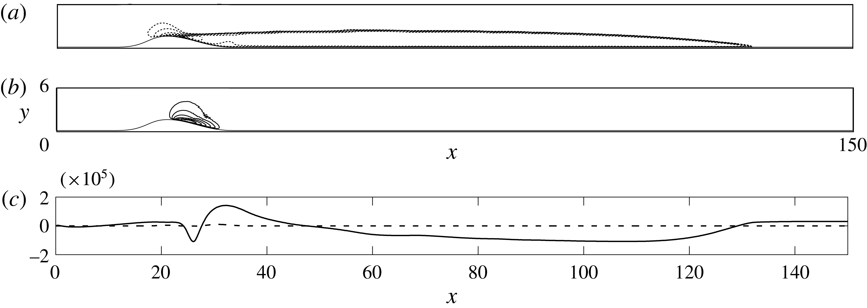
, where the most sensitive region to blowing or suction is identified in the vicinity of the separation point.
Contours of the adjoint solutions
 $U^{+}$
(a) and
 $V^{+}$
(b) for the sensitivity of the recirculation area
 $A_{rec}$
at
 $Re=650$
. The continuous/dotted lines represent positive/negative contours respectively. (c) Values of the gradient
 $-Re^{-1}\unicode[STIX]{x1D735}\boldsymbol{U}^{+}\boldsymbol{\cdot }\boldsymbol{n}+P^{+}\boldsymbol{n}$
evaluated at
 $\unicode[STIX]{x1D702}_{x}$
for the first component (- - - -) and the second component (——).

There are remaining terms in the boundary integral (3.7). According to the Fréchet derivative of the third term in the Lagrangian (3.3) and taking into account (3.4), these terms cancel when
 $$\begin{eqnarray}\boldsymbol{B}\unicode[STIX]{x1D6F7}^{+}=-\frac{1}{Re}\unicode[STIX]{x1D735}\boldsymbol{U}^{+}\boldsymbol{\cdot }\boldsymbol{n}+P^{+}\,\boldsymbol{n}\end{eqnarray}$$
on
 $\unicode[STIX]{x1D6E4}_{c}$
. Taking the derivative of the Lagrangian with respect to
 $\unicode[STIX]{x1D6F7}$
and taking into account (3.12) one recovers the gradient
 $$\begin{eqnarray}\unicode[STIX]{x1D735}_{\unicode[STIX]{x1D6F7}}A_{rec}=\int _{\unicode[STIX]{x1D6E4}_{c}}\left(-\frac{1}{Re}\unicode[STIX]{x1D735}\boldsymbol{U}^{+}\boldsymbol{\cdot }\boldsymbol{n}+P^{+}\boldsymbol{n}\right)\boldsymbol{\cdot }\boldsymbol{B}\,\text{d}\boldsymbol{s}.\end{eqnarray}$$
This expression is used in (3.2), providing the modification of the recirculation bubble area
 $\unicode[STIX]{x1D6FF}A_{rec}$
as a function of the suction amplitude
 $\unicode[STIX]{x1D6FF}\unicode[STIX]{x1D6F7}$
.
In the following section, we address the design of a control strategy for the base flow modification. The underlying idea is that a (steady) suction induces a base flow modification and in particular a shortening of the recirculation bubble, which is expected to be qualitatively similar to the action of the unstable dynamics on the time-averaged mean flow. The dynamics of the base flow modification due to suction that is the transition back to the original steady state (obtained by solving the SFD system (cf. § 2.2)) will be characterized in terms of modes applying a dynamic modes decomposition (DMD) which is briefly outlined in appendix A.
4 Step response to a base flow modification
We use the hypothesis, that the transition from the modified base flow back to the steady state is a modal-type dynamics
 $\unicode[STIX]{x1D6FF}\boldsymbol{Q}\text{e}^{\unicode[STIX]{x1D70E}t}$
, with a spatial distribution
 $\unicode[STIX]{x1D6FF}\boldsymbol{Q}$
(the base flow modification) and a decay rate
 $\unicode[STIX]{x1D70E}$
, similar to the shift mode described by Noack et al. (Reference Noack, Konstantin, Morzyński, Tadmor and Thiele2003) in the case of the cylinder flow. To determine the characteristics of this mode, we consider the step response of the Navier–Stokes equations corresponding to the dynamics of a modified base flow with a shorter recirculation bubble set free to evolve back to the steady state.
However, self-excited instabilities prevent the flow returning to the steady state and the step response is therefore applied to the SFD system (2.3) designed to stabilize the Navier–Stokes dynamics. We hereafter briefly outline how the dynamics for the Navier–Stokes system can be inferred from the knowledge about the (stabilized) dynamics of the SFD system. As shown by Åkervik et al. (Reference Åkervik, Brandt, Henningson, Hœpffner, Marxen and Schlatter2006) and Jordi, Cotter & Sherwin (Reference Jordi, Cotter and Sherwin2014), the linear perturbation dynamics evaluated close to a steady state of the Navier–Stokes system (2.1) is related to the linear perturbation dynamics of (2.3) by a transfer function. Indeed, the action of the SFD coupled to the Navier–Stokes equations in the system (2.3) can be described by a first-order bandpass time filter of the form (Åkervik et al. Reference Åkervik, Brandt, Henningson, Hœpffner, Marxen and Schlatter2006)
 $$\begin{eqnarray}\boldsymbol{R}(\boldsymbol{x},T)=\int _{-\infty }^{T}\frac{1}{\unicode[STIX]{x1D6EC}}\exp \left(\frac{\unicode[STIX]{x1D70F}-T}{\unicode[STIX]{x1D6EC}}\right)\boldsymbol{Q}(\boldsymbol{x},\unicode[STIX]{x1D70F})\,\text{d}\unicode[STIX]{x1D70F}.\end{eqnarray}$$
Performing a Fourier–Laplace transform of the time filter gives
 $$\begin{eqnarray}\int _{-\infty }^{0}\frac{1}{\unicode[STIX]{x1D6EC}}\exp \left(\frac{\unicode[STIX]{x1D70F}}{\unicode[STIX]{x1D6EC}}\right)\exp (-\text{i}\unicode[STIX]{x1D714}\unicode[STIX]{x1D70F})\,\text{d}\unicode[STIX]{x1D70F}=\frac{1}{1-\text{i}\unicode[STIX]{x1D714}\unicode[STIX]{x1D6EC}},\end{eqnarray}$$
where the real part of
 $\unicode[STIX]{x1D714}$
is the circular frequency. Thus we get the equality for the Laplace transforms
 $$\begin{eqnarray}L(\boldsymbol{R})=\frac{1}{1-\text{i}\unicode[STIX]{x1D714}\unicode[STIX]{x1D6EC}}L(\boldsymbol{Q}).\end{eqnarray}$$
Using this property, the transfer function associated with the SFD system (2.3) provides a linear transformation between the stabilized eigenvalues
 $\unicode[STIX]{x1D70E}_{SFD}$
back to their Navier–Stokes counterparts
 $\unicode[STIX]{x1D70E}$
. Here
 $-\text{i}\unicode[STIX]{x1D714}$
is to be substituted with the stabilized eigenvalue
 $\unicode[STIX]{x1D70E}_{SFD}$
. Introducing (4.3) in (2.3), the dynamics of the Navier–Stokes base flow modification without the low-pass filter is characterized by the decay rate
 $\unicode[STIX]{x1D70E}$
through the relation
 $$\begin{eqnarray}\unicode[STIX]{x1D70E}=\unicode[STIX]{x1D70E}_{SFD}+\unicode[STIX]{x1D701}\left(1-\frac{1}{1+\unicode[STIX]{x1D70E}_{SFD}\;\unicode[STIX]{x1D6EC}}\right).\end{eqnarray}$$
In the following, a base flow subject to a control is computed as solution of the SFD system (2.3). Once the suction suppressed, the evolution of the flow state with control back to the original steady state is characterized by a dynamic mode decomposition (Schmid Reference Schmid2010), integrating in time system (2.3). In this procedure, the base flow modification decay rate
 $\unicode[STIX]{x1D70E}_{SFD}$
is recovered and the associated rate for the Navier–Stokes system is computed using (4.4).
The control is performed by adding a blowing and suction actuator located at the summit of the bump (cf. figure 2).
 $\unicode[STIX]{x1D6E4}_{c}$
denotes the portion of the domain over which the control is applied and was chosen along the boundary
 $\unicode[STIX]{x1D702}=[25,30]$
, which proved to be the most sensitive region to a forcing. The vector
 $\boldsymbol{B}$
is the blowing profile given by the normal
 $\boldsymbol{n}$
along
 $\unicode[STIX]{x1D6E4}_{c}$
(Boujo et al.
Reference Boujo, Ehrenstein and Gallaire2013; Passaggia & Ehrenstein Reference Passaggia and Ehrenstein2013). The evolution of the state with control is obtained by first integrating the system (2.3) back to the original steady state. Then the suction is suppressed and the resulting dynamics is characterized using a dynamic mode decomposition.
4.1 Dynamic mode decomposition of the stabilized step response
Evaluating the impulse or step response of a linear system can be efficiently performed using either balanced truncations or Krylov-type methods (Antoulas Reference Antoulas2005) (the impulse response of a linear system is the time derivative of the step response, which in the forthcoming dynamic mode decomposition does not affect the frequency content of the response. The DMD analysis of the step response is thus expected to be very close to the impulse response, at least for a small enough step amplitude). In the case of nonlinear systems, the analogue to Krylov-type methods is known as dynamic mode decomposition. The DMD method consists in computing a linear approximation of a nonlinear system, solely based on snapshots of the flow (Rowley et al.
Reference Rowley, Mezić, Bagheri, Schlatter and Henningson2009; Schmid Reference Schmid2010). The initial condition of the step response is a steady state subject to a small amplitude steady suction actuation at the wall chosen as
 $\unicode[STIX]{x1D6F7}_{0}=-10^{-4}$
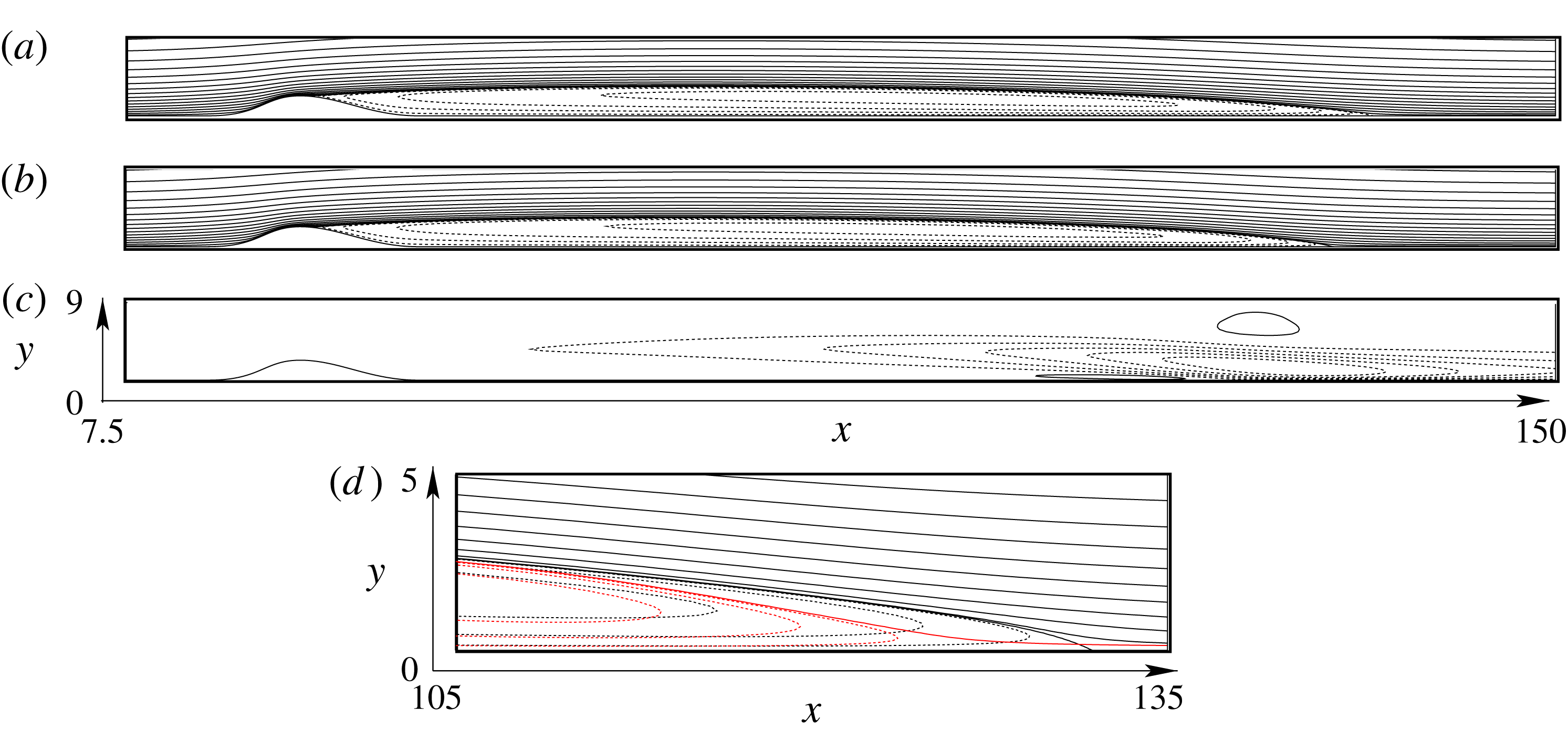
. This forcing on the stabilized dynamics produces a modified steady state with a slightly shorter recirculation bubble (see figure 4
a–d) compared with the base flow. Note that in Boujo et al. (Reference Boujo, Ehrenstein and Gallaire2013) it has been shown that such steady suction forcing with sufficient amplitude stabilizes the self-sustained instabilities.
The stabilized step response is initialized using the suction steady state shown in figure 4(b). Once this actuation is suppressed (i.e.
 $\unicode[STIX]{x1D6F7}_{0}=0$
) at
 $t=0$
, the stabilized system (2.3) is marched in time where the shorter recirculation region evolves back to its steady state shown in figure 4(a). This flow evolution is analysed using a dynamic mode decomposition (see appendix A for a description of the algorithm), which will provide the temporal mode associated with the base flow modification.
Streamlines of the base flow without (a) and with suction (b) for an amplitude
 $\unicode[STIX]{x1D6F7}_{0}=-10^{-4}$
imposed by the actuator
 $\unicode[STIX]{x1D6E4}_{c}$
at
 $Re=650$
and a bump height
 $h=2$
. Iso-contours of the streamwise velocity
 $u$
component of the base flow modification (c). The continuous lines denote the positive contours of the associated quantity while the dashed line shows the negative contours. Close up of the streamlines (d) of the steady state (black) and the suction steady state (red) near the reattachment point, the
 $y$
axis being stretched compared to the
 $x$
axis.

(a) DMD spectrum
 $(\unicode[STIX]{x1D70E}_{r},\unicode[STIX]{x1D70E}_{i})$
computed by time-marching of the SFD system (empty symbols) and the corresponding Navier–Stokes eigenvalues using the transformation (4.4) (filled symbols); steady state eigenvalue (red square ▫), eigenvalue associated with the base flow modification (○,


 $\unicode[STIX]{x1D70E}_{r}=0$
) and the corresponding transformed curve using (4.4) is depicted in grey. (b) Streamlines associated with the steady state (red square ▫) (top), iso-contours of the streamwise velocity of the least stable purely real-values mode associated with the base flow modification (middle) and iso-contours of the streamwise velocity of the most amplified mode
 $\hat{u}$
(


The DMD analysis has been performed at
 $Re=650$
and the result is shown in figure 5. The transformation (4.4) was applied to the eigenvalues
 $\unicode[STIX]{x1D70E}_{SFD}$
of the DMD spectrum obtained by time stepping of the SFD system, providing the corresponding DMD eigenvalues
 $\unicode[STIX]{x1D70E}$
for the Navier–Stokes dynamics. The least stable real mode is shown in figure 5(a) by mean of a grey circle (


 $\unicode[STIX]{x1D701}$
and
 $\unicode[STIX]{x1D6EC}$
are chosen appropriately. They also showed, that the real eigenvalues
 $\unicode[STIX]{x1D70E}$
associated with the base flow modification always increase under the action of the SFD, independently of the choice of the couple (
 $\unicode[STIX]{x1D701},\unicode[STIX]{x1D6EC}$
). This means that the stabilized decay rate
 $\unicode[STIX]{x1D70E}_{SFD}$
is always shifted towards the origin when using the SFD method, as shown by the arrow in the close up view in figure 5(a). The steady state is characterized by an eigenvalue equal to zero (i.e. the red square (▫)) in figure 5(a) and is shown in figure 5(b). The real eigenvalue (see the grey circle in the close up view near the origin in figure 5
a) is precisely associated with the base flow modification shown in figure 5(b), which is seen to be similar to the steady state modification
 $\unicode[STIX]{x1D6FF}\boldsymbol{Q}$
shown in figure 1(d). Therefore, one may assume that the base flow modification produced by the suction actuator and the base flow modification induced by the self-excited instabilities are indeed close. The most unstable oscillatory mode is also depicted in figure 5(b) and displays a very similar spatial structure as the most unstable global mode found by Ehrenstein & Gallaire (Reference Ehrenstein and Gallaire2008).
Separating the base flow dynamics from the oscillatory perturbations, we make the assumption of the following decomposition for the unsteady flow field
 $$\begin{eqnarray}\boldsymbol{Q}(\boldsymbol{x},t)=\boldsymbol{Q}_{0}(\boldsymbol{x})+\unicode[STIX]{x1D6FF}\boldsymbol{Q}(\boldsymbol{x},\boldsymbol{t})+\tilde{\boldsymbol{q}}(\boldsymbol{x},t),\end{eqnarray}$$
where
 $\tilde{\boldsymbol{q}}$
is the remaining perturbation. Note that by construction,
 $\tilde{\boldsymbol{q}}$
satisfies
 $$\begin{eqnarray}\lim _{\unicode[STIX]{x0394}t\rightarrow \infty }\frac{1}{\unicode[STIX]{x0394}t}\int _{t}^{t+\unicode[STIX]{x0394}t}\tilde{\boldsymbol{q}}(\boldsymbol{x},t)\,\text{d}t=0.\end{eqnarray}$$
In the case of the linear perturbation dynamics
 $\unicode[STIX]{x1D6FF}\boldsymbol{Q}=0$
and the perturbation is entirely contained in
 $\tilde{\boldsymbol{q}}$
. Up to now, we have focused on the evolution of the base flow and its modification, assuming that the fluctuations
 $\tilde{\boldsymbol{q}}$
are stabilized (i.e. for values of
 $Re$
below criticality or suppressed by some control), in which case the temporal evolution is written
 $$\begin{eqnarray}\boldsymbol{Q}(\boldsymbol{x},t)=\boldsymbol{Q}_{0}(\boldsymbol{x})+\unicode[STIX]{x1D6FF}\boldsymbol{Q}(\boldsymbol{x})\text{e}^{\unicode[STIX]{x1D70E}t}.\end{eqnarray}$$
It is recalled that the computed decay rate
 $\unicode[STIX]{x1D70E}$
associated with the base flow modification
 $\unicode[STIX]{x1D6FF}\boldsymbol{Q}$
is real and negative in the present study. In the next section, a methodology is developed to control the perturbation of the steady state by considering separately the control of the base flow modification
 $\unicode[STIX]{x1D6FF}\boldsymbol{Q}$
and the fluctuations induced by the instabilities
 $\tilde{\boldsymbol{q}}$
. This is motivated by the difference of time scales shown by the DMD eigenvalues in figure 5(a) between the slow base flow modification and the fast instability modes and we assume that
 $$\begin{eqnarray}\unicode[STIX]{x2202}_{t}\unicode[STIX]{x1D6FF}\boldsymbol{Q}\ll \unicode[STIX]{x2202}_{t}\tilde{\boldsymbol{q}}.\end{eqnarray}$$
Using the same actuator, two control strategies are sought separately: the control of the base flow modification will be optimized using a linear quadratic (LQ) type regulator, while the fluctuations will be controlled using an augmented Lagrangian approach of the nonlinear dynamics. It is important to note that it is not necessary to compute
 $\unicode[STIX]{x1D6FF}\boldsymbol{Q}$
explicitly. As it will be shown later, time derivatives of the flow can indeed be used to filter
 $\unicode[STIX]{x1D6FF}\boldsymbol{Q}$
from the fluctuation
 $\tilde{\boldsymbol{q}}$
.
Concerning the slow base flow dynamics, we show in the next section that an analytical expression for the control of the base flow modification can be computed. This step is necessary in order to take into account the slow dynamics when computing the control law. It has again to be emphasized that the base flow modification is precisely the pitfall of the Lagrangian optimization method where finite time of optimization are considered.
5 Formulation of the optimization problem
The present control strategy relies on the temporal evolution of a scalar quantity, which is chosen here as the modification of the recirculation area
 $\unicode[STIX]{x1D6FF}A_{rec}$
as a measure of the base flow modification
 $\unicode[STIX]{x1D6FF}\boldsymbol{Q}$
according to (3.1). A similar approach was already considered by Boujo & Gallaire (Reference Boujo and Gallaire2014) for the sensitivity analysis of the same bump flow problem. We consider here the temporal evolution of (4.7) subject to a time-dependent control
 $\unicode[STIX]{x1D6F7}$
through a suction actuator located on
 $\unicode[STIX]{x1D6E4}_{c}$
. In the following, the gradient (3.13) for the sensitivity with respect to suction is written
 ${\mathcal{G}}=\unicode[STIX]{x1D735}_{\unicode[STIX]{x1D6F7}}A_{rec}$
and the base flow dynamics is assumed to behave as
 $\unicode[STIX]{x1D6FF}A_{rec}\;\text{e}^{\unicode[STIX]{x1D70E}t}$
according to (4.7). We introduce a reduced-order model (ROM) for the modification of the recirculation area
 $$\begin{eqnarray}\displaystyle \frac{\text{d}\,\unicode[STIX]{x1D6FF}A_{rec}(t)}{\text{d}t} & = & \displaystyle \unicode[STIX]{x1D70E}\unicode[STIX]{x1D6FF}A_{rec}(t)+{\mathcal{G}}\unicode[STIX]{x1D6F7}(t),\end{eqnarray}$$
 $$\begin{eqnarray}\displaystyle \unicode[STIX]{x1D6F7}(t) & = & \displaystyle K\unicode[STIX]{x1D6FF}A_{rec}(t),\end{eqnarray}$$
 $K$
has to be determined. Note that according to (3.2) for a small steady suction amplitude
 $\unicode[STIX]{x1D6F7}_{0}$
 $$\begin{eqnarray}\unicode[STIX]{x1D6FF}A_{rec}={\mathcal{G}}\unicode[STIX]{x1D6F7}_{0}.\end{eqnarray}$$
The following subsections provide the main steps of the method. The results of the sensitivity and the step response analyses are used in § 5.1 to design a slowly decaying suction strategy
 $\unicode[STIX]{x1D6F7}(t)$
for the control of the base flow modification. The control of the transients is addressed in § 5.2 where a blowing–suction strategy
 $\unicode[STIX]{x1D719}(t)$
is computed to suppress the instabilities.
5.1 Control of the base flow modification
The aim of the control law
 $\unicode[STIX]{x1D6F7}(t)$
is to minimize the recirculation area modification
 $\unicode[STIX]{x1D6FF}A_{rec}$
and the objective function is
 $$\begin{eqnarray}{\mathcal{J}}_{1,int}(\unicode[STIX]{x1D6F7},\unicode[STIX]{x1D6FF}A_{rec})=\frac{1}{2}\int _{T_{0}}^{\infty }{\unicode[STIX]{x1D6FF}A_{rec}}^{2}(t)\,\text{d}t+\unicode[STIX]{x1D6FE}\int _{T_{0}}^{\infty }\unicode[STIX]{x1D6F7}^{2}(t)\,\text{d}t.\end{eqnarray}$$
Steady suction near the summit of the bump according to the step response analysis and sensitivity analysis of the previous section decreases the recirculation region. Here, the aim is to determine a time-dependent control law
 $\unicode[STIX]{x1D6F7}(t)$
that enforces a slow decay of the base flow modification, slower than the natural decay rate computed in § 4.1. This objective function prevents rapid variations induced by the base flow modification itself, that can trigger undesired transients capable of breaking the recirculation region (Marxen & Henningson Reference Marxen and Henningson2011). This implies that (5.3) is to be maximized by conveniently choosing the penalty coefficient
 $\unicode[STIX]{x1D6FE}$
. A control law
 $\unicode[STIX]{x1D6F7}(t),t>0$
is hence sought, such that the controllable system (5.1a,b
) is transferred from an initial state
 $\unicode[STIX]{x1D6FF}A_{rec}(t=0)$
to an arbitrary final state
 $\unicode[STIX]{x1D6FF}A_{rec}(t\rightarrow \infty )=0$
. The solution of this problem is obtained by solving the algebraic Riccati equation (see appendix B for a derivation)
 $$\begin{eqnarray}-\unicode[STIX]{x1D6FE}^{-1}X^{2}{\mathcal{G}}^{2}+2\unicode[STIX]{x1D70E}X+1=0.\end{eqnarray}$$
Because we aim at maximizing (5.3) (i.e. enforcing a slower decay rate than the natural decay rate
 $\unicode[STIX]{x1D70E}$
of the base flow modification) for
 $t\rightarrow \infty$
, we keep the maximizing solution of the algebraic Riccati equation (5.4), that is
 $$\begin{eqnarray}X=\frac{\unicode[STIX]{x1D70E}+\sqrt{\unicode[STIX]{x1D70E}^{2}+\unicode[STIX]{x1D6FE}^{-1}{\mathcal{G}}^{2}}}{\unicode[STIX]{x1D6FE}^{-1}{\mathcal{G}}^{2}}.\end{eqnarray}$$
The control gain
 $K=\unicode[STIX]{x1D6FE}^{-1}{\mathcal{G}}X$
is then computed (see (B 6)) and the time dependence of the recirculation area modification is the exponential
 $\exp ((\unicode[STIX]{x1D70E}+{\mathcal{G}}K)t)$
. Finally the control law
 $\unicode[STIX]{x1D6F7}(t)$
is given by
 $$\begin{eqnarray}\unicode[STIX]{x1D6F7}(t)=\unicode[STIX]{x1D6F7}_{0}\exp ((\unicode[STIX]{x1D70E}+{\mathcal{G}}K)t)\end{eqnarray}$$
for some initial suction forcing
 $\unicode[STIX]{x1D6F7}_{0}$
. Note that
 $\unicode[STIX]{x1D70E}+{\mathcal{G}}K\approx -1/\sqrt{\unicode[STIX]{x1D6FE}}$
, since
 ${\mathcal{G}}\gg 1$
(typically of order
 $10^{4}$
) and
 $-\unicode[STIX]{x1D70E}\ll 1$
(of order
 $10^{-2}$
or even smaller) for the present flow cases.
5.2 Transients control
For increasing values of the Reynolds number, transient growth phenomena and global instabilities prevent the flow returning to a steady state. Transient dynamics control has therefore to be considered. The Navier–Stokes system is now expressed in perturbation form
 $\boldsymbol{f}(\boldsymbol{U}_{0},\boldsymbol{q},Re)=0$
with
 $$\begin{eqnarray}\boldsymbol{f}(\boldsymbol{U}_{0},\boldsymbol{q},Re)=\biggl[\unicode[STIX]{x2202}_{t}\boldsymbol{u}+(\boldsymbol{U}_{0}\boldsymbol{\cdot }\unicode[STIX]{x1D735})\boldsymbol{u}+(\boldsymbol{u}\boldsymbol{\cdot }\unicode[STIX]{x1D735})\boldsymbol{U}_{0}+(\boldsymbol{u}\boldsymbol{\cdot }\unicode[STIX]{x1D735})\boldsymbol{u}+\unicode[STIX]{x1D735}p-\frac{1}{Re}\unicode[STIX]{x1D6FB}^{2}\boldsymbol{u};\;\unicode[STIX]{x1D735}\boldsymbol{\cdot }\boldsymbol{u}\biggr],\end{eqnarray}$$
where
 $\boldsymbol{q}=\boldsymbol{Q}-\boldsymbol{Q}_{0}=(\boldsymbol{u},p)^{\text{T}}$
contains the perturbation velocity field
 $\boldsymbol{u}$
and the pressure
 $p$
, whereas
 $\boldsymbol{U}_{0}$
is the velocity field associated with the base flow. It is recalled that this unstable base flow (at supercritical Reynolds numbers in the absence of suction control) is obtained with the SFD technique and is shown in figure 1(a) for
 $Re=650$
.
In the following, we seek to compute the time-dependent optimal control law
 $\unicode[STIX]{x1D719}(t)$
that minimizes the cost function
 ${\mathcal{J}}_{2}(\unicode[STIX]{x1D719}(t),\tilde{\boldsymbol{u}}(t))$
over the finite time window
 $[T_{0},T_{1}]$
. Note again that according to the decomposition (4.5),
 $\boldsymbol{q}=\unicode[STIX]{x1D6FF}\boldsymbol{Q}+\tilde{\boldsymbol{q}}$
, the distinction between the base flow modification and the transient dynamics is not known a priori. We therefore have to infer the transient perturbation
 $\tilde{\boldsymbol{q}}(t)$
from the knowledge of
 $\boldsymbol{q}(t)$
. This can be achieved by considering the time derivative of the kinetic energy of the perturbation
 $\boldsymbol{q}$
for the minimization of the transient dynamics. This is justified as the time derivative of the base flow modification
 $\unicode[STIX]{x1D6FF}\boldsymbol{Q}$
is nearly two orders of magnitudes smaller than the time derivative of the transient
 $\tilde{\boldsymbol{q}}$
.
Using the time derivative as a high-pass filter of the perturbation dynamics
 $\boldsymbol{q}$
, the objective function is either
 $$\begin{eqnarray}{\mathcal{J}}_{2,int}(\unicode[STIX]{x1D753},\boldsymbol{u})=\frac{1}{2}\int _{T_{0}}^{T_{1}}\int _{\unicode[STIX]{x1D6FA}}\frac{\unicode[STIX]{x2202}\boldsymbol{u}}{\unicode[STIX]{x2202}t}\boldsymbol{\cdot }\frac{\unicode[STIX]{x2202}\boldsymbol{u}}{\unicode[STIX]{x2202}t}\;\text{d}\boldsymbol{x}\,\text{d}t+\unicode[STIX]{x1D6FE}\int _{T_{0}}^{T_{1}}\int _{\unicode[STIX]{x1D6E4}_{c}}\boldsymbol{B}\unicode[STIX]{x1D719}\boldsymbol{\cdot }\boldsymbol{B}\unicode[STIX]{x1D719}\,\text{d}\boldsymbol{s}\,\text{d}t,\end{eqnarray}$$
when the energy integral is considered, or
 $$\begin{eqnarray}{\mathcal{J}}_{2,term}(\unicode[STIX]{x1D753},\boldsymbol{u})=\frac{1}{2}\int _{\unicode[STIX]{x1D6FA}}\frac{\unicode[STIX]{x2202}\boldsymbol{u}(T_{1})}{\unicode[STIX]{x2202}t}\boldsymbol{\cdot }\frac{\unicode[STIX]{x2202}\boldsymbol{u}(T_{1})}{\unicode[STIX]{x2202}t}\,\text{d}\boldsymbol{x}+\unicode[STIX]{x1D6FE}\int _{T_{0}}^{T_{1}}\int _{\unicode[STIX]{x1D6E4}_{c}}\boldsymbol{B}\unicode[STIX]{x1D719}\boldsymbol{\cdot }\boldsymbol{B}\unicode[STIX]{x1D719}\,\text{d}\boldsymbol{s}\,\text{d}t\end{eqnarray}$$
for energy optimization at time
 $T_{1}$
. Note that the value of the penalty term
 $\unicode[STIX]{x1D6FE}$
is the same as in § 5.1.
The control is applied using a blowing–suction signal
 $\unicode[STIX]{x1D719}(t)$
on
 $\unicode[STIX]{x1D6E4}_{c}$
(cf. figure 2). The boundary condition for the velocity field at
 $\unicode[STIX]{x1D6E4}_{c}$
associated with the control
 $\unicode[STIX]{x1D719}$
has to be added to the Lagrangian as the term
 $\int _{T_{0}}^{T_{1}}\int _{\unicode[STIX]{x1D6E4}_{c}}\boldsymbol{g}(\boldsymbol{u},\unicode[STIX]{x1D719})\boldsymbol{\cdot }\boldsymbol{B}\unicode[STIX]{x1D719}^{+}\;\text{d}\boldsymbol{s}\,\text{d}t$
, with
 $\unicode[STIX]{x1D719}^{+}$
the Lagrange multiplier associated with the control signal
 $\unicode[STIX]{x1D719}$
.
The perturbation flow field Lagrange multipliers
 $\boldsymbol{q}^{+}$
are introduced as well and the Lagrangian is now
 $$\begin{eqnarray}{\mathcal{L}}(\boldsymbol{q},\boldsymbol{q}^{+})={\mathcal{J}}_{2}-\langle \hspace{1.8pt}\boldsymbol{f}(\boldsymbol{U}_{0},\boldsymbol{q},Re),\boldsymbol{q}^{+}\rangle -\int _{\unicode[STIX]{x1D6E4}_{c}}\boldsymbol{g}(\boldsymbol{u},\unicode[STIX]{x1D719})\boldsymbol{\cdot }\boldsymbol{B}\unicode[STIX]{x1D719}^{+}\,\text{d}\boldsymbol{s},\end{eqnarray}$$
where
 $\boldsymbol{g}(\boldsymbol{u},\unicode[STIX]{x1D719})$
is defined as in (3.4). The scalar product
 $\langle \cdot \rangle$
is now defined by the double integral
 $\int _{T_{0}}^{T_{1}}\int _{\unicode[STIX]{x1D6FA}}\;\cdot \;\text{d}\boldsymbol{x}\,\text{d}t$
where the optimization window is taken in the time interval [
 $T_{0},T_{1}$
]. Similarly to § 3, the adjoint Navier–Stokes system is obtained by taking the Fréchet derivatives (3.5) of the second term of the Lagrangian (5.10) (see Joslin et al. (Reference Joslin, Gunzburger, Nicolaides, Erlebacher and Hussaini1995), Passaggia & Ehrenstein (Reference Passaggia and Ehrenstein2013) for a complete derivation). The adjoint system hence is written
 $$\begin{eqnarray}\displaystyle \boldsymbol{f}^{+}(\boldsymbol{U}_{0},\boldsymbol{q},\boldsymbol{q}^{+},Re) & = & \displaystyle \bigg[-\unicode[STIX]{x2202}_{t}\boldsymbol{u}^{+}-(\boldsymbol{U}_{0}\boldsymbol{\cdot }\unicode[STIX]{x1D735})\boldsymbol{u}^{+}+(\unicode[STIX]{x1D735}\boldsymbol{U}_{0})^{\text{T}}\boldsymbol{u}^{+}\nonumber\\ \displaystyle & & \displaystyle -\,(\boldsymbol{u}\boldsymbol{\cdot }\unicode[STIX]{x1D735})\boldsymbol{u}^{+}+(\unicode[STIX]{x1D735}\boldsymbol{u})^{\text{T}}\boldsymbol{u}^{+}+\unicode[STIX]{x1D735}p^{+}-\frac{1}{Re}\unicode[STIX]{x1D6FB}^{2}\boldsymbol{u}^{+};-\unicode[STIX]{x1D735}\boldsymbol{\cdot }\boldsymbol{u}^{+}\bigg].\qquad\end{eqnarray}$$
The boundary terms are now given by
 $$\begin{eqnarray}\displaystyle & & \displaystyle \displaystyle \int _{T_{0}}^{T_{1}}\int _{\unicode[STIX]{x2202}\unicode[STIX]{x1D6FA}}\bigg[\frac{1}{Re}\boldsymbol{u}^{+}(\unicode[STIX]{x1D735}\hat{\boldsymbol{u}}\boldsymbol{\cdot }\boldsymbol{n})-\frac{1}{Re}(\unicode[STIX]{x1D735}\boldsymbol{u}^{+}\boldsymbol{\cdot }\boldsymbol{n})\hat{\boldsymbol{u}}-(\boldsymbol{U}_{0}\boldsymbol{\cdot }\boldsymbol{n})\boldsymbol{u}^{+}\boldsymbol{\cdot }\hat{\boldsymbol{u}}-(\boldsymbol{u}\boldsymbol{\cdot }\boldsymbol{n})\boldsymbol{u}^{+}\boldsymbol{\cdot }\hat{\boldsymbol{u}}\nonumber\\ \displaystyle & & \displaystyle \displaystyle \quad +\,(p^{+}\boldsymbol{\cdot }\boldsymbol{n})\hat{\boldsymbol{u}}-\boldsymbol{u}^{+}(\hspace{1.3pt}\hat{p}\boldsymbol{\cdot }\boldsymbol{n})\bigg]\,\text{d}\boldsymbol{s}\,\text{d}t+\int _{\unicode[STIX]{x1D6FA}}[\boldsymbol{u}^{+}\boldsymbol{\cdot }\hat{\boldsymbol{u}}]_{T_{0}}^{T_{1}}\,\text{d}\boldsymbol{x}.\end{eqnarray}$$
Boundary conditions for the perturbation velocity field
 $\boldsymbol{u}$
are similar to those of the base flow, that is
 $$\begin{eqnarray}\frac{1}{Re}(\unicode[STIX]{x1D735}\boldsymbol{u})\boldsymbol{\cdot }\boldsymbol{n}|_{x=L}=p\boldsymbol{n}|_{x=L},\quad \boldsymbol{u}|_{x=0}=0,\quad \boldsymbol{u}|_{y=\unicode[STIX]{x1D702},H}=0.\end{eqnarray}$$
The boundary integral in (5.12) now vanishes when using
 $$\begin{eqnarray}\frac{1}{Re}(\unicode[STIX]{x1D735}\boldsymbol{u}^{+})\boldsymbol{n}+(\boldsymbol{U}_{0}\boldsymbol{\cdot }\boldsymbol{n})\boldsymbol{u}^{+}+(\boldsymbol{u}\boldsymbol{\cdot }\boldsymbol{n})\boldsymbol{u}^{+}|_{x=0,L}=p^{+}\boldsymbol{n}|_{x=0,L},\quad \boldsymbol{u}^{+}|_{y=\unicode[STIX]{x1D702},H}=0.\end{eqnarray}$$
The adjoint system is integrated backward in time from
 $T_{1}$
to
 $T_{0}$
and the adjoint solution travels upstream of the flow. The boundary condition (5.14) is imposed at the inlet to avoid spurious oscillations and let the adjoint solution to leave the domain without reflections. The inlet may therefore be chosen relatively close to the bump. The boundary conditions (5.14) are used in addition to
 $\boldsymbol{u}^{+}|_{\unicode[STIX]{x1D6E4}_{c}}=0$
. There are remaining terms in the boundary integral (5.12) and similarly to (3.12) these terms cancel when
 $$\begin{eqnarray}\boldsymbol{B}\unicode[STIX]{x1D719}^{+}=-\frac{1}{Re}\unicode[STIX]{x1D735}\boldsymbol{u}^{+}\boldsymbol{\cdot }\boldsymbol{n}+p^{+}\,\boldsymbol{n}\end{eqnarray}$$
on
 $\unicode[STIX]{x1D6E4}_{c}$
. Taking into account (5.15), the gradient
 $$\begin{eqnarray}\unicode[STIX]{x1D735}_{\unicode[STIX]{x1D753}}{\mathcal{J}}_{2}(\unicode[STIX]{x1D719})=\unicode[STIX]{x1D6FE}\unicode[STIX]{x1D719}\int _{\unicode[STIX]{x1D6E4}_{c}}\boldsymbol{B}\boldsymbol{\cdot }\boldsymbol{B}\;\text{d}\boldsymbol{s}+\int _{\unicode[STIX]{x1D6E4}_{c}}\left(-\frac{1}{Re}\unicode[STIX]{x1D735}\boldsymbol{u}^{+}\boldsymbol{n}+p^{+}\boldsymbol{n}\right)\boldsymbol{\cdot }\boldsymbol{B}\,\text{d}\boldsymbol{s},\end{eqnarray}$$
is obtained by considering the Fréchet derivative of the Lagrangian with respect to
 $\unicode[STIX]{x1D719}$
and (5.16) is used in a line search algorithm to minimize either (5.8) or (5.9).
The Fréchet derivative of the cost function (5.8) with respect to
 $\boldsymbol{q}$
generates the extra term
 $\int _{T_{0}}^{T_{1}}\int _{\unicode[STIX]{x1D6FA}}\unicode[STIX]{x2202}_{t}\boldsymbol{u}\boldsymbol{\cdot }\unicode[STIX]{x2202}_{t}\hat{\boldsymbol{u}}\;\text{d}\boldsymbol{x}\,\text{d}t$
. In that case, the adjoint system (5.11) is subject to a source term, that is
 $$\begin{eqnarray}\boldsymbol{f}^{+}(\boldsymbol{U}_{0},\boldsymbol{q},\boldsymbol{q}^{+},Re)=\left[\frac{\unicode[STIX]{x2202}^{2}\boldsymbol{u}}{\unicode[STIX]{x2202}t^{2}};0\right],\quad \text{with}~\boldsymbol{u}^{+}(T_{1})=0.\end{eqnarray}$$
Note that similar to the procedure used to solve (2.1), the system
 $\boldsymbol{f}(\boldsymbol{U}_{0},\boldsymbol{q},Re)=0$
for the flow perturbation with the boundary conditions (5.13) and the adjoint system (5.17) subject to the conditions (5.14) is solved using again the influence matrix technique. The direct flow velocity field
 $\boldsymbol{u}$
is obtained through time marching from
 $T_{0}$
and
 $T_{1}$
and it enters the adjoint system which is to be solved backward in time from
 $T_{1}$
to
 $T_{0}$
.
The difference between the energy time-integral optimization and the optimization at
 $T_{1}$
is that in the latter case, instead of (5.17), the homogeneous adjoint system is solved for a non-zero initial condition at
 $T_{1}$
, that is
 $$\begin{eqnarray}\boldsymbol{f}^{+}(\boldsymbol{U}_{0},\boldsymbol{q},\boldsymbol{q}^{+},Re)=0\quad \text{with }\boldsymbol{u}^{+}(T_{1})=\frac{\unicode[STIX]{x2202}^{2}\boldsymbol{u}(T_{1})}{\unicode[STIX]{x2202}t^{2}}.\end{eqnarray}$$
It has again to be emphasized that the perturbation
 $\boldsymbol{q}$
includes the slowly varying base flow modification and the expected transient control signal
 $\unicode[STIX]{x1D719}$
superimposes to the control law
 $\unicode[STIX]{x1D6F7}(t)$
given by (5.6).
6 Results
The control of the present geometry was already investigated in Ehrenstein et al. (Reference Ehrenstein, Passaggia and Gallaire2011) using model reduction and in Passaggia & Ehrenstein (Reference Passaggia and Ehrenstein2013) with the augmented Lagrangian approach. However both methods were not capable of controlling the nonlinear dynamics, even for Reynolds number close to criticality. In Passaggia & Ehrenstein (Reference Passaggia and Ehrenstein2013) the control performances of the augmented Lagrangian approach are shown to deteriorate for increasing Reynolds numbers and the flow seemed to be nearly uncontrollable for
 $Re>650$
. In the following, we assess if the suction strategy (5.6) is sufficiently robust with increasing Reynolds number and how the control law can be further optimized. We also want to assess if the present strategy allows for the driving the flow close enough to its steady state where reduced-order-type feedback controllers, capable of controlling the linear perturbation dynamics, could be coupled.
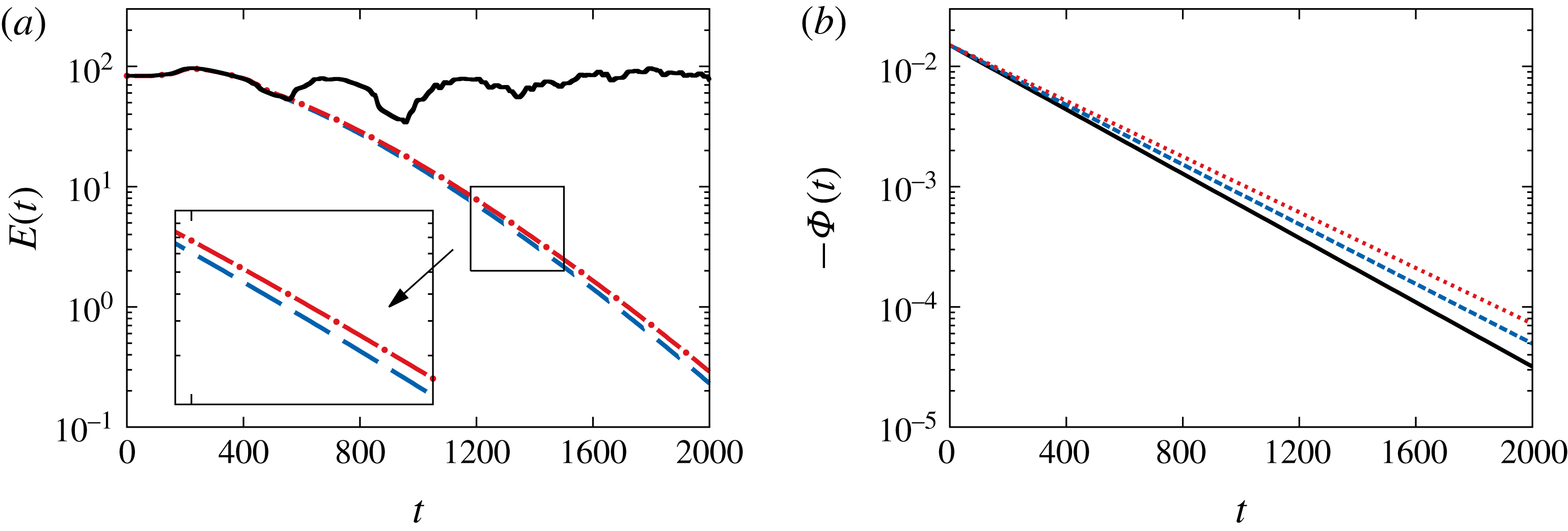
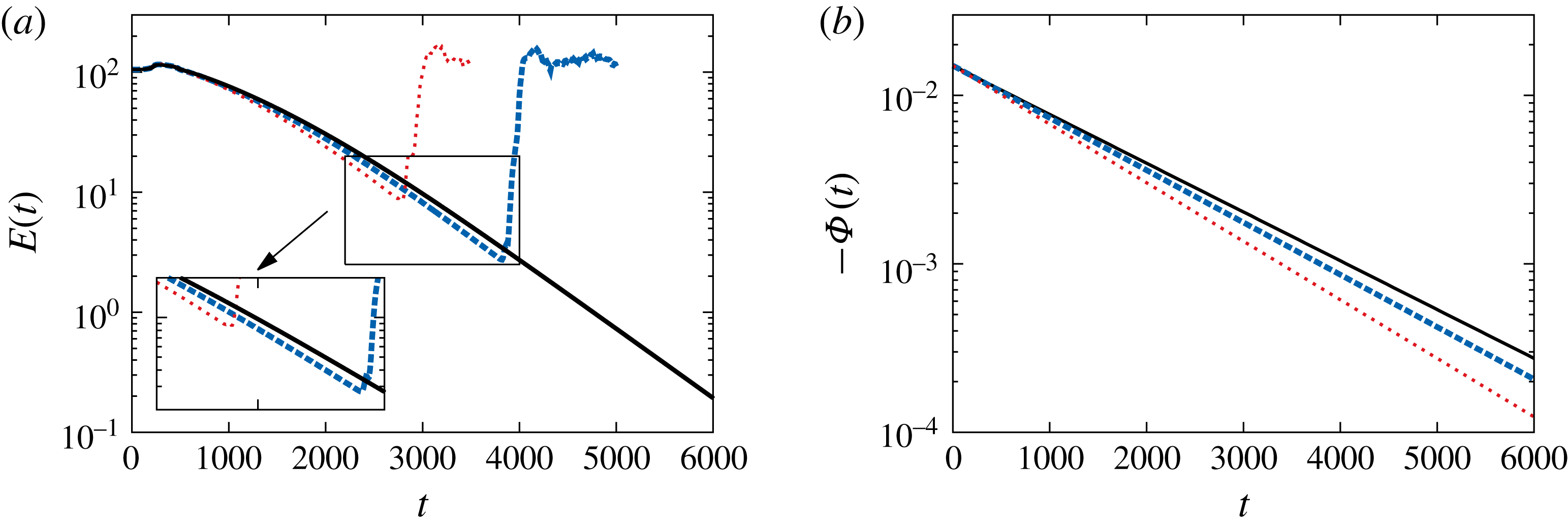
Control of the nonlinear dynamics at
 $Re=610$
. Energy of the perturbation
 $E(t)=\int _{\unicode[STIX]{x1D6FA}}\boldsymbol{u}^{2}\text{d}\unicode[STIX]{x1D6FA}/2$
for the controlled dynamics at
 $\unicode[STIX]{x1D6FE}=1.06\times 10^{5}$
(——),
 $\unicode[STIX]{x1D6FE}=1.22\times 10^{5}$
(- - - -),
 $\unicode[STIX]{x1D6FE}=1.41\times 10^{5}$
(– ⋅ – ⋅ –) using
 ${\mathcal{J}}_{1}$
(a). Associated control laws (b) with
 $\unicode[STIX]{x1D6F7}_{0}=-1.5\times 10^{-2}$
and where the decay rate
 $\unicode[STIX]{x1D70E}+{\mathcal{G}}K=$
 $-3.10\times 10^{-3}$
(——),
 $-2.86\times 10^{-3}$
(- - - -) and
 $-2.67\times 10^{-3}$
(
 $\cdots \cdots$
).

The control law (5.6) has been used as an open-loop strategy for different values of
 $\unicode[STIX]{x1D6FE}$
in figure 6(a,b) at
 $Re=610$
. This flow configuration is characterized by weakly unstable global modes (Ehrenstein & Gallaire Reference Ehrenstein and Gallaire2008). When subject to a continuous suction forcing
 $\unicode[STIX]{x1D6F7}_{0}=-1.5\times 10^{-2}$
, the area of the recirculation region at steady state
 $A_{rec}=230.4$
decreases and the flow becomes globally stable (Boujo et al.
Reference Boujo, Ehrenstein and Gallaire2013). At this Reynolds number, the decay rate associated with the base flow modification is
 $\unicode[STIX]{x1D70E}\approx -0.02$
. The sensitivity prior to a suction actuator located at the summit of the bump (i.e.
 $x=25$
) is
 ${\mathcal{G}}=1.078\times 10^{4}$
. The control strategy (5.6) is integrated in time for different values of the control cost
 $\unicode[STIX]{x1D6FE}$
. Note that increasing
 $\unicode[STIX]{x1D6FE}$
attenuates the decay rate
 $\unicode[STIX]{x1D70E}+{\mathcal{G}}K$
of the controlled base flow modification dynamics. The temporal evolution of the energy for different values of the control cost is shown in figure 6(a). The energy first increases when the suction starts to decrease. This is due to a single vortex, shed from the recirculation region which is rapidly advected downstream. When the control decrease is sufficiently slow, the decay of the energy decreases nearly exponentially in time, according to the control decay rate imposed by the actuator and shown in figure 6(b). However, for
 $\unicode[STIX]{x1D6FE}<1.05\times 10^{5}$
, that is for lower control costs, the control is not capable of stabilizing the dynamics and after
 $600$
time units the flow returns to a saturated nonlinear state (cf. figure 6
a).
The control of the fully nonlinear flow state is now considered using the suction control strategy described in § 5.1 at
 $Re=650$
. The recirculation area of the steady state is
 $A_{rec}=246$
and the sensitivity analysis provides the value
 ${\mathcal{G}}=1.49\times 10^{4}$
, the decay rate being
 $\unicode[STIX]{x1D70E}\approx -0.003$
. The initial suction control
 $\unicode[STIX]{x1D6F7}_{0}=-1.5\times 10^{-2}$
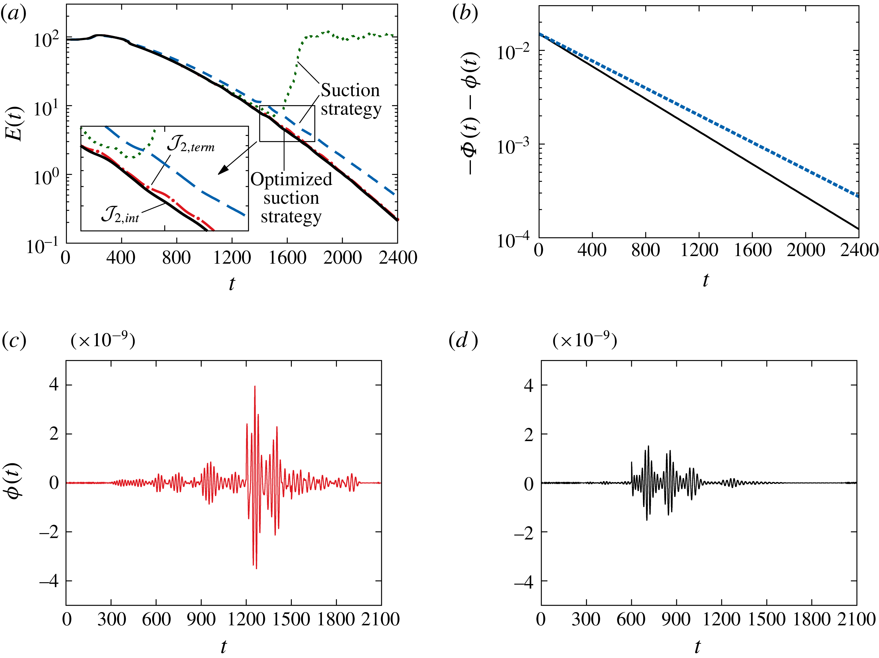
proved suitable for reaching a steady state. The time evolution of the energy shown in figure 7(a) produces similar dynamics to what was previously observed in the
 $Re=610$
case. As shown in figure 7(a), a value of
 $\unicode[STIX]{x1D6FE}=3.6\times 10^{5}$
and thus a time-dependent decreasing suction of the form (5.6) with
 $\unicode[STIX]{x1D70E}+{\mathcal{G}}K=-3.3\times 10^{-3}$
forces the flow to return to a steady state. Decreasing
 $\unicode[STIX]{x1D6FE}$
to
 $\unicode[STIX]{x1D6FE}=2.5\times 10^{5}$
and thus
 $\unicode[STIX]{x1D70E}+{\mathcal{G}}K=-2\times 10^{-3}$
(cf. figure 7
b) appears to offer a faster control. However, at
 $t\approx 1500$
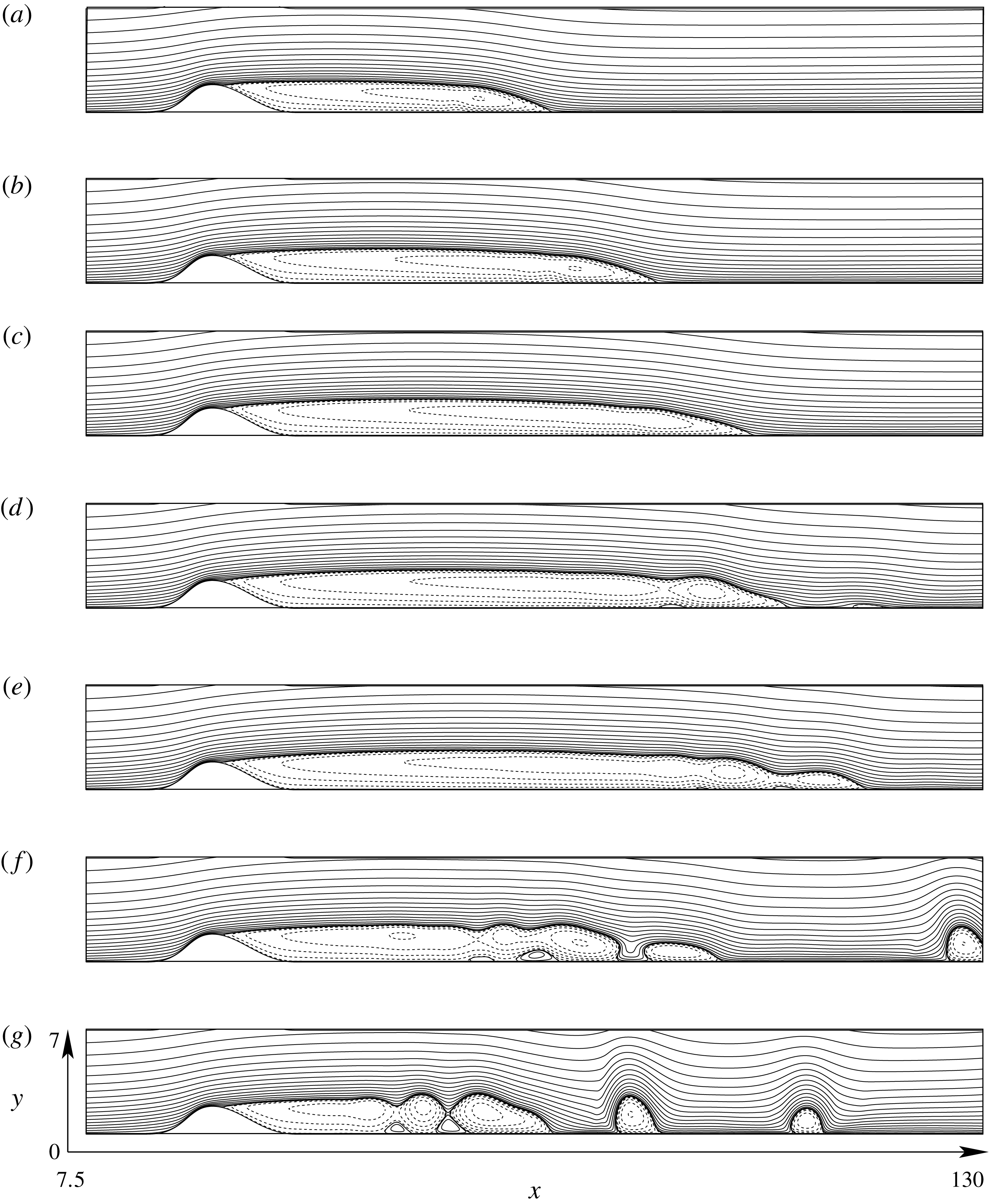
, transient growth followed by a (low-frequency) instability makes the flow to return to the saturated nonlinear regime (see figure 8 for a sequence illustrating this process). This failing strategy is characterized by a large amount of transient growth at
 $t\approx 1500$
and was studied for similar flow conditions by Ehrenstein & Gallaire (Reference Ehrenstein and Gallaire2008).
Control of the nonlinear dynamics at
 $Re=650$
. Energy of the perturbation for the open-loop control strategy at
 $\unicode[STIX]{x1D6FE}=2.5\times 10^{5}$
(
 $\cdots \cdots$
), with additional optimized dynamics using
 ${\mathcal{J}}_{2,term}$
(– ⋅ – ⋅ –) and using
 ${\mathcal{J}}_{2,int}$
(——); open-loop control for
 $\unicode[STIX]{x1D6FE}=3.6\times 10^{5}$
(- - - -) (a). Optimal control laws
 $\unicode[STIX]{x1D6F7}(t)+\unicode[STIX]{x1D719}(t)$
computed with
 ${\mathcal{J}}_{2,term}$
(b) at
 $\unicode[STIX]{x1D6FE}=2.5\times 10^{5}$
(——) and
 $\unicode[STIX]{x1D6FE}=3.6\times 10^{5}$
(- - - -); for
 $\unicode[STIX]{x1D6FE}=2.5\times 10^{5}$
,
 $\unicode[STIX]{x1D719}(t)$
computed with
 ${\mathcal{J}}_{2,term}$
(c) and
 $\unicode[STIX]{x1D719}(t)$
computed with
 ${\mathcal{J}}_{2,int}$
(d).

To prevent the flow transiting back to the perturbed state (at
 $\unicode[STIX]{x1D6FE}=2.5\times 10^{5}$
), the strategy described in § 5.2 has been applied during the time marching in order to suppress the transients. The control signal
 $\unicode[STIX]{x1D719}(t)$
is solved for the time of optimization
 $[T_{0},T_{1}]$
(with
 $T_{1}-T_{0}=600$
), until convergence of the gradient between two iterates with a residuum
 $10^{-3}$
is achieved. Note that in Passaggia & Ehrenstein (Reference Passaggia and Ehrenstein2013), the convergence of the gradient appeared to be difficult to achieve and the gradient (5.16) had to be evaluated
 $10$
to
 $15$
times for each time window, in order to find a local minimum of their cost function. In the present investigations, only two to three evaluations of (5.16) for each optimization time window proved to be necessary to decrease (5.8) or (5.9) as well as (5.16) by two orders of magnitude and hence to converge to a local minimum of the cost functions. The control is then restarted for a time shifted by half the time of optimization (
 $T_{a}=(T_{1}-T_{0})/2=300$
) and marched for a new time interval
 $[T_{0}+T_{a},T_{1}+T_{a}]$
. Note that Passaggia & Ehrenstein (Reference Passaggia and Ehrenstein2013) considered an objective function based on the energy, whereas here the square of the time derivative of the velocity is considered. Also, the initial state they departed from was a fully developed nonlinear state associated with the vortex shedding showed in figure 1(c). In the present study, the suction state from which we start does not exhibit vortex shedding and proves to be more convenient to control the flow back to a steady state.
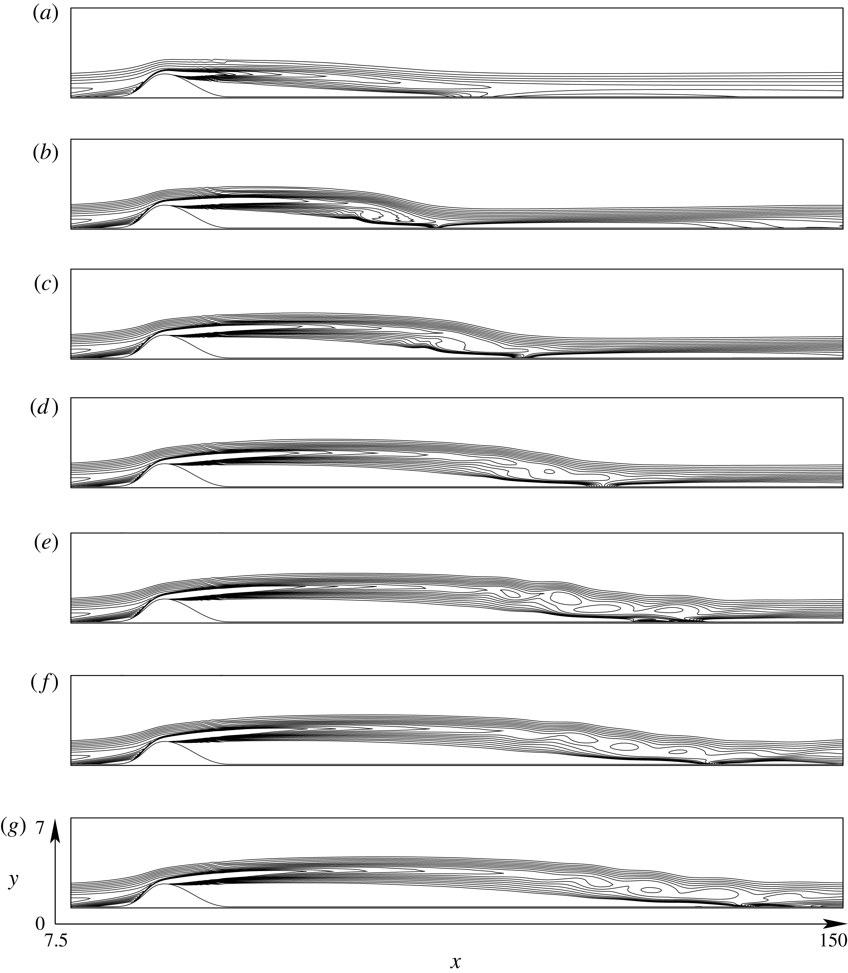
Sequence of streamlines for the failing open-loop strategy for
 $\unicode[STIX]{x1D6FE}=2.5\times 10^{5}$
and
 $Re=650$
at (a)
 $T=300$
, (b)
 $T=600$
, (c)
 $T=900$
, (d)
 $T=1200$
, (e)
 $T=1500$
, (f)
 $T=1800$
and (g)
 $T=2100$
for the terminal time control strategy, using the objective function
 ${\mathcal{J}}_{2,term}$
. Note that the
 $y$
axis is stretched compared to the
 $x$
axis.

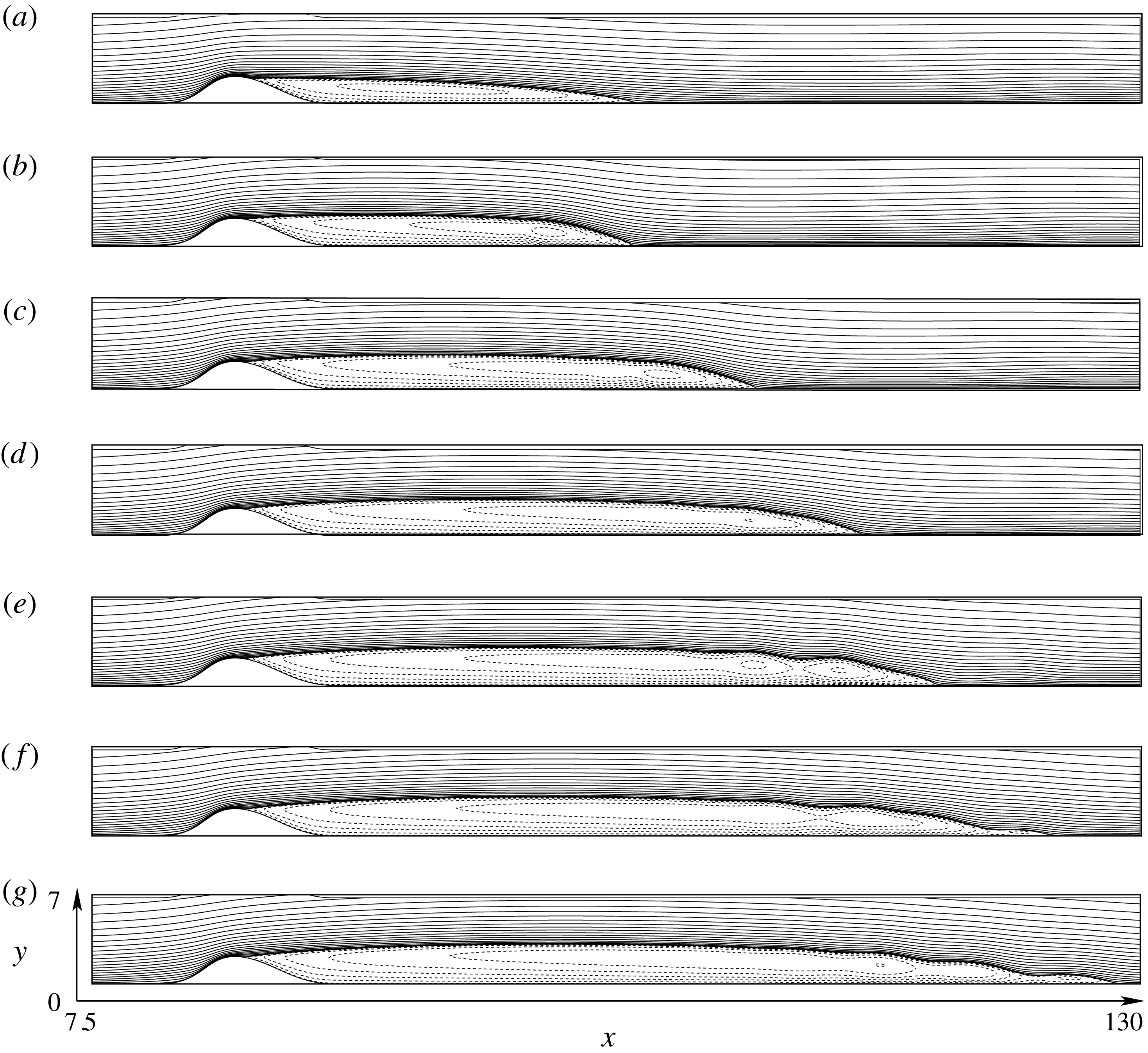
Sequence of streamlines for the adjoint-based controlled strategy for
 $\unicode[STIX]{x1D6FE}=2.5\times 10^{5}$
and
 $Re=650$
at (a)
 $T=0$
, (b)
 $T=300$
, (c)
 $T=600$
, (d)
 $T=900$
, (e)
 $T=1200$
, (f)
 $T=1500$
and (g)
 $T=1800$
for the terminal time control strategy, using the objective function
 ${\mathcal{J}}_{2,term}$
. Note that the
 $y$
axis is stretched compared to the
 $x$
axis.

Same as figure 9 showing the time evolution of arbitrary contours of positive vorticity. Note that the
 $y$
axis is stretched compared to the
 $x$
axis.

Both control objective functions
 ${\mathcal{J}}_{2,term}$
and
 ${\mathcal{J}}_{2,int}$
proved suitable for controlling the low-frequency flapping-type instability (typical for this recirculation bubble as discussed in Ehrenstein & Gallaire (Reference Ehrenstein and Gallaire2008)). A closer look at the evolution of the energy in figure 7(a) shows that
 ${\mathcal{J}}_{2,int}$
performs however a little better than
 ${\mathcal{J}}_{2,term}$
. The control laws for both objective functions
 ${\mathcal{J}}_{2}$
are shown in figure 7(c,d). The integral time control strategy essentially controls the transients early in the simulation, in the time interval
 $[600,1100]$
, whereas the terminal control mainly acts later in time (in the interval
 $[1200,1800]$
). Also note that the terminal time control has a larger maximal amplitude. Both control strategies
 $\unicode[STIX]{x1D719}(t)$
are characterized by two frequencies. Performing a fast Fourier transform of
 $\unicode[STIX]{x1D719}(t)$
, a high frequency
 $f_{high}\approx 4.67\times 10^{-2}$
associated with the unstable global modes and
 $f_{low}\approx 4.76\times 10^{-3}$
corresponding to the low-frequency instability dominate. These different instability characteristics are reported in Ehrenstein & Gallaire (Reference Ehrenstein and Gallaire2008) and Passaggia et al. (Reference Passaggia, Leweke and Ehrenstein2012) for this bump-induced separated boundary-layer flow. Note that the amplitude of the control for the transients
 $\unicode[STIX]{x1D719}(t)$
is
 $5$
to
 $6$
orders of magnitudes smaller than the suction strategy
 $\unicode[STIX]{x1D6F7}(t)$
and is therefore not noticeable in figure 7(b).
The time evolution of the flow computed for the objective function
 ${\mathcal{J}}_{2,term}$
is shown in figure 9. Starting from the modified steady state, subject to the steady suction
 $\unicode[STIX]{x1D6F7}_{0}$
, the recirculation region extends slowly towards its original length. As pointed out earlier, the effect of the low-frequency flapping instability starts to be visible at
 $t=1200$
together with a very weak vortex shedding observed at
 $t=1200$
. At time
 $t=2400$
, the flow is completely stabilized and the flow resembles the steady state, shown in figure 1(a). The effect of the control can be observed in figure 10(e–g) by mean of iso-contours of vorticity. The shear layer is seen to display a train of vortices upstream of the reattachment region. This process is the result of the wave-cancelling phenomena induced by the control (Joslin et al.
Reference Joslin, Gunzburger, Nicolaides, Erlebacher and Hussaini1995). Small amplitude wave packets excited upstream by the actuator are amplified in the shear layer and stabilize the flapping instability. Note that for
 $\unicode[STIX]{x1D6FE}<2.2\times 10^{5}$
the suction control fails at stabilizing the unstable dynamics.
The same procedure is used for a more unstable case at
 $Re=700$
. For this highly supercritical flow regime, the recirculation area of the steady state increases to
 $A_{rec}=266.2$
. The sensitivity analysis provides the value
 ${\mathcal{G}}=1.255\times 10^{4}$
and the initial suction control is again
 $\unicode[STIX]{x1D6F7}_{0}=-1.5\times 10^{-2}$
. Note that in that case the absolute value of the decay rate of the base flow modification decreases to
 $-\unicode[STIX]{x1D70E}=0.00115$
, which is much smaller than the value
 $-\unicode[STIX]{x1D70E}\approx 0.004$
found at
 $Re=650$
. The control law
 $\unicode[STIX]{x1D6F7}(t)$
is expected to behave accordingly and this is observed in figure 11(a). Indeed, the value of
 $\unicode[STIX]{x1D6FE}=2.25\times 10^{6}$
and thus
 $\unicode[STIX]{x1D70E}+{\mathcal{G}}K=-6.67\times 10^{-4}$
(cf. figure 11
b) is seen to be appropriate to control the flow back to a steady state. Attempts to control the transients associated with faster control strategies (i.e.
 $\unicode[STIX]{x1D6FE}=1.56\times 10^{6}$
and
 $\unicode[STIX]{x1D6FE}=1.96\times 10^{6}$
) were made. However at
 $t\approx 2600$
or
 $t\approx 4000$
, the transients followed by the low-frequency flapping instability appear to be uncontrollable using the present optimization algorithm.
The transients associated with this phenomena trigger a wave packet near the separation point which is likely to be uncontrollable using a single actuator (Ehrenstein et al.
Reference Ehrenstein, Passaggia and Gallaire2011; Passaggia & Ehrenstein Reference Passaggia and Ehrenstein2013). This finite amplitude wave packet is sensitive to the decay rate of the control law
 $\unicode[STIX]{x1D6F7}(t)$
(cf. figure 11). Indeed, when controlled too fast, the flow triggers transient growth and the flow returns to the saturated nonlinear regime. As can be seen in figure 11, the more expensive (in terms of suction amplitude) control with
 $\unicode[STIX]{x1D6FE}=2.25\times 10^{6}$
leads however to a continuous decrease of the perturbation energy and no transient dynamics has been observed up to
 $t=8000$
using this suction strategy. We did not attempt to progress further in time, but the base flow modification will ultimately become negligible. As the base flow approaches the steady state, the self-excited instabilities associated with the resonator dynamics (Ehrenstein & Gallaire Reference Ehrenstein and Gallaire2008; Passaggia et al.
Reference Passaggia, Leweke and Ehrenstein2012) are expected to grow again. However, in this quasi-linear regime, Passaggia & Ehrenstein (Reference Passaggia and Ehrenstein2013) already performed the control of the self-excited instabilities successfully by computing
 $\unicode[STIX]{x1D719}(t)$
using the direct–adjoint optimization procedure.
Control of the nonlinear dynamics at
 $Re=700$
. Energy of the perturbation for the suction strategy at
 $\unicode[STIX]{x1D6FE}=2.25\times 10^{6}$
(——),
 $\unicode[STIX]{x1D6FE}=1.96\times 10^{6}$
(- - - -) and
 $\unicode[STIX]{x1D6FE}=1.56.\times 10^{6}$
(
 $\cdots \cdots$
) (a). Associated optimal control laws
 $\unicode[STIX]{x1D6F7}(t)$
(b).

7 Concluding discussion
A new control methodology has been proposed, using sensitivity analysis associated with base flow modification, optimal base flow control and Lagrangian-based optimization procedures for transient perturbation dynamics. As a flow example a separated boundary layer has been considered and it is shown, that when starting the simulation far from the steady state, it is possible to control this globally unstable flow using a time vanishing suction strategy at the wall, at least for sufficiently slow exponential suction decay rates. The present strategy takes advantage of the high sensitivity of the base flow modification to suppress the instabilities and successfully drive the flow back to its steady state. The present approach to control the base flow modification leads to a simple expression for the slowly decaying suction control that could be easily implemented in an experiment. The base flow modification could for instance be inferred from the difference between a local measurement of the flow and numerically computed steady state data. This suction strategy to control the base flow can be further optimized when aiming at a lower control cost, using a Lagrangian-based optimization capable of suppressing transient dynamics.
A recent study showed that the augmented Lagrangian approach could for instance be used to control the flow behind a cylinder (Flinois & Colonius Reference Flinois and Colonius2015) for values of the Reynolds number well beyond criticality. However the method requires very long time horizons for the optimization, which becomes numerically intractable for complex flow dynamics or three-dimensional configurations. The present approach, combining base flow modification control and optimization using the augmented Lagrangian approach, could be a possibility to reduce the time horizons, which is the limiting factor in the case of complex three-dimensional applications for flow optimization algorithms.
The decay rate at which the flow can be controlled appears to be essentially limited by the effects of transient growth. A more robust approach would consist in redesigning the control and assign the long time suction strategy to asymptotically reach a finite value, associated with a more stable steady state. Also, more actuators could be implemented inside the recirculation region or upstream of the bump, which could provide more leverage on the control of the base flow modification.
Finite amplitude perturbations or external noise disturbances would also be a limiting factor, when considering real separated flow cases at high Reynolds numbers. In particular, the control of incoming boundary-layer instabilities upstream of the separation region is likely to be mandatory, in order to decrease or suppress the noise amplified by the boundary layer. Control methods for boundary-layer instabilities in the absence of a pressure gradient have already been proposed and could be implemented (Joslin et al. Reference Joslin, Gunzburger, Nicolaides, Erlebacher and Hussaini1995; Bagheri, Brandt & Henningson Reference Bagheri, Brandt and Henningson2009; Semeraro et al. Reference Semeraro, Pralits, Rowley and Henningson2013).
Our expression for the control of the base flow modification leads to an LQ controller that is equivalent to a proportional controller in the case of a single mode, associated with the decay of the base flow modification. Our approach can be extended to include a larger part of the stable spectrum, for instance including all the modes associated with eigenvalues located along the real axis. In the same perspective, modes with a very small frequency could also be considered included. In addition, the present method could be used in a closed-loop set-up considering only the very slow dynamics, using a Kalman filter and a reduced-order model of the base flow modification. The open-loop strategy of the base flow could be redesigned by solving the differential Riccati equation where the decay rate of the base flow modification
 $\unicode[STIX]{x1D70E}$
could be computed as a function of the initial suction amplitude
 $\unicode[STIX]{x1D6F7}_{0}$
. Methods such as nonlinear control and speed control (Geering Reference Geering2007) where the cost function depends on the amplitude of the base flow modification are also interesting alternatives.
In the scope of extending the present work to the three-dimensional configuration, both upstream disturbances and the effect of increasing Reynolds numbers could be addressed by designing a control strategy that modifies the structure of the recirculation region in the spanwise direction
 $z$
. Indeed, the stabilizing effect of spanwise-varying modifications on both transient and self-excited instabilities is now well established (Cossu & Brandt Reference Cossu and Brandt2002; Bagheri & Hanifi Reference Bagheri and Hanifi2007; Hwang, Kim & Choi Reference Hwang, Kim and Choi2013). Boujo, Fani & Gallaire (Reference Boujo, Fani and Gallaire2015) recently showed that optimal spanwise-varying flow modifications can substantially decrease transient growth in a shear layer. Such alternatives will probably have to be considered for a more robust control strategy when considering a three-dimensional flow geometry.
The present strategy could be tested in an experiment, first imposing a suction at the summit of the bump and second varying the decay rate of the suction. At least in the near critical case, the present slowly decaying suction strategy should improve the stability of the system and delay the transition to turbulence beyond the reattachment region.
Acknowledgements
The project leading to this publication has received funding from Excellence Initiative of Aix-Marseille University – A*MIDEX, a French ‘Investissements d’Avenir’ programme. It has been carried out in the framework of the Labex MEC. We would also like to acknowledge the anonymous referees for their through reviews and constructive suggestions.
Appendix A. Dynamic mode decomposition
In this section we provide the steps used to perform the dynamic mode decomposition in § 4.1. Following the algorithm of Schmid (Reference Schmid2010), snapshots of the velocity
 $\boldsymbol{U}(\boldsymbol{x},t)$
are stored for instance at every
 $\unicode[STIX]{x0394}t=3$
such that
 $$\begin{eqnarray}\unicode[STIX]{x1D647}_{1}^{n}=\left[\boldsymbol{U}(\boldsymbol{x},t+\unicode[STIX]{x0394}t),\boldsymbol{U}(\boldsymbol{x},t+2\unicode[STIX]{x0394}t),\ldots ,\boldsymbol{U}(\boldsymbol{x},t+n\unicode[STIX]{x0394}t)\right],\end{eqnarray}$$
where
 $n=600$
is the number of snapshots stored in the observations matrix
 $\unicode[STIX]{x1D647}_{1}^{n}$
. Here the subscript is the number of the first snapshot stored in the observation matrix and the superscript is the number of the last snapshot stored in the sequence. To extract the dominant features of the sequence (A 1), the
 $n\text{th}$
vector is expressed as a function of the previous realizations, namely
 $$\begin{eqnarray}\boldsymbol{U}(\boldsymbol{x},t+n\unicode[STIX]{x0394}t)=a_{1}\boldsymbol{U}(\boldsymbol{x},t+\unicode[STIX]{x0394}t)+a_{2}\boldsymbol{U}(\boldsymbol{x},t+2\unicode[STIX]{x0394}t)+\cdots +a_{n-1}\boldsymbol{U}(\boldsymbol{x},t+(n-1)\unicode[STIX]{x0394}t)+\boldsymbol{r},\end{eqnarray}$$
where
 $\boldsymbol{r}$
is the residual vector, which in matrix form reads
 $$\begin{eqnarray}\boldsymbol{U}(\boldsymbol{x},t+n\unicode[STIX]{x0394}t)=\unicode[STIX]{x1D647}_{1}^{n-1}\boldsymbol{a}+\boldsymbol{r},\end{eqnarray}$$
where
 $\boldsymbol{a}^{\text{T}}=[a_{1},a_{2},\ldots ,a_{n-1}]$
. As shown by (Ruhe Reference Ruhe1984), the transition matrix
 $\unicode[STIX]{x1D64E}$
, defined by
 $$\begin{eqnarray}\unicode[STIX]{x1D647}_{2}^{n}=\unicode[STIX]{x1D647}_{1}^{n-1}\unicode[STIX]{x1D64E}+\boldsymbol{r}\boldsymbol{e}_{n-1}^{\text{T}},\end{eqnarray}$$
is of companion type and
 $\boldsymbol{e}_{n-1}^{\text{T}}$
is the
 $(n-1)\text{th}$
unit vector. The only unknowns are the coefficients
 $\boldsymbol{a}$
, stored in the last column of
 $\unicode[STIX]{x1D64E}$
. Rather than computing the
 $a$
coefficients using for instance, a least squares procedure (Rowley et al.
Reference Rowley, Mezić, Bagheri, Schlatter and Henningson2009), which can lead to an ill-conditioned companion matrix
 $\unicode[STIX]{x1D64E}$
(Schmid Reference Schmid2010), it is of advantage to regularize the matrix
 $\unicode[STIX]{x1D64E}$
using a proper orthogonal decomposition (POD), by performing a singular value decomposition (SVD) of
 $\unicode[STIX]{x1D647}_{1}^{n-1}$
(Schmid Reference Schmid2010) such that
 $$\begin{eqnarray}\unicode[STIX]{x1D647}_{1}^{n-1}=\boldsymbol{V}\unicode[STIX]{x1D6F4}\boldsymbol{W}^{H},\quad \text{ resulting in }\tilde{\unicode[STIX]{x1D64E}}=\boldsymbol{V}^{H}\unicode[STIX]{x1D647}_{2}^{n}\boldsymbol{W}\unicode[STIX]{x1D6F4}^{-1},\end{eqnarray}$$
where the superscript
 $^{H}$
denotes the conjugate transpose. Note that only the non-zero singular vectors
 $\boldsymbol{v}$
,
 $\boldsymbol{w}$
, associated with singular values
 $\unicode[STIX]{x1D700}\geqslant 10^{-8}$
are retained in (A 5), for the projection onto the POD modes
 $\boldsymbol{V}$
.
The modal structures of the DMD modes
 $\unicode[STIX]{x1D711}$
are extracted from the matrix
 $\tilde{\unicode[STIX]{x1D64E}}$
such that
 $$\begin{eqnarray}\unicode[STIX]{x1D711}_{k}=\boldsymbol{V}\boldsymbol{y}_{k},\end{eqnarray}$$
with
 $\boldsymbol{y}_{k}$
, the
 $k\text{th}$
eigenvector of
 $\tilde{\unicode[STIX]{x1D64E}}$
such that
 $\tilde{\unicode[STIX]{x1D64E}}\boldsymbol{y}_{k}=\unicode[STIX]{x1D707}_{i}\boldsymbol{y}_{k}$
and
 $\boldsymbol{V}$
are the left singular vectors computed in (A 5). The continuous time eigenvalues
 $\unicode[STIX]{x1D70E}_{k}$
are computed using the transformation
 $$\begin{eqnarray}\unicode[STIX]{x1D70E}_{k}=\log (\unicode[STIX]{x1D707}_{k})/\unicode[STIX]{x0394}t,\end{eqnarray}$$
where the
 $\log$
is the complex logarithm.
Appendix B. Linear quadratic controller
In this section, we provide the main steps to derive the Riccati equation (5.5). Following the model described in § 5.1 for the base flow modification dynamics subject to a time-dependent suction, one gets the first-order system
 $$\begin{eqnarray}\displaystyle \frac{\text{d}\,\unicode[STIX]{x1D6FF}A_{rec}(t)}{\text{d}t} & = & \displaystyle \unicode[STIX]{x1D70E}\unicode[STIX]{x1D6FF}A_{rec}(t)+{\mathcal{G}}\unicode[STIX]{x1D6F7}(t),\end{eqnarray}$$
 $$\begin{eqnarray}\displaystyle \unicode[STIX]{x1D6F7}(t) & = & \displaystyle K\unicode[STIX]{x1D6FF}A_{rec}(t).\end{eqnarray}$$
 $\unicode[STIX]{x1D6F7}(t):[0,\infty )$
, such that the controllable system (B 1a,b
) is transferred from an initial state
 $\unicode[STIX]{x1D6FF}A_{rec}(t=0)$
, to an arbitrary final state
 $\unicode[STIX]{x1D6FF}A_{rec}(t\rightarrow \infty )=0$
such that the cost functional (5.3) is maximized and attains a finite optimal value. The time evolution of the control system (B 1a,b
) and the cost function (5.3) are ruled by the Hamiltonian
 $$\begin{eqnarray}{\mathcal{H}}=\unicode[STIX]{x1D6FF}A_{rec}^{2}(t)+\unicode[STIX]{x1D6FE}\unicode[STIX]{x1D6F7}^{2}(t)+Z({\mathcal{G}}\unicode[STIX]{x1D6F7}(t)+\unicode[STIX]{x1D70E}\unicode[STIX]{x1D6FF}A_{rec}(t)),\end{eqnarray}$$
where a co-state variable
 $Z(t)$
has been introduced. Taking derivatives prior to the state, the co-state and the control yields the necessary conditions for optimality (see Geering Reference Geering2007, pp. 41–42) such that
 $$\begin{eqnarray}\displaystyle \unicode[STIX]{x1D735}_{Z}{\mathcal{H}} & = & \displaystyle \frac{\text{d}\unicode[STIX]{x1D6FF}A_{rec}}{\text{d}t}=\unicode[STIX]{x1D70E}\unicode[STIX]{x1D6FF}A_{rec}+{\mathcal{G}}\unicode[STIX]{x1D6F7},\end{eqnarray}$$
 $$\begin{eqnarray}\displaystyle \unicode[STIX]{x1D735}_{\unicode[STIX]{x1D6FF}A_{rec}}{\mathcal{H}} & = & \displaystyle \frac{\text{d}Z}{\text{d}t}=\unicode[STIX]{x1D70E}Z+\unicode[STIX]{x1D6FF}A_{rec},\end{eqnarray}$$
 $$\begin{eqnarray}\displaystyle \unicode[STIX]{x1D735}_{\unicode[STIX]{x1D6F7}}{\mathcal{H}} & = & \displaystyle \unicode[STIX]{x1D6FE}\unicode[STIX]{x1D6F7}+Z{\mathcal{G}},\end{eqnarray}$$
 $$\begin{eqnarray}\displaystyle \unicode[STIX]{x1D6FF}A_{rec}(t_{0}) & = & \displaystyle {\mathcal{G}}\unicode[STIX]{x1D6F7}_{0}.\end{eqnarray}$$
 $$\begin{eqnarray}\unicode[STIX]{x1D6F7}=-\unicode[STIX]{x1D6FE}^{-1}{\mathcal{G}}Z.\end{eqnarray}$$
Substituting this control in the evolution equations (B 3c ) results in a two-point initial value problem
 $$\begin{eqnarray}\displaystyle \frac{\text{d}\unicode[STIX]{x1D6FF}A_{rec}}{\text{d}t} & = & \displaystyle \unicode[STIX]{x1D70E}\unicode[STIX]{x1D6FF}A_{rec}+{\mathcal{G}}\unicode[STIX]{x1D6F7},\end{eqnarray}$$
 $$\begin{eqnarray}\displaystyle \frac{\text{d}Z}{\text{d}t} & = & \displaystyle \unicode[STIX]{x1D70E}Z+\unicode[STIX]{x1D6FF}A_{rec},\end{eqnarray}$$
 $$\begin{eqnarray}\displaystyle \unicode[STIX]{x1D6F7} & = & \displaystyle -\unicode[STIX]{x1D6FE}^{-1}{\mathcal{G}}Z,\end{eqnarray}$$
 $$\begin{eqnarray}\displaystyle \unicode[STIX]{x1D6FF}A_{rec}(t_{0}) & = & \displaystyle {\mathcal{G}}\unicode[STIX]{x1D6F7}_{0},\end{eqnarray}$$
 $$\begin{eqnarray}\displaystyle Z(t_{1}) & = & \displaystyle \unicode[STIX]{x1D6FF}A_{rec}(t_{1}).\end{eqnarray}$$
 $$\begin{eqnarray}Z(t)=X(t)\unicode[STIX]{x1D6FF}A_{rec}(t),\end{eqnarray}$$
differentiating (B 6) with respect to time and making use of equations (B 5a–c ) reduces to a single equation
 $$\begin{eqnarray}\unicode[STIX]{x1D6FF}A_{rec}\frac{\text{d}X}{\text{d}t}+X\frac{\text{d}\unicode[STIX]{x1D6FF}A_{rec}}{\text{d}t}=\unicode[STIX]{x1D6FF}A_{rec}\frac{\text{d}X}{\text{d}t}+X(\unicode[STIX]{x1D70E}-\unicode[STIX]{x1D6FE}^{-1}{\mathcal{G}}^{2}X)\unicode[STIX]{x1D6FF}A_{rec}=-\unicode[STIX]{x1D6FF}A_{rec}-\unicode[STIX]{x1D70E}X\unicode[STIX]{x1D6FF}A_{rec},\end{eqnarray}$$
which is the differential Riccati equation
 $$\begin{eqnarray}\left(-\frac{\text{d}X}{\text{d}t}-\unicode[STIX]{x1D6FE}^{-1}X^{2}{\mathcal{G}}^{2}+2\unicode[STIX]{x1D70E}X+1\right)\unicode[STIX]{x1D6FF}A_{rec}\equiv 0.\end{eqnarray}$$
Because (5.1) has constant coefficients, the time dependence can be dropped and (B 8) reduces to the algebraic Riccati equation (5.5).